1. Introduction
Italian building code (D.M. 17.01.2018) [
1] as well as several national codes prescribe seismic response analyses for specific site conditions. These analyses, typically using 1D codes, model the vertical propagation of shear waves through a soil column. The approach is either linear or equivalent nonlinear, though these methods are unable to directly assess the seismic site instability. In practice, even in high-risk areas, simplified procedures are used instead.
While research has developed rigorous, highly sophisticated soil constitutive models to address these issues, their use in practical design is limited due to the complexity of calibrating numerous parameters. Methods balancing scientific rigor with practical application were developed for specific earthwork types (e.g.,[
2]), but a lack of general solutions persists. This may stem from a historical view that soil failure under dynamic conditions is a rare event, only occurring during high-intensity earthquakes. However, recent earthquakes (e.g., 2009 L'Aquila, 2012 Emilia, 2016 Central Italy) have challenged this belief, as more timely and accurate damage reconnaissance has allowed engineers and researchers to recognize the manifestations of site instability.
Seismic site instability is essentially due to an increase in shear stresses as a result of wave propagation in deformable soils (collapse and landslides), or decreased effective stresses caused by increasing pore water pressures (subsidence, liquefaction and landslides), resulting in a drastic decrease in soil stiffness and shear strength.
Rigorous numerical modeling of seismic instability requires sophisticated computer codes with advanced constitutive models that incorporate plasticity and volumetric-distortional coupling. These models can simulate localized or generalized failure, but their practical use is challenging due to the difficulty of calibrating numerous parameters reliably.
A compromise between scientific rigor and practical application is achieved through simplified models. Many of these methods are decoupled, meaning they separate the seismic wave propagation problem (solved under free-field conditions) from the estimation of response parameters (e.g., displacement or Cyclic Stress Ratio) using empirical or semi-empirical procedures. While useful for initial screening, these decoupled methods may not adequately capture the highly nonlinear behavior of soils nearing failure.
To address this issue, "coupled" procedures have been developed. Although these methods are effectively decoupled, they are applied at each time step. This approach enables the updating of the soil's strength and damping parameters following each calculation, rendering them suitable for time-domain dynamic response calculations.
For failure problems, several "coupled" stick-slip formulations have been proposed to calculate plastic displacements. SCOSSA (Seismic COde for Stick–Slip Analysis), was developed by Tropeano et al. [
3]. It includes an algorithm to automatically detect critical sliding surfaces, an updated hysteretic constitutive relationship, and a stable iterative solution for kinematic variables.
For liquefaction problems, several studies pointed out the importance of performing effective stress analysis [
4,
5,
6].
SCOSSA-PWP [
7] incorporates a simplified stress-based pore water pressure model [
8] along with one-dimensional consolidation theory [
9]. This model was chosen for its simplicity, consistency with established liquefaction frameworks, ease of implementation, and straightforward parameter quantification. Originally calibrated with laboratory tests, the model was later extended to use common in-situ test data (CPT and SPT)[
10], and more recently DMT [
11].
The code's effectiveness in predicting pore water pressure build-up and dissipation has been validated against physical models in seismic centrifuges [
7,
12,
13] and instrumented field sites [
7,
10,
12]. Comparisons with more complex codes on real and ideal cases [
14,
15] show that SCOSSA provides a slightly more conservative, yet reliable, prediction. Post-analysis results have also been successfully used to predict horizontal displacements [
16] and post-consolidation settlements [
12,
17] in real-world case studies, yielding estimates consistent with observed damage.
This review traces the main steps of the code development, the main features and applications by summarizing the work on the code performed in the last ten years.
2. Main Steps in the Development of the SCOSSA Code
The code was originally developed for evaluating permanent seismic displacements of slopes [
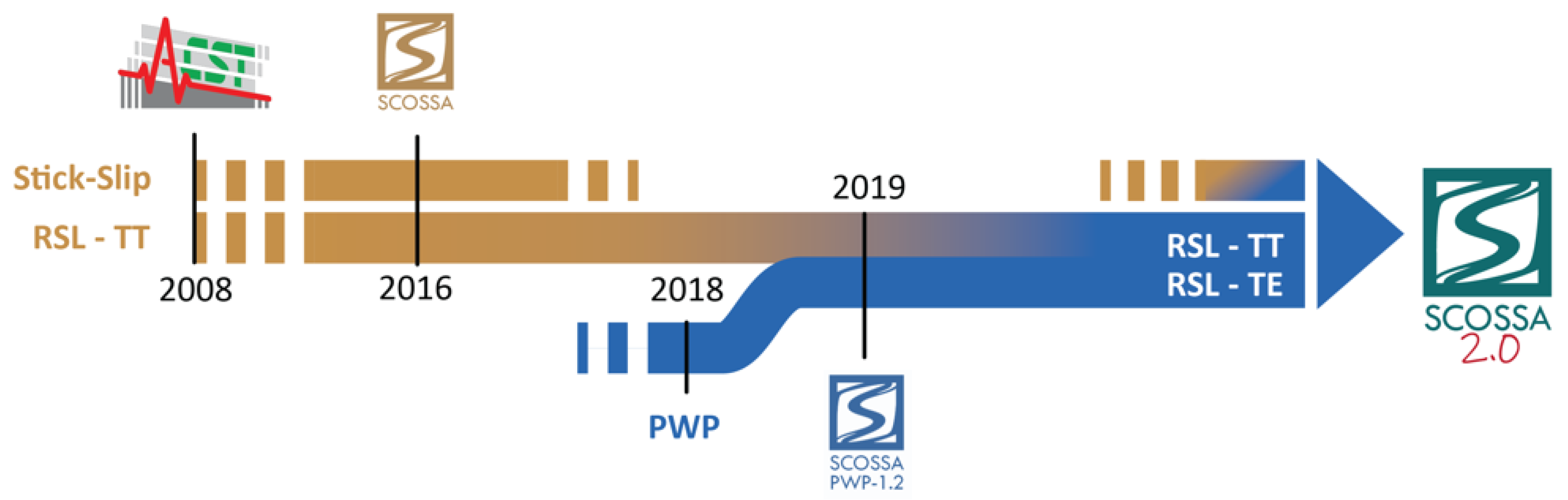
18], considering a stick-slip model (see
Figure 1). In detail, a lumped-mass formulation has been adopted with more generalized assumptions, and the model was implemented in the first version of the computer code, named “ACST” which used an equivalent-linear formulation expressed in the time domain. In Tropeano et al. [
19], the version in non-linear conditions is presented for the first time.
Tropeano et al. [
20] describes a new version, renamed “SCOSSA” (Seismic COde for Stick–Slip Analysis), where (1) the solution of the dynamic equilibrium equations includes the possibility of search for the critical sliding surface automatically, (2) the constitutive relationship models the hysteretic soil behavior, and (3) a stable iterative algorithm solves the system in terms of kinematic variables.
So, initially the code was designed for dynamic analyses in total stress to simulate both the transient response (stick mode) and response in case of formation of a rupture and a sliding surface (stick-slip mode). Two distinct analysis modes were implemented in the code: the 'RSL-TT' module, which solves the equations of motion to provide the site's seismic response under total stress conditions; and the 'Stick-Slip' module, which includes the possibility of a sliding mechanism in the local seismic response. The "RSL-TT" module is used to perform the nonlinear analysis of a soil column composed of horizontal layers under total stress conditions. The "Stick-Slip" module is used to determine the depth of the sliding surface of an indefinite slope and therefore, calculate the sliding response and cumulative displacements.
The ‘RSL-TT’ module for transient seismic response has been verified and validated with other codes during PREdiction of NOn-LINear soil behaviour (PreNoLin) project an international numerical benchmark [
21,
22].
The use ‘Stick-Slip’ modules has been limited to theoretical exercises and few well-documented case histories of slope instability [
20]. Further applications include the modelling of the combined response of soil and building, based on the case study of a structure damaged after the 2009 L’Aquila earthquake [
23].
In the framework of the Chiaradonna PhD thesis, a pore water pressure model following a simplified stress-based approach has been developed [
8] and then implemented in the ‘RSL-TT’ module of the code [
7,
24]. The pore pressure model was implemented using a loosely coupled approach to account for the degradation of soil stiffness and strength. This degradation is a result of the progressive build-up of pore water pressure caused by cyclic shear loading. The new version of the code, hereafter called ‘SCOSSA PWP’, consists of the modified ‘RSL-TT’ module integrated with the above-mentioned pore pressure model and 1D consolidation theory [
9]. The dissipation and redistribution of excess pore water pressure can be activated or deactivated in the analysis settings by allowing the execution of effective stress analysis both in totally undrained or partially drained conditions, respectively.
In the following three main chapters, the calculations performed for solving seismic response analysis in total stress (‘RSL-TT’ module), slope stability (‘Stick-Slip’ module), and liquefaction problems (‘SCOSSA PWP’), are detailed, as well as the available validations.
3. Seismic Response Analysis in Total Stress
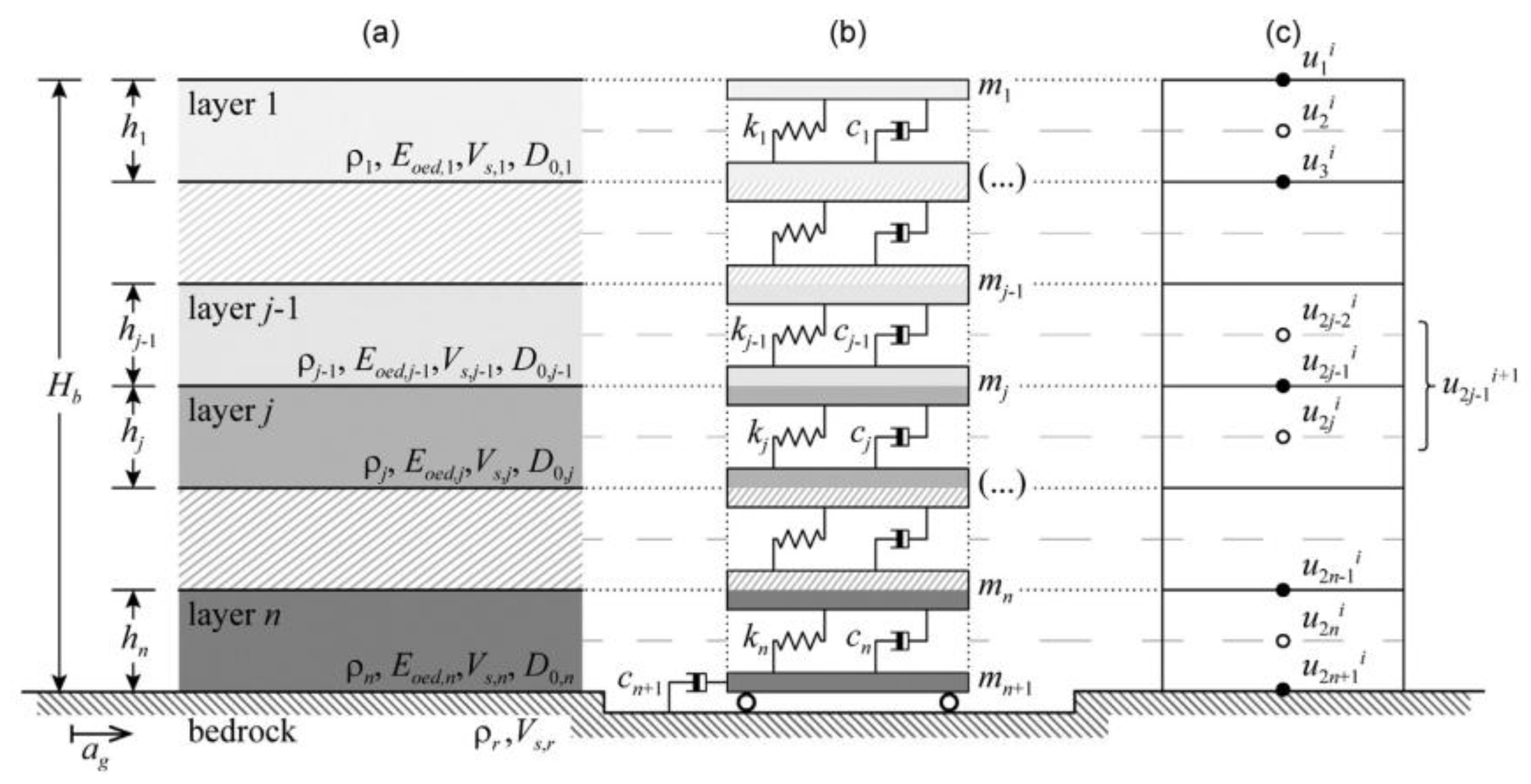
The soil profile is modelled in the code as a system of consistent lumped masses connected by viscous dampers and hysteretic non-linear springs (
Figure 2a, b).
The discretization of the subsurface profile into a lumped parameter system has been automatically implemented within the code. This implementation is based on the Kuhlemeyer and Lysmer [
25] criterion, which mandates that the maximum sub-layer thickness be constrained to a specific fraction (typically 1/6 to 1/8) of the minimum wavelength, which must be accurately transmitted. This maximum thickness is, however, still subjected to a lower bound constraint, which corresponds to the minimum significant thickness (approximately 25 cm).
The code executes non-linear seismic response analyses by solving the dynamic equilibrium of a multiple-degree-of-freedom (MDOF) system in the time domain. The seismic response quantified by absolute displacements,
s, resulting from a base ground motion,
ag (
Figure 2a,b), can be determined through the integration of the following system:
where
f(
t) is the vector of applied forces and
M,
C and
K are the mass, damping and stiffness matrices, respectively. The
f vector can be set as equal to:
where:
- -
i is a vector with each element equal to zero, except for the n-th (for inside motion), or (n + 1)th (for outcrop motion), equal to unity;
- -
vg(t) and sg(t) are, respectively, the velocity and the displacement time histories obtained by numerical integration of input acceleration, ag(t);
- -
cn and kn are, respectively, the viscous damping coefficient and the spring elastic stiffness for the n-th element,
- -
cn+1 = ρrVS,r is the bedrock seismic impedance.
The
M and
K matrices are defined, respectively, from the mass,
mj, and the current spring stiffness,
kj, of a generic soil layer
j, as follows:
where, for the
j-th layer,
ρj,
hj, and
Gj are, respectively, the density, thickness and tangent shear modulus.
The viscous damping matrix,
C, is defined following the full Rayleigh damping formulation [
26]:
where the constants
αR and
βR are set as functions of the minimum soil damping ratio,
ξmin, the fundamental frequency of the subsoil profile and the predominant frequency of the input motion [
27].
An initial updating of the vector of input forces, f(t), is carried out for the i-th time step.
The code numerically integrates the equations by using the Newmark β method [
28]:
γN = 0.5 and βN = 0.25 are the default coefficients, so that the method is unconditionally stable and no numerical damping is introduced.
For a dynamic system with
n degrees of freedom, the system (6) can be easily solved if expressed in the form:
where
x is the vector of the unknown variables:
In Eq. (7),
q is the external forces vector, where the first
n elements are equal to
f, as defined in eq. (2), and the remaining 2
n elements are null;
A and
B are the matrices of the integration method, defined as follows:
where
1 and
0 are the unit and null matrix, respectively, with
n ×
n dimension.
The numerical solution of system (7) is carried out adopting an exact inversion method based on the Crout-Doolittle factorization algorithm, modified for band matrices. The computation of the kinematic variables, i.e., acceleration, velocity and displacement, are obtained from the numerical solution. Then, the shear strain increment, Δγ
j, is computed as:
where Δ
sj = (
sj)
i+1 – (
sj)
i is the displacement variation in the time interval Δ
t, while
hj is the sub-layer thickness.
Given that the stiffness matrix, K, exhibits strain-dependent variability, the initial computational effort involves assuming the stiffness matrix to be equivalent to the value calculated during the preceding time increment.
A continuous stress-strain function is employed to calculate the shear stress increment, Δτj, in the time interval Δt. This calculation is executed as a function of the shear strain level mobilized at the prior time step (via the cyclic response model detailed in section § 3.1).
The current value of stiffness for the
j-th sub-layer,
kj, is calculated by the tangent shear modulus,
Gj, as:
As a consequence, it is possible to define the stiffness matrix from the current shear strain level through equation (11).
An iterative computation needs to be applied at each time step due to the mutual dependency between
K and the solution of the system. In detail, as a first attempt, the stiffness matrix is set equal to the one calculated at the previous time instant, i.e., [
Kt+ 1]
k = 0 =
Kt. The system is solved and the strain, [γ
t+ 1]
k = 0, and stress, [τ
t+ 1]
k = 0, vectors are calculated. Then, the stiffness matrix of the layering is again evaluated as [
Kt + 1]
k = 1. The procedure is iterated until the maximum value of the relative error, ε
rel, of two subsequent solutions, [
xt+ 1]
k - 1 and [
xt + 1]
k, is less than a fixed tolerance value, ε
toll. The maximum value of the relative error, ε
rel is defined as:
3.1. Cyclic Response Model
The non-linear hysteretic behavior of the soil is simulated utilizing an extended formulation of the Modified Kondner-Zelasko (MKZ) hyperbolic model (e.g., [
29]). This model is delineated by two distinct constitutive relationships: one for the initial loading phase and another governing unloading-reloading cycles.
The stress-strain constitutive function (i.e., the backbone curve) for the loading condition is expressed as follows:
where β and
s are two dimensionless factors, γ is the shear strain level,
G0 is the initial shear modulus, γ
r is the reference shear strain.
The stress-strain relationship for unloading-reloading condition can be either defined by the generalized Masing criteria or by considering damping control given by the unload-reload curves proposed by Phillips and Hashash [
30]:
In Eq. (14), γ
c and τ
c are, the reversal shear strain and shear stress, respectively, γ
m is the maximum shear strain reached during the time history, and
F(γ
m) is a damping reduction factor, defined as:
In Eq. (15),
p1,
p2 and
p3 are dimensionless coefficients derived from the optimal fitting of the ratio between the strain-dependent hysteretic damping as measured in laboratory tests, ξ
exp(γ), and the correspondent one calculated via the Masing rules, ξ
Mas(γ);
G(γ
m) represents the secant shear modulus corresponding to the maximum shear strain γ
m (see [
30] for details).
The revised formulation adjusts the Masing unloading-reloading criteria, thereby achieving enhanced correlation with the experimental damping-strain curves, particularly at elevated shear strain levels. In terms of numerical execution, the application of the factor F(γm) concurrently induces a marked progressive reduction in the small-strain shear stiffness, G0, thus simulating a cyclic soil degradation.
Within the SCOSSA framework, the three parameters defining the modified MKZ model (Equation (13)) and the parameters governing the modified Masing rules (Equation (14)) are archived in a database that incorporates established literature relationships [
30]. These relationships are presented to the user during the subsoil data input process via an interface dialog box. Alternatively, these parameters can be calculated specifically for a project through nonlinear multi-regression analysis of the experimental data points for
G(γ)/
G0 and ξ(γ), and subsequently appended to the database. A dedicated utility was integrated into SCOSSA for the interpolation of objective functions. This procedure is executed by an adaptive algorithm that computes the relative minimum value of the multivariate functions, having been enhanced with an optimization protocol to determine the bracketing interval.
3.2. Code Performances at Low-Medium Strains
Soil nonlinearity is a function of the shear strain level mobilized during seismic shaking [
31,
32]. With the aim of showing the performance of the code in both low and medium-high strain levels, two subsections are reported in the following. The first one is related to simulating the behavior of ideal soil columns, the second one is related to a real case study investigated in the framework of the PreNoLin project [
22].
3.2.1. Verification on Ideal Soil Profiles
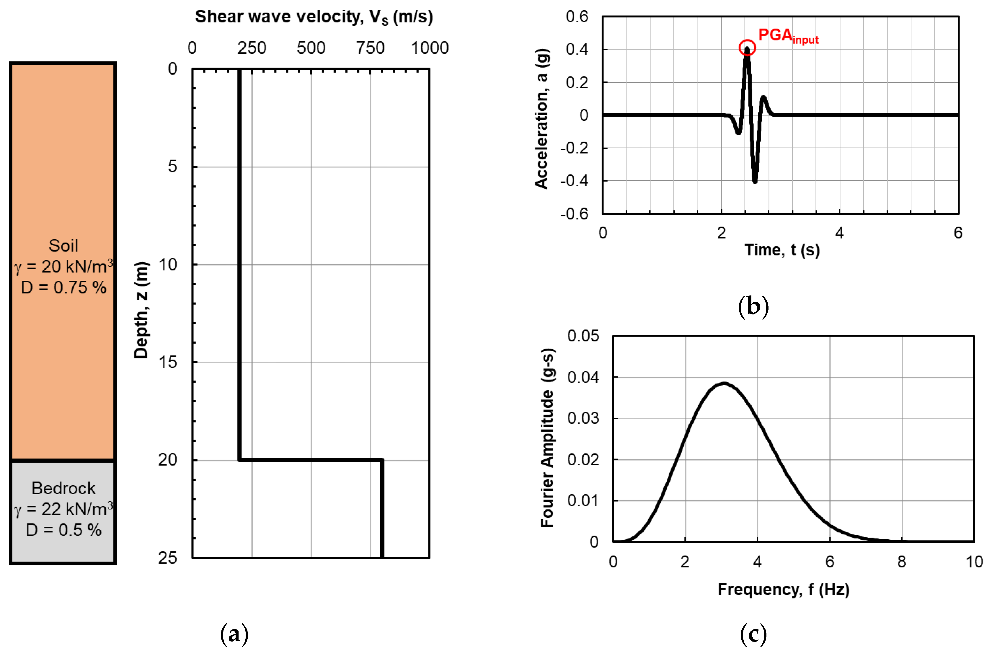
The first ideal model consists of a 20 m column of homogeneous soil assumed with a linear visco-elastic behavior (
Figure 3a). To test the performance of the code in the visco-elastic linear range of the soil, the visco-elastic linear analysis carried out with SCOSSA was compared to those of eight computer codes listed in
Table 1[
33]. The first five codes perform the analysis in 1D condition, while the remaining are among the most popular codes for 2D and 3D seismic response analysis used in professional practice.
The soil is defined by a unit weight of 20 kN/m3 and a shear wave velocity, VS, of 200 m/s, which remains invariant with depth. The dissipative behavior of the soil is defined by damping ratio, D, equal to 0.75%. This deformable layer rests upon a rock half-space that serves as the seismic bedrock. The bedrock exhibits a unit weight of 22 kN/m3, a shear wave velocity, VS, of 800 m/s and a damping ratio of 0.5%.
The soil column is subjected to an impulsive loading, similar to a Ricker-β wavelet type waveform, which is assumed to be recorded on a hypothetical rigid outcrop rock (outcrop motion). This motion reaches a Peak Ground Acceleration, PGA, of 0.4 g (
Figure 3b) centered on a frequency of about 3 Hz (
Figure 3c), which is in proximity to 2.5 Hz, i.e., the natural frequency of vibration of the soil column.
Details on the models as defined in the different adopted codes can be found in [
33].
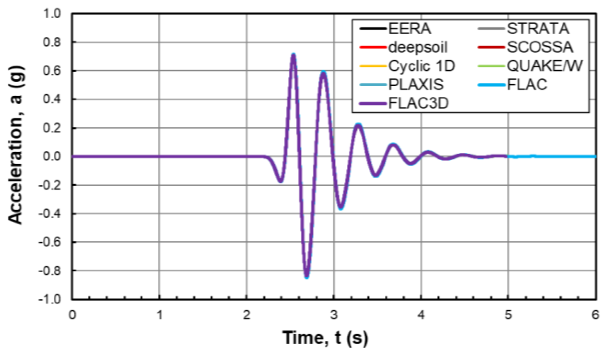
The comparison between the results of the simulations is expressed in terms of the time history of acceleration at the ground level (
Figure 4). The time histories of the acceleration at the surface show a perfect overlap among the different analyses.
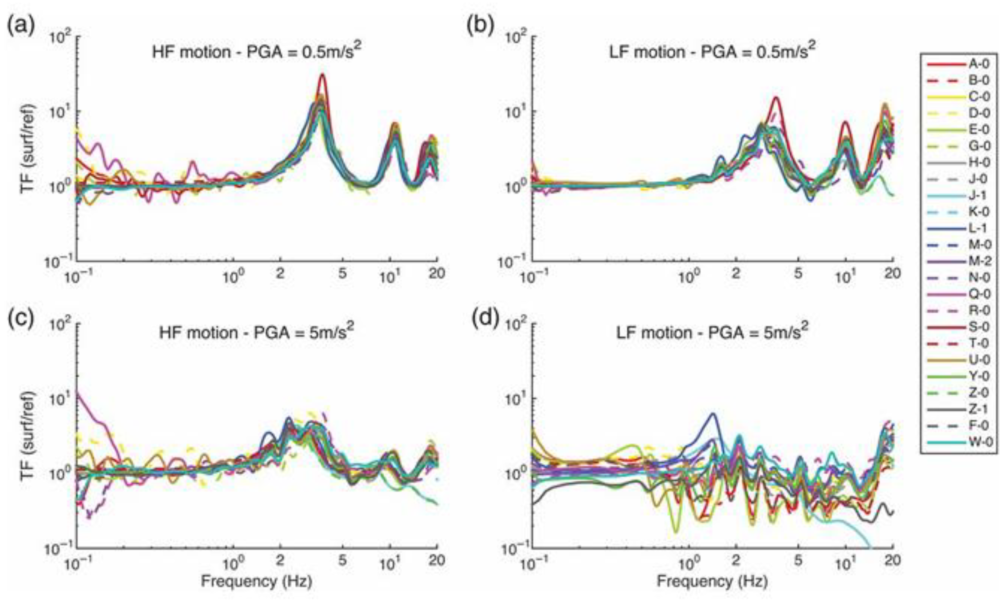
Similar results were also obtained in the framework of the international benchmark PreNoLin [
21] in terms of surface to reference Fourier spectra ratio for an ideal soil column (
Figure 5). Twenty-one collaborating teams evaluated twenty-three distinct numerical simulations, which incorporated more than ten different constitutive relationships [
21]. The organizing committee categorized the participating codes into three main, non-mutually exclusive groups, based on the following key attributes: 1) the numerical implementation scheme employed; 2) the damping mechanism formulation across both low-strain and large-strain domains; and 3) the formulation governing cyclic hysteretic response. A preliminary validation stage (i.e., cross-comparison among numerical codes) on simplified, idealized scenarios was conducted using 23 different codes, including the SCOSSA code, which is designated as ‘T-0’ in
Figure 5.
3.2.2. Validation on Case Histories
The validation of the code's performance within the low-to-moderate strain regime is proposed by referencing a seismic instrumentation array situated near Sendai port in northeast Japan. This data set was analyzed as part of the PreNoLin project [
22]. The monitoring station comprises a surface-mounted accelerometer and a downhole geophone positioned at a 10.4 m depth. The array is established within a Holocene sedimentary formation, termed the "beach ridge," which is composed of marine-origin gravel and sand. This surficial deposit overlies the Pliocene Geba Formation, which constitutes the northern and eastern hills and is characterized by gravel stone, sandstone, tuff, tuffaceous siltstone, and lignite [
7,
22].
The Sendai array location was chosen as a validation benchmark for the PreNoLin project primarily because the subsurface layering is demonstrably near-horizontal (as confirmed by multiple Multichannel Analysis of Surface Waves (MASW) tests), and the S-wave propagation vector of the selected seismic records is approximately vertical [
19].
The upper stratum of the soil column consists of loose gravel with a thickness of 1.25 m, which is underlain by 5.9 m of moderately dense fine sand. Below 7.15 m depth, a stiff slate formation is considered the seismic half-space. The phreatic surface is located at a depth of 1.45 m below the ground line. Downhole PS logging furnished the in-situ shear wave velocity profile, while the stress-strain and strength properties were determined via laboratory testing on undisturbed samples [
22,
42].
The shear wave velocity profile implemented in the analysis was obtained by calibrating the in-situ measurements until they exhibited optimal convergence with the empirical surface-to-borehole transfer function derived from weak-motion seismic recordings.
Undisturbed sand specimens were collected from depths of 3.3 m and 5.4 m for the purpose of executing laboratory experiments. Both samples were subjected to cyclic undrained triaxial tests to characterize the pre-failure stress-strain attributes of the soil. Furthermore, the cyclic and static strength parameters were measured on the shallower sample through stress-controlled cyclic undrained and consolidated-drained triaxial tests, respectively [
22,
42]. The cyclic liquefaction resistance and pore pressure generation parameters were subsequently assigned to the fine sand layer based on the findings from the cyclic triaxial liquefaction tests.
In the one-dimensional (1D) analyses conducted using the SCOSSA code, the downhole acceleration records were applied as the input excitation. Consequently, a rigid bedrock condition can be postulated at the 10.4 m depth, coinciding with the downhole sensor's location. Conversely, the slate rock stratum positioned above the downhole sensor (spanning 7.0 m to 10.4 m) was modeled as a linear visco-elastic material with a uniform damping ratio of 1%. Six recorded input motions with three distinct Peak Ground Acceleration (PGA) magnitudes (≥0.06 g, 0.02−0.03 g, and ≤0.01 g) and two differing frequency content categories were considered.
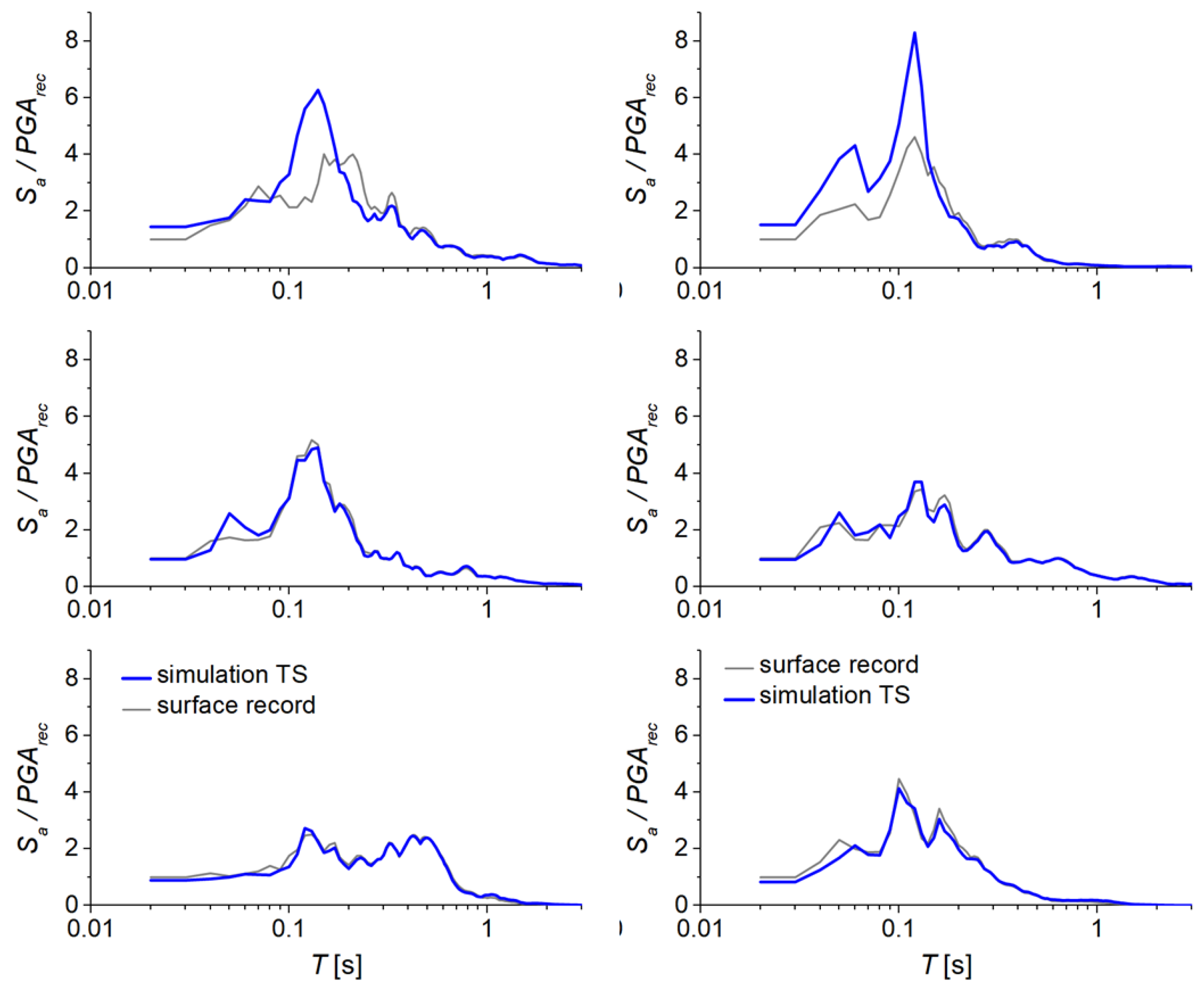
Figure 6 provides a comparative assessment between the surface records and the simulated outcomes from the total stress analyses for the low-frequency content input motions. The findings are presented as acceleration time histories and spectral accelerations, with both quantities normalized relative to the PGA captured at the surface.
4. Stick-Slip Model
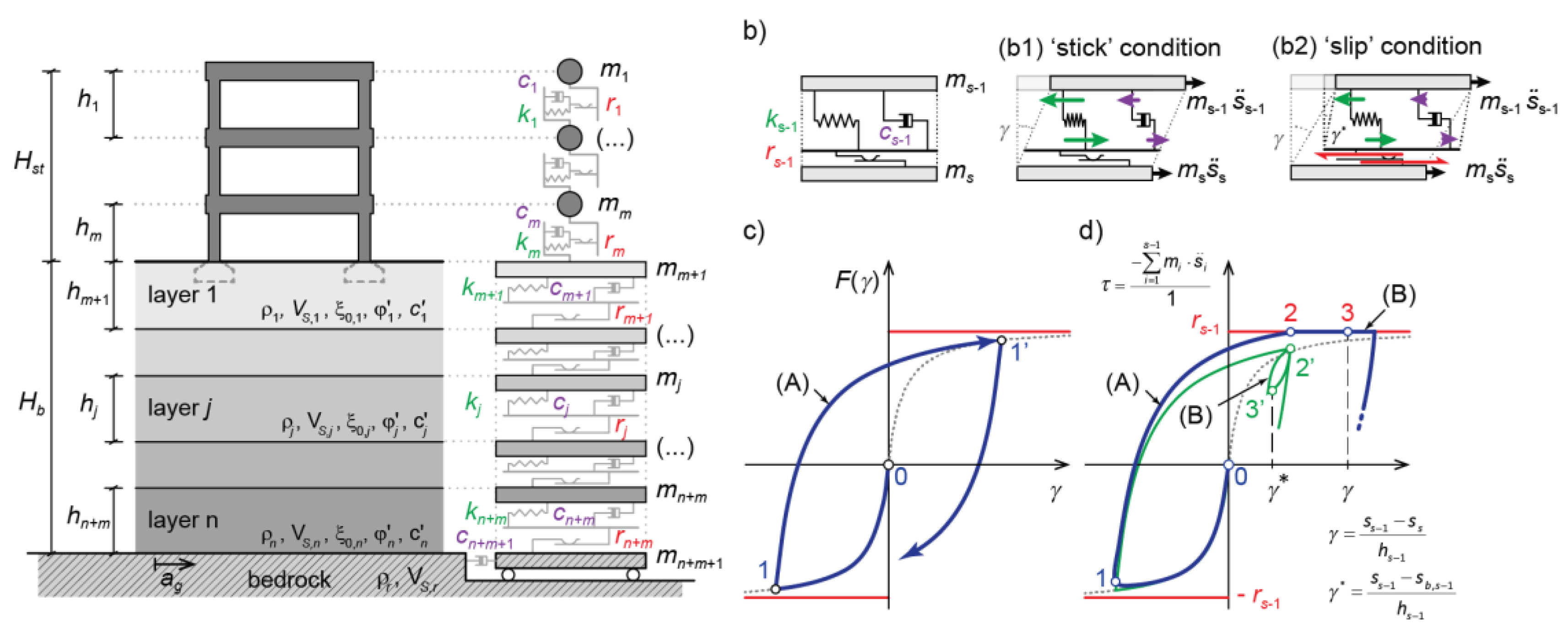
The dynamics of the stick-slip model implemented in SCOSSA refers to the lumped mass system sketched in
Figure 2 and then reproduced in
Figure 7a, where a plastic slider is added for each layer, which is activated when the limit tension
r is reached, thereby simulating layer breaking. The scheme can also include inclined layers to simulate an indefinite slope, or a frame overstructure modelled as an elementary oscillator, as shown in
Figure 7a (modified from [
19]). Two stages of analysis can be identified: in the ‘stick’ phase, the potentially unstable mass cumulates vibrational kinetic energy, which is transformed into a frictional sliding mechanism during the ‘slip’ stage.
In the stick phase, the seismic response in terms of absolute displacements can be computed by integrating the system reported in Eq. (1).
The vector of the applied forces depends on the input accelerogram, ag, which can be applied as ‘inside’ or ‘outcrop’ motion and on the bedrock impedance.
The shear critical strength at a possible failure surface can be expressed as
mT ay, where
mT is the total mass above the failure surface, and
ay is the yield acceleration, typically computed by the limit equilibrium methods. The forces acting on the sliding interface (
Figure 7) are:
The first term is the inertial force induced by the absolute acceleration at the s-th layer, , while the second is that resulting from the non-uniform relative acceleration profile, , within the sliding mass, referred to. The subscript “S” indicates sub-matrices and sub-vectors with index from 1 to (s - 1) for the sliding part of the dynamic system; 1 is the unity vector.
The ‘slip’ conditions start when the inertia forces equal the resisting force corresponding to the product of the sliding mass and the yield acceleration,
mT.ay. In such a case, the equation of motion for the deformable mass above the sliding surface is given by the expression:
On the sliding surface the equilibrium, during the slip, is governed by the condition:
Substituting eq. (5) in eq. (4), the equation for the ‘slip’ conditions is obtained as:
where
M* is defined as:
Solving eq. (6) in terms of nodal relative acceleration,
, the sliding acceleration time histories are obtained from eq. (5) as:
The sliding displacement, s0, is computed by integrating twice eq. (21) until the sliding velocity becomes equal to zero.
Figure 7b illustrates the performance of the constitutive model for the generic (
s-1)th layer immediately above the sliding surface. The masses
s-1 and
s are connected by a non-linear hysteretic spring (
ks-1), a viscous dashpot (
cs-1) and a plastic slider (
rs-1). Under static load, the MKZ model uses two relationships:
Fbb(γ) for first loading (e.g. 0 → 1 in
Figure 7c) and
Fur(γ) for unloading-reloading paths (e.g. 1 → 1’ in
Figure 7c). The limiting strength is reached asymptotically when MKZ model degenerates to the hyperbolic stress-strain relationship. In dynamic ‘stick’ conditions (see pattern b1 and the corresponding point on the reloading curve in
Figure 7d), the current value of shear stress, τ, is computed considering the dynamic equilibrium of soil column (Eq. (1)). As a consequence, the γ - τ relationship deviates from the purely hysteretic response (dashed line in
Figure 7d), shows rounded edges (point 1) and possibly reaches the limit strength (point 2) attaining the ‘slip conditions’ (pattern b2 in
Figure 7b). Thereafter, the shear stress holds constant until the system accumulates plastic straining, while the hysteretic response of the spring results into a small unloading-reloading cycle (
Figure 7d), induced by the application of modified Masing rules. Due to slippage, the subsystem above the sliding base is characterized by an actual value of the shear strain in a generic instant (indicated as γ* in
Figure 7b,d) lower than the total strain, γ.
Different options are implemented into the code for the position of critical sliding surface, Hs, which can be either imposed before the analysis or it can be automatically sought by identifying the layer where the slippage condition is tested out for the first time.
The stick-slip was verified on a dam and a landslide case study as reported in [
20].
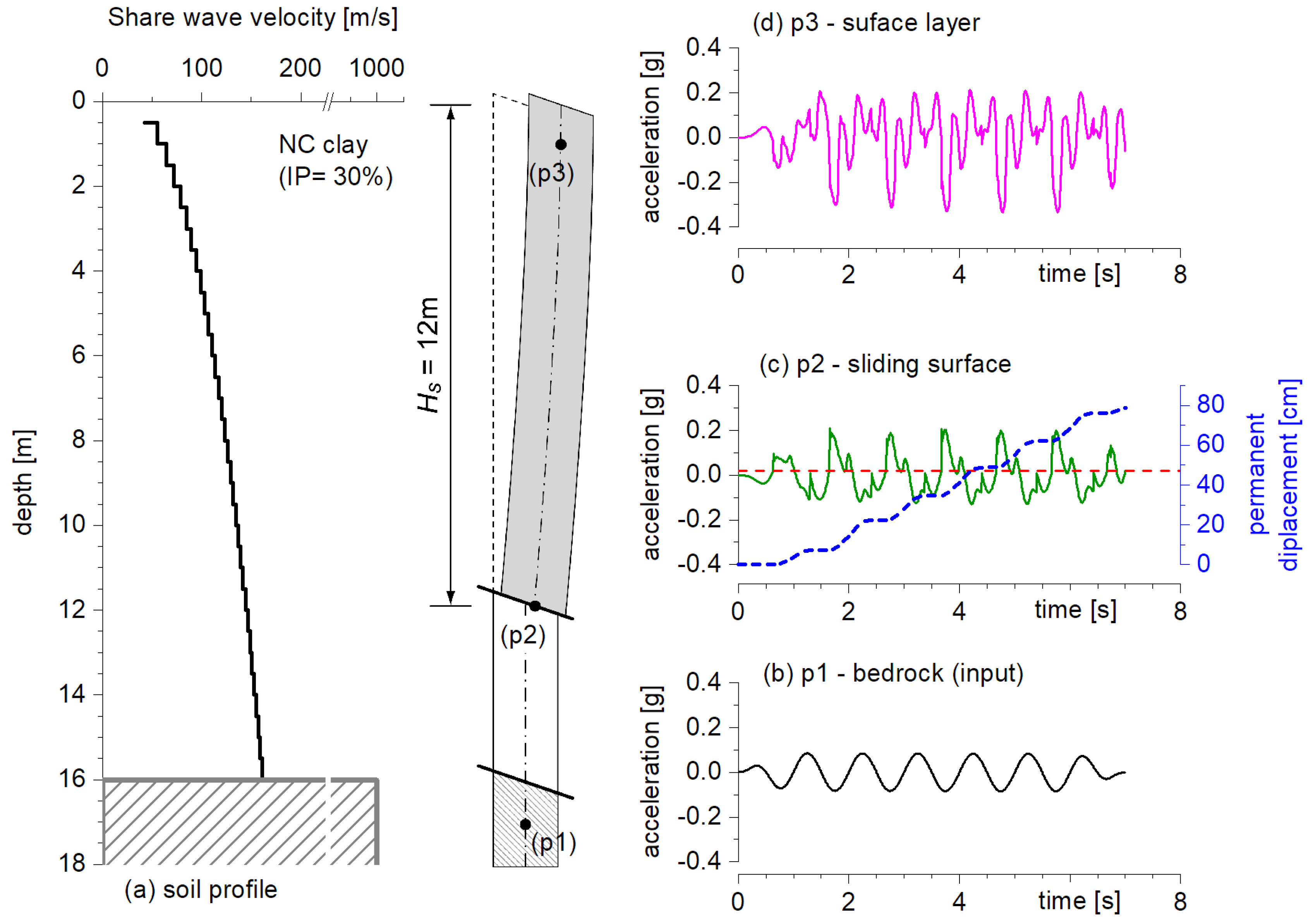
Figure 8 shows the results of a theoretical exercise modified from [
19]. The soil, is a normally consolidated, medium-plasticity clay layer (IP = 30%) with a unit weight equal to 19 kN/m
3 and a
VS profile that increases with depth (
Figure 8a). The soil is characterized by cyclic hysteretic behaviour defined by the Vucetic and Dobry curves [
43]. The critical acceleration value of 0.017 g is depth-independent due to the combination of soil resistance, as defined by the Mohr-Coulomb failure criterion, and the gentle slope of the layers.
The input motion considered at the bedrock layer (p1 position in
Figure 8b) is a sine wave with amplitude 0.1g, frequency 1 Hz, and duration 7’ (equivalent to 7 cycles), with the first and last ones modulated in amplitude with two sigmoid laws. In
Figure 8c and
Figure 8d the results obtained at the first detected sliding surface depth (p2) and at the layer surface (p3) are shown. In detail of acceleration time history and cumulated displacements at the sliding surface layer to explain what occurs during the stick and slip phases.
At the time
t = 1.3 s, the unstable mass, which has cumulated about 5 cm from the previous slip phase, is in stick condition until a new triggering of motion occurs at the time 1.7s (
Figure 8c). During this lapse, the soil can respond to dynamic input with upstream instantaneous displacements. Starting by
t = 1.7s, a new slip stage with a graduate increase of displacement along the sliding surface occurs. As can be seen in the results shown in
Figure 8c and
Figure 8d, the slip at the base of the column causes the freely oscillating system to respond with a higher natural frequency than the non-sliding system. High-frequency oscillations resulting from numerical errors in the transition between phases are also observed. This oscillation propagates to the surface at the same frequency, displaying a clearly asymmetric amplitude signal.
5. Liquefaction
The seismic response analysis of saturated soils is a complex process governed by two key phenomena: hysteresis and volumetric-distortional coupling. Hysteresis involves a reduction in shear modulus and increased damping and volumetric-distortional coupling gives rise to irreversible plastic strain under high shear loads, which can lead to liquefaction in loose sands.
Although hysteretic effects are widely modeled, volumetric-distortional coupling remains a challenge. Two primary approaches are used to model pore water pressure variation:
The coupled approach can be further divided into:
loosely coupled: predicts pore pressure using relationships combined with total stress constitutive models [
45].
fully coupled: uses a plasticity-based constitutive model to simultaneously predict both stress-strain and pore pressure. Particularly popular in the last decades are the multi-yield surface models (e.g., [
37,
46]) and the bounding surface models (e.g., [
47,
48]).
For the implementation in the code, a simplified stress-based pore water pressure model was considered. This model takes a loosely coupled approach, which makes it practical because it can handle irregular shear stress time histories directly, removing the need to calculate an equivalent number of uniform stress cycles - a common requirement for other simplified models (e.g., [
49]). The model also avoids the complex parameter calibration required by more advanced plasticity-based approaches. This makes it a valuable tool in engineering practice, as it requires only a few easily calibrated parameters. The model also accounts for stiffness and strength degradation due to pore pressure build-up, considering the redistribution and dissipation of excess pore pressure based on one-dimensional consolidation theory.
The following reasons drove the choice of this model over the plethora of possible options: 1) the simplicity of the model which is ruled by few analytical relationships; 2) the consistency of the model with the worldwide-accepted liquefaction framework based on the cyclic resistance curve of soils, i.e., stress-based approach; 3) the feasibility in implementing the model in a time domain integration algorithm; 4) the straightforward quantification of the model parameters through soil testing.
Concerning the last point, the calibration of the simplified pore water pressure model, originally developed on the results of cyclic laboratory tests, was then expanded to the results of the Cone Penetration Test, Standard Penetration Test, and seismic dilatometer test [
10,
11]. However, these calibration procedures attempt to reproduce trends experimentally observed, without a rigorous connection with the soil mechanics theory. Additionally, different pore pressure curves belonging to the same soil but with different relative density require independent calibrations of the model parameters.
Modifications to the basic numerical procedure of the code, as reported in section 3, were necessary in order to implement the pore pressure generation and dissipation models.
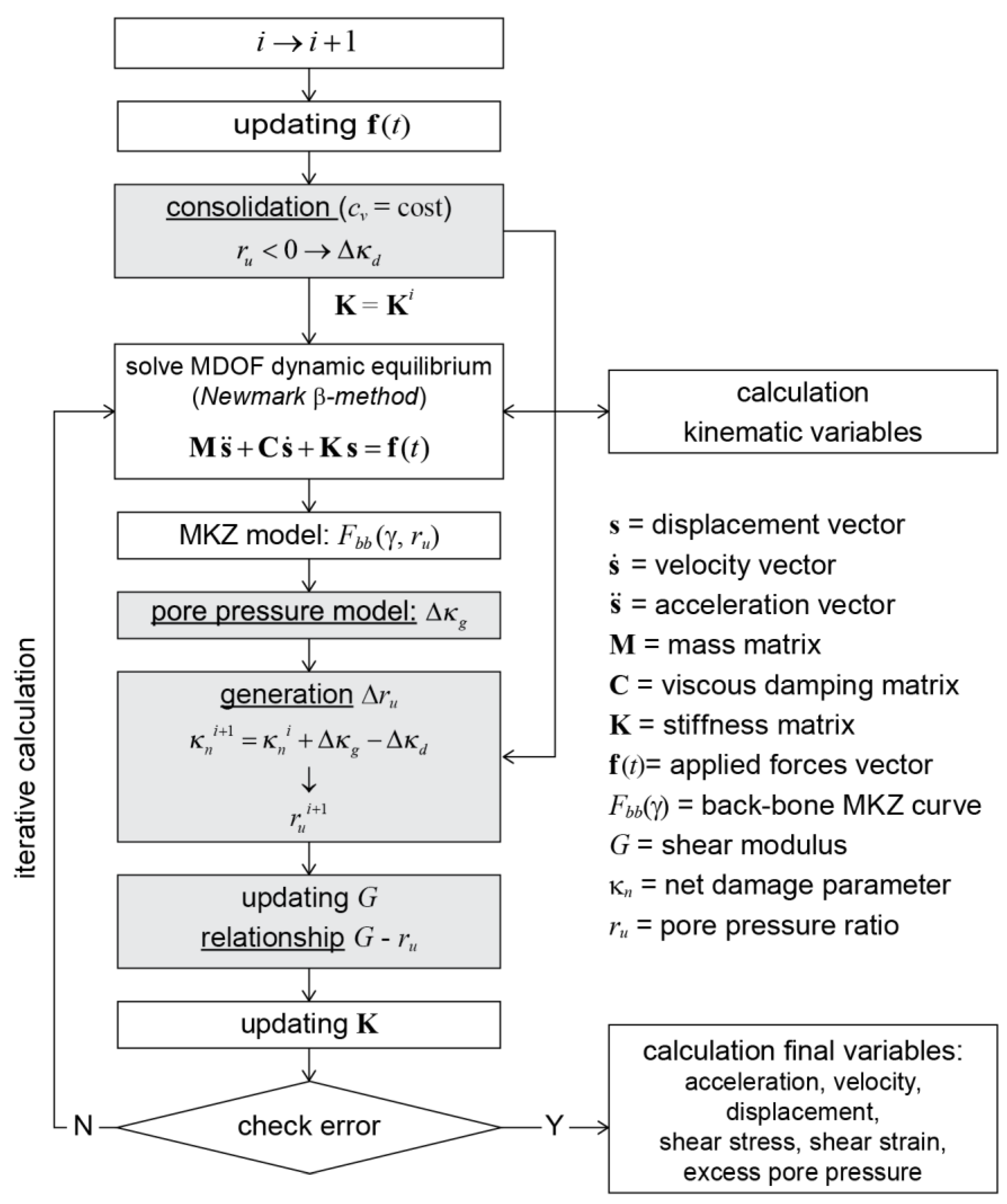
Figure 9 shows the flowchart outlining the schematic algorithm adopted in the SCOSSA-PWP code for each time step.
Novel modules have been integrated into the original SCOSSA algorithm, encompassing routines for consolidation, pore water pressure generation, and shear modulus adjustment (indicated by the shaded boxes in
Figure 9). A comprehensive explanation of these specific routines is reported in the following.
According to the flowchart in
Figure 9, an initial updating of the vector of input forces,
f(
t), is carried out for the
i-th time step. During the same time interval, a new distribution of the pore water pressure along the soil profile is evaluated, starting from the distribution evaluated at the previous time instant, assuming a constant value of the consolidation coefficient. The consolidation induces a decrease in the excess pore water pressure, with a negative variation in the pore pressure ratio,
ru; this variable is defined as the ratio between the pore pressure, Δ
u, and the initial effective stress of the soil, σ’
0 (vertical stress in cyclic simple shear or mean effective stress in different conditions).
The cyclic response model (Eq.
Error! Reference source not found.) is modified by including the degradation index functions
δτ and
δG. The modulus degradation index function,
δG, is defined as:
while the corresponding stress degradation index function, δτ, is given by:
where μ is an exponential constant that expresses the sensitivity of the backbone curve to pore water pressure changes. Matasovic and Vucetic [
29] defined the constant μ based on the stress-strain response obtained from strain-controlled cyclic simple shear tests on Californian sandy soils. They found μ values ranging between 3.5 and 5. The same direct relationship between shear modulus and excess pore water pressure is also frequently used in other codes suitable for effective stress analyses (e.g., D-MOD2000 [
50]).
The above degradation index was also used for expressing the stress-strain relationship in unloading-reloading conditions, according to the relationship proposed by Moreno-Torres et al. [
51]. As a consequence, Eq. (13)and (14) are modified as follows:
5.1. PWP Model
The selected model belongs to the family of the endochronic models [
52,
53,
54,
55,
56,
57]. It is based on the definition of the “damage parameter”, κ, that summarizes the effect of the cyclic variation of stress/strain on the undrained soil response. This parameter is an increasing variable during the loading history that can be directly correlated with the pore pressure accumulation as follows:
The pore pressure model also defines a univocal relationship between the normalized damage parameter, κ
/κ
L, and the pore pressure ratio,
ru, through the polynomial [
8]:
where
a,
b,
c and
d are the curve-fitting parameters.
The endochronic-based damage parameter, κ, permits avoiding the use of non-univocal criteria to convert the irregular shear loading into an equivalent number of cycles [
58], sometimes characterized by quite challenging procedures [
59,
60,
61].
For a regular harmonic loading of given amplitude, CSR, i.e., the ratio between the modulus of the maximum shear stress, |τ
max|, and the initial effective stress, κ is proportional to the number of cycles,
N, and can be written as:
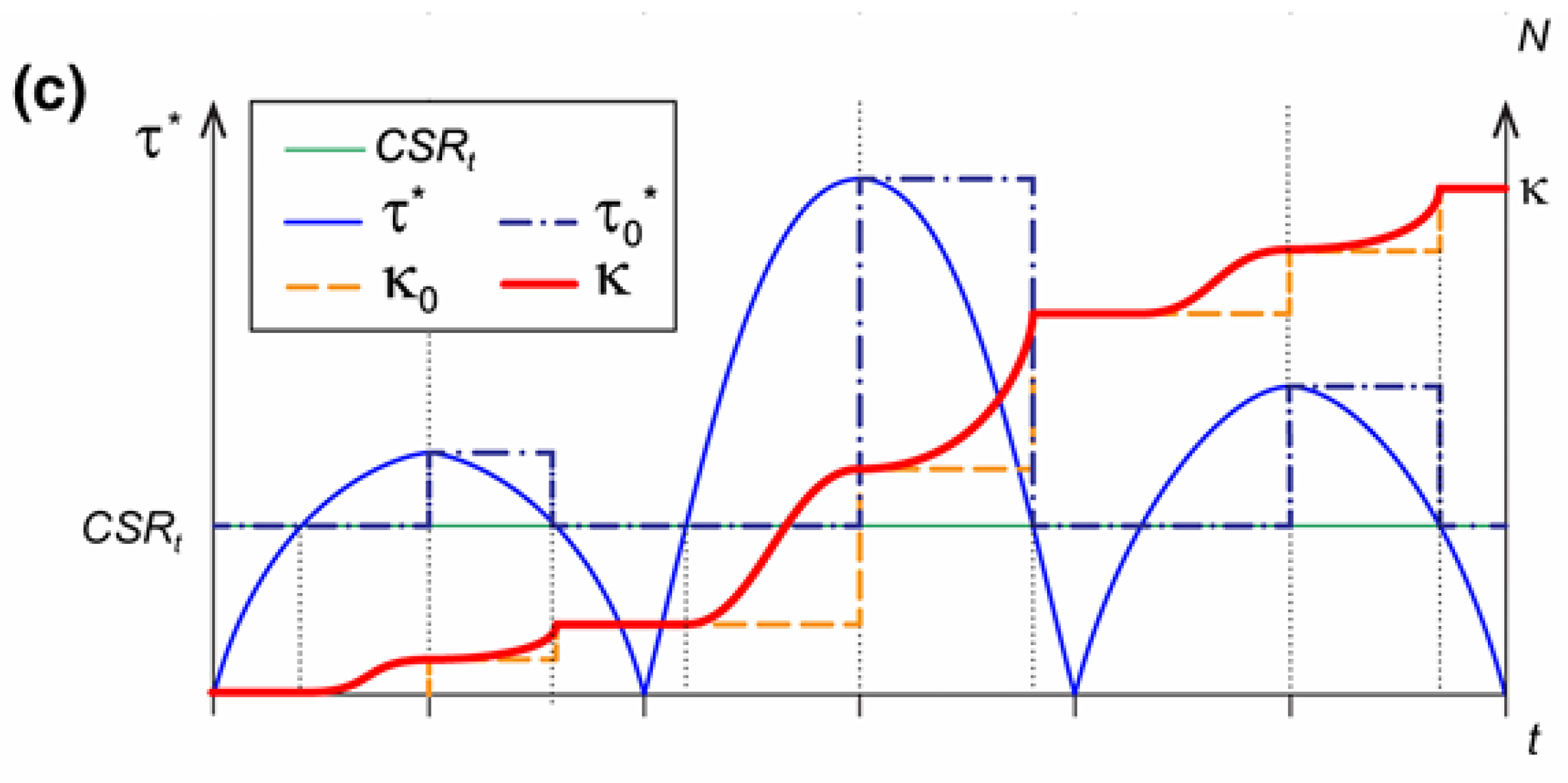
For an irregular shear loading history (
Figure 9), expressed as follows:
The damage parameter can be computed at every time instant as:
where κ
0 is the damage cumulated at the last reversal point of the function (τ* - CSR
t) reached at the time instant,
t. The parameter κ
0 can be defined as follows:
i.e., κ
0 is a stepwise function assuming the value of the damage parameter gained at the time step (
t −
dt) every time the stress ratio reaches a local maximum value or when
τ* = CSR
t.
The increment of the damage parameter,
dκ, in the time interval dt is given by:
The damage function increases when
τ* overtakes CSR
t, the threshold below which there is no pore pressure build-up (
Figure 10).
In the discrete time step analysis, it is possible to define the “generated damage” increment, Δκ
gen, as follows:
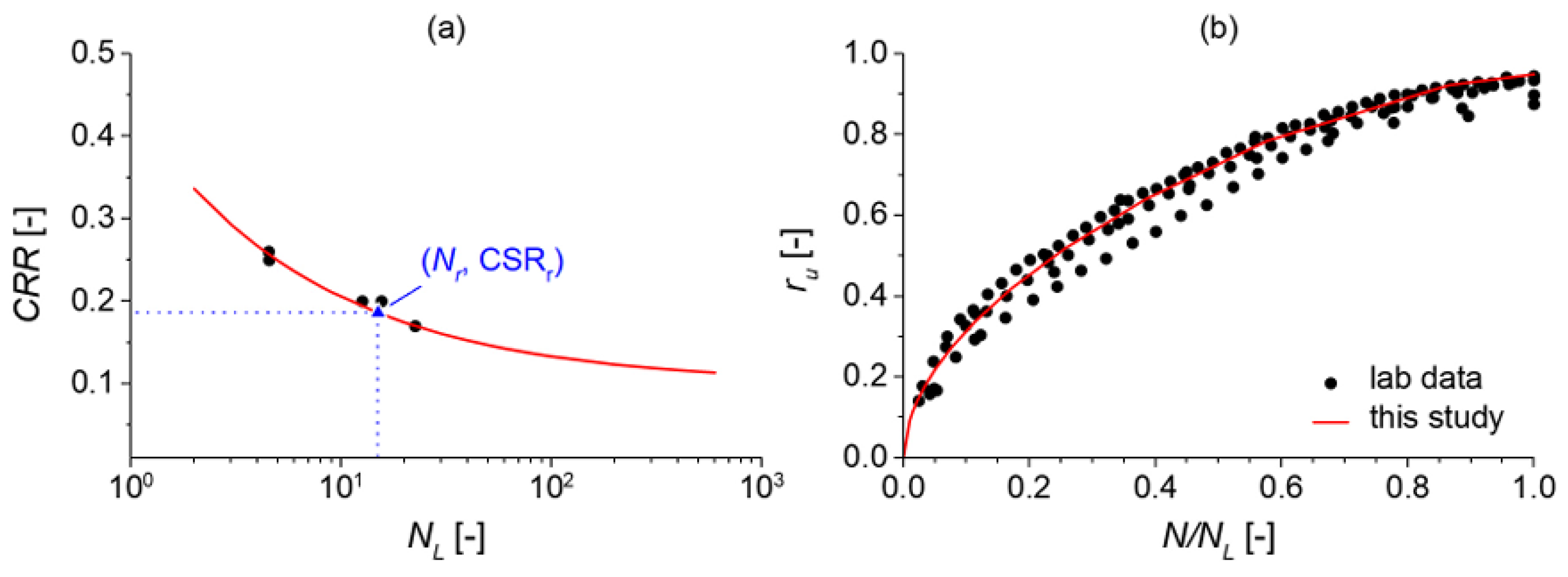
The analytical expressions for the cyclic resistance curve CRR : N
L is generally based on a power function [
62,
63,
64]. The one considered in SCOSSA-PWP is that proposed by [
56,
65], which is rewritten as follows:
where (
Nr, CSR
r) is a reference point on the cyclic resistance curve, and the exponent α describes the dependency of the cyclic resistance on the number of cycles (
Figure 11a).
Combining Equations (34) and (28) for CSR equal to CRR, the damage parameter at liquefaction, κ
L, is expressed as follows:
The relationship (35) shows that damage at liquefaction assumes a constant value depending on the parameters describing the cyclic resistance curve, α, CSR
r and CSR
t. Therefore, any point on the cyclic resistance curve is associated with the same damage level, κ
L; furthermore, in the
N - CSR plane, it is possible to draw different “iso-damage” curves, which express at any value of CSR the number of cycles necessary to obtain a damage corresponding to a given percentage of κ
L [
8].
The normalized damage, defined as the ratio between the damage, κ, and that evaluated at liquefaction, κ
L, is defined as follows:
Combining Equation (36) and Equation (27), the normalized damage is equal to the ratio between the generic number of cycles and the number of cycles at liquefaction,
NL, as shown in the following (Fig 11b):
Suggestion for calibrating model parameters using laboratory data are reported in [
8,
24], particularly concerning defining the asymptotic value of the cyclic resistance curve, CSR
t, which is not always clearly identifiable from experimental data.
One of the main challenges in performing effective stress analysis is calibrating a constitutive model that can simulate dynamic soil behavior under seismic loading. To address this issue, a calibration procedure has been developed to define parameters for advanced constitutive models based on data from in-situ tests, such as cone penetration tests (CPT) and standard penetration tests (SPT). Ntritsos and Cubrinovski [
66] generated a dataset of cyclic resistance curves based on the liquefaction triggering semi-empirical methods, and, then, used the dataset for calibrating an advanced constitutive model [
67,
68]. Following the above-mentioned approach, the calibration of simplified stress-based pore pressure models, which was initially based solely on cyclic laboratory test data, was extended to include results from field tests commonly used in engineering practice [
10,
69].
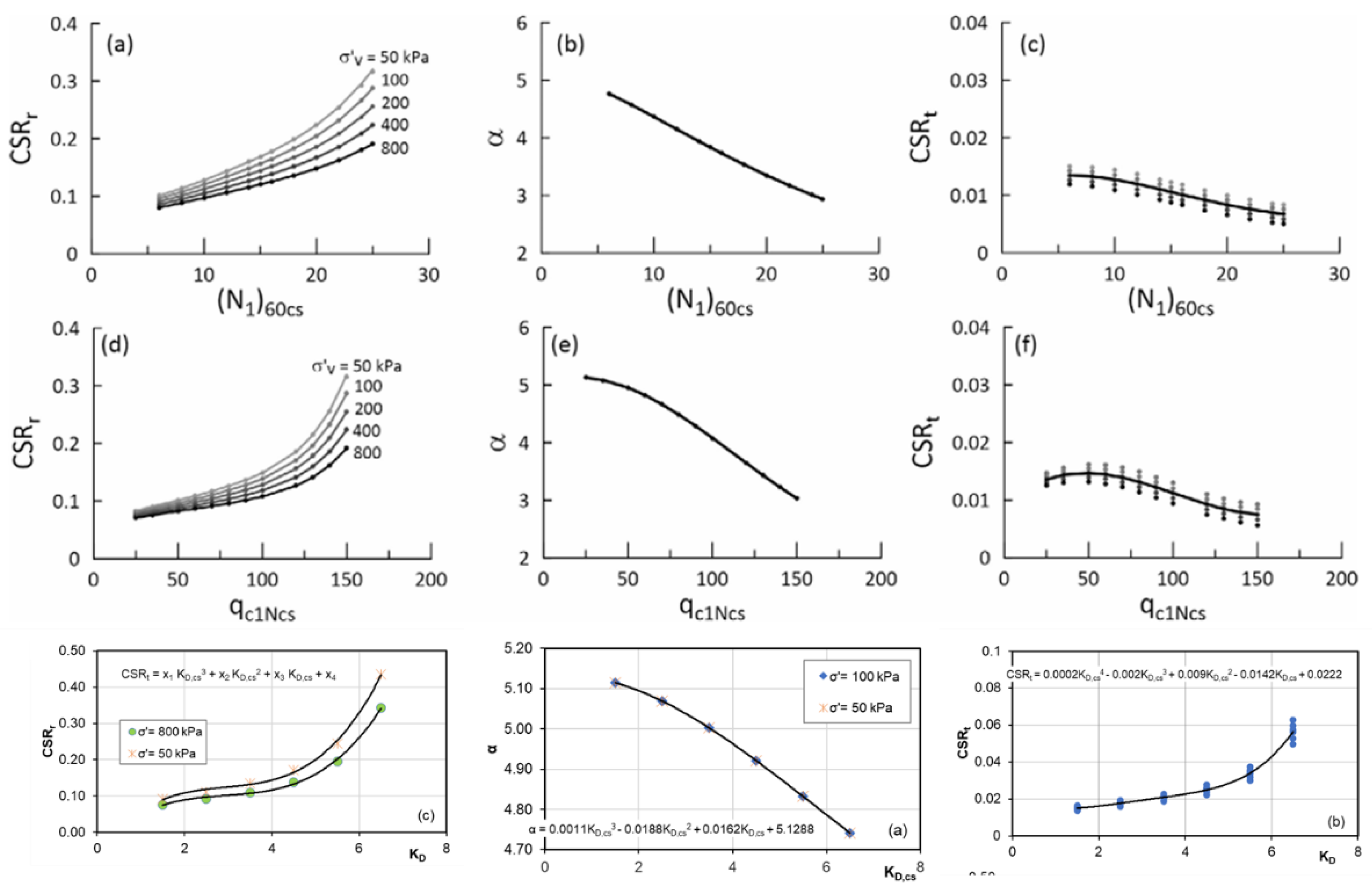
More recently, the DMT-based calibration was upgraded by [
11] to incorporate the effects of the fines content on the behavior of granular soil mixtures as proposed by Chiaradonna and Monaco [
70].
Figure 12 shows the CPT, SPT and DMT-based charts for calibration of the PWP model parameters necessary for the definition of the cyclic resistance curve (Eq. 34).
In
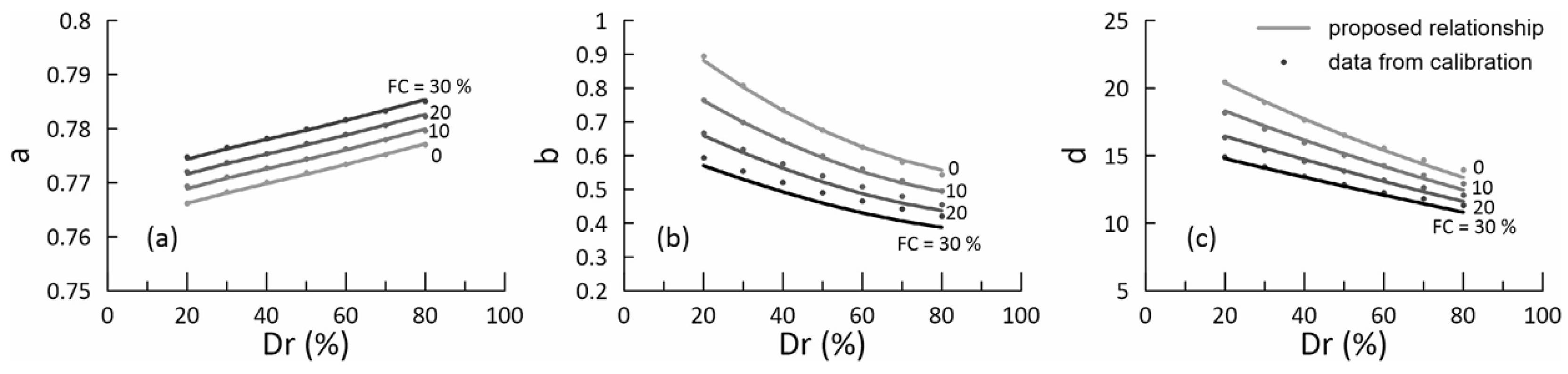
Figure 13 the pore pressure parameters are plotted as a function of the fines content and relative density. More recently, de Cristofaro et al. [
71] show the dependency of the mechanism of excess porewater pressures on the stress history, stress state, and stiffness of soils by using two key parameters, ψ and λ, derived from the steady-state theory. Consequently, the pore pressure parameters (Eq. 37) were correlated to the state parameters for two pyroclastic soils, experimentally investigated with cyclic triaxial tests.
5.1. Review of Applications and Case Studies
The performance of ‘SCOSSA PWP’ in predicting pore water pressure build-up and dissipation has been validated against data from seismic centrifuges [
7,
12,
13] and instrumented field sites [
7,
10,
12]. Comparisons with more complex codes on real and ideal cases [
14,
15], including the numerical benchmark LICORNE [
72], have also been performed.
Furthermore, post-analysis results have been used to predict both horizontal displacements and post-consolidation settlements in real-world case studies, with estimates aligning well with observed damage [
12,
17,
73]. Further applications to case studies have been performed for investigating the effect of unsaturated soils on cyclic strength [
74,
75] and investigating possible sources of damage in liquefaction sites, such as Pieve di Cento [
76] and others [
77,
78].
To illustrate the types of analyses that the code can handle, total undrained effective stress analyses are reported in the following. Specifically, the Sendai and Port Island vertical array case studies are shown to show the analyses in totally undrained effective stress. The dissipation and redistribution of excess pore water pressure are challenging phenomena to be analyzed in a real case study, so several physical models have been carried out in centrifuge tests to gain insight into liquefaction mechanisms [
79,
80,
81,
82]. These tests have been used as a reference for validation of advanced constitutive models and codes [
83,
84]. Similarly, the code performances in partially drained effective stress analyses are shown in the following for the numerical simulations of centrifuge tests
5.2.1. Validation on Sendai Case Study
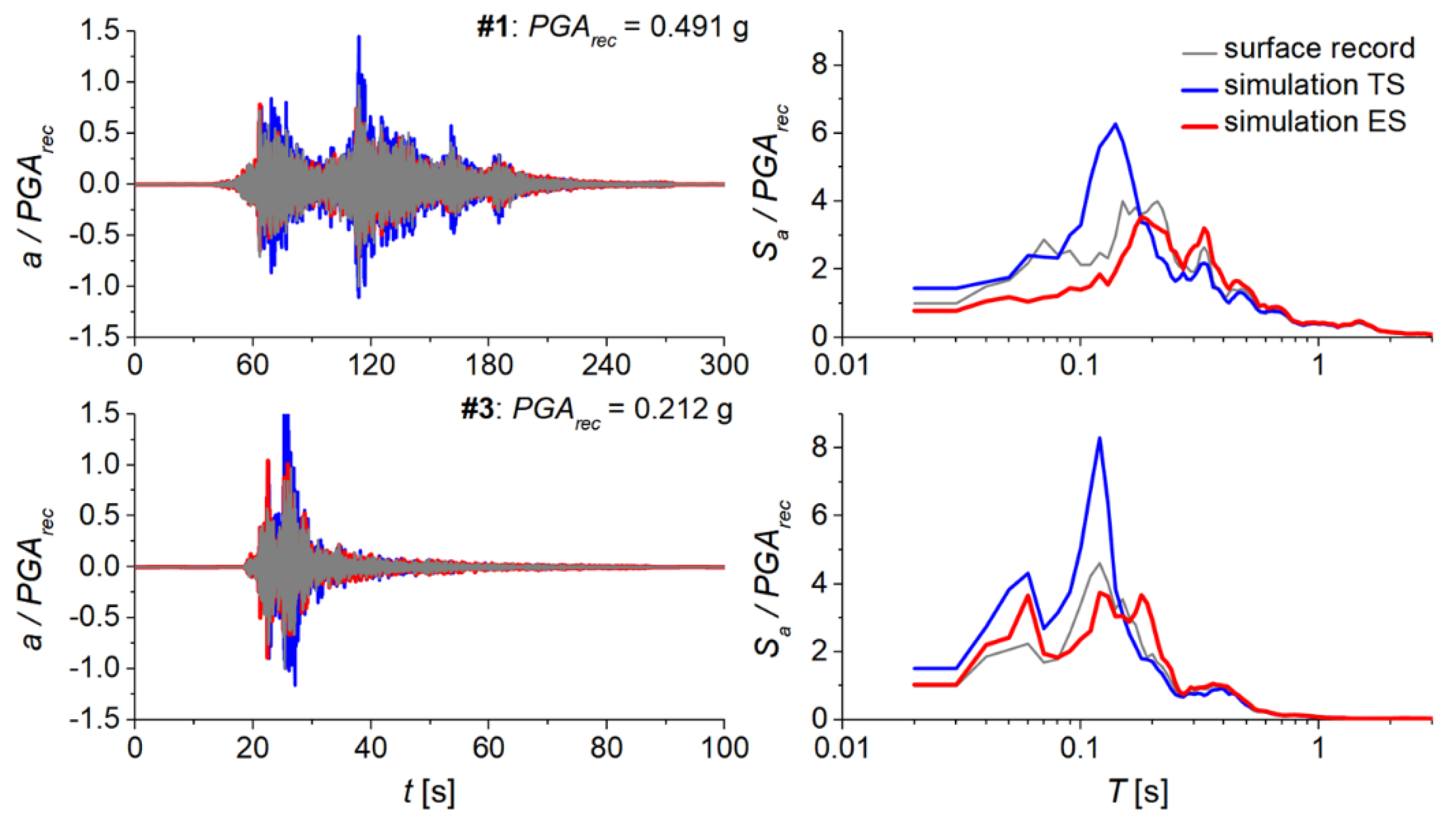
The simulations reported in section 3.2 were repeated under effective stress conditions. Although the entire set of input motions listed in section 3.2 was considered, excess pore pressure was only triggered for records #1 and #3 (i.e., those with the highest PGAs, at 0.257 and 0.062 g, respectively). For all the other input motions, the results of the effective stress analyses coincide with those shown above.
The results of effective stress analyses for input motions #1 and #3 are compared in
Figure 14, with the recorded data and the results of total stress simulations. The comparisons demonstrate that effective stress analyses predict the surface ground motion with satisfactory reproductions of the maximum recorded spectral accelerations and predominant periods.
5.2.2. Validation on Port Island Case Study
Port Island is a well-known example of liquefaction on reclaimed ground used by several research groups to validate liquefaction models [
85,
86,
87,
88,
89]. Following the 1995 earthquake, various locations on the artificial island showed clear signs of liquefaction [
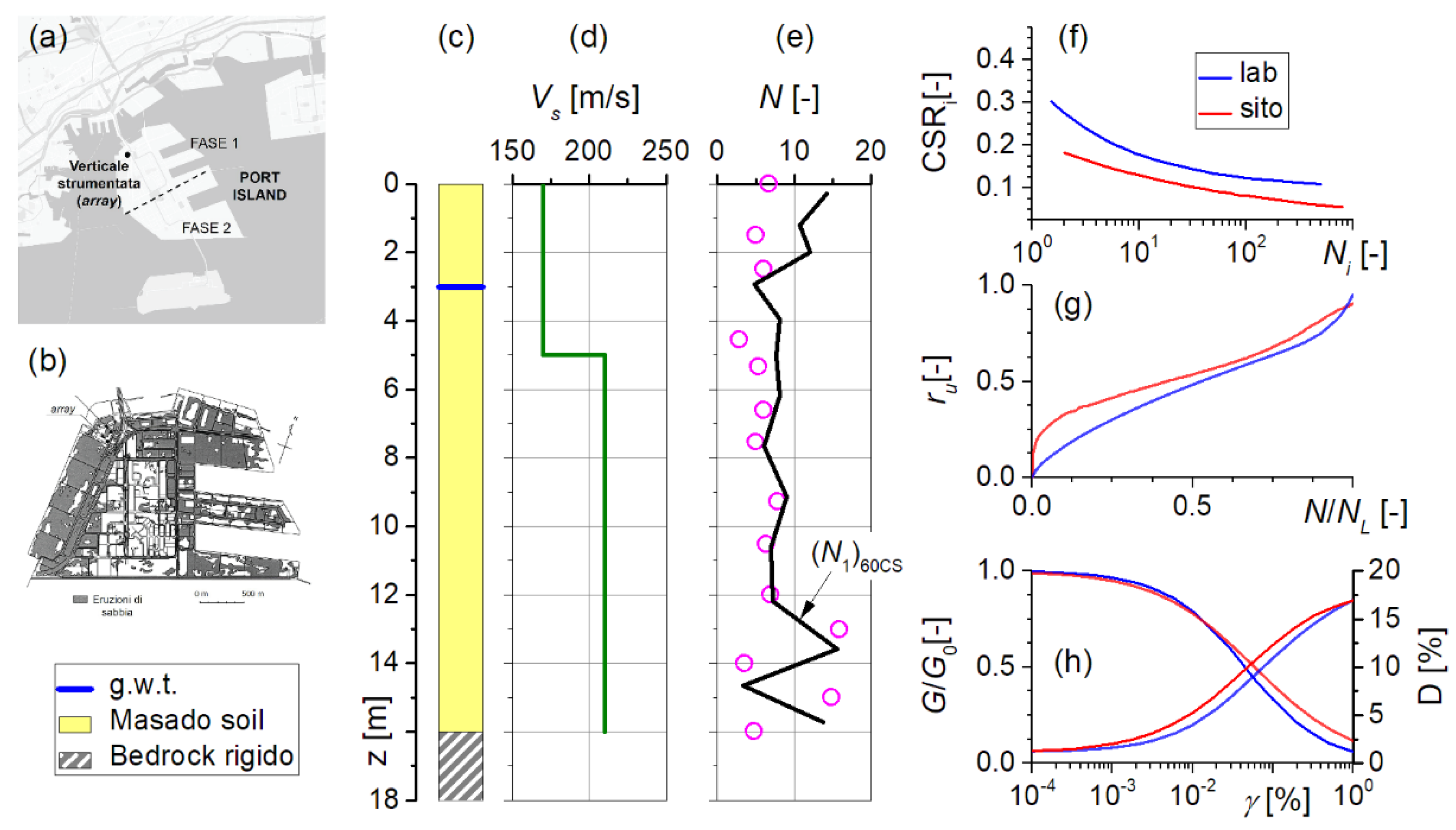
90]. Port Island was the first man-made island to be built in Osaka Bay, south of Kobe City. The construction of the island was undertaken in two phases. The initial phase of reclamation utilized soil comprising decomposed granite, known as "Masado", whereas the southern reclamation employed sandstone, mudstone, and tuff.
The 1995 Hyogoken-Nanbu earthquake, which had a local magnitude of 7.2, impacted the southern portion of Hyogo Prefecture. The hypocentral depth was determined to be 14.3 km below sea level, with the epicenter located 15 km north of Awaji Island. Liquefaction occurred extensively throughout the island. The mean settlement was found to be 20 cm, with peak values exceeding 50 cm in the areas most severely impacted. According to the testimony of witnesses, the process of ejection of liquefied materials on Port Island continued for approximately one hour in the aftermath of the earthquake. The ‘Masa’ or ‘Masado’ soil constitutes the superficial sandy layer, the decomposed granite transported from the nearby Rokko Mountains, overlying a Holocene silty clay layer. Below these layers, alternate layers of Pleistocene gravel and clay can be found. The Masado soil is well graded, containing approximately 55% gravel and exhibiting a relative density of 47% for the silty sand portion of undisturbed samples. The groundwater table is located at a depth of 3 m below the surface, while the bedrock is situated at a depth of 16 m.
Figure 15 shows the normalized shear modulus,
G/
G0 and damping,
D, curves used in the investigation. The shear modulus reduction and damping curves reported in
Figure 15h were used to capture the Non-Masing behaviour. The input motion was provided at the base of the soil column.
Since the ejection of liquefied materials on Port Island persisted for about an hour [
90], the dissipation of the excess pore water pressure is not considered during the time of the shaking and the analyses are performed in totally undrained conditions.
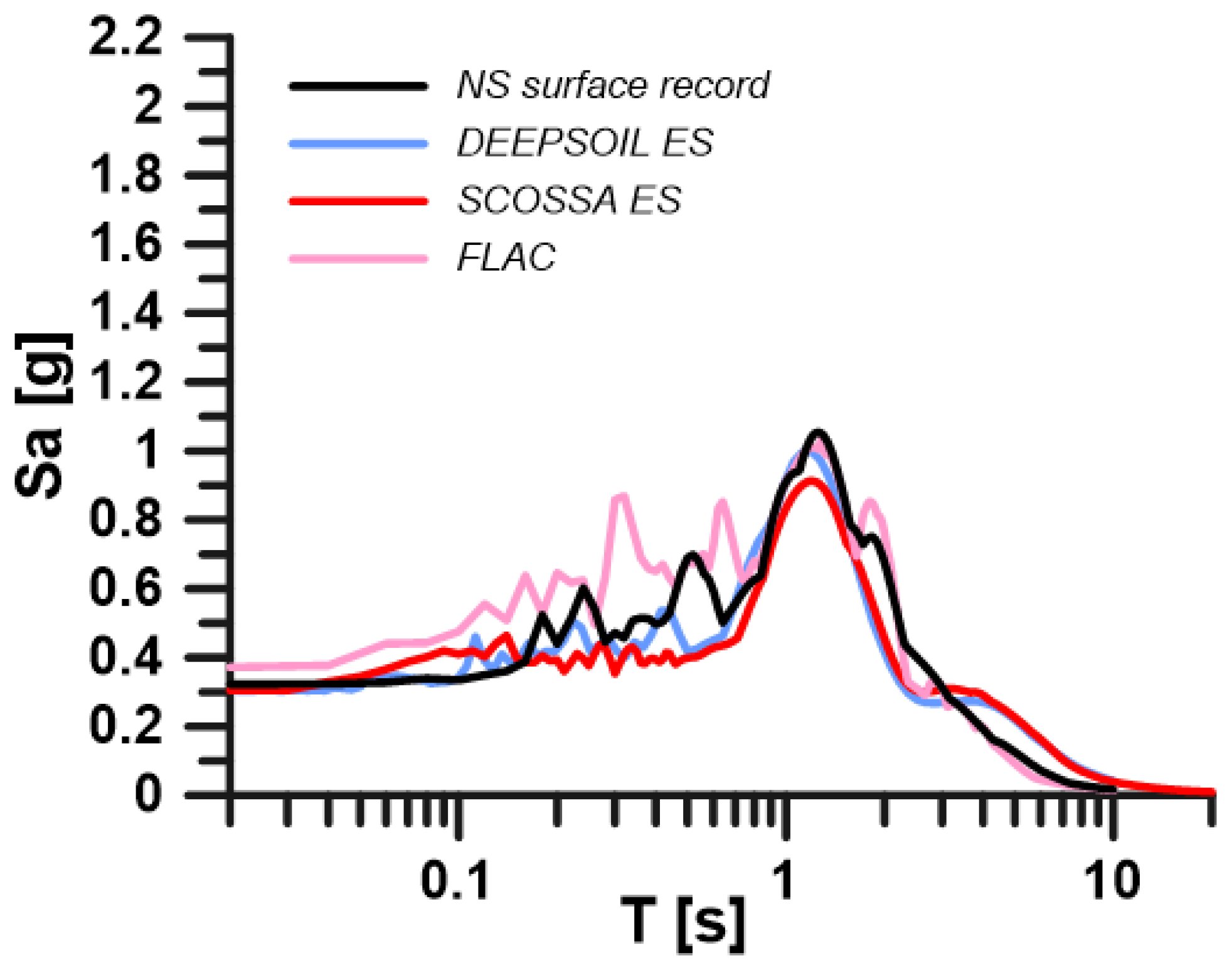
The simulation of the soil response at the array site has been performed with SCOSSA and DEEPSOIL [
36]. For the two codes, the same parameters were considered except for the pore water pressure model. In DEEPSOIL, the Dobry/Matasovic model was selected, and the parameters were calibrated according to the Carlton [
91] procedure as detailed in Paul et al. [
92].
This Dobry/Matasovic model for sand was initially proposed by Dobry et al. [
93], and it has been updated by various researchers [
94]. The formula below is used to estimate excess pore water pressure:
Where: Neq is the equivalent number of cycles for the most recent reversal of strain and it is set equal to the number of cycles for loading. Since the cycle number is irregular for strain cycles, Neq is determined at each strain using a 0.5-increment. The volumetric threshold shear strain is ɣtvp. When the shear strain level exceeds the threshold shear strain value, the excess pore water pressure is different from zero.
Vucetic and Dobry [
94] introduced the parameter
f for the purpose of modelling the cyclic loading in various dimensions. The value of
f is equal to 1 in 1D motion and 2 for 2D motion. The fitting curve parameters,
F,
s, and
p are calibrated by using the results of laboratory tests. However, empirical correlations for the curve fitting parameters
F and
s for sands have been proposed by [
91] according to the following expressions:
where FC is the fines content (in percentage) and
Vs is the shear wave velocity in m/s.
The same column was analysed by [
95,
96] adopting the advanced constitutive model PM4Sand [
97] for the modelling of the Masado soil, starting from the calibration work performed by [
98]. Details on the model and calibration procedure are here omitted for sake of brevity, but the reader can find them in [
95,
96].
The results of the effective stress analyses in terms of acceleration response spectrum are compared in
Figure 16, for the NS component.
5.2.3. Validation Against Centrifuge Test Results
The first centrifuge experiment considered in the simulation is the Centrifuge test No. 1 from the VELACS project [
99]. In this case, a 10m-thick layer of Nevada sand with a 40% relative density was placed in a laminar box to simulate a semi-infinite soil layer. The box, which allows for soil deformation, was spun at 50 g and shaken horizontally. Sensors measured horizontal and vertical accelerations and pore pressures.
The model consisted of a 10 m-thick uniform sand layer with an impervious base and a groundwater table at the surface. The dynamic properties of the sand were defined using resonant column tests, linking small-strain stiffness.
The cyclic resistance and pore pressure relationships were also determined from laboratory tests [
100]. A key aspect of the numerical simulation was using a unit weight of 25.05 kN/m
3 to account for the inertia of the test frames. The consolidation coefficient was determined by matching the post-shaking pore pressure dissipation curves, avoiding uncertainties from small-scale lab tests.
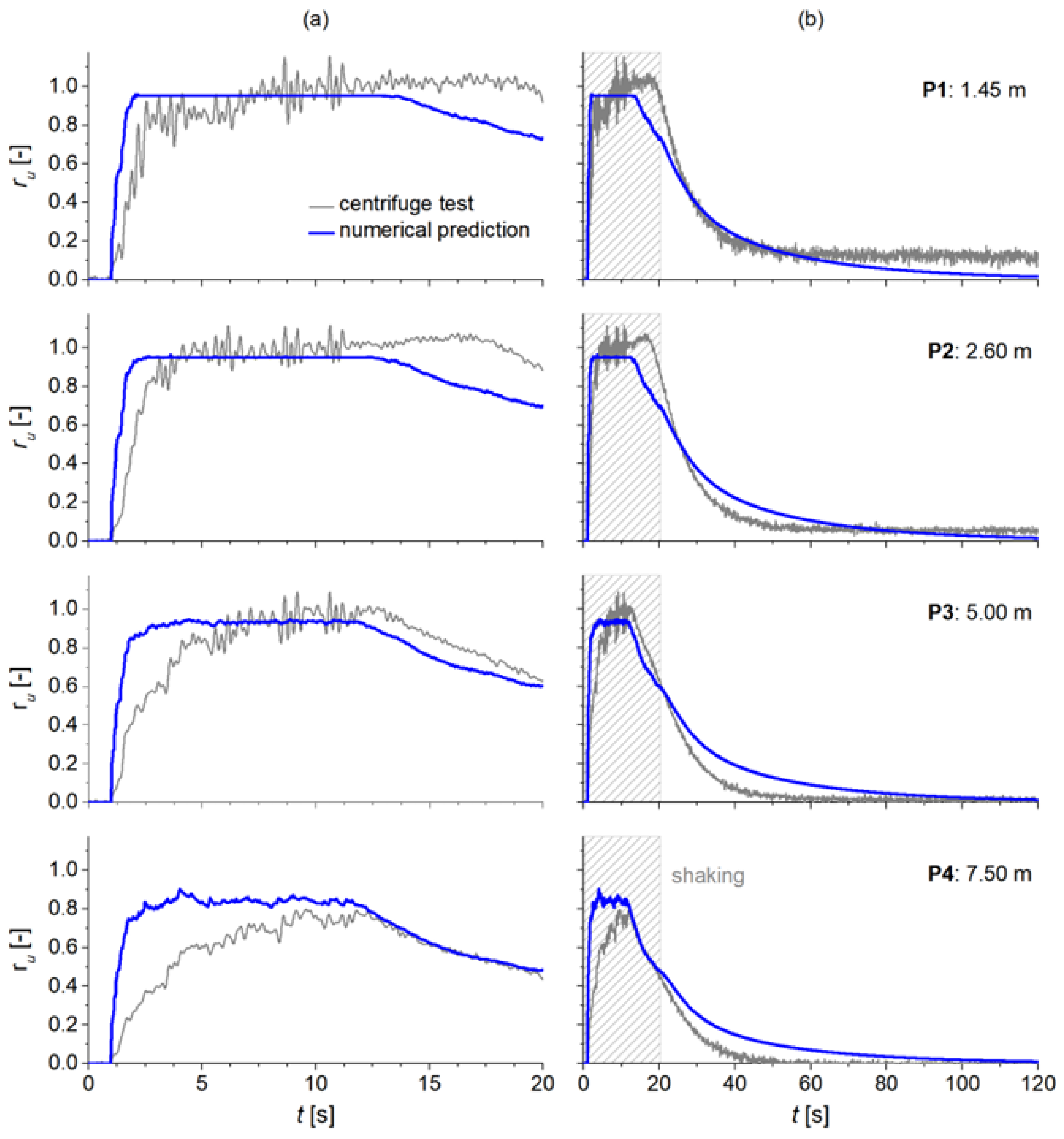
The results of the simulation, shown in
Figure 17, successfully predicted the pore pressure response. At depths of 1.45 m (P1), 2.6 m (P2), and 5 m (P3), the soil was predicted to liquefy, reaching a pore pressure ratio of 0.95 after 2 seconds of shaking. The model also accurately predicted that liquefaction would not occur at the 7.5 m depth (P4). Both the simulation and test results showed the typical pattern of initial pore pressure build-up followed by dissipation from the bottom up. However, the simulation showed maximum pore pressures occurring earlier at greater depths than in the actual test, possibly due to the model assuming a uniform density. The simulation also showed dissipation starting simultaneously at all depths, whereas the test results showed a delay in dissipation closer to the surface.
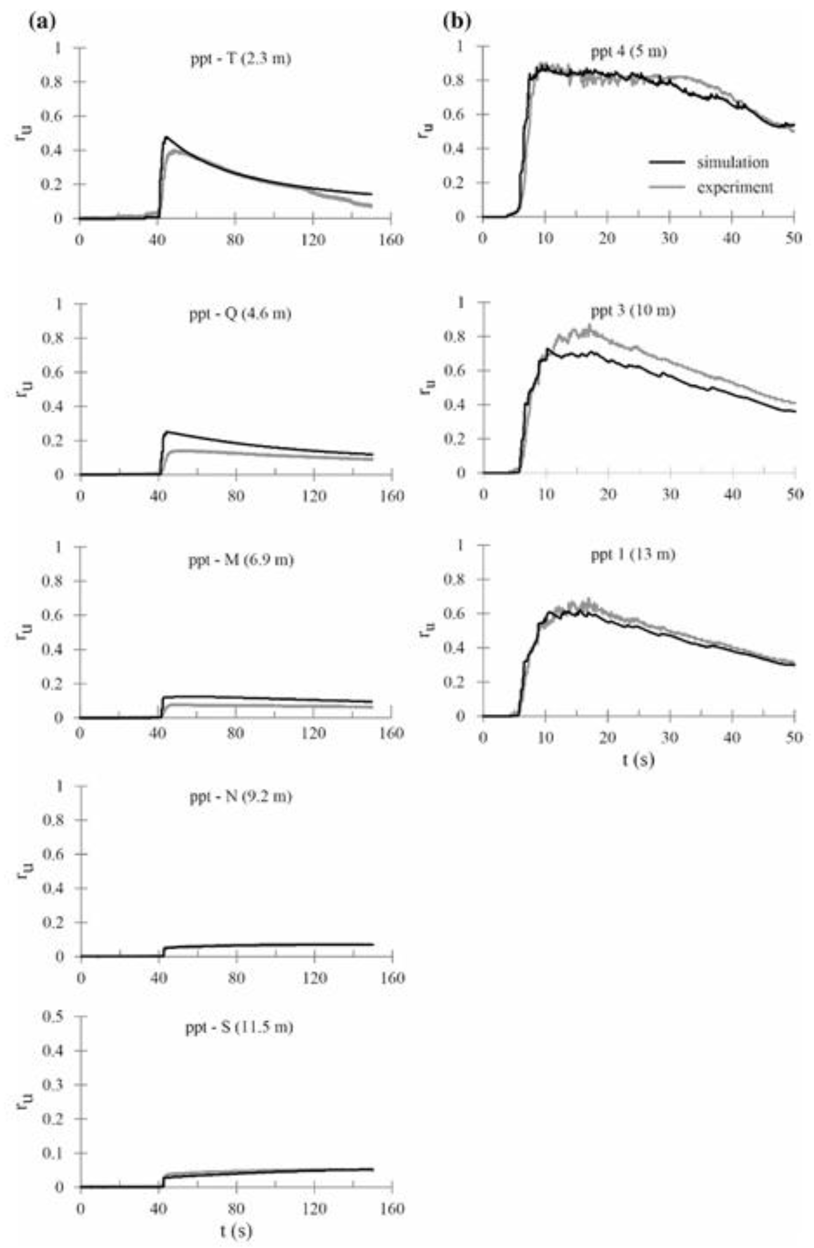
To demonstrate the capacity of the code to accurately predict the development of pore pressure even in conditions far from liquefaction, the simulations of the centrifuge tests on Ticino and Pieve di Cento sands as reported in [
75] are also presented in
Figure 18.
5.2. Detected Limitations
Several limitations or drawbacks can be detected in version 1 of the code:
The stick-slip model is validated against a few case studies and needs to be extended.
The numerical errors detected in the stick-slip scheme can be substantial.
The proposed method for liquefaction is not able to properly model the actual soil behaviour after the triggering of liquefaction.
The PWP model calibration on in-situ tests is based on the cyclic resistance curve analytically described by an exponential law, so the parameter CSRt tends to be zero.
The calibration of the PWP model for a specific relative density of the soil cannot be extended to a different relative density, but a new calibration of the model parameters is necessary even though the soil is the same.
The boundary conditions for dissipation and redistribution of excess pore water pressure are imposed only at the base of the soil profile.
Validation on soil models tested in centrifuge tests is limited to models made by a unique layer of sand, while layered configurations have not been considered yet.
6. Conclusions and Future Developments
The computer code SCOSSA version 1.0 has been demonstrated to be a valuable tool for the prediction of the seismic response of horizontally layered subsoil across the entire range of possible shear strains, from the smallest amplitudes up to liquefaction.
The model and the code were subjected to preliminary testing on an ideal soil profile, with the drainage conditions varying, and subsequently validated by comparing the predictions with the results of a centrifuge test and the seismic motions recorded at a well-documented array station.
The strong correspondence observed between numerical outcomes and experimental results underscores the reliability of the model incorporated within the code, despite the simplicity of the proposed approach.
In the short term, the code is undergoing a re-engineering process to enhance its management of input and output data. At the conclusion of this phase, a new version of the code will be released for free. It is anticipated that version 2.0 of the code will rectify or mitigate the aforementioned drawbacks.
In the long term, there is a proposal for the loosely coupled formulation to be integrated with the stick-slip model. This would facilitate the prediction of permanent deformation mechanisms.
Author Contributions
Conceptualization, A.C. and G.T,; methodology, A.C. and G.T.; software, A.C and G.T. ; validation, A.C. and G.T.; formal analysis, A.C. and G.T.; investigation, A.C. and G.T..; resources, A.C. and G.T..; data curation, A.C. and G.T.; writing—original draft preparation, A.C.; writing—review and editing, A.C. and G.T..; visualization, A.C. and G.T.; supervision, A.C. and G.T.; project administration, G.T..; funding acquisition, A.C. and G.T.. All authors have read and agreed to the published version of the manuscript.
Funding
We acknowledge financial support under the National Recovery and Resilience Plan (NRRP), Mission 4, Component 2, Investment 1.1, Call for tender No. 1409 published on 14.9.2022 by the Italian Ministry of University and Research (MUR), funded by the European Union – NextGenerationEU– Project Title "RI-SCOSSA 2.0 - Renovation and Improvement of Seismic COde for Stick-Slip Analyses" – CUP P20228HN9M Grant Assignment Decree No. 1385 adopted on 01-09-2023 by the Italian Ministry of Ministry of University and Research (MUR).
Data Availability Statement
The data presented in this study are available on request from the corresponding author.
Conflicts of Interest
The authors declare no conflicts of interest.
Abbreviations
The following abbreviations are used in this manuscript:
| PWP |
Pore Water Pressure |
| SCOSSA |
Seismic Computer cOde for Stick-Slip Analysis |
| CRR |
Cyclic Resistance Ratio |
| PreNoLin |
PREdiction of NOn-LINear soil behaviour |
| PGA |
Peak Ground Acceleration |
| MASW |
Multichannel Analysis of Surface Waves |
References
- NTC (2018) D.M. 17.01.2018 Aggiornamento delle Norme Tecniche per le Costruzioni.
- Rathje EM, Bray JD (2000) NONLINEAR COUPLED SEISMIC SLIDING ANALYSIS OF EARTH STRUCTURES. Geotech Geol Eng 1002–1014.
- Tropeano G, Chiaradonna A, d’Onofrio A, et al. (2016) An innovative computer code for 1D seismic response analysis including shear strength of soils. Geotechnique 66: 95–105. [CrossRef]
- Cubrinovski M, Rhodes A, Ntritsos N, et al. (2018) System response of liquefiable deposits. Soil Dyn Earthq Eng. [CrossRef]
- Dhakal R, Cubrinovski M (2025) Liquefaction response of reclaimed soils from effective stress analysis. Soils Found 65: 101677. [CrossRef]
- Hutabarat D, Bray JD (2021) Effective stress analysis of liquefiable sites to estimate the severity of sediment ejecta. J Geotech Geoenvironmental Eng 147: 4021024. [CrossRef]
- Tropeano G, Chiaradonna A, D’Onofrio A, et al. A Numerical Model for Non-Linear Coupled Analysis on Seismic Response of Liquefiable Soils. Comput Geotech. [CrossRef]
- Chiaradonna A, Tropeano G, d’Onofrio A, et al. (2018) Development of a simplified model for pore water pressure build-up induced by cyclic loading. Bull Earthq Eng. [CrossRef]
- Terzaghi K (1943) Theoretical Soil Mechanics.
- Chiaradonna A, Flora A, d’Onofrio A, et al. (2020) A pore water pressure model calibration based on in-situ test results. Soils Found 60: 327–341. [CrossRef]
- Chiaradonna A, Monaco P, Tropeano G (2024) Variability of the seismic response of a liquefiable soil with the fines content as estimated via dilatometer tests, 7th International Conference on Geotechnical and Geophysical Site Characterization, 1548–1554.
- Chiaradonna A, d’Onofrio A, Bilotta E (2019) Assessment of post-liquefaction consolidation settlement. Bull Earthq Eng 17. [CrossRef]
- Mele L, Chiaradonna A, Lirer S, et al. (2021) A robust empirical model to estimate earthquake-induced excess pore water pressure in saturated and non-saturated soils. Bull Earthq Eng 19: 3865–3893. [CrossRef]
- Chiaradonna A, Ntritsos N, Cubrinovski M (2022) CPT-based model calibration for effective stress analysis of layered soil deposits, Cone Penetration Testing 2022, CRC Press, 876–882.
- Chiaradonna A, Santisi D’Avila MP, Lenti L (2022) Seismic response of a 1D soil profile using two modeling approaches in effective stress condition, Proceedings of the International Conference on Natural Hazards and Infrastructure.
- Chiaradonna A, Tropeano G, d’Onofrio A, et al. (2018) Interpreting the deformation phenomena of a levee damaged during the 2012 Emilia earthquake. Soil Dyn Earthq Eng 1–10. [CrossRef]
- Chiaradonna A, Bilotta E, D’Onofrio A, et al. (2018) Geotechnical Earthquake Engineering and Soil Dynamics V GSP 293 394, Geesd V, 394–403.
- Ausilio E, Costanzo A, Silvestri F, et al. (2008) Prediction of seismic slope displacements by dynamic stick-slip analyses. AIP Conf Proc 1020: 475–484.
- Tropeano G, Ausilio E, Costanzo A (2011) Non-linear coupled approach for the evaluation of seismic slope displacements, V International Conference on Earthquake Geotechnical Engineering.
- Tropeano G, Chiaradonna A, D’Onofrio A, et al. (2016) An innovative computer code for 1D seismic response analysis including shear strength of soils. Géotechnique 66: 95–105. [CrossRef]
- Régnier J, Bonilla LF, Bard PY, et al. (2016) International benchmark on numerical simulations for 1D, nonlinear site response (Prenolin): Verification phase based on canonical cases. Bull Seismol Soc Am 106: 2112–2135. [CrossRef]
- Régnier J, Bonilla L, Bard P, et al. (2018) PRENOLIN: International Benchmark on 1D Nonlinear Site-Response Analysis—Validation Phase Exercise. Bull Seismol Soc Am. [CrossRef]
- Tropeano G, Evangelista L, Silvestri F, et al. (2016) 1D seismic response analysis of soil-building systems including failure shear mechanisms. Procedia Eng 158: 308–313. [CrossRef]
- Chiaradonna A, Tropeano G, d’Onofrio A, et al. (2016) A Simplified Method for Pore Pressure Buildup Prediction: From Laboratory Cyclic Tests to the 1D Soil Response Analysis in Effective Stress Conditions. Procedia Eng 158: 302–307. [CrossRef]
- Kuhlemeyer RL, Lysmer J (1973) Finite element method accuracy for wave propagation problems. J Soil Mech Found Div 99: 421–427. [CrossRef]
- Rayleigh JWS, Lindsay RB The theory of sound.
- Hashash YMA, Park D (2002) Viscous damping formulation and high frequency motion propagation in non-linear site response analysis. Soil Dyn Earthq Eng 22: 611–624. [CrossRef]
- Newmark NM (1959) A method of computation for structural dynamics. J Eng Mech Div 85: 67–94.
- Matasovic N, Vucetic M (1993) Cyclic Characterization of Liquefiable sands. J Geotech Eng 119: 1805–1822. [CrossRef]
- Phillips C, Hashash YMA (2009) Damping formulation for nonlinear 1D site response analyses. Soil Dyn Earthq Eng 29: 1143–1158. [CrossRef]
- Kramer SL (1996) Geotechnical earthquake engineering, Pearson Education India.
- Kramer SL, Stewart JP (2024) Geotechnical earthquake engineering, CRC Press.
- Chiaradonna A (2022) Defining the Boundary Conditions for Seismic Response Analysis—A Practical Review of Some Widely-Used Codes. Geosciences 12: 83. [CrossRef]
- Bardet JP, Ichii K, Lin CH (2000) EERA a Computer Program for E quivalent-linear E arthquake site Response Analyses of Layered Soil. Univ Calif 40.
- Kottke AR, Wang X, Rathje EM (2018) Strata Technical Manual.
- Hashash YMA, Musgrove MI, Harmon JA, et al. (2020) DEEPSOIL 7.0, user manual. Urbana, IL, Board Trust Univ Illinois Urbana-Champaign 1–170.
- Lu J, Elgamal A-WM, Yang Z (2006) Cyclic1D: a computer program for seismic ground response, Department of Structural Engineering, University of California, San Diego.
- GEO-SLOPE International Ltd. (2014) Dynamic Modeling With QUAKE/W. 1–173.
- Brinkgreve RBJ, Engin E, Swolfs WM (2016) PLAXIS 2D Reference Manual 2016. Plaxis 2016 454.
- Itasca Consulting Group (2016) Online Manual. FLAC Man.
- Itasca Consulting Group (2021) FLAC3D - Fast Lagrangian Analysis of Continua in 3 Dimensions. User’s Guide.
- Corporatio O (2014) No Title.
- Vucetic M, Dobry R (1991) Effect of soil plasticity on cyclic response. J Geotech Eng 117: 89–107. [CrossRef]
- Hashash Y, Phillips C, Groholski DR (2010) Recent advances in non-linear site response analysis.
- Matasovic N, Hashash YMA, National Academies of Sciences and Medicine E (2012) Practices and procedures for site-specific evaluations of earthquake ground motions.
- Aubry D, Modaressi A (1996) GEFDYN, Manuel scientifique. Ec Cent Paris.
- Dafalias YF, Manzari MT (2004) Simple plasticity sand model accounting for fabric change effects. J Eng Mech 130: 622–634. [CrossRef]
- Boulanger RW, Ziotopoulou K (2018) PM4Silt (Version 1): A silt plasticity model for earthquake engineering applications.
- Matasovic N (1993) Seismic response of composite horizontally-layered soil deposits, University of California, Los Angeles.
- Matasovic N, Ordonez GA (2011) DMOD 2000: A computer program for nonlinear seismic response analysis of horizontally layered soil deposits, earthfill dams and solid waste landfills. Lacey, WA GeoMotions, LLC.
- Moreno-Torres O, Hashash YMA, Olson SM (2010) A simplified coupled soil-pore water pressure generation for use in site response analysis, GeoFlorida 2010: Advanced in Analysis, Modeling & Design, 3080–3089.
- Bažant ZP, Krizek RJ (1976) Endochronic constitutive law for liquefaction of sand. J Eng Mech Div 102: 225–238. [CrossRef]
- Valanis KC (1971) A theory of viscoplasticity without a yield surface. Arch Mech Stos 23: 515–553.
- Finn WDL, Bhatia SK (1981) Prediction of seismic porewater pressures. Nucl Physics, Sect A 201–206.
- Ivšić T (2006) A model for presentation of seismic pore water pressures. Soil Dyn Earthq Eng 26: 191–199. [CrossRef]
- Park D, Ahn J (2013) Accumulated stress based model for prediction of residual pore pressure. 18th Int Conf Soil Mech Geotech Eng - Challenges Innov sin Geotech 1563–1566.
- Park T, Park D, Ahn J-K (2015) Pore pressure model based on accumulated stress. Bull Earthq Eng 13: 1913–1926. [CrossRef]
- Seed HB (1975) Representation of irregular stress time histories by equivalent uniform stress series in liquefaction analyses, College of Engineering, University of California.
- Annaki M, Lee KL (1977) Equivalent uniform cycle concept for soil dynamics. J Geotech Eng Div 103: 549–564. [CrossRef]
- Liu AH, Stewart JP, Abrahamson NA, et al. (2001) Equivalent number of uniform stress cycles for soil liquefaction analysis. J Geotech Geoenvironmental Eng 127: 1017–1026. [CrossRef]
- Green RA, Terri GA (2005) Number of equivalent cycles concept for liquefaction evaluations—Revisited. J Geotech Geoenvironmental Eng 131: 477–488. [CrossRef]
- Seed HB, Martin PP, Lysmer J (1976) Pore-water pressure changes during soil liquefaction. J Geotech Eng Div 102: 323–346. [CrossRef]
- Boulanger RW, Idriss IM (2014) CPT and SPT based liquefaction triggering procedures. Cent Geotech Model 134.
- Mandokhail SJ, Park D, Yoo J-K (2017) Development of normalized liquefaction resistance curve for clean sands. Bull Earthq Eng 15: 907–929. [CrossRef]
- Park T, Park D, Ahn JK (2015) Pore pressure model based on accumulated stress. Bull Earthq Eng 13: 1913–1926. [CrossRef]
- Ntritsos N, Cubrinovski M (2020) A CPT-based effective stress analysis procedure for liquefaction assessment. Soil Dyn Earthq Eng 131: 106063. [CrossRef]
- Cubrinovski M, Ishihara K (1998) Modelling of sand behaviour based on state concept. Soils Found 38: 115–127. [CrossRef]
- Cubrinovski M, Ishihara K (1998) State concept and modified elastoplasticity for sand modelling. Soils Found 38: 213–225. [CrossRef]
- Chiaradonna A, Tropeano G, Monaco P (2023) Numerical quantification of the dependency of the seismic site response on the DMT-based cyclic strength of sands, Proceedings 10th NUMGE 2023 10th European Conference on Numerical Methods in Geotechnical Engineering.
- Chiaradonna A, Monaco P (2025) DMT-based liquefaction triggering procedure accounting for the fines content effect. Soil Dyn Earthq Eng 199: 109668. [CrossRef]
- de Cristofaro M, Asadi MS, Chiaradonna A, et al. (2024) Modeling the Excess Porewater Pressure Buildup in Pyroclastic Soils Subjected to Cyclic Loading. J Geotech Geoenvironmental Eng 150: 6024007. [CrossRef]
- Khalil C, Régnier J, Lopez-caballero F (2022) LICORNE a benchmark on numerical method for non-linear site response analysis involving pore water pressure, 3rd EUROPEAN CONFERENCE ON EARTHQUAKE ENGINEERING & SEISMOLOGY.
- Chiaradonna A, Tropeano G, d’Onofrio A, et al. (2019) Interpreting the deformation phenomena of a levee damaged during the 2012 Emilia earthquake. Soil Dyn Earthq Eng 124: 389–398. [CrossRef]
- Chiaradonna A, Reder A (2020) Influence of initial conditions on the liquefaction strength of an earth structure. Bull Eng Geol Environ 79. [CrossRef]
- Mele L, Chiaradonna A, Lirer S, et al. (2020) A robust empirical model to estimate earthquake-induced excess pore water pressure in saturated and non-saturated soils. Bull Earthq Eng. [CrossRef]
- Chiaradonna A, Lirer S, Flora A (2020) A liquefaction potential integral index based on pore pressure build-up. Eng Geol 272: 105620. [CrossRef]
- Caputo P, Chiaradonna A, Di Ludovico M, et al. (2019) Soil liquefaction and induced damage to structures: A case study from the 2012 Emilia earthquake, Earthquake Geotechnical Engineering for Protection and Development of Environment and Constructions, CRC Press, 1596–1603.
- Merli A, Dezi F, Tropeano G, et al. (2019) Site response analysis in effective stress of a coastal area in the North-Western Adriatic region (Italy), Earthquake Geotechnical Engineering for Protection and Development of Environment and Constructions, CRC Press, 3893–3900.
- Abdoun T, Kokkali P, Zeghal M Physical Modeling of Soil Liquefaction: Repeatability of Centrifuge Experimentation at RPI. ASTM.
- Manzari MT, El Ghoraiby MA, Kutter BL, et al. (2019) Modeling the cyclic response of sands for liquefaction analysis. Earthq Geotech Eng Prot Dev Environ Constr Proc 7th Int Conf Earthq Geotech Eng 2019 385–396.
- Kokkali P, Abdoun T, Zeghal M (2017) Physical modeling of soil liquefaction: Overview of LEAP production test 1 at Rensselaer Polytechnic Institute. Soil Dyn Earthq Eng 1–21. [CrossRef]
- Ghofrani A, Arduino P (2017) Prediction of LEAP centrifuge test results using a pressure-dependent bounding surface constitutive model. Soil Dyn Earthq Eng 1–13. [CrossRef]
- Ramirez J, Barrero AR, Chen L, et al. (2018) Site Response in a Layered Liquefiable Deposit: Evaluation of Different Numerical Tools and Methodologies with Centrifuge Experimental Results. J Geotech Geoenvironmental Eng 144: 04018073. [CrossRef]
- Ziotopoulou K (2015) Seismic response of liquefiable sloping ground: Class A and C numerical predictions of centrifuge model responses. Soil Dyn Earthq Eng 1–14. [CrossRef]
- Cubrinovski M, Ishihara K, Tanizawa F (1996) Numerical simulation of the Kobe Port Island liquefaction. Proc 11th World Conf … 8.
- Zeghal, M., Elgamal, A., Parra E (1996) Analysis of site liquifaction using downhole array seismic records. Elev World Conf Earthq Eng.
- Cubrinovski M, Ishihara K, Furukawazono K (2000) Analysis of Two Case Histories on Liquefaction of Reclaimed Deposits. Proc 12th World Conf … 1–8.
- Ishihara K, Cubrinovski M (2005) Characteristics of ground motion in liquefied deposits during earthquakes. J Earthq Eng 9: 1–15. [CrossRef]
- Ziotopoulou K, Boulanger RW, Kramer SL (2012) Site Response Analysis of Liquefying Sites, GeoCongress 2012, 1799–1808.
- Shibata T, Oka F, Ozawa Y (1996) Characteristics of ground deformation due to liquefaction. Spec Issue Soils Found 65–79. [CrossRef]
- Carlton B (2014) An improved description of the seismic response of sites with high plasticity soils, organic clays, and deep soft soil deposits, University of California, Berkeley.
- Paul SM, Chiaradonna A, Chiaro G (2024) Numerical modelling of the dynamic behavior of gravel-rubber mixtures and their efficiency as liquefaction countermeasures. Japanese Geotech Soc Spec Publ 10: 2414–2419. [CrossRef]
- Dobry R, W.G. P, Dyvik R, et al. (1985) Pore pressure model for cyclic straining of sand.
- Vucetic M, Dobry R (1988) Cyclic triaxial strain-controlled testing of liquefiable sands.
- Chiaradonna A, Mohammadi R (2024) A milestone for liquefaction modelling: the instrumented vertical array of Port Island after the 1995 Kobe earthquake. Japanese Geotech Soc Spec Publ 10: 178–183. [CrossRef]
- Chiaradonna A, Mohammadi R, Monaco P (2024) Simulation of the Seismic Response of a Man-Made Well-Graded Gravel as Recorded by a Vertical Instrumented Array, Geo-Congress 2024, 132–140.
- Boulanger RW, Ziotopoulou K (2017) PM4Sand (version 3.1): A sand plasticity model for earthquake engineering applications. Rep. No, UCD/CGM-17/01. Davis, CA: Center for Geotechnical Modelling, Department of Civil and Environmental Engineering, University of California, Davis, CA, 108 pp.
- Ziotopoulou A (2010) Evaluating model uncertainty against strong motion records at liquefiable sites, Masters Abstracts International.
- Arulanandan K, Manzari M, Zeng X, et al. (1995) Significance of the VELACS project to the solution of boundary value problems in geotechnical engineering.
- Arulmoli K, Muraleetharan KK (1992) VELACS Laboratory testing program Soil data report.
|
Disclaimer/Publisher’s Note: The statements, opinions and data contained in all publications are solely those of the individual author(s) and contributor(s) and not of MDPI and/or the editor(s). MDPI and/or the editor(s) disclaim responsibility for any injury to people or property resulting from any ideas, methods, instructions or products referred to in the content. |
© 2025 by the authors. Licensee MDPI, Basel, Switzerland. This article is an open access article distributed under the terms and conditions of the Creative Commons Attribution (CC BY) license (http://creativecommons.org/licenses/by/4.0/).