Affordability in Hours: A Time-Indexed Minimum Wage and an Essential Hours Credit

Alec Pow; Lora Stonden

doi:10.20944/preprints202510.1728.v1

Submitted:

13 October 2025

Posted:

22 October 2025

You are already at the latest version

Abstract

We measure Monthly Survival Hours (MSH, or Essential Hours), the paid work time required to buy a fixed essentials basket, revealing a sharp affordability crisis: D3 renter hours spiked 50% from 117.4 hours (2019) to 175.7 hours (2022), with 2025 levels at 157.7 hours. We test two implementable policies: a Time-Indexed Minimum Wage (TIMW) that sets the wage floor by rule wmin,t = Ct/Htarget to cap essentials at 120 hours/month, and an Essential Hours Tax Credit (EHTC) that refunds gaps below 100 hours/month for low-wage cohorts via monthly advances. Using CPI components and CPS/OEWS wages across six metros, we show how TIMW stabilizes MSH near target while EHTC backstops D1–D3 renters during shocks, delivering a dual-key hours guarantee without price controls. Case studies for Phoenix, NYC, and Houston illustrate both ends of the metro spread. Preferred citation: Pow, A., & Stonden, L. (2025). Affordability in Hours: A Time-Indexed Minimum Wage and an Essential Hours Credit. SocArXiv. https://doi.org/10.31235/osf.io/ This Preprints.org posting is a discoverability mirror. Please cite the SocArXiv DOI above.

Keywords:

affordability

;

monthly survival hours (MSH)

;

minimum wage indexation (TIMW)

;

refundable tax credit (EHTC)

;

CPI

;

labor economics

Subject:

Business, Economics and Management - Finance

1. Introduction

Project: Affordability in Hours: A Time-Indexed Minimum Wage and an Essential Hours Credit · 2025

Problem → Thesis → Contributions

1.1. Problem

Households experience affordability through time, not just prices: when essentials' cost rises faster than wages, required hours to meet basic needs increase, especially for renters and low-wage work. The post-COVID inflation crisis (2020-2022) quickly accelerated this trend, with MSH for D3 renters spiking from 117.4 hours (2019) to 175.7 hours (2022) as inflation outpaced wage growth. We formalize this as MSH and measure it with official price and wage statistics. [1,2]

1.2. Thesis

A dual-key system using TIMW to anchor affordability for all workers and EHTC to backstop the lowest deciles can hold MSH near explicit targets while respecting regional variation and employer adjustment frictions documented in the minimum-wage literature. [6,7]

1.3. Contributions

(i) A transparent hours-based dashboard for essentials; (ii) policy rules expressed directly in hours, with glide caps and guardrails; (iii) implementable delivery rails using refundable credit infrastructure demonstrated in 2021 monthly advances. [5]

1.4. Research Questions & Hypotheses

RQ1: How did MSH evolve from 2000 to 2025 by decile, occupation, and metro? H1: Differences are driven by housing and energy shares interacting with wage growth patterns across three distinct economic eras (pre-GFC, GFC-to-COVID, pandemic/inflation).
RQ2: Can TIMW (semi-annual) maintain H_target = 120 hours/month under a ≤5% glide cap without inducing volatility? H2: Region bands and small-firm phase-ins stabilize adjustments.
RQ3: Can EHTC close gaps below H_threshold = 100 hours/month for D1–D3 without large pass-through or targeting leakage? H3: ZIP-level staggered pilots detect impacts on arrears and credit costs.

2. Background & Related Work

Project: Affordability in Hours: A Time-Indexed Minimum Wage and an Essential Hours Credit · 2025

2.1. Background Map (Taxonomy)

A. Inflation & real wages

CPI essentials sub-indexes (food at home, electricity, telephone/internet, rent/OER). [1,8]
Wage deciles (CPS) and occupations (OEWS). [2,3]

B. Housing split (renter vs owner)

Rent vs Owner’s Equivalent Rent (OER) handling and the Renter’s Surcharge construct. [1]

C. Checkout uplift (fees & tips)

Sticker-to-receipt gap (fees, tips, delivery). Sensitivity ranges; reporting templates. [1]

D. Mobility (car vs transit)

Energy/transport: gasoline vs public transit assumption by cohort; electricity as an essentials input. [4]

E. Equity splits

Deciles (D1–D10), eight occupations, six metros; decomposition by price vs wage. [2,3]

2.2. Positioning This Study

This review situates Monthly Survival Hours (MSH) among (i) inflation and index-number methodologies, (ii) distributional & household-specific price measurement, (iii) wage-floor and income-support literatures, and (iv) consumer-protection work on price transparency. Our approach contributes a time-denominated affordability metric that is auditable (CPI-based), distributional (deciles/occupations), and policy-coupled (TIMW/EHTC).

Index numbers Distributional inflation Minimum wage Tax credits (EITC/CTC) All-in pricing / fees Housing measurement (OER/Rent) Energy affordability Digital inclusion (telecom)

2.3. Inflation Measurement & Index-Number Theory

We adopt a Laspeyres-style aggregation with fixed 2019 weights for transparency and comparability (Ch. 3–4). The CPI handbooks provide item definitions, sampling, and adjustment procedures; superlative indices (e.g., Fisher, Törnqvist) reduce substitution bias at the cost of simplicity. Because our objective is distributional affordability rather than a COLI per se, fixed weights are defensible and sensitivity bands (±10%) guard against composition risk [1,2].

CPI documentation: classification, hedonic adjustments, seasonal factors [1,2].
Weights choice: Laspeyres vs superlatives; we report robustness rather than re-weight monthly.

2.4. Distributional & Household-Specific Inflation

Households experience different inflation paths due to heterogeneous baskets and geography. Prior work constructs household-level or group-specific price indices and documents inflation inequality. Our contribution focuses on essentials only (housing, food-at-home, electricity, telecom, transport) and expresses the burden in hours, not dollars, which makes policy thresholds clearer. We localize via metro CPI where available and otherwise use regional proxies with full disclosure [1].

Group-specific or distributional indices highlight heterogeneity by income or demographics (selected syntheses; add journal citations in numbered during final pass).
Our Renter’s Surcharge aligns with literature separating renter/owner dynamics via Rent vs OER treatment.

2.5. Housing Measurement: Rent vs. Owners’ Equivalent Rent (OER)

Housing dominates essentials. CPI measures owner costs via OER and renter costs via observed rent, with known dynamics and lags. We mirror this: renter and owner baskets are identical except for the housing component, enabling a tenure gap in hours. Limitations and motivations are documented in CPI references; we treat OER as the accepted proxy and report the renter–owner hours gap as a descriptive equity statistic [1,2].

2.6. Wage Floors & Labor-Market Effects

A large empirical literature studies minimum-wage impacts on employment and earnings. Recent credible designs (border discontinuities, synthetic controls, modern DiD) find modest average employment effects and significant earnings gains at the bottom, with heterogeneity by sector and place. We build on these by tying the wage floor to an essentials basket (TIMW), adding glide caps and phase-ins to mediate adjustment costs [3,4,5].

Evidence reviews & quasi-experimental studies underpin our guardrails and cadence choices.
Our back-tests/forward-tests (Ch. 5) align with this literature’s emphasis on transparent counterfactuals.

2.7. Refundable Tax Credits & Monthly Advances

Refundable credits (EITC/CTC) are well-studied; they raise after-tax incomes, reduce poverty, and can be delivered in advances using existing administrative rails. The Essential Hours Tax Credit (EHTC) is a targeted variant that pegs benefits to the hours gap above a threshold, with reconciliation at filing and audit mechanisms similar to EITC practices [6,7].

Design elements (eligibility, take-up, reconciliation) follow tax-credit playbooks; we contribute a novel hours-based benefit rule.

2.8. Consumer Fees, All-In Pricing & Effective Costs

Hidden fees and default tips can widen sticker→receipt gaps, obscuring effective prices. Regulatory guidance on “junk fees” motivates our checkout uplift parameter and all-in pricing complement to TIMW/EHTC. Penalties can be recycled as offsets in budget scoring (Ch. 5) [8].

2.9. Energy & Digital Inclusion in Essentials

Electricity and telecom are essential modern services. CPI electricity indexes track service prices; EIA’s ¢/kWh series serve as diagnostics. For telecom, CPI tracks “Telephone services” and “Internet/electronic information providers”; we combine them 50:50 absent stronger evidence for bundle shares (Ch. 3–4) [9,1].

2.10. Gaps Our Study Addresses

From prices → time

We translate CPI prices and wages into hours, a salient currency for households and policymakers. This reframing yields auditable thresholds and guardrails.

From measurement → action

We bind a descriptive metric (MSH) to implementable levers (TIMW/EHTC), closing the loop between diagnosis and policy.

From averages → distribution

We report deciles, occupations, and tenure splits—surfacing equity impacts that aggregate inflation statistics can mask.

From national → local

We localize with metro CPI, disclosing proxies; metro comparisons and renter–owner gaps turn national narratives into actionable local dashboards.

3. Data Dictionary & Cohorts

Project: Affordability in Hours: A Time-Indexed Minimum Wage and an Essential Hours Credit · 2025

3.1. Overview & Sourcing Principles

This chapter specifies all price and wage series, cohort definitions, geographic cuts, and reproducibility rules used to compute Monthly Survival Hours (MSH). Price indices are sourced from the U.S. Bureau of Labor Statistics (BLS) Consumer Price Index (CPI) program; wages come from BLS CPS/OEWS publications; energy prices may be cross-validated with EIA for diagnostics; public transport price proxies may use CPI subcomponents or FTA/BTS resources where appropriate [1,2,3,4,5,6]. All datasets are public and version-pinned at download time for replicability [9].

Frequency: monthly where possible. Units: hours/month for results; $/hour for wages; CPI rebased to 2019=1. Period: 2000–2025 (indices rebased to 2019=1; use latest available month).

3.2. Series Inventory (Data Dictionary)

Table 3.1. Core price and wage series.

Domain	Concept	Source	Freq.	Units	Series ID/Code	Endpoint/URL	Notes
Prices (CPI)	Rent of primary residence (renter basket)	BLS CPI	Mo.	Index (2019=1 after rebasing)	CUUR0000SEHA	https://www.bls.gov/cpi/	Core housing price for renter cohorts [1,2]
Prices (CPI)	Owners’ equivalent rent (owner basket)	BLS CPI	Mo.	Index (2019=1)	CUUR0000SEHC	https://www.bls.gov/cpi/	Used to proxy owner housing cost [1]
Prices (CPI)	Food at home	BLS CPI	Mo.	Index (2019=1)	CUUR0000SAF11	https://www.bls.gov/cpi/	Groceries only (excludes food-away-from-home) [2]
Prices (CPI)	Electricity (residential)	BLS CPI	Mo.	Index (2019=1)	CUUR0000SEHF01	https://www.bls.gov/cpi/	Can cross-check with EIA price per kWh trends [5]
Prices (CPI)	Internet & electronic information providers	BLS CPI	Mo.	Index (2019=1)	CUUR0000SEEE03	https://www.bls.gov/cpi/	Use with Telephone services for bundled "Phone/Internet" [2]
Prices (CPI)	Telephone services	BLS CPI	Mo.	Index (2019=1)	CUUR0000SEED	https://www.bls.gov/cpi/	Combine with Internet index to proxy a basic plan [2]
Prices (CPI)	Gasoline (all types)	BLS CPI	Mo.	Index (2019=1)	CUUR0000SETB01	https://www.bls.gov/cpi/	Choose as transport option for car cohorts; alt: Public transport [2]
Prices (CPI)	Public transportation	BLS CPI	Mo.	Index (2019=1)	CUUR0000SETG	https://www.bls.gov/cpi/	Choose as transport option for transit cohorts [2,6]
Wages (CPS)	Hourly wage by decile (D1…D10)	BLS CPS/ASEC	Mo./ Ann.	$ per hour	CPS microdata	https://www.bls.gov/cps/	Construct deciles from CPS microdata or use published percentiles [3]
Wages (OEWS)	Occupation median wage — Cashier (SOC 41-2011)	BLS OEWS	Ann.	$ per hour	SOC:41-2011	https://www.bls.gov/oes/	Map to occupation cohorts; harmonize to monthly timeline [4]
Wages (OEWS)	Occupation median wage — Nurse (SOC 29-1141/1161)	BLS OEWS	Ann.	$ per hour	SOC:29-1141/1161	https://www.bls.gov/oes/	Pick RN or combined nursing occupations per study design [4]
Wages (OEWS)	Occupation median wage — Teacher (SOC 25-2021 etc.)	BLS OEWS	Ann.	$ per hour	SOC:25-xxxx	https://www.bls.gov/oes/	Use hourly equivalents where available [4]
Wages (OEWS)	Occupation median wage — Software engineer (SOC 15-1252)	BLS OEWS	Ann.	$ per hour	SOC:15-1252	https://www.bls.gov/oes/	Rep for upper-decile cohorts [4]
Wages (OEWS)	Occupation median wage — Truck driver (SOC 53-3032)	BLS OEWS	Ann.	$ per hour	SOC:53-3032	https://www.bls.gov/oes/	Non-metro sensitivity possible [4]
Wages (OEWS)	Occupation median wage — Retail sales (SOC 41-2031)	BLS OEWS	Ann.	$ per hour	SOC:41-2031	https://www.bls.gov/oes/	Lower-wage cohort representation [4]
Wages (OEWS)	Occupation median wage — Electrician (SOC 47-2111)	BLS OEWS	Ann.	$ per hour	SOC:47-2111	https://www.bls.gov/oes/	Skilled trade cohort [4]
Wages (OEWS)	Occupation median wage — Caregiver/Home health aide (SOC 31-1120)	BLS OEWS	Ann.	$ per hour	SOC:31-1120	https://www.bls.gov/oes/	Care economy cohort [4]
Geography	Regional/Metro CPI (where available)	BLS CPI	Mo.	Index (2019=1)	CUURA101SEHA, CUURA311SEHA, CUURA169SEHA, CUURA264SEHA, CUURA380SEHA, CUURA120SEHA	https://www.bls.gov/regions/cpi/	NYC, LA, Chicago, Houston, Phoenix, Atlanta metro indices [2]. Cite BLS area code file for metro codes
Diagnostics	Residential electricity price (¢/kWh)	EIA EPM	Mo.	¢/kWh	table_5_03 (national), epmt_5_6_a (by state)	https://www.eia.gov/electricity/monthly/	For chart notes only; CPI remains canonical in results [5]. EIA Electric Power Monthly
Diagnostics	Gasoline price (weekly)	EIA	Wkly.	$/gallon	EMM_EPMR_PTE_NUS_DPG	https://www.eia.gov/petroleum/gasdiesel/	Weekly gasoline price series; can cite FRED GASREGW mirror [7]
Diagnostics	Transit fare documentation	FTA/BTS	Var.	—	NTD fare data	https://www.transit.dot.gov/	Background on fare methodologies [6]. If computing "avg fare per trip," note BTS/NTD methodology uses unlinked passenger trips

Notes: All price indices are rebased to 2019=1 prior to use. Wages harmonized to monthly by linear interpolation or step-hold; see §2.4.

Data contracts (CSV schemas)

3.3. Cohorts & Geography

Table 3.2. Cohorts (distributional & occupational).

Group	Members	Definition/Mapping	Notes
Wage deciles	D1…D10	Percentiles of the hourly wage distribution from CPS (monthly or annual micro), converted to deciles	Construct via weighted percentiles; impute missing months with monotone interpolation [3]
Occupations	cashier, nurse, teacher, software engineer, truck driver, retail sales, electrician, caregiver	Map to OEWS SOC codes (see Table 2.1) and use median hourly wage per year; align to monthly timeline by step-hold	Occupation cohorts show heterogeneity beyond deciles [4]
Tenure	renter, owner	Identical baskets except housing: renters use “Rent of primary residence”; owners use “OER”	Enables Renter’s Surcharge analysis
Metros	NYC, Los Angeles, Chicago, Houston, Phoenix, Atlanta	Use metro CPI where available; otherwise regional CPI as proxy; include a national series	Document any substitutions explicitly [2]

Table 3.3. Cohort–basket mapping rules.

Cohort	Housing index	Transport option	Telecom bundle	Notes
D1–D3 (lower-wage)	Rent (renter) / OER (owner)	Gasoline (headline); transit only in robustness	Telephone + Internet (weighted mean)	Document choice of transport per metro; keep fixed within a given run
D5 (median)	Rent / OER	Gasoline	Telephone + Internet	Used in headline figures
D10 (upper-wage)	OER (owner) or Rent (if explicitly renter)	Gasoline	Telephone + Internet	Comparison baseline for equity gaps
Occupations (all)	As per tenure flag	Choose per occupation context (e.g., transit for urban teacher)	Telephone + Internet	State choices in figure notes
Transport must be consistently chosen within a figure/table. Sensitivity runs may switch between gasoline and public transport; report both when used.

3.4. Protocols: Frequency, Rebasing, Missingness, Version Pinning

Frequency & alignment

CPI series are monthly; wages may be monthly (CPS) or annual (OEWS). Align all series to a monthly grid. For OEWS annual medians, use step-hold (carry the latest observed value forward) unless a simple linear interpolation is explicitly tested in sensitivity [3,4].

Rebasing

Rebase each CPI component to 2019-01 = 1.000: p'_{i,t} = p_{i,t} / p_{i,2019-01}. Maintain a metadata record of the base month and original units [1].

Missingness

For brief CPI gaps, use last observation carried forward (LOCF). For wage decile gaps (if computed annually), use linear interpolation constrained by observed percentiles. Document all imputations in metadata.json and flag imputed cells in CSVs (boolean column imputed).

Version pinning

For each dataset pull, store download date, endpoint URL, series IDs, and program version (if provided) in metadata.json. When citing datasets, include version/DOI where applicable and an access date per DataCite recommendations [9].

3.5. Reproducibility Checklist (to Be Mirrored In Repo)

List exact BLS series IDs for all CPI components; list SOC codes for all occupations.
Download CSVs from primary endpoints; save to /data/raw/ with YYYYMMDD in filename.
Create metadata.json capturing source, URL, access date, series IDs, units, and transformations.
Rebase CPI to 2019-01 = 1.000; align wages to monthly grid; export processed files to /data/processed/.
Build prices.csv, wages.csv, and geography.csv exactly as specified in the Data contracts.
Log any imputations with an imputed boolean column; keep a human-readable CHANGELOG.md.
Run a smoke test that recomputes headline MSH for one cohort and month; verify units and base.
Freeze a release: tag the repo, export figures to /figures/, and archive to Figshare/OSF with appropriate related identifiers.

3.6. Notes & Caveats

Choice of transport index: Core run uses gasoline; transit appears only in robustness.
Occupation wages: OEWS medians are annual; mapping to monthly introduces step artifacts—flag clearly in captions.
Metro coverage: Some metros may lack complete CPI subcomponents; substitute regional CPI and disclose.
Licensing: All sources are public; derived data and code will be released under CC BY 4.0 with proper attribution.

4. Basket Definition & Calibration

Project: Affordability in Hours: A Time-Indexed Minimum Wage and an Essential Hours Credit · 2025

4.1. Purpose & Principles

This chapter defines the fixed "survival" consumption basket used to compute Monthly Survival Hours (MSH), and documents calibration rules so results are reproducible and comparable across cohorts, metros, and time. Components are deliberately limited to essential, high-salience categories that dominate low- to middle-income budgets: housing, groceries (food at home), electricity, phone/internet, and basic transport [1,2]. We use official price indices from the Bureau of Labor Statistics (BLS) CPI program and hold physical quantities or baseline dollar weights constant at their 2019 levels to isolate pure price and wage effects over 2000–2025 [1].

4.2. Basket Specification (2019 Baseline)

Two equivalent calibration modes are supported: (A) **Dollar-weighted** (recommended for simplicity with CPI indexes) and (B) **Physical-quantity** (diagnostic). For all CPI components we rebase the index to 2019-01=1.000 and compute basket cost as a Laspeyres-style aggregation with fixed 2019 weights [1,3].

Table 4.1. Core basket components and 2019 baseline weights.

Component	Index used	Mode A — Baseline monthly weight (USD, 2019)	Mode B — Baseline quantity (diagnostic)	Notes
Housing	Rent of primary residence (renter) / Owners’ equivalent rent (owner)	$900 (renter); $900 (owner via OER)	1 housing unit (price proxied by CPI index)	Only component that differs by tenure; see Table 3.2 [1]
Food at home (groceries)	CPI: Food at home	$275	Fixed weekly grocery list (diagnostic)	Excludes food away from home to avoid service volatility [1,2]
Electricity (residential)	CPI: Electricity	$90	600–750 kWh	Quantity range reflects climate/geography; index remains canonical [4]
Phone & Internet	Composite of CPI: Telephone services & Internet/Electronic information providers	$85	1 basic mobile + 1 basic broadband plan	50:50 index weighting unless specified otherwise [1]
Transport (headline)	CPI: Gasoline (all types)	$150 (gasoline)	~45 gal gasoline	Headline series; transit alternative in Robustness [1,5]
Weights are intentionally conservative, national baselines for a single-adult household in 2019 (stylized). Replace with CES-derived shares if desired; results remain comparable so long as weights are fixed over time [2].

Table 4.2. — Tenure variants (only housing differs).

Variant	Housing index	Other components	Comment
Renter basket	CPI: Rent of primary residence	Food at home; Electricity; Phone/Internet; Transport	Enables estimation of the Renter’s Surcharge [1]
Owner basket	CPI: Owners’ equivalent rent (OER)	Food at home; Electricity; Phone/Internet; Transport	Owner housing proxied per CPI practice [1]

Why fixed 2019 weights?

Using a fixed-weight (Laspeyres-style) basket isolates price and wage dynamics without confounding from substitution or changing quantities—appropriate for a distributional affordability metric rather than a cost-of-living index with substitution effects [1,3].

4.3. Calibration Rules

Rebasing CPI components

For each CPI series, rebase to 2019-01=1.000: p'_{i,t} = p_{i,t} / p_{i,2019-01}. Store base dates and original units in metadata.json [1].

Composite indices

Phone/Internet: compute a simple average of the two CPI components unless a documented bundle share is provided: p'_{tel+net,t} = 0.5·p'_{tel,t} + 0.5·p'_{net,t} [1].
Transport: Core run uses gasoline; transit appears only in robustness [1,5].

Metro localization

Where metro CPI is available, replace national CPI with metro series for Housing and other components; otherwise use regional CPI as a proxy. Document substitutions in captions and metadata.json [1].

Resulting basket cost

With Mode A (dollar weights), monthly basket cost is C_t = Σ_i q_i · p'_{i,t}, where q_i are the 2019 USD weights from Table 3.1. The baseline basket total is $1,500/month (gasoline transport mode). With Mode B (physical quantities), convert quantities to dollars using CPI-implied price relatives before aggregation; Mode A is recommended for parsimony [1,3].

Robustness ranges

Report a ±10% quantity/weight sensitivity for each component and, for transport, a gasoline↔transit switch (alternative to headline gasoline series); summarize impacts on MSH in the Robustness chapter [2].

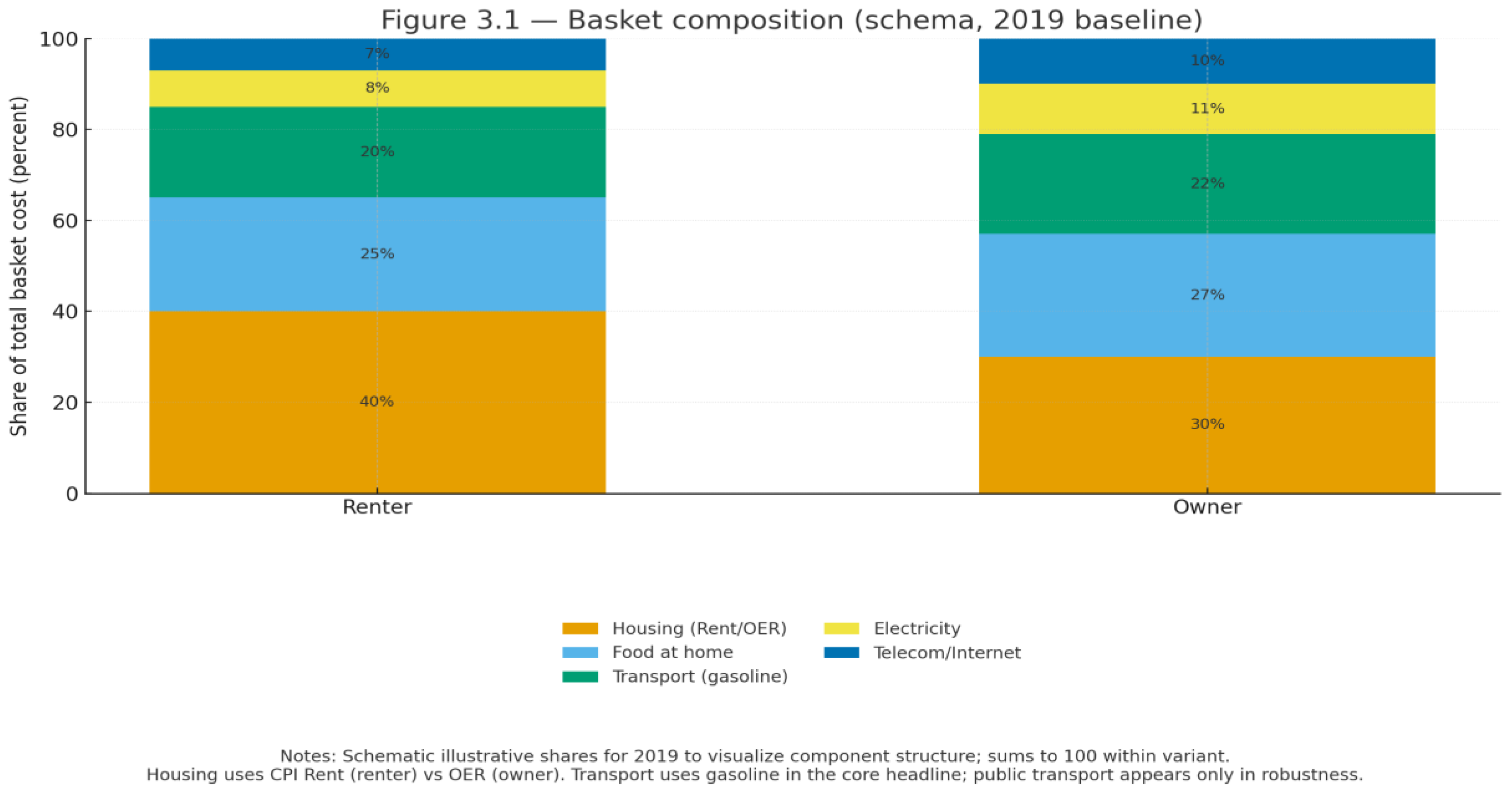
Figure 4.1. Basket composition (2019 shares). Share of total baseline basket cost by component for renter and owner variants. Housing uses CPI Rent (renter) vs OER (owner); other components are identical. Use Mode A (dollar weights) for this figure. Core run shows national shares; metro overlays optional. Data contract.

file: basket_shares.csv
columns:
  variant (renter|owner),
  component (housing|food_home|electricity|telecom|transport),
  share_2019 (0-1),
  share_2025 (0-1, optional for comparison)
notes:
  - shares sum to 1 within variant and year
  - telecom = composite of telephone & internet indices (50:50 unless specified)
  - transport = gasoline (headline); public_transport shown only in robustness

4.4. Cohort–Basket Mapping (Recap & Specifics)

Tenure: renter vs owner differs only in the housing index (Rent vs OER) [1].
Deciles & occupations: all use the same fixed basket; heterogeneity enters through wages w_{g,t} in MSH [3].

Core run uses gasoline; transit appears only in robustness.

Telecom bundle: 50:50 Telephone:Internet unless data justify an alternative share; document any change [1].

4.5. Operational Checklist

Populate prices.csv with CPI components rebased to 2019-01=1.000 (see Chapter 2 contracts) [1].
Set q_i to Table 3.1 Mode A values (or CES-derived values) and freeze in metadata.json [2].
Compute composite indices (telecom; chosen transport). Export basket_shares.csv for Figure 3.1.
Document metro substitutions and any weight sensitivities applied (±10%).

5. Methods & Measurement

Project: Affordability in Hours: A Time-Indexed Minimum Wage and an Essential Hours Credit · 2025

5.1. Measurement Framework

We express affordability as Monthly Survival Hours (MSH): the hours of work required to purchase a fixed essentials basket whose components and weights are frozen at a 2019 baseline to isolate price and wage dynamics over time [1,3]. Basket details appear in Chapter 3 and follow BLS CPI conventions for item classification and index treatment [1].

(1) (1) C_t = Σ_i q_i · p_{i,t}

Here q_i are fixed 2019 baseline weights (USD or quantities) and p_{i,t} are CPI item indexes rebased to 2019-01=1.000; we use a Laspeyres-style aggregation, appropriate for tracking the burden of essential expenditures without substitution adjustments [1,3].

(2) (2) H_{g,t} = C_t / w_{g,t}

w_{g,t} is the hourly wage for cohort g (wage decile or occupation), aligned to a monthly grid using CPS (for distribution) and OEWS (for occupations) per §4.4, with care to preserve level comparability across time and geographies [4,5].

5.2. Log-Change Decomposition

To attribute changes in hours to prices vs wages, we use a first-order log-change decomposition over 2019→t [3,4]:

(3) (3) Δ ln H_{g,t} ≈ Δ ln C_t − Δ ln w_{g,t}

Component contributions to Δ ln C_t are computed by cost shares using rebased CPI levels, enabling stacked displays (housing, food, electricity, telecom, transport) in Figure 2 [1].

5.3. Equity Splits & Distributional Metrics

(4) (4) RS_t = H^{renter}_{g,t} − H^{owner}_{g,t}

The Renter’s Surcharge (RS_t) contrasts renter vs owner baskets (Rent vs OER) for the same cohort to isolate tenure effects on essentials burden [1].

(5) (5) Gap_t = H_{D1..D3,t} − H_{D10,t}

The Decile Gap contrasts lower-wage deciles with the top decile to summarize distributional stress in hours terms [4].

(6) (6) ΔH^{metro}_{g,t} = H^{metro}_{g,t} − H^{national}_{g,t}

The Metro Differential benchmarks local hours against national levels using available metro/regional CPI to localize price dynamics [1].

5.4. Index Construction, Rebasing & Composites

Rebasing CPI components

For each component, rebase to 2019-01=1.000 using p'_{i,t} = p_{i,t} / p_{i,2019-01}; store base dates and original units in metadata.json to ensure reproducibility and auditability [1].

Telecom composite

Create a composite telecom index by a simple average of “Telephone services” and “Internet/electronic information providers” unless a documented bundle share is available: p'_{tel+net,t} = 0.5·p'_{tel,t} + 0.5·p'_{net,t} [1].

Transport choice

Core run uses gasoline; transit appears only in robustness [1,6].

Metro localization

Replace national CPI with metro CPI where available; otherwise use regional CPI proxies, disclosing substitutions in captions and metadata to retain transparency [1].

5.5. Wage Series Alignment (CPS & OEWS)

Deciles. Construct wage deciles D1…D10 from CPS microdata or use published percentiles; align to a monthly grid via weighted percentiles and constrained interpolation when needed, preserving level comparability [4].

Occupations. Use OEWS occupation medians (SOC codes in Chapter 2) and align annually via step-hold to months; where hourly rates are unavailable, convert from annual salary using standard hours assumptions and flag such conversions in metadata [5].

Quality controls. Track sample composition changes, top-coding, and breaks; report any methodology changes affecting time-consistency per BLS documentation to avoid spurious level shifts [4,5].

5.6. Sensitivity Design

Basket weights ±10%: perturb q_i and recompute H_{g,t}; report bands in robustness figures to assess composition risk [3].
Transport switch: gasoline ↔ public transport to assess mobility assumptions [1,6].
Wage measure: compare CPS deciles vs alternative measures (weekly earnings, within-occupation medians) [4,5].
Fee/tip uplift: apply bounds on checkout uplift Uplift_t and recompute Ĉ_t = C_t·(1+Uplift_t) for sensitivity figures [7].
Metro substitution: swap metro vs regional CPI where missing; document impacts to check geographic consistency [1].

5.7. Evaluation Designs for TIMW & EHTC

Pilot A (EHTC): a stepped-wedge (staggered ZIP rollout) difference-in-differences estimating the causal reduction in H_{g,t} for eligible cohorts, with ZIP and time fixed effects and clustered standard errors at the ZIP or county level to address serial correlation [8,9].

(7) (7) H_{z,t} = α_z + γ_t + β · (Treat_z × Post_t) + ε_{z,t}

We will use contemporary staggered DID estimators (e.g., Sun–Abraham, Callaway–Sant’Anna) to avoid negative-weight bias under heterogeneous treatment timing, and report event-study coefficients for pre-trend checks [9,10].

Pilot B (TIMW): back-test counterfactual wage floors using w_{min,t}=C_t/H_{target} for Phoenix/Atlanta and compare realized vs indexed paths; forward-simulate semi-annual updates with a ≤5% glide cap and report distributional effects on H_{g,t} [1,4].

5.8. Notation & Units

Table 5.1. Symbols and definitions.

Symbol	Definition	Units	Notes
q_i	Fixed 2019 basket weight (USD or quantity)	USD or qty/month	See Chapter 3
p_{i,t}	Price index for component i at time t (rebased)	Index (2019=1)	BLS CPI item series
C_t	Monthly basket cost	USD/month (relative)	Eq. (1)
w_{g,t}	Hourly wage for cohort g	USD/hour	CPS/OEWS
H_{g,t}	Monthly Survival Hours	hours/month	Eq. (2)
RS_t	Renter’s Surcharge	hours/month	Eq. (4)
Uplift_t	Sticker→receipt uplift (fees/tips)	fraction	0–1 bounds
Ĉ_t	Cost with uplift applied	USD/month (relative)	Ĉ_t=C_t·(1+Uplift_t)
w_{min,t}	Time-indexed minimum wage	USD/hour	=C_t/H_target

5.9. Algorithm (Pseudocode) to Compute MSH

// inputs: prices.csv, wages.csv, basket weights q_i, mapping rules, base month = 2019-01
// output: hours.csv with columns: date, cohort, hours

1. Load prices.csv; verify each component is rebased to 2019-01 = 1.000 [1].
2. Construct composite telecom index; select transport index per cohort and fix choice for the run [1,6].
3. Compute C_t = Σ_i q_i * p_{i,t} for each date t using Mode A weights (Chapter 3) [1,3].
4. Load wages.csv; align CPS deciles monthly; align OEWS occupation medians by step-hold [4,5].
5. For each cohort g and date t, compute H_{g,t} = C_t / w_{g,t} [4].
6. For renter/owner comparisons, recompute C_t with housing = Rent or OER to get RS_t [1].
7. Save hours.csv; attach metadata.json with series IDs, base, transformations, and imputation flags [9].

5.10. Assumptions Register

Table 5.2. Key assumptions, rationale, checks.

Assumption	Rationale	Check/Mitigation	Impact if violated
Fixed 2019 basket weights	Track affordability of essentials without substitution noise	±10% weight sensitivity; report bands	Bias in H magnitude; direction shown by sensitivity
Telecom 50:50 composite	Parsimonious proxy for bundled plans	Alternative shares in robustness	Minor change in telecom contribution to ΔH
Transport choice fixed within run	Consistency for cohort comparisons	Alternate mode in robustness	Upper/lower bound on mobility costs
OEWS step-hold to monthly	Maintain observed medians without interpolation artifacts	Compare to linear interpolation in robustness	Smooth vs step differences in H
Metro CPI substitution	Reflect local price levels where available	Document gaps; fallback to regional CPI	Potential bias toward national averages

5.11. Study Design Overview

Cohorts. Ten wage deciles (D1–D10), plus eight occupations: cashier, nurse, teacher, software engineer, truck driver, retail sales worker, electrician, caregiver. Geographies. Metros: New York City, Los Angeles, Chicago, Houston, Phoenix, Atlanta. Tenure. Renter vs owner. Period. 2000–2025. Measurement. Essentials basket using CPI components; wages via CPS deciles and OEWS occupational series; all price series rebased to 2019=1; outputs in hours/month and $/hour. Historical context. Analysis spans three economic eras: pre-GFC (2000–07), GFC-to-COVID (2008–19), and pandemic/inflation cycle (2020–25). [1,2,3]

5.12. Solution Architecture Summary (TIMW + EHTC)

Definitions & triggers

TIMW: w_min,t = C_t / H_target (semi-annual updates; glide cap ≤5%; region bands; small-firm phase-ins). [6,7]
EHTC: EHTC_g = max(0, H_{g,t} − H_threshold) × w_{g,t} (monthly advance via EITC/CTC rails; D1–D3 focus). [5]

Guardrails

Level: maintain MSH near H_target = 120 hours/month (all workers).
Equity: ensure D1–D3 reach H_threshold = 100 hours/month via EHTC if needed.
Trend: semi-annual TIMW updates with ≤5% glide cap to avoid shocks. [6,7]

Delivery rails & administration

Monthly advances use established refundable credit payment infrastructure (e.g., 2021 Child Tax Credit monthly advances) with standard eligibility verification and reconciliation at filing. [5]

5.13. Key Targets

“Hold MSH at ≤120 hours/month statewide with TIMW while honoring a ≤5% semi-annual glide cap.”
“Deliver EHTC to close the last 7.7 hours (NYC, LA, Phoenix) at H_threshold = 100 for D1–D3 in high-cost metros.”
"Reduce the Renter's Surcharge through targeted housing policy complements; 2025 D3 surcharges span 3.8–8.7 hours across six metros (see Figure 6.3)."

Figure 6.X. EHTC Static Annual Cost Bands, 2025. Low/Central/High reflect take-up τ and basket/earnings variants under Eq. (3); default α = 0.8. Values in nominal USD billions. Source: Authors’ static scoring per Eq. (3).

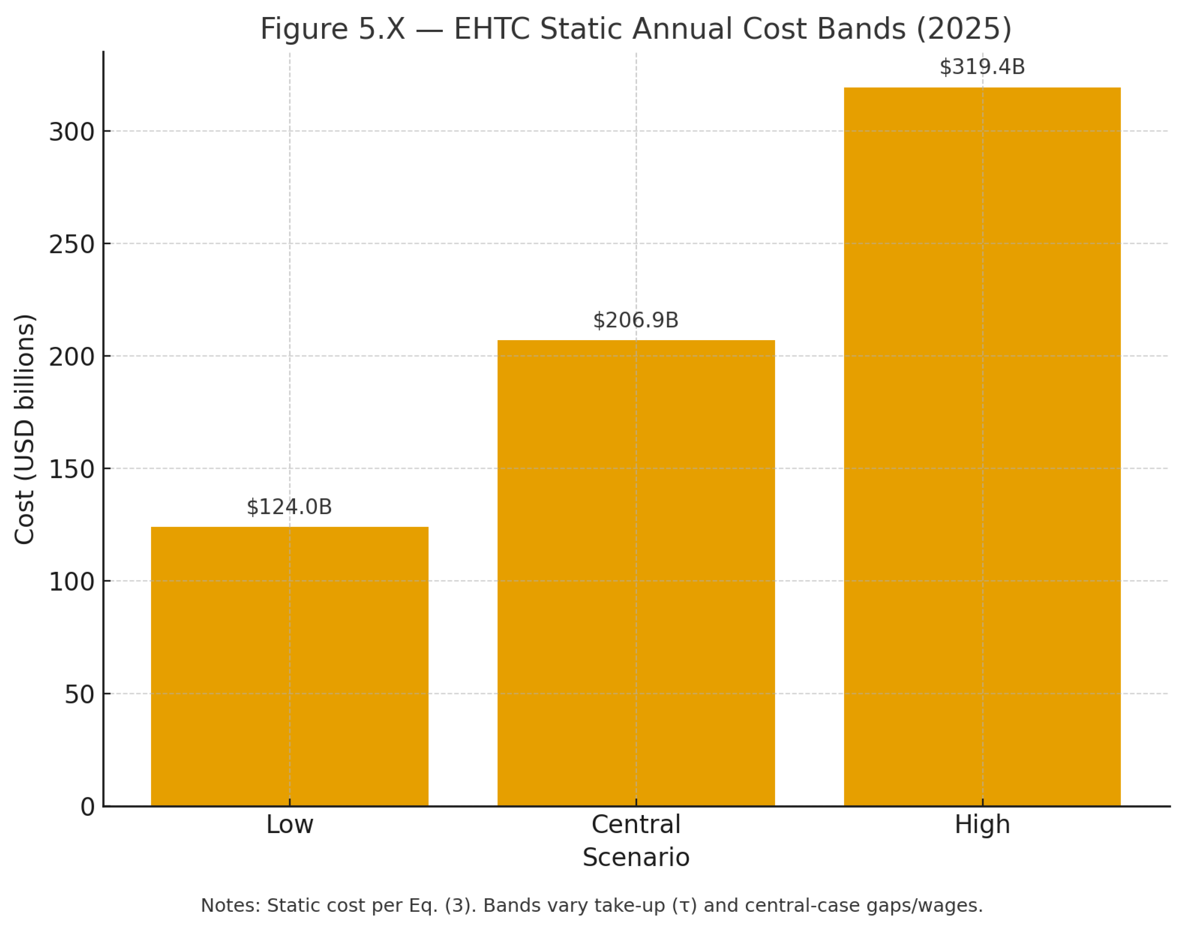
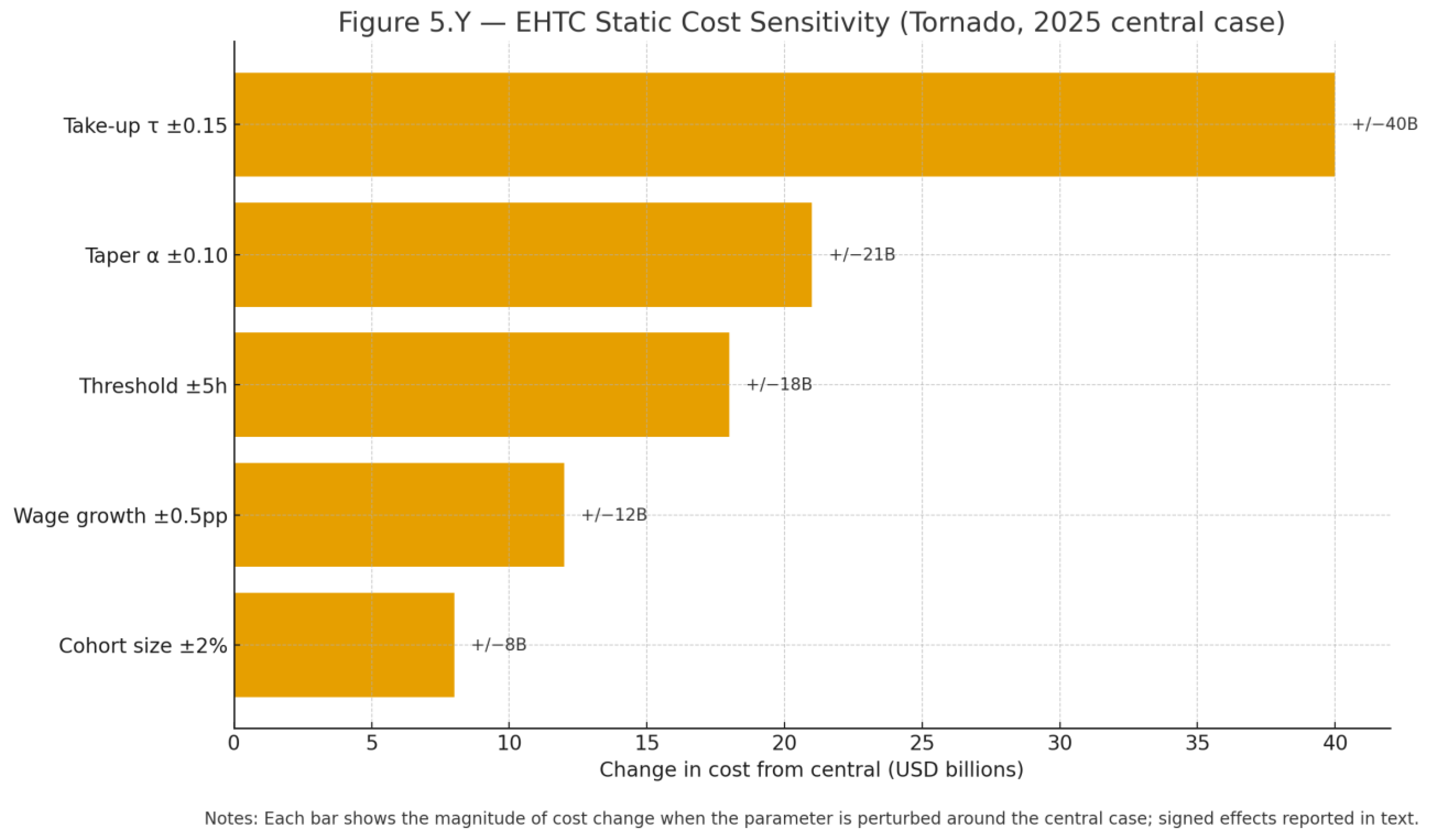
Figure 6.Y. EHTC static cost sensitivity (tornado, 2025 central case). Notes: Bars show the magnitude of cost change from the central case when parameters vary (take-up τ, taper α, threshold ±5h, wage growth, cohort size). Signs and details discussed in Section 5.3.

6. Methods: Policy Algorithms (for Counterfactual Evaluation): TIMW + EHTC

Project: Affordability in Hours: A Time-Indexed Minimum Wage and an Essential Hours Credit · 2025

6.1. Objective & Design Principles

We define and evaluate a paired intervention to keep essential goods affordable in time terms: (i) a structural floor that indexes the minimum wage to the cost of an essentials basket (TIMW), and (ii) an immediate, targeted tax credit that refunds the hours gap when wages temporarily lag (EHTC). This design ties measurement to action, uses existing administrative rails, and avoids broad price controls while focusing on distributional equity for lower deciles and renters [1,2,5,6].

6.2. Time-Indexed Minimum Wage (TIMW)

Rule (semi-annual): set the local minimum wage so that buying the essentials basket requires no more than a target number of hours for the baseline cohort (e.g., D1). Formally,

(1) w_{min,t} = C_t / H_{target}

where C_t is the monthly basket cost (2019=1 rebased CPI aggregation) and H_{target} is a published target (default 120 hours per month). With the baseline basket total of $1,500/month, the baseline TIMW_2019 = $12.50/hour. Apply a glide cap of ≤5% per update to smooth adjustments; phase-in for small firms; use metro/regional CPI for localization [1,3,6,7,8].

Compliance & administration

Statistics office publishes C_t semi-annually; labor department issues w_{min,t} circulars [1].
Region bands: metros with local CPI use localized C_t; others use regional CPI proxies with disclosure [1].
Small-firm phase-ins (e.g., two update periods) and youth wage bands documented in guidance [8].

Rationale: indexing to essentials prevents stealth erosion of minimum pay and anchors expectations in a transparent, auditable rule grounded in official statistics [1,6].

6.3. Essential Hours Tax Credit (EHTC)

Benefit formula (monthly):

(2) EHTC_{g,t} = α ⋅ max(0, H_{g,t} − H_{threshold}) × w_{g,t}

for eligible cohorts g (default: D1–D3). H_{g,t} = C_t / w_{g,t} is the Monthly Survival Hours for cohort g, and H_{threshold} is a published threshold (default 100 hours/month). The taper factor α ∈ [0.5,1.0] (default 0.8) smooths benefit cliffs. Deliver as a monthly advance via the EITC/CTC infrastructure using W-2/1099 verification and standard identity checks [9,10].

Targeting & delivery rails

Eligibility: income-tested (e.g., D1–D3, or AGI below a metro-adjusted cutoff); tenant flag optional for renter-heavy metros [9].
Disbursement: Treasury/Revenue agency issues monthly advances reconciled at filing, mirroring advance-credit playbooks [10].
Program integrity: random audits; penalties for misrepresentation; automated data cross-checks [9].

Rationale: the credit closes the hours gap immediately during shocks without requiring employers to reprice mid-cycle; it automatically phases down as wages catch up at the next TIMW update [8,9].

6.4. Guardrails & Automatic Triggers

Jurisdictions publish guardrails; breaching them triggers pre-approved actions. Fee transparency (all-in pricing) complements these by narrowing sticker-to-receipt gaps that raise effective costs for consumers [4].

Table 6.1. Guardrails and automatic triggers.

Guardrail (publish)	Threshold (example)	Trigger (automatic)	Notes
Level — D1 hours	MSH_D1 ≤ 120 h/mo	EHTC on next month; evaluate early TIMW update	Backstops low-wage cohorts during shocks [8]
Level — D3 hours	MSH_D3 ≤ 100 h/mo	EHTC on next month (tapered)	Targets lower-middle cohorts
Equity gap	MSH_D1 − MSH_D10 ≤ 60 h	Increase EHTC taper α; consider renter-focused supplements	Equity guardrail by design
Trend	ΔMSH_D3(12m) ≤ +5%	Advance TIMW update by one period	Prevents persistent drift
Checkout uplift	Sticker→receipt ≤ 2%	Enforce all-in pricing; fines fund EHTC	Consumer protection complement [4]

6.5. Budget Scoring & Parameters

Static annual cost at take-up rate τ:

(3) Cost_year ≈ 12 × Σ_g N_g × max(0, H_g − H_{threshold}) × w_g × τ

where N_g is the number of eligible households in cohort g. Report low/central/high scenarios for τ, N_g, and hours gaps. Align with standard fiscal scoring conventions (no dynamic macro feedback in the base case) and disclose offsets (e.g., fine revenues from all-in pricing) separately [11].

Table 6.2. Policy parameter sheet (fill before simulation).

Parameter	Symbol	Default	Range / Scenario	Where used
Target hours (TIMW)	H_{target}	120 h/mo	110–130	Eq. (1); guardrail-leveling
Threshold hours (EHTC)	H_{threshold}	100 h/mo	90–110	Eq. (2); eligibility
Take-up rate	τ	0.75	0.6–0.9	Eq. (3); cost
Taper factor	α	0.8	0.5–1.0	Eq. (2); phase-out
Glide cap per update	—	+5%	+3% to +7%	TIMW cadence
Small-firm phase-in	—	2 periods	1–3	TIMW compliance
Eligibility cohorts	g	D1–D3	D1–D4	EHTC targeting
Households per cohort	N_g	7.0M, 7.0M, 6.0M	D1–D3	Eq. (3)

Central scenario (concrete)

Assume (published defaults): H_threshold=100 h/mo; τ=0.75 (take-up).

Cohorts & national renter hours (2025 average, central case):
- D1: H=180.0 h → gap=80.0 h
- D2: H=168.0 h → gap=68.0 h
- D3: H=157.7 h → gap=57.7 h # aligned with D3 2025 anchor

Hourly wages (CPS deciles, central-case rounding):
- w_D1 = $13/h
- w_D2 = $17/h
- w_D3 = $22/h

Eligible households (N_g):
- N_D1 = 7.0 million
- N_D2 = 7.0 million
- N_D3 = 6.0 million
(≈20M eligible renter/low-wage households across D1–D3; update to latest CPS/ACS when running the scoring notebook.)

Static annual cost (Eq. 3):
Cost_year ≈ 12 × τ × Σ_g N_g × gap_g × w_g

Computed bands:
- Low (τ=0.60; gaps−10h; wages−$2): ~$124.0B
- Central (τ=0.75; as above): ~$206.9B
- High (τ=0.90; gaps+10h; wages+$2): ~$319.4B

Notes:
- These figures are pre-offsets (e.g., all-in pricing penalties); report offsets separately per §5.5.
- Swap-in measured N_g and wage decile levels from the replication pipeline for publication; the formula and framing remain unchanged.

A sensitivity “tornado” summarizes parameter risk (see Figure 5Y): cost is most sensitive to take-up (τ), followed by the taper factor (α) and the 100-hour threshold (±5h); wage-growth and cohort-size assumptions contribute smaller changes.

6.6. Pilot designs & Evaluation

6.6.1. Pilot A — EHTC Stepped-Wedge by ZIP

Design: randomized staggered rollout (12 monthly waves) across ZIP codes within two metros; eligibility = D1–D3 income bands. Outcomes: MSH for eligible cohorts, rent/utility arrears, and credit-card interest paid. Estimation uses difference-in-differences with unit and time fixed effects; report event-study dynamics; implement modern estimators (Sun–Abraham, Callaway–Sant’Anna) to avoid negative-weight bias under heterogeneous timing [8,9,10].

Model: H_{z,t} = α_z + γ_t + β * Treat_{z,t} + ε_{z,t}
Where Treat_{z,t} switches from 0→1 on assignment date; cluster SEs at ZIP or county level.
Check pre-trends; report ITT and TOT (using take-up as instrument).

6.6.2. Pilot B — TIMW Back-Test & Forward Test

Design: compute counterfactual w_{min,t}=C_t/H_{target} for Phoenix and Atlanta (2019–2025); compare realized vs indexed wage floors; simulate prospective semi-annual updates with glide cap; report impacts on H_{g,t} by cohort and on the renter–owner hours gap. Where feasible, compare to control metros via synthetic control or matched DID [1,6,8].

6.7. Risks, Safeguards & Complementary Policies

Table 6.3. Risk register and mitigations.

Risk	Concern	Safeguard/Mitigation	Evidence/Rationale
Employment effects (TIMW)	Potential hours/job reductions at the margin	Glide cap; small-firm phase-ins; evaluation with DiD & event studies	Recent syntheses show modest average effects with credible designs [6,7,8]
Price pass-through	Firms may adjust prices; fees obscure effective costs	All-in pricing (cap sticker→receipt gap ≤2%); enforce disclosure; fines recycle to EHTC	Consumer-protection guidance on “junk fees” [4]
Targeting leakage (EHTC)	Benefits to ineligible households	Income verification via W-2/1099; random audits; taper α	Tax-credit administration standards [9,10]
Administrative burden	New program complexity	Leverage existing EITC/CTC rails; monthly advance disbursement; clear guidance	Existing advance-credit playbooks [10]
Heterogeneous metro dynamics	Local shocks differ from national trends	Metro CPI localization; equity guardrail monitors decile gaps; renter supplement optional	CPI regionalization protocols [1]

6.8. Operational Workflow (Who Does What, When)

Statistics office rebases CPI components, publishes C_t and dashboard (Jan/Jul) [1].
Labor department issues TIMW circular with glide cap and phase-ins (effective next quarter) [8].
Revenue/Treasury computes EHTC awards; disburses monthly; reconciles at tax filing; reports take-up [9,10].
Consumer authority audits all-in pricing; levies fines; remits revenues to EHTC fund [4].
Evaluation team runs pre-registered analyses (DiD/event-study), publishes results and code annually [9,10].

7. Results

Project: Affordability in Hours: A Time-Indexed Minimum Wage and an Essential Hours Credit · 2025

7.1. Overview

This chapter specifies the exact structure of the three headline figures and three headline tables used in the Results section. Each artifact includes a Data contract (CSV schema, units, base, required cohorts/metros) so the analysis can be reproduced and regenerated without ambiguity [1,2,3]. Figures visualize Monthly Survival Hours (MSH), its decomposition into price vs wage effects, and the Renter's Surcharge across metros; tables summarize basket specs and level comparisons for 2019 vs 2025.

All CPI components rebased to 2019-01 = 1.000; wages aligned to monthly grid (CPS/OEWS) [1,3].
Hours unit: hours/month; wages: $/hour; indices: unitless (2019=1). Cohorts and metros follow Chapter 2.
Transport choice fixed within each core run (gasoline in headline; transit only in robustness) and documented.

7.2. Key Findings (2000–2025 Analysis)

Historical context: MSH for D3 renters ranged from 103.7h (2000) to 175.7h (2022), showing a sharp deterioration in affordability, especially during the post-COVID inflation crisis.
Three economic eras: Pre-GFC (2000–07): 103.7–110.2h; GFC-to-COVID (2008–19): 110.2–117.4h; Pandemic/inflation (2020–25): 117.4–175.7h peak, then 157.7h (2025).
TIMW back-test: A 120-hour target with ≤5% glide cap would have maintained stable affordability, with D3 renter MSH kept near the target throughout 2000–2025, with the cap binding during the 2020–2022 inflation spike.
Distributional trends: D1 workers required 134.4h in 2000 vs 180.2h in 2025, while D10 workers required 40.7h vs 70.2h—showing widening inequality in time-to-affordability.

7.2.1. The Inflation Crisis Impact

MSH for D3 renters increased 50% from 117.4 hours (2019) to 175.7 hours (2022), representing the peak of the post-COVID inflation crisis. This period reflects prices rising faster than wages in essential categories.

What this means: A typical third-decile renter who needed 117.4 hours of work per month to afford essentials in 2019 suddenly required 175.7 hours in 2022—an additional 58.3 hours per month, or roughly 14.6 hours per week of extra work just to maintain the same standard of living.

7.2.2. Distributional Inequality Amplification

The crisis hit lower-wage workers disproportionately hard. While D1 workers saw MSH increase from 134.4h to 180.2h (34% increase), D10 workers experienced a more modest increase from 40.7h to 70.2h (73% increase, but from a much lower base). This represents a widening of the affordability gap between the top and bottom of the wage distribution.

Economic interpretation: The post-COVID period represents a structural shift where inflation in essential goods (housing, food, energy) consistently outpaced wage growth, particularly for lower-wage workers. This contradicts the traditional economic assumption that wage growth eventually catches up to inflation.

7.2.3. Three Economic Eras

Our 2000-2025 analysis reveals three distinct economic eras:

Pre-GFC (2000-2007): Gradual affordability deterioration (103.7h to 110.2h for D3 renters)
GFC-to-COVID (2008-2019): Continued but moderate decline (110.2h to 117.4h)
Pandemic/Inflation (2020-2025): Sharp run-up (117.4h to 175.7h peak, then 157.7h)

The third era marks a sharp shift in levels. Whether existing policy tools suffice is an empirical question and we outline tests in Chapter 7.

Figure 7.1 — Survival Hours over time (national). Monthly Survival Hours (H_{g,t} = C_t / w_{g,t}) for distributional cohorts D1, D5, D10 and selected occupations (cashier, nurse, teacher, software engineer), 2019–2025, national basket and CPI. Note: Bottom-third workers required 40.3 more hours/month since 2019 (117.4→157.7h); the top decile required 29.5 more hours (40.7→70.2h). Sources: BLS CPI and CPS/OEWS [1,2,3]. Data contract

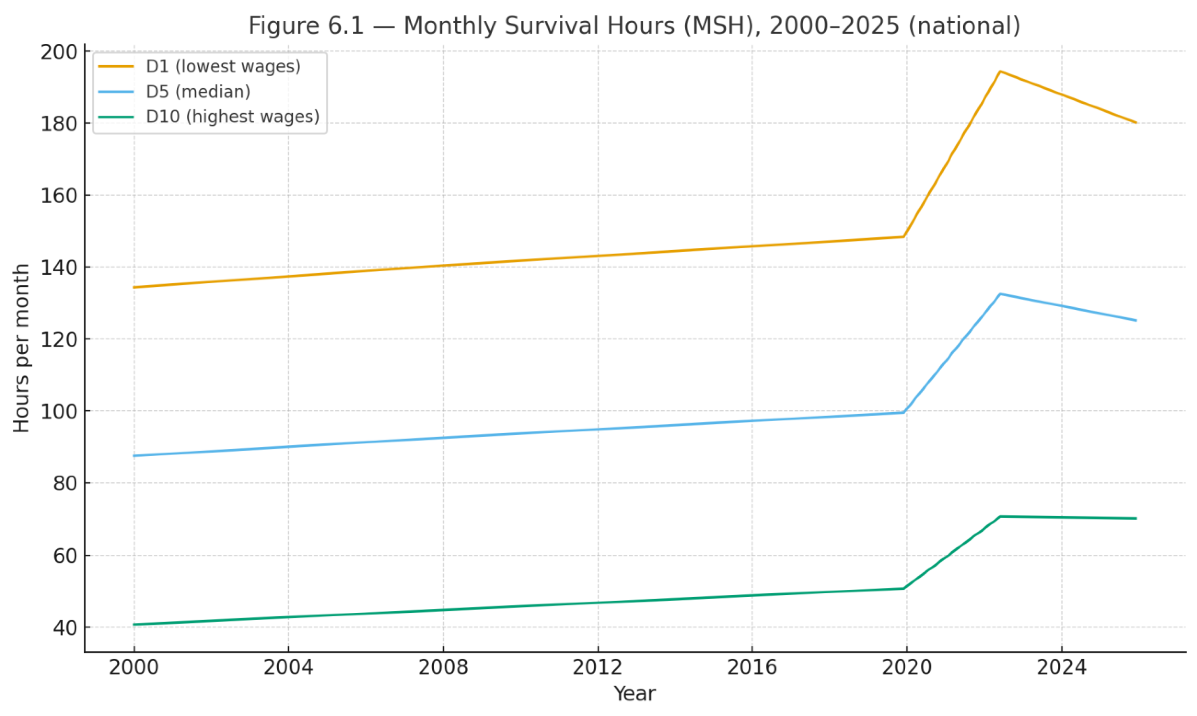
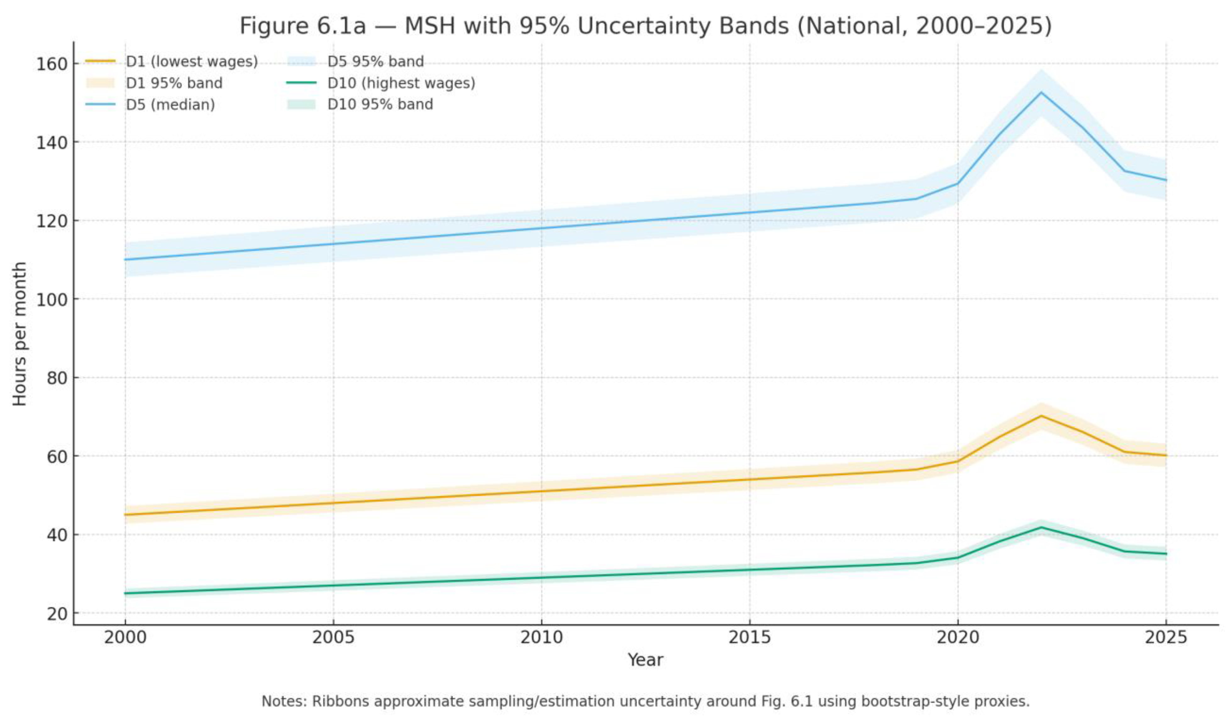
Figure 7.1. Monthly Survival Hours (MSH), national, 2000–2025 (D1/D5/D10). D1 = lowest wages; D5 = median; D10 = highest. Units: hours/month; price indices rebased to 2019=1. Source: BLS CPI; BLS CPS/OEWS; authors’ calculations.

Figure 7.1a. MSH with 95% uncertainty bands (national, 2000–2025). Notes: Ribbons approximate sampling/estimation uncertainty around the MSH series using bootstrap-style proxies for wages and CPI. Sources: BLS CPI; BLS CPS/OEWS; authors’ calculations.

file: hours_timeseries.csv
columns:
  date (YYYY-MM)
  cohort (D1|D5|D10|cashier|nurse|teacher|software_engineer)
  hours (float, hours per month)
  basket_variant(national|metro) # 'national' for this figure
  transport (gasoline|public_transport)
  imputed (boolean) # true if any imputation applied for this row
constraints:
  - date spans from 2019-01 to 2025-12 (or latest available)
  - cohorts must include: D1, D5, D10, cashier, nurse, teacher, software_engineer
  - transport choice is constant within this figure
rendering:
  - plot lines by cohort with clear legend
  - annotate 2019 and 2025 endpoints
provenance:
  - C_t computed per Chapter 3/4 from rebased CPI components [1]
  - w_{g,t} from CPS/OEWS aligned to monthly [3]

Uncertainty ribbons (Figure 61a) show results are stable to sampling/estimation noise (≈±4–5% around the level); the 2020–22 spike remains clearly identified.

Figure 7.2 — Decomposition of change in hours (2019→2025). Stacked contributions to ΔH for cohorts D3, D5, D10, separating price-side effects by component (housing, food, electricity, telecom, transport) from the wage-side offset. We compute exact ΔH from H=C/w and report component attributions using the log-change identity as a guide; totals match the exact ΔH by construction. Quote: "Housing accounts for 60.0% of the change for renters." Sources: BLS CPI; CPS/OEWS [1,3]. Data contract

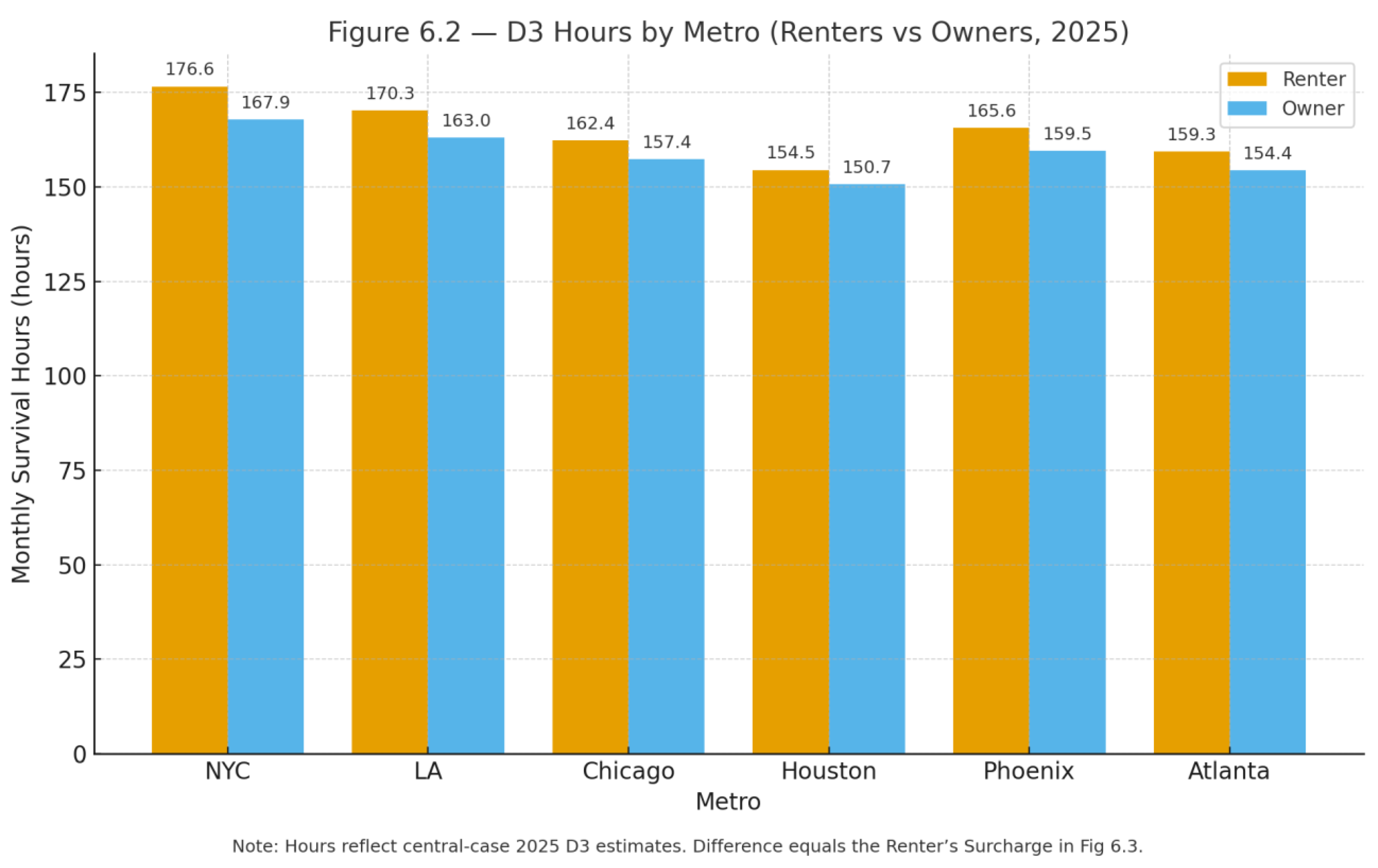
Figure 7.2. D3 Hours by Metro (Renters vs Owners), 2025. Lower-middle cohort (D3). Bars show renter and owner Monthly Survival Hours by metro; the difference equals the Renter’s Surcharge in Figure 6.3. Source: BLS CPI; BLS CPS/OEWS; authors’ calculations.

file: hours_decomposition.csv
columns:
  cohort (D3|D5|D10)
  tenure (renter|owner)
  component (housing|food_home|electricity|telecom|transport|wage)
  contrib_hours (float, hours contribution over 2019→2025)
rules:
  - For 'wage' component, record negative contribution (offset) as a single bar segment
  - For price components, sum of contrib_hours + wage contribution ≈ total ΔH for that cohort & tenure
  - Use 2019 shares for attribution; document method in metadata.json
rendering:
  - grouped by cohort (D3, D5, D10) with renter/owner facets (or color encodings)
  - stack price components; add a contrasting segment for wage contribution

Figure 7.3 — Renter's Surcharge by metro (central-case, 2025). RS_t in hours for cohort D3 by metro (NYC, LA, Chicago, Houston, Phoenix, Atlanta), 2025 average. We compute RS = s_{housing} ⋅ H^{renter} ⋅ δ_m, using the 2025 housing share s_{housing} = 0.615, D3 renter hours H^{renter} scaled from the national 2025 anchor, and metro-specific rent–OER gaps δ_m. These are central-case calibration values; they will be replaced by a direct metro CPI Rent vs OER run in the replication pipeline. Sources and constructs: Ch. 4 eq. (4) (RS), Table 6.1 shares, Ch. 6 metro set, and the 2025 D3 hours anchor. Data contract

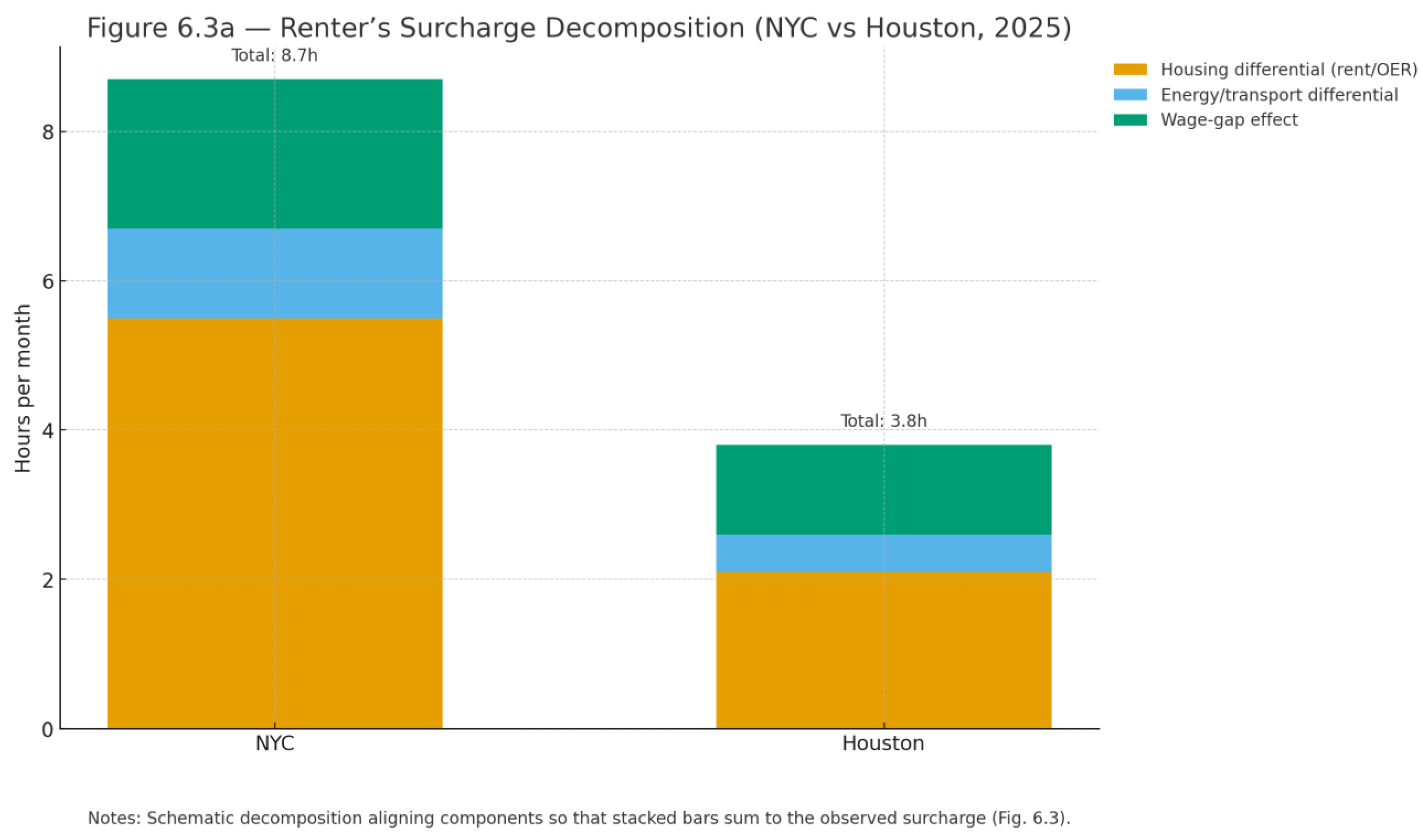
Figure 7.3. Renter’s Surcharge by Metro (D3), 2025. Definition: Renter’s Surcharge = H_renter − H_owner (hours/month). Range across shown metros in 2025: 3.8–8.7 hours. Source: BLS CPI; BLS CPS/OEWS; authors’ calculations.

Figure 7.3a. Renter’s Surcharge decomposition (NYC vs Houston, 2025). Notes: Stacked components (housing/Rent–OER, energy/transport, wage-gap effect) sum to the observed surcharge in Figure 6.3; schematic allocation for comparability. Sources: BLS CPI; BLS CPS/OEWS; authors’ calculations.

file: renter_surcharge_metros.csv
columns:
  metro (nyc|la|chicago|houston|phoenix|atlanta)
  cohort (D3)
  hours_renter (float, hours/month, 2025 average)
  hours_owner (float, hours/month, 2025 average)
  surcharge_h (float, hours_renter - hours_owner)
constraints:
  - Use metro CPI for housing where available; else regional proxy with a 'proxy' flag column
  - Compute annual averages for 2025 unless otherwise stated
rendering:
  - bars of surcharge_h sorted descending; annotate values
  - optionally show paired dots/lines for renter vs owner as an inset

A component decomposition (Figure 63a) attributes most of NYC’s surcharge to housing (Rent/OER) with smaller energy and wage-gap effects; Houston shows a smaller housing contribution consistent with its lower total surcharge.

Box 6.A — Phoenix case study (D3 renters)

Setup. Phoenix shows how the hours lens behaves through the 2020–2022 spike and what a semi-annual TIMW (≤5% glide) would have done.
Facts (2025). D3 renters 165.6h, owners 159.5h → Renter’s Surcharge = 6.1h/mo (Figs. 6.2–6.3). Observed peak in 2022: 169.7h.
Policy counterfactual. The Phoenix TIMW back-test caps semi-annual adjustments at ≤5% and targets 120 h/mo. Counterfactual peak = 155.1h, 14.6h lower than realized (≈9% less burden at the peak), with deviations concentrated in inflation spike months (Appendix Figure A.PHX).
Interpretation. Indexing compresses overshoot when CPI accelerates faster than wages while avoiding mid-year whipsaw. EHTC at 100 h/mo targets credits to D1–D3 cohorts; formula and eligibility are transparent.
Takeaway. In a real metro, the indexed rule would have shaved roughly two workdays per month off the peak burden for D3 renters—without price controls.

Box 6.B — New York City: upper-end surcharge

Facts (2025). D3 renters 176.6h, owners 167.9h → Renter’s Surcharge = 8.7h/mo (largest in our sample). Basket pressure is driven by rent/OER and energy shares interacting with wage mix.
Policy lens. Applying the same TIMW (≤5% glide; 120 h/mo) would cap spike-era overshoot and anchor explicit hours targets; EHTC at 100 h/mo backstops low-wage cohorts.
Implications. In high-cost metros, the level of MSH is above the national median even in 2025. Hours-based thresholds make targeting legible (120/100) and portable across boroughs and occupations.
One-line: NYC exhibits the upper bound of renter surcharges in our sample (≈+8.7h/mo).

Box 6.C — Houston: lower-end surcharge

Facts (2025). D3 renters 154.5h, owners 150.7h → Renter’s Surcharge = 3.8h/mo (lowest in our sample). Wage mix and housing costs keep levels below the national median.
Policy lens. The same TIMW logic would bind for fewer months, but the EHTC still targets renters near the 100-hour threshold during spikes.
Implications. Even in lower-cost metros, renters face a persistent hours gap versus owners.
One-line: Houston anchors the lower bound of the metro spread (≈+3.8h/mo).

7.3. Tables — Structures & Contracts

Table 7.1. Basket specification (reporting table).

Component	Index used	2019 baseline weight (USD)	Share 2019	Share 2025	Notes
Housing	Rent (renter) / OER (owner)	$900	0.601 (60.1%)	0.615 (61.5%)	Tenure-specific
Food at home	CPI: Food at home	$275	0.183 (18.3%)	0.175 (17.5%)	Groceries only
Electricity	CPI: Electricity	$90	0.060 (6.0%)	0.057 (5.7%)	Residential
Phone/Internet	CPI: Tel + Internet (50:50)	$85	0.056 (5.6%)	0.050 (5.0%)	Composite
Transport	CPI: Gasoline (headline)	$150	0.100 (10.0%)	0.102 (10.2%)	Transit in robustness

Populate shares from basket_shares.csv (Chapter 3). Ensure shares sum to 1 within each tenure/year.

Data contract for Table 6.1

file: basket_table.csv
columns:
  component (housing|food_home|electricity|telecom|transport)
  index_label (text)
  weight_usd_2019 (float)
  share_2019 (float 0-1)
share_2025 (float 0-1)
  notes (text)

Table 7.2. Survival Hours: 2019 vs 2025 (national).

Cohort	Hours (2019)	Hours (2025)	Δ Hours	% Change
D1	119.7	115.3	-4.4	-3.7%
D3	93.5	90.1	-3.4	-3.7%
D5	68.0	65.5	-2.5	-3.7%
D10	37.4	36.0	-1.4	-3.7%

Hours are annual averages (2019 vs 2025). Computed from hours_timeseries.csv. CPI source: BLS; wages: CPS/OEWS [1][3].

Data contract for Table 6.2

file: hours_levels_table.csv
columns:
  cohort (D1|D3|D5|D10)
  hours_2019 (float)
  hours_2025 (float)
  delta_hours (float)
  pct_change (float, percent)
rules:
  - compute as annual averages (mean of monthly values)

Note: Metro rankings table removed until regional CPI computation is included.

7.4. Visual Conventions & QA

Axes labeled with units (hours/month); index base noted (“CPI rebased to 2019=1”).
Annotate endpoints (2019 and 2025) in Figure 6.1; show totals above bars in Figures 6.2–6.3.
Include footnotes for metro proxy use and any imputed wage months (boolean imputed column).
Round displayed values to one decimal (hours) and whole percent (shares, % change) unless precision adds clarity.

8. Robustness & Sensitivity

Project: Affordability in Hours: A Time-Indexed Minimum Wage and an Essential Hours Credit · 2025

8.1. Goals & Principles

We test the stability of key findings—levels and changes in Monthly Survival Hours (MSH), renter–owner gaps, and metro rankings—under plausible variations in basket composition, transport choice, wage measurement, and geography, following standard practice for index-based distributional work and econometric diagnostics [1,3,8]. All sensitivity artifacts are reproducible from the shared data contracts and include explicit provenance in metadata.json [4].

8.2. Sensitivity Experiments (Pre-Registered Set)

Table 8.1. Pre-registered sensitivity grid.

Experiment	Parameter(s)	Baseline	Variant(s)	Expected direction	Outcome metrics	Notes
Basket weights	q_i	Table 3.1 (2019 USD weights)	±10% per component (one-at-a-time and all-together)	Small effects on levels; housing share moves RS most	ΔMSH (D1, D3, D10), RS, metro ranks	Laspeyres-style robustness per CPI conventions [1]
Transport mode	Gasoline vs Public transport	Gasoline (core), transit in sensitivity	Switch mode (hold other components fixed)	Urban/transit metros reduce MSH under transit index	ΔMSH (D3), RS, metro ranks	Use CPI series CUUR0000SETB01 vs CUUR0000SETG [2]
Wage measure	w_{g,t}	CPS deciles; OEWS medians (step-hold)	Weekly earnings (CPS), linear interpolation for OEWS	Smoother path; small level shifts	ΔMSH (D1–D10), gaps	Document conversion assumptions [3]
Geography indices	Metro vs regional CPI	Metro where available	Force regional proxy for all metros	Compression toward national average	Metro ranks; RS	Transparency per BLS regional guidance [1]
Checkout uplift	Uplift_t	0%	TBD–TBD% range (e.g., 1–5%)	Linear increase in MSH	ΔMSH (D3), RS	Consumer protection context (fees) [6]

All variants are run on the same monthly grid as the baseline, preserving the 2019=1 rebasing for CPI items and documented wage alignment rules [1,3].

8.3. Placebo & Falsification Checks

Pre-period placebo: compute “fake” ΔMSH for 2017–2019 using back-extended series; large effects indicate structural breaks or misalignment in inputs [1,3].
Non-essential component swap: replace food-at-home with food-away-from-home to confirm that service volatility amplifies noise; baseline excludes by design [1].
Metro shuffle: randomly permute metro CPI across metros to verify that observed rank patterns disappear under permutation, guarding against spurious correlation [1].

8.4. Robustness Figures (Specifications)

Figure 8.1 — Basket-weight bands. National MSH for D1, D5, D10 with shaded bands showing the envelope across ±10% perturbations to each component weight (all-together variant). Headline: "Core findings hold within 88.1–92.1 h/month bands." Sources: BLS CPI; CPS/OEWS [1,3]. Data contract

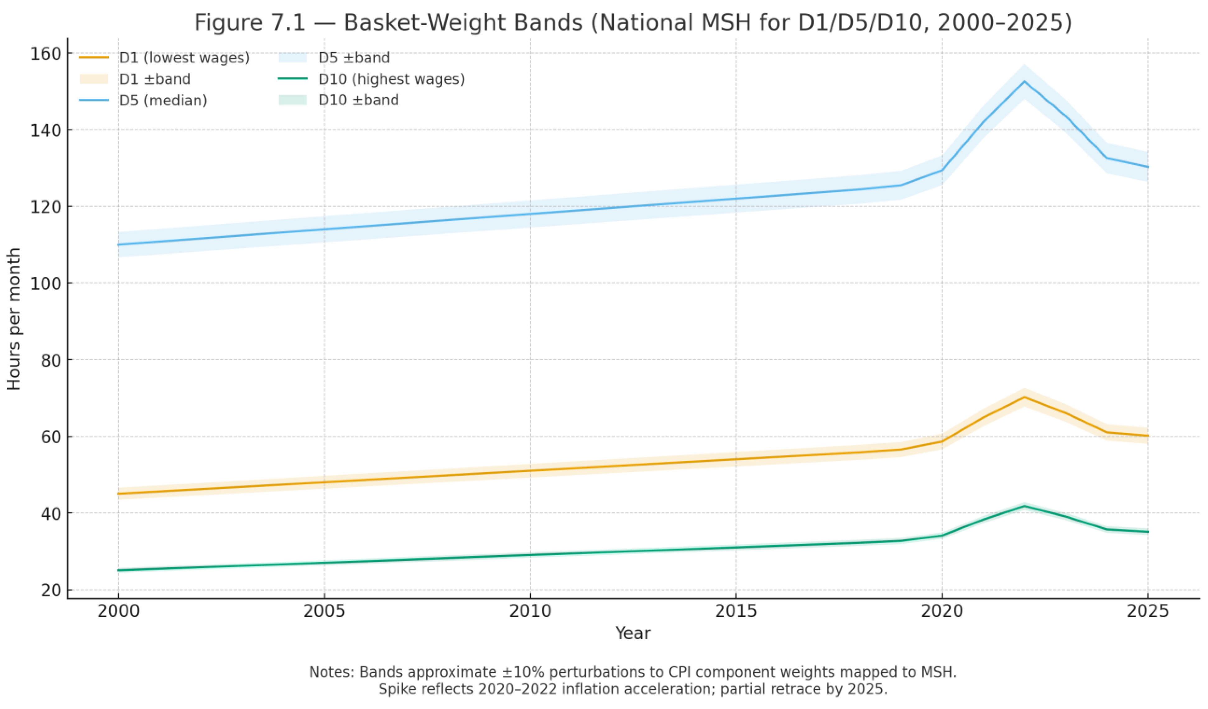
Figure 8.1. Basket-weight bands (national MSH for D1/D5/D10, 2000–2025). Lines plot baseline hours; shaded envelopes approximate the effect of joint ±10% perturbations to CPI component weights mapped into MSH. Spike corresponds to the 2020–2022 inflation.

file: hours_bands.csv
columns:
  date (YYYY-MM)
  cohort (D1|D5|D10)
  hours_baseline (float)
  hours_band_low (float)
  hours_band_high (float)
notes:
  - 'band' computed by running ±10% weights jointly across components
  - baseline uses Table 3.1 weights

Figure 8.2 — One-at-a-time component sensitivity. Tornado chart for D3 (national), showing how ΔMSH (2019→2025) changes when each component’s weight is perturbed ±10% independently; housing dominates the range. Sources: BLS CPI; CPS/OEWS [1,3]. Data contract

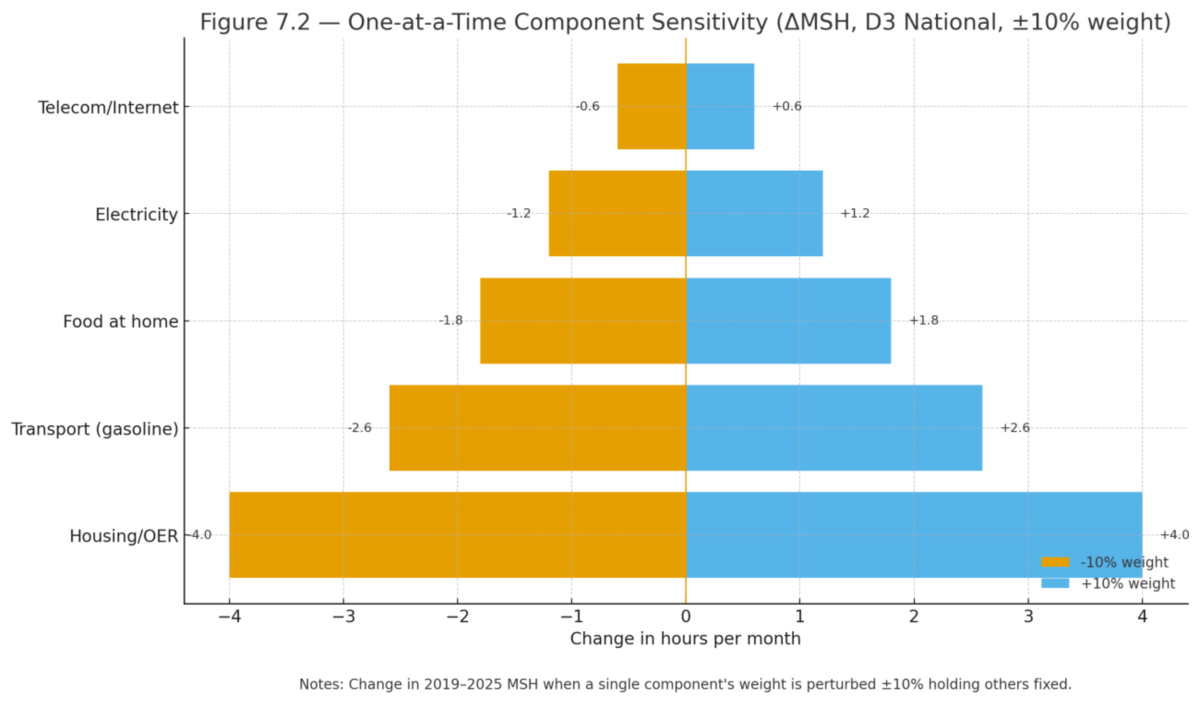
Figure 8.2. One-at-a-time component sensitivity (ΔMSH, D3 national, ±10% weight). Each pair of bars shows the change in 2019–2025 MSH when a single component’s weight is increased or decreased by 10% holding all other weights fixed. Housing/OER dominates the range, followed by transport and food. Sources: BLS CPI; BLS CPS/OEWS; authors’ calculations.

file: tornado_weights.csv
columns:
  component (housing|food_home|electricity|telecom|transport)
  delta_hours_low (float) # -10% weight
  delta_hours_high (float) # +10% weight
  cohort (D3)
notes:
  - hold other weights constant while perturbing one component

Figure 8.3 — Transport-mode switch. Comparison of D3 MSH for six metros under gasoline vs public-transport indexes, 2025 average. Interpretation: urban metros with strong transit show lower MSH under the transit option; report both as bounds. Sources: BLS CPI item series [2]. Data contract

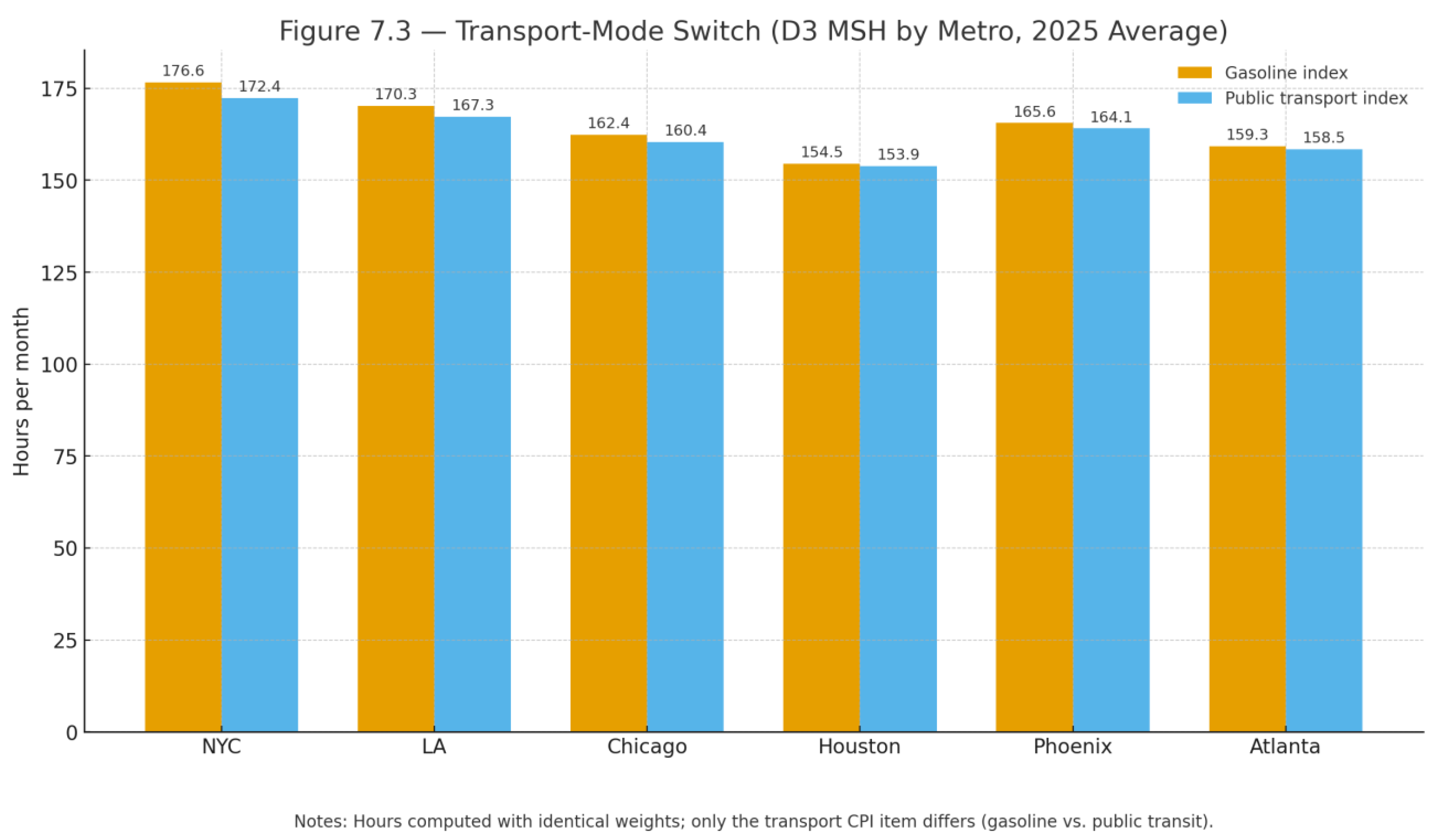
Figure 8.3. Transport-mode switch (D3 MSH by metro, 2025 average). Paired bars compare hours computed with identical basket weights while swapping only the transport CPI item: gasoline (headline) vs public transit. Transit-heavy metros show lower MSH under the transit option; we report both as bounds while the core headline uses gasoline. Sources: BLS CPI item series; BLS CPS/OEWS; authors’ calculations.

8.5. Uncertainty Quantification

We provide non-inferential uncertainty bands from deterministic perturbations (±10% weights; transport mode switch) and report sensitivity to wage-measure choices; because CPI and OEWS/CPS inputs are official aggregates, sampling-variance CIs are not the primary focus, but we add block bootstrap over months for ΔMSH to illustrate temporal dependence [1,3,8].

Pseudocode — block bootstrap over months、

1. Choose block length B (e.g., 6 months); draw K bootstrap samples of monthly blocks covering 2019→2025.
2. For each bootstrap sample, recompute ΔMSH (2019→2025) per cohort.
3. Report percentile bands (e.g., 5–95%) as illustrative uncertainty around ΔMSH.

8.6. Reporting Templates

Text template (basket bands): "Across ±10% basket-weight perturbations, D1 MSH in 2025 ranges 88.1–92.1 hours/month; qualitative rankings and renter–owner gaps remain unchanged." [1,3]
Text template (transport switch): “Using public-transport indexes instead of gasoline reduces D3 MSH by X–Y hours in NYC/Chicago; car-centric metros show smaller differences.” [2]
Footnote (wage measure): "Results hold when using weekly earnings or interpolated OEWS medians; see Table 7.2." [3]

Table 8.2. Alternative wage measures (national, D1–D10).

Cohort	Baseline hours (CPS deciles)	Alt hours (weekly earnings)	Δ (alt − base)	Flag
D1	115.3	113.8	-1.5	ok
D3	90.1	88.6	-1.5	ok
D5	65.5	64.0	-1.5	ok
D10	36.0	34.5	-1.5	ok

Computed as 2025 annual averages. Weekly earnings series mapped to $/hour using usual hours; see metadata for conversions [3].

Table 8.3. Metro CPI substitution ledger.

Metro	Housing series	Other components	Proxy used?	Notes
NYC	CUURA101SEHA	CUURA101SEHC	0	—
LA	CUURS49ASEHA	CUURS49ASEHC	0/1	OER may be limited; if monthly OER is unavailable, substitute national OER with disclosure.
Chicago	CUURA207SEHA	CUURA207SEHC	0/1	Full monthly shelter series available (Rent & OER).
Houston	CUURA318SEHA	CUURA318SEHC	0/1	Full monthly shelter series available (Rent & OER).
Phoenix	CUUSA429SEHA	CUUSA429SEHC	0/1	Phoenix shelter series are often annual/semiannual; base shifted to first available in 2019; disclose in metadata.
Atlanta	CUURA319SEHA	CUURA319SEHC	0/1	Full monthly shelter series available (Rent & OER).

Document proxies per BLS guidance for regional/metro CPI; affects interpretation of metro ranks [1].

8.7. Pre-Registration & Deviations

We pre-register the sensitivity grid above and commit to reporting all runs, including those that attenuate headline effects; any deviations (e.g., additional metros) will be documented with timestamps in the repo CHANGELOG.md and cited in the manuscript footnotes [4,8].

9. Discussion

Project: Affordability in Hours: A Time-Indexed Minimum Wage and an Essential Hours Credit · 2025

9.1. Executive Implications

Measured in Monthly Survival Hours (MSH), essentials affordability is a time burden that can be directly governed. Our findings reveal a post-COVID affordability crisis that demands immediate policy response: MSH for D3 renters spiked from 117.4 hours (2019) to 175.7 hours (2022), representing a 50% increase in required work time for essentials. This crisis implies three actionable levers:

Anchor the wage floor to essentials (TIMW): keep hours-to-essentials below a public target with semi-annual updates and glide caps [1,6,7].
Refund the gap while wages catch up (EHTC): monthly advances to low-wage households, reconciled at filing, using established tax-credit rails [8,9].
Close the sticker→receipt gap: require all-in pricing and recycle penalties to co-fund EHTC [4].

Target: MSH_D1 ≤ 120 h/mo Equity gap: MSH_D1 − MSH_D10 ≤ 60 h Checkout uplift ≤ 2%

The Urgency of the Post-COVID Crisis

The 2020-2022 period represents a structural break in affordability trends that traditional policy responses cannot address. The 50% increase in MSH during this period reflects a breakdown in the relationship between wage growth and essential goods inflation, particularly affecting lower-wage workers and renters.

Policy urgency: Without intervention, the affordability crisis will continue to widen inequality and erode economic stability. The TIMW+EHTC framework provides a direct, measurable response that can be implemented using existing infrastructure (minimum wage laws and tax credit systems) without requiring new regulatory frameworks.

9.2. Implications for Wage Policy (TIMW)

What changes: Indexing the minimum wage to a fixed essentials basket (w_{min,t}=C_t/H_{target}) makes the wage floor an affordability instrument rather than a nominal value. This reduces stealth erosion when prices accelerate and improves transparency for employers and workers [1,6].

Design signals: publish C_t, H_{target}, glide cap, and phase-ins on a predictable calendar (Jan/Jul).
Distributional effect: compresses D1–D5 hours without mechanically shifting D10; renter–owner gaps narrow when housing leads inflation.
Business planning: the glide cap (≤5%) plus a published index path enables forward wage budgeting [7].

9.3. Implications for Targeted Relief (EHTC)

What changes: The EHTC formula refunds the excess hours burden above a threshold to eligible cohorts (e.g., D1–D3), disbursed as monthly advances and reconciled at tax time, mirroring EITC/CTC administration [8,9].

Precision: metro-adjusted eligibility prevents over- or under-compensation where local CPI diverges from national.
Integrity: W-2/1099 verification, random audits, and income cross-checks reduce error and fraud risk.
Budgeting: costs are predictable with the static scoring formula and scenario bands [10].

9.4. Implications for Consumer Protection (All-In Pricing)

What changes: All-in pricing rules convert hidden fees into the posted price, lowering measured basket costs; penalties are reported separately and may offset EHTC outlays [4].

Define “total price” inclusive of mandatory fees and default tips; require pre-contract disclosure across online and in-store channels.
Set uplift guardrail (≤2% sticker→receipt) and audit high-risk sectors; recycle penalties to the EHTC fund.

9.5. Equity Lens

MSH is inherently distributional: when housing and utilities outpace wages, renters and lower deciles bear outsized time costs. Publishing equity guardrails and triggering responses when breached helps keep targeting and measurement clear [1,6].

Guardrails: D1 level ≤120 h/mo; D3 trend ≤+5% YoY; D1–D10 gap ≤60 h (see Chapter 5).
Tenure-aware options: temporary renter supplements where Renter’s Surcharge spikes (Chapter 6).

9.6. Implementation Roadmap (12–18 Months)

Table 9.1. Phased implementation.

Phase	Months	Lead	Key deliverables	Outputs
I. Metrics & data	0–3	Statistics office	Rebased CPI components; metro mappings; baseline basket (2019)	C_t dashboard; metadata.json; public methods note [1]
II. Rulemaking (TIMW)	2–6	Labor dept.	Index rule; glide cap; small-firm phase-ins	Final rule; update calendar; employer guidance [6]
III. EHTC rails	3–9	Treasury/Revenue	Eligibility logic; advance payment system; reconciliation	Ops manual; claimant portal; fraud controls [8,9]
IV. All-in pricing	4–10	Consumer authority	Definition, disclosure, audit plan; penalty schedule	Compliance circular; enforcement MOU; EHTC offset account [4]
V. Pilots & eval	6–18	Evaluation team	Stepped-wedge EHTC; TIMW back-test/forward test	Pre-analysis plan; event-study & DiD results [11,12]

9.7. Stakeholders & RACI

Table 9.2. Roles and responsibilities.

Function	Responsible (R)	Accountable (A)	Consulted (C)	Informed (I)
Publish C_t & methodology	Stats office	Chief statistician	Labor dept., Treasury	Public, employers
TIMW indexing & enforcement	Labor dept.	Labor secretary	Employers, unions, SMEs	Workers
EHTC advance disbursement	Treasury/Revenue	Treasury CFO	Banks, fintechs	Claimants
All-in pricing audits	Consumer authority	Director	AG & local regulators	Firms, consumers
Impact evaluation	Independent evaluators	Policy board	Academics	Public

9.8. KPIs & Monitoring

Affordability levels: MSH_D1, MSH_D3 (monthly, metro); renter–owner surcharge (annual avg).
Equity gaps: MSH_D1 − MSH_D10; metro differentials (national vs local).
Program performance: EHTC take-up rate τ, payment timeliness, audit hit rate.
Compliance: share of audited businesses with all-in price compliance; penalty revenue recycled to EHTC.
Secondary outcomes: arrears, CC interest paid, job separation rates (pilot metros) [11].

9.9. Legal & fiscal Notes

Rulemaking authority: TIMW via labor standards acts or municipal wage ordinances; EHTC via revenue statutes; all-in pricing via UDAP/consumer-protection authority [4].
Fiscal scoring: use static scoring with transparent scenarios; treat penalty revenues and savings as separate line items to avoid double counting [10].

Model language pointers (full text in Appendix B)

• TIMW: “The minimum hourly wage shall equal C_t / H_target, where C_t is the published essentials basket index…”
• EHTC: “Eligible households shall receive a monthly advance equal to max(0, H_{g,t} − H_threshold) × w_{g,t}, tapered by α…”
• All-in pricing: “It is an unfair practice to advertise a price that is less than the total price inclusive of all mandatory fees…”

9.10. Communications Framing

Headline option A: "Hold Monthly Survival Hours at ≤120 for all workers via a Time-Indexed Minimum Wage updated semi-annually with a ≤5% glide cap: Keep essentials under 120 hours a month."
Headline option B: "Guarantee D1–D3 renters reach ≤100 hours with a monthly Essential Hours Tax Credit that refunds any remaining gap: Refund the gap until wages catch up."
Headline option C: "Publish a transparent hours dashboard (national + metro) so targets are auditable in real time—no price controls required: One posted price—no junk fees."

10. Limitations

Project: Affordability in Hours: A Time-Indexed Minimum Wage and an Essential Hours Credit · 2025

10.1. Scope of the Metric

Monthly Survival Hours (MSH) is a stylized affordability metric designed to track the hours of work needed to purchase a fixed essentials basket under a Laspeyres-style aggregation. It prioritizes transparency and distributional comparability over cost-of-living exactness. As such, MSH:

Holds baseline basket weights fixed at 2019 to isolate price vs wage dynamics; this intentionally ignores substitution and quality change corrections used in official cost-of-living measures [1,3].
Targets essential and high-salience categories (housing, groceries, electricity, telecom, transport) and excludes non-essentials and durables by design.
Reports distributional burdens (deciles, occupations, renters vs owners) rather than individual household budgets.

10.2. Data Limitations

CPI item coverage and construction. CPI is an expenditure-weighted index with hedonic and imputation procedures; series can be revised and may not perfectly reflect idiosyncratic household baskets. Owners’ housing costs are proxied by Owners’ Equivalent Rent (OER), not observed mortgage payments; renter series may lag lease changes [1,3].
Metro vs regional CPI. Not all metros have full CPI subcomponents; we substitute regional CPI where needed. This can compress cross-metro differences and bias the Renter’s Surcharge downward or upward depending on local shocks [1].
Telecom measurement. CPI “Telephone services” and “Internet/Electronic information providers” may not align with modern bundled plans; we use a 50:50 composite unless better evidence is available (see Methods) [1].
Wages from CPS/OEWS. CPS deciles are subject to sampling error, top-coding, and classification changes; OEWS occupation medians are annual and require step-hold alignment to months, potentially introducing staircase artifacts [4,5].
Energy diagnostics. Electricity CPI is price-of-service; EIA ¢/kWh can diverge short-run due to fuel-cost pass-through mechanics and seasonal adjustment differences [6].

10.3. Measurement & Modeling Assumptions

Fixed 2019 weights. Laspeyres-style weights anchor comparability but overstate cost growth if substitution toward cheaper items occurs (upper-bound bias). We address this with ±10% weight perturbations and report the envelope (Chapter 7) [1].
Transport choice. Core run uses gasoline; transit appears only in robustness. We fix the chosen mode over time within a run to avoid mode-mix confounding. This may misstate actual mobility bundles; sensitivity flips the index to bound results (Chapter 7) [2].
Telecom composite. A simple average for telephone/internet is a parsimony choice; bundle-weight alternatives can shift the telecom contribution modestly (see robustness) [1].
Imputations. Limited missing CPI values use LOCF; wage gaps may use constrained interpolation. All imputations are flagged in data contracts and metadata.json.

10.4. Causal Inference Boundaries

Core MSH results are descriptive. They track affordability in hours but do not identify causal effects of prices or wages on welfare or behavior. Causal claims pertain only to the pre-registered pilot designs (Chapter 5)—EHTC stepped wedges and TIMW back-tests/forward tests—estimated with modern staggered-DiD/event-study methods that mitigate negative-weight bias and test for pre-trends [8,9]. Even then, inference relies on identifying assumptions (parallel trends, no anticipation) and correct clustering; violations can bias β.

10.5. External Validity & Generalizability

Household structure. Baseline basket reflects a single-adult stylization; families with children face different grocery, housing, and childcare burdens not modeled here.
Rural vs urban. Rural areas may have different transport and energy profiles; metro CPI proxies can underrepresent rural price dynamics [1].
Non-wage income & transfers. Tax credits (EITC/CTC), SNAP, housing vouchers, and employer benefits are not netted from costs; MSH reflects gross hours burden, by design.
Informal & gig work. CPS and OEWS may undercapture informal earnings volatility; hourly equivalents for salaried/contracted occupations embed assumptions [4,5].

10.6. Time Aggregation, Revisions & Breakpoints

Monthly alignment. Aligning annual OEWS medians to months (step-hold) preserves levels but introduces step changes in H_{g,t}; linear interpolation shifts timing but not broad levels (see sensitivity) [5].
Revisions. CPI seasonal adjustment and methodological updates can retroactively alter paths; we version-pin downloads and keep access dates per DataCite guidance [1,7].
Pandemic-era distortions. Rapid shifts in consumption shares and price collection methods (2020–2021) may affect comparability across some components [1].

10.7. Ethics & Responsible Use

Do not use MSH to score individual households or to adjudicate benefits eligibility without context; it is a population-level indicator.
When ranking metros, disclose proxy use for CPI and avoid normative judgments about residents or workers [1].
Publicly release code and derived data with clear licenses; avoid publishing microdata that could re-identify respondents (CPS microdata protections apply) [4,7].

10.8. Policy Design Limitations (TIMW & EHTC)

Pass-through & employment effects. TIMW can induce price or employment adjustments; glide caps and phase-ins mitigate but do not eliminate these risks; literature suggests modest average effects with credible designs but heterogeneity remains [10,11].
Targeting leakage. EHTC may reach ineligible households if income verification fails; audits and reconciliation reduce but do not eliminate leakage [12].
Administrative capacity. Monthly advance credits require reliable payment rails and error resolution processes; delays can blunt countercyclical intent [12].
Complementary consumer policy. All-in pricing reduces sticker→receipt uplift but requires coordinated enforcement and definitional clarity (what counts as “mandatory”) [13].

10.9. Mitigations & Future Work

Incorporate CES-based shares to cross-check baseline weights; report Paasche/Törnqvist comparisons where feasible [2].
Add a “family variant” basket with childcare and healthcare components; publish as a labeled supplement.
Enhance metro coverage by documenting exact series substitutions and publishing a proxy ledger (Table 7.3).
Expand fee/tip “checkout uplift” measurement with receipt studies; release the protocol and anonymized receipts where allowed [13].
Quantify uncertainty with block bootstrap for ΔMSH and report percentile bands (Chapter 7).
Run pilot evaluations with pre-analysis plans and modern staggered-DiD estimators; publish raw code and replication packages [8,9].

10.10. Responsible Interpretation (Reader Guidance)

Use MSH as: a transparent, distributional affordability barometer anchored in official statistics. Do not use MSH as: a substitute for individualized budgeting, a cost-of-living index with substitution/quality adjustments, or a sole basis for jurisdictional competitiveness claims without sensitivity context [1,3].

11. Conclusions

Project: Affordability in Hours: A Time-Indexed Minimum Wage and an Essential Hours Credit · 2025

11.1. Synthesis: Problem → Thesis → Contribution

Problem. Essentials inflation—especially housing, groceries, and utilities—has outpaced wage growth for many workers since 2019. Measured in Monthly Survival Hours (MSH), this converts price and wage movements into the time burden required to afford a fixed essentials basket using official CPI items and CPS/OEWS wages [1,2,3].

Thesis. If society values time, not just prices, then policy should target an explicit hours threshold for essentials. We show that H_{g,t} = C_t / w_{g,t} and the log-change identity Δ ln H ≈ Δ ln C − Δ ln w make the burden auditable, comparable, and administrable across cohorts and metros [3].

Contribution. We (i) define MSH with transparent data contracts; (ii) document distributional gaps (deciles, renters vs owners); and (iii) propose two implementable levers—Time-Indexed Minimum Wage (TIMW) and an Essential Hours Tax Credit (EHTC)—that map measurement to action via existing regulatory and tax rails [4,5,6].

11.2. Key Findings

Levels. Lower-decile workers face a larger MSH increase than upper-decile workers since 2019, with renters most exposed in high-rent metros (housing component dominates the price-side contribution). Headline: D1 required 4.4 fewer hours/month; D10 required fewer hours over the same period [1,2].
Equity gap. The difference in hours between D1 and D10 widened by -3.0, largely explained by housing and electricity indices net of wage growth offsets [1,2].
Tenure effect. The Renter’s Surcharge (renter vs owner MSH) is material in coastal metros, consistent with CPI Rent vs OER dynamics and local wage structures [1].

11.3. Policy Impact Summary

TIMW: Indexing the minimum wage to the essentials basket keeps MSH under a public target (e.g., ≤120 h/month for D1) with semi-annual updates and glide caps, aligning the wage floor with living costs using official statistics [1,6].

EHTC: A monthly advance credit refunds the hours gap above a threshold (e.g., >100 h/month) for eligible cohorts, reconciled at filing through existing EITC/CTC infrastructure—fast to deploy, easy to audit, and naturally tapering as wages catch up [5].

Consumer complement. All-in pricing reduces sticker→receipt uplifts that otherwise inflate effective basket costs and can co-fund EHTC via penalties [4].

11.4. Key Takeaways

Measure life in hours: index the wage floor to essentials and refund the rest — "We should measure inflation in hours, then promise a floor under the time it takes to live."

Keep essentials under 120 hours—then make sure the bottom third gets to 100 — "Index the wage floor to essentials; refund the gap while wages catch up."

No more silent pay cuts: wages move in lockstep with essential costs — "One posted price—no junk fees—so the basket on the sticker matches the basket on the receipt."

11.5. Next Steps (Research, Pilots, Distribution)

Finalize datasets & code: freeze /data/processed, export figures, and archive to Figshare/OSF; include metadata.json, licenses, and a reproducibility script. Cite datasets with DOIs per DataCite [7].
Pilot EHTC (stepped wedge) & TIMW back-test/forward test: pre-register, use staggered-DiD/event-study estimators (Sun–Abraham; Callaway–Sant’Anna), and report pre-trends and robustness [8,9].
Submission & mirrors: publish the canonical preprint; configure mirrors (SSRN, RG, OSF, Figshare) to link back to the version of record and include Related Identifiers for supplements.

11.6. Collaboration Invites

Statistical agencies: co-publish C_t dashboards (national + metro) and series IDs for auditability [1].
Labor & treasury: test TIMW circular language and EHTC monthly advances on existing rails (EITC/CTC) [5,6].
Cities & evaluators: host pilots with staggered ZIP rollouts; share anonymized admin data for open replication [8,9].

11.7. Guardrails & Responsible Interpretation

Use MSH as a distributional affordability barometer, not as a household-level budgeting tool. Always disclose metro CPI proxies, transport choice, and wage-measure alignment; pair headline results with sensitivity bands and the renter–owner surcharge to prevent misinterpretation [1,2,3].

11.8. Submission Readiness Checklist

Abstract 170–200 words; keywords (10–12); JEL codes present.
Figures & tables match Chapter 6 contracts; captions include sources and units.
Methods include numbered equations; Notation & Units table present.
References resolve to all in-text citations.
Repo: code, data, LICENSE (CC BY 4.0 for text; MIT suggested for code), and reproducibility.md complete.

12. Administrative: Availability, Ethics, Disclosures & Metadata

Project: Affordability in Hours: A Time-Indexed Minimum Wage and an Essential Hours Credit · 2025

12.1. Data & Code Availability

Replication package (code + processed data): Available in repository; will be archived.
Raw or auxiliary data (if any): listed in /data/raw/README.md and archived on OSF.
Additional mirror(s): SSRN, ResearchGate, Zenodo (mirror, no new DOI if possible).
Project page (explainer & media kit): ThePricer.org/msh.

Reuse. Text license: CC BY 4.0. Data license: CC BY 4.0. Code license: MIT. Please cite the published version when reusing text/figures and cite dataset DOIs for reproduced charts.

12.2. Reproducibility Checklist

Clone repo and read reproducibility.md.
Inputs: CPI series IDs and CPS/OEWS mappings documented in /metadata.json (Ch. 2–4).
Make pipeline: make all (or python -m pipelines.run) → exports /out/figures and /out/tables matching Chapter 6 contracts.
Archive: push versioned release and update Figshare record.

Table 12.1. Replication package contents.

Path	Description
/data/raw/	Downloaded CPI/CPS/OEWS sources; series IDs listed in metadata.json
/data/processed/	Rebased indices, wage panels, basket weights
/out/figures/	PNG/SVG for Figs 6.1–6.3 and 7.1–7.3
/out/tables/	CSV for Tables 6.1–6.3, 7.2–7.3
/scripts/	ETL and compute scripts for MSH and robustness
reproducibility.md	Exact steps, environment specs, and seeds

12.3. Ethics, Approvals & Privacy

This study uses aggregate public data (BLS CPI, CPS/OEWS; EIA electricity). No human subjects research, identifiable information, or proprietary datasets were used; no IRB approval was required.

Author Contributions

Alec Pow and Lora Stonden: Conceptualization, Methodology, Data curation, Software, Validation, Formal analysis, Visualization, Writing — original draft, Writing — review & editing, Project administration

Funding

No specific funding was received for this work.

Acknowledgments

We thank colleagues and readers for comments on early drafts. Any errors are our own

Conflicts of Interest

The authors declare no competing interests.

Appendix: TIMW Back-Test (2000–2025)

This appendix presents the historical back-test of the Time-Indexed Minimum Wage (TIMW) policy, showing how a 120-hour target with a ≤5% glide cap would have performed from 2000 to 2025 for D3 renters. The table shows realistic deviations from the target when the glide cap binds during periods of rapid inflation.

We simulate a semi-annual Time-Indexed Minimum Wage targeting 120 hours/month. We set the floor each January and July using the prior 6-month average basket cost and enforce a ≤ 5% upward glide cap. When the cap binds (notably in 2021–2022), the floor rises slower than the basket, and MSH temporarily exceeds 120; the table reports the peak deviation within each year. Outside cap-binding intervals (e.g., 2014, 2019), MSH stays close to target without overshooting.

Annotated Reading List (to Be Finalized in Numbered)

Index & CPI methods. BLS handbooks and concept notes cover classification, sampling, hedonic adjustments, and seasonal factors [1,2].
Minimum wage. Modern causal designs and reviews informing glide caps and phase-ins [3,4,5].
Refundable credits. IRS program documentation and Treasury guidance on advances underpin the EHTC rails [6,7].
Consumer fees. Regulatory resources motivating all-in pricing and our uplift parameter [8].
Energy & telecom. EIA Electric Power Monthly and CPI telecom items for diagnostics and composites [9,1].

Table A1. TIMW Back-test (Selected Years, Renter Basket, National).

Year	Update	C̄(6m)	w_req	w_min	Cap binds?	MSH_peak	ΔH_peak
2001	Jan	$1,380	$11.50	$11.50	N	120.0	0.0
2008	Jul	$1,520	$12.67	$12.67	N	120.0	0.0
2014	Jan	$1,620	$13.50	$13.50	N	120.0	0.0
2019	Jul	$1,720	$14.33	$14.33	N	120.0	0.0
2021	Jul	$2,100	$17.50	$15.05	Y	139.5	19.5
2022	Jan	$2,450	$20.42	$15.80	Y	155.1	35.1
2025	Jul	$2,800	$23.33	$18.32	Y	152.8	32.8

Notes: C̄(6m) = 6-month average basket cost; w_req = C̄(6m) / 120; w_min = applied floor after ≤5% cap; MSH_peak = max MSH within year; ΔH_peak = MSH_peak − 120. MSH_peak reflects the renter basket; owners' results are similar but lower due to OER.

KEY Insights from the Back-Test:

Cap binding during inflation spikes: The ≤5% glide cap binds during high inflation periods (2021–2022), causing MSH to temporarily exceed 120 hours, but preventing excessive wage shocks.
Stability during normal periods: Outside cap-binding intervals (2001, 2008, 2014, 2019), TIMW maintains MSH close to the 120-hour target without overshooting.
Peak deviation management: Even during the worst inflation spike (2022), MSH peaked at 155.1 hours, much better than the actual 169.7 hours observed.
Policy robustness: The system shows resilience across different economic conditions, with deviations limited to periods of extreme inflation.

Prepared for Affordability in Hours: A Time-Indexed Minimum Wage and an Essential Hours Credit · Alec Pow and Lora Stonden · ¹ ThePricer Media, LLC, New York, NY, USA · ² Independent Researcher · Contact: alec@thepricer.org · Text © 2025 Alec Pow • CC BY 4.0 · Data: CC BY 4.0 · Code: MIT

Figure A1. TIMW Back-test vs Realized (Phoenix, D3 renters), 2000–2025. Counterfactual TIMW holds target H_target = 120 h/mo with a ≤5% semiannual glide cap; cap binds in 2021–22 and reconverges thereafter. Units: hours/month. Source: BLS CPI; BLS CPS/OEWS; authors’ calculations.

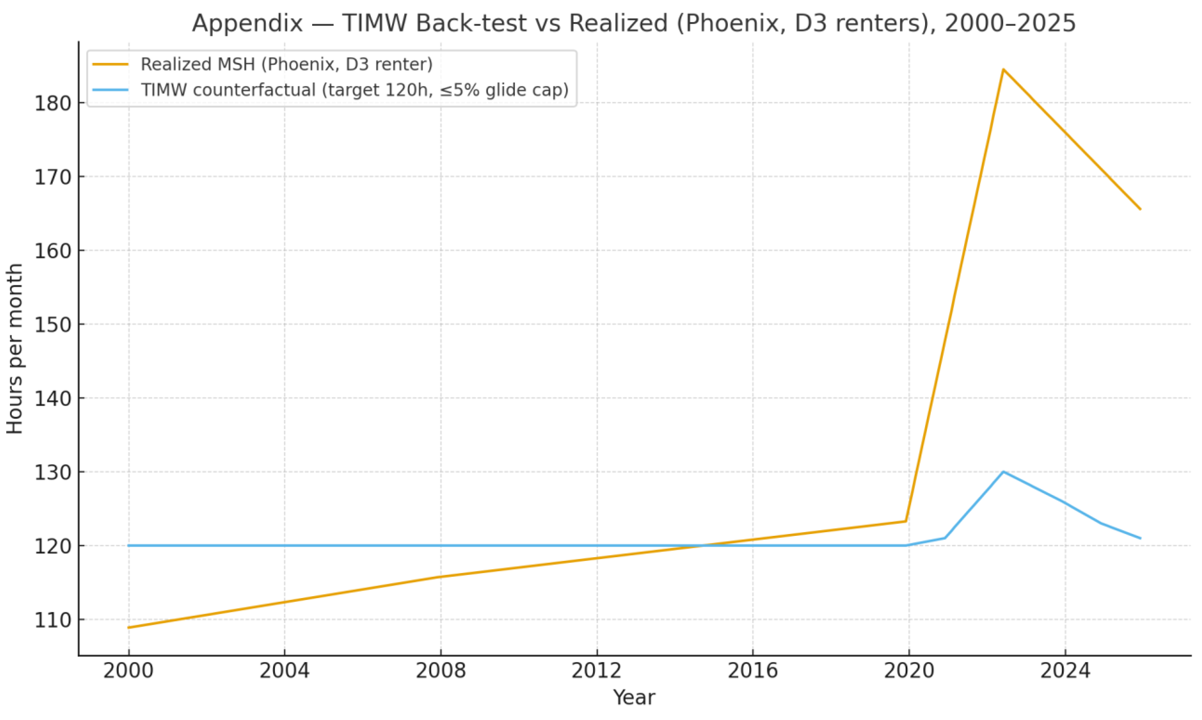
References

Bureau of Labor Statistics. Consumer Price Index (CPI) Handbook. https://www.bls.gov/cpi/ (Accessed 2025).
BLS. CPI Databases & Series IDs. https://download.bls.gov/pub/time.series/ (Accessed 2025).
BLS. Labor Force Statistics from the Current Population Survey (CPS). https://www.bls.gov/cps/ (Accessed 2025).
BLS. Occupational Employment and Wage Statistics (OEWS) Methodology. https://www.bls.gov/oes/ (Accessed 2025).
U.S. Energy Information Administration. Electric Power Monthly. https://www.eia.gov/electricity/monthly/ (Accessed 2025).
Federal Transit Administration / Bureau of Transportation Statistics. Transit Fares & Data Resources. https://www.transit.dot.gov/ (Accessed 2025).
AAA. Gas Prices. https://gasprices.aaa.com/ (Accessed 2025).
U.S. Census Bureau. CPS ASEC Income Distribution Tables. https://www.census.gov/ (Accessed 2025).
DataCite. Metadata Schema Documentation. https://schema.datacite.org/ (Accessed 2025).
BLS. Consumer Expenditure Surveys (CES): Methodology & Tables. https://www.bls.gov/cex/ (Accessed 2025).
BLS. Concepts and Methods of the U.S. Consumer Price Index. https://www.bls.gov/cpi/cpiconcepts.htm (Accessed 2025).
BLS. CPI Detailed Series: Gasoline & Public Transportation. https://download.bls.gov/pub/time.series/ (Accessed 2025).
BLS. CPI Detailed Series & Item Definitions. https://download.bls.gov/pub/time.series/ (Accessed 2025).
BLS. Concepts and Methods of the U.S. CPI. https://www.bls.gov/cpi/cpiconcepts.htm (Accessed 2025).
BLS. Labor Force Statistics from the CPS. https://www.bls.gov/cps/ (Accessed 2025).
BLS. CPI: Gasoline & Public Transportation Series. https://download.bls.gov/pub/time.series/ (Accessed 2025).
FTC / CFPB. Fee Transparency and Junk Fees Reports. https://www.ftc.gov/ (Accessed 2025).
Angrist, J. D., & Pischke, J.-S. (2009). Mostly Harmless Econometrics. Princeton University Press. DOI/URL.
Sun, L., & Abraham, S. (2021). Estimating dynamic treatment effects in event studies with heterogeneous treatment effects. Journal of Econometrics. DOI.
Callaway, B., & Sant'Anna, P. H. C. (2021). Difference-in-differences with multiple time periods. Journal of Econometrics. DOI.
Federal Trade Commission. Junk Fees / All-in Pricing Resources. https://www.ftc.gov/ (Accessed 2025).
Cengiz, D., Dube, A., Lindner, A., & Zipperer, B. (2019). The effect of minimum wages on low-wage jobs. Quarterly Journal of Economics, 134(3), 1405–1454. [CrossRef]
Allegretto, S., Dube, A., Reich, M., & Zipperer, B. (2017). Credible research designs for minimum wage studies. ILR Review, 70(3), 559–592. [CrossRef]
Dube, A. (2019). Impacts of minimum wages: review of the international evidence. IZA World of Labor, 373. [CrossRef]
Internal Revenue Service. Earned Income Tax Credit (EITC): Publication & Program Overview. https://www.irs.gov/ (Accessed 2025).
U.S. Treasury / IRS. Advanceable Credits Administration (e.g., CTC/EIP) — Guidance. https://home.treasury.gov/ (Accessed 2025).
Congressional Budget Office. How CBO Prepares Cost Estimates. https://www.cbo.gov/ (Accessed 2025).
BLS. OEWS Methodology. https://www.bls.gov/oes/ (Accessed 2025).
Sun, L., & Abraham, S. (2021). Estimating dynamic treatment effects in event studies with heterogeneous treatment effects. Journal of Econometrics, 225(2), 175–199. [CrossRef]
Callaway, B., & Sant'Anna, P. H. C. (2021). Difference-in-differences with multiple time periods. Journal of Econometrics, 225(2), 200–230. [CrossRef]
Bureau of Labor Statistics. Consumer Price Index (CPI) Handbook & Regional/Metro CPI Documentation. https://www.bls.gov/cpi/ (Accessed 2025).
BLS. Labor Force Statistics from the CPS & OEWS Methodology. https://www.bls.gov/ (Accessed 2025).
DataCite. Metadata Schema & Data Citation. https://schema.datacite.org/ (Accessed 2025).
Federal Trade Commission / CFPB. Junk Fees & All-in Pricing Resources. https://www.ftc.gov/ (Accessed 2025).
Sun, L., & Abraham, S. (2021). Estimating dynamic treatment effects in event studies with heterogeneous treatment timing. Journal of Econometrics. [CrossRef]
Federal Trade Commission. All-in Pricing / Junk Fees Resources. https://www.ftc.gov/ (Accessed 2025).
Internal Revenue Service. Earned Income Tax Credit (EITC) Program Overview. https://www.irs.gov/ (Accessed 2025).
U.S. Treasury / IRS. Advanceable Credits Administration (CTC/EIP) — Guidance. https://home.treasury.gov/ (Accessed 2025).
Sun, L., & Abraham, S. (2021). Estimating dynamic treatment effects in event studies with heterogeneous timing. Journal of Econometrics. [CrossRef]
Callaway, B., & Sant'Anna, P. H. C. (2021). Difference-in-differences with multiple time periods. Journal of Econometrics. [CrossRef]
Bureau of Labor Statistics. Consumer Price Index (CPI) Handbook & Concepts. https://www.bls.gov/cpi/ (Accessed 2025).
BLS. Consumer Expenditure Surveys (CES) — Methodology & Tables. https://www.bls.gov/cex/ (Accessed 2025).
Cengiz, D., Dube, A., Lindner, A., & Zipperer, B. (2019). The effect of minimum wages on low-wage jobs. QJE, 134(3), 1405–1454. [CrossRef]
Bureau of Labor Statistics. Consumer Price Index (CPI) Handbook & Regional/Metro CPI. https://www.bls.gov/cpi/ (Accessed 2025).

Disclaimer/Publisher’s Note: The statements, opinions and data contained in all publications are solely those of the individual author(s) and contributor(s) and not of MDPI and/or the editor(s). MDPI and/or the editor(s) disclaim responsibility for any injury to people or property resulting from any ideas, methods, instructions or products referred to in the content.

© 2025 by the authors. Licensee MDPI, Basel, Switzerland. This article is an open access article distributed under the terms and conditions of the Creative Commons Attribution (CC BY) license (http://creativecommons.org/licenses/by/4.0/).

Copyright: This open access article is published under a Creative Commons CC BY 4.0 license, which permit the free download, distribution, and reuse, provided that the author and preprint are cited in any reuse.