
Submitted:
21 October 2025
Posted:
22 October 2025
You are already at the latest version
Abstract
Baseline correction techniques are highly applicable in analytical chemistry. Consequently, there is a constant demand for universal and automated baseline correction methods. Our new procedure based on the Convolutional Autoencoder model (ConvAuto model) combined with an automated algorithm to Apply the Model (ApplyModel procedure) meets those expectations. The key advantage of this idea is its ability to handle 1D signals of various lengths and resolutions, which is a common limitation encountered for deep neural network models. The proposed procedure is fully automatic and does not require any parameter optimization. As our experiments have shown, the ApplyModel procedure can also be easily combined with other baseline correction methods that utilize deep neural networks, such as the ResUNet model, which extended it practical application too. The usability of our new approach was tested by its implementation for both simulated and experimental signals, ranging from 200 to 4000 point length. The results were compared with those provided by the ResUNet model.
Keywords:
baseline correction
; deep neural networks
; convolutional autoencoder
; voltammetry
1. Introduction
In analytical chemistry, baseline correction is a crucial step in signal processing. The baseline refers to the signal level observed when no analyte is present or when the analyte concentration is negligible. However, due to various factors, such as instrument noise, drift, or interference substances, the baseline might not be perfectly flat. The baseline correction aims to remove these fluctuations to improve the accuracy and reliability of the analysis.
The essential approach to baseline correction involves estimating a line using polynomials. This can be accomplished through polynomials of various degrees [1] or using automatic iterative methods with polynomial fitting [2,3]. Similar to polynomials are splines, with a particular focus on cubic splines [4] and cubic Hermite splines [5,6]. Among the various ideas, worth noticing is an iterative algorithm with two-stage iteratively reweighted smoothing splines with Tukey’s Bisquare weights [7], as well as a penalized spline smoothing method based on vector transformation that helps distinguish baseline regions from peaks [8]. Another procedure incorporating splines is introduced by S. He et al. [4], where a genetic algorithm was applied to select the background spectral wavenumbers and finally fit the baseline with a cubic smoothing spline. Similarly, another approach [9] involved selecting peak regions with discrete wavelet transform in combination with the spline baseline approximation in the wavelet domain. In addition to polynomials and spline techniques, other baseline correction procedures incorporating robust baseline elimination approaches with local regression [10] and community information [11], nonquadratic cost functions [12,13] or application of sparse Bayesian learning [14] have also been introduced.
One of the most important baseline correction methods are Penalized Least Squares (PLS), which based on the Wittaker Smoother introduced by Eilers [15]. These methods have a major benefit in efficiently handling missing data points in long stretches, controlled by iteratively generated weights, with shape and smoothness adjusted mainly by a single parameter. There are a few variants of PLS methods such as Asymmetric Penalized Least Squares (AsPLS) [16,17,18,19] and adaptive iteratively reweighted Penalized Least Squares (airPLS) [20,21], with the main focus on weights minimalization, enhancing baseline correction results. Particularly interesting is the asymmetrically reweighted Penalized Least Squares (arPLS) method proposed by Beak et al. [18], which incorporates a general logistic function to iteratively adjust weights to noise levels, what help to avoid assigning a noisy baseline as small peaks. Therefore, it made the arPLS method less vulnerable to noise and more effective when applied to actual signals.
Today, Deep Learning (DL) has become a method of particular interest in various fields of science and engineering, offering powerful tools for data analysis, modelling, and prediction. DL has also emerged as a transformative tool in analytical chemistry, enhancing the precision, efficiency, and scope of chemical analysis. Classification and detection is one of the analytical problems, where DL has found significant interest. There is an application of DL in the detection of blood diseases by haemoglobin concentration [22], detection of liver cancer cells [23], distinguishing of honey sessional changes [24] and the classification of iron ore [25]. Deep Neural Networks (DNNs) are also useful for the detection of patterns and biomarkers in complex metabolomic [26] and proteomic [27] analysis incorporating big data. The SR-UNet algorithm [28] is proposed in ion trap mass spectrometry for low-resolution overlapping ion-peaks spectra to improve their resolution while ensuring sufficient sensitivity and analysis speed. DL methods also improve quantitative analysis, applying the DeepSpectra model for Raman spectroscopy [29] and enhance gas sensing below LOD [30]. They are also applicable in filtering signals from noise, improving the signal-to-noise ratio in NMR spectroscopy [31] and detection of false peaks (and distortions) for LC-MS [32].
Despite the potential, there has been a limited interest in the application of DL for baseline correction compared to other signal processing methods so far. This may be due to a lack of comprehensive signal databases, which must include both signals and their true baselines, crucial for DNN model training. In one of the few solutions, Liu Y. [33] proposed application of a model incorporating adversarial nets to recognise the baseline regions in real data, called Baseline Recognition Nets (BRN). Another method introduced multiscale analysis and regression to design a CNN model of mixed encoder – decoder architecture to generate a baseline [34]. Authors of other publication [35] used cascaded deep convolutional neural networks based on ResNet and UNet architectures, capable of full access to baseline-corrected and denoised Ramman spectra. An intriguing approach for baseline correction was introduced by Chen T. et al. [36], utilizing a DL model that merges ResNet and UNet, known as the ResUNet model. The model was trained with simulated signals. Although the method was applied to Raman spectra, it has potential to be incorporated with other analytical signals.
Therefore, to address the restricted application of DNN models in baseline correction, we have developed an authorial method based on the Convolutional Autoencoder (ConvAuto) model. This approach includes an automated procedure called ApplyModel, which facilitates the baseline correction for 1D signals of various lengths and resolutions, representing a fundamental aspect of the proposed solution. As it turned out, this solution proved to be effective in baseline correction for both simulation and experimental signals.
2. Methodology
2.1. Convolutional Autoencoder Model
The autoencoder is a particular DNN structure made of two parts, encoder and decoder. The encoder extracts features of the input signal and decomposes them into small pieces of information encoded within this part of the model. On the other hand, the decoder takes those pieces of information and combined them into an output signal, corresponding to the input signal. The encoder and decoder exchange information in the narrower part of the autoencoder called the bottleneck. Such a structure makes autoencoder as a generalization model which extracts the main features of the input signals, reconstructing them only on the basis of the most important features passing through the bottleneck. Sometimes, this is used to reconstruct the input signal without interference such as noise. In our solution, we also did not expect to reconstruct the original signals, but to design an autoencoder model which, based on the input signal, generated the baseline of this signal.
Convolutional 1D layers were used as better suited to decompose and store spatial information of signals (baseline shape, peaks locations and heights, etc.). Transposed convolutional 1D layers were applied to reconstruct those signals, respectively. The schema of the proposed Convolutional Autoencoder (ConvAuto) model is presented in Figure 1. All layers had output with ReLU activation and were normalized with batch normalization. To limit overfitting, dropout (0.2) was applied, and average pooling layers were introduced to improve model generalisation. The model kernel size was not constant, but varied progressively (see Figure 1), from 15 for input (and output) layers to 3 in the bottleneck.
DNN models have to deal with the vanishing gradient problem, which occurs during the backpropagation training mechanism. It significantly reduces the gradient, which may completely disappear if the model has many hidden layers. This was also the case for the ConvAuto model, especially in the encoder part. Therefore, to improve the learning rate and reduce prediction error, skip connections were implemented in the model structure. Thay were also made of convolutional 1D (or transposed convolutional 1D) layers with kernel size 1.
2.2. Apply Model Algorithm
A significant constraint in the broad application of baseline correction DNN models is the fixed input size imposed by the model architecture and the designated training dataset. It means that only signal with specific length, the same as model input size (in ConvAuto it was 512), can be provided into such model. Theoretically, we can imagine training as many models as possible to fit each signal length, but that is not the point. Such a solution is a waste of time and resources, requiring a countless number of datasets to train those models. Therefore, a simple algorithm (called ApplyModel) was prepared, enabling the application of the ConvAuto model to a wide range of 1D signals. The schema of this procedure is presented in Figure 2.
The ApplyModel procedure was primarily based on the adjustment of signals length to the model input size, which was basically a combination of two operations: artificial increasing (or decreasing) signal resolution; extrapolation of additional points at the beginning and ending of the signal. For increasing signal resolution, the procedures calculated the mean of two adjacent points and used this value to create a new point between those two adjacent points. It was repeated throughout the signals and the resolution was doubled. Similarly, to reduce signal resolution, the procedure just discarded even points throughout the signal and received doubled reduced resolution. These actions were repeated as many times as necessary, usually 0-3 times for one signal. However, these modifications were never enough to adjust the length of the signals to the required model input size of 512. Therefore, further adjustments were made by polynomial extrapolating additional points at the beginning and end of the signals. It applied low-level polynomials (1 or 2 degree) and used selected points from signals to approximate polynomials and then extrapolated new additional points. Thus, by combination of these two simple operations, any signal length could be adjusted to model input size 512. Certainly, such modifications influenced signals greatly (destroying peak details), but they maintained the original shape, which was enough for our ConvAuto model to generate baselines. Importantly, the procedure records all operations conducted on the original signals, which have been used to reverse all length modifications in subsequent actions.
After length adjustments, the signals were normalized (the ConvAuto model required normalized signals), and the min-max values were saved for future operations (described below). Finally, such signals were applied to the ConvAuto model, and baselines were generated. From this point on, all further operations of the ApplyModel algorithm were carried out on the generated baselines, to transform them to the original signal length. Therefore, data obtained from signal normalization and length adjustment were used here for this purpose. As the model returned normalized baselines, the denormalization operation was first performed using the min-max values obtained in the signal normalisation. Then, length adjustments were made on the generated baselines to meet the original signal length. It was done using the same methods as for signal adjustment length, but here conducted in reverse order. After that operation, the baselines matched the original signal length and were ready for baseline correction.
The ApplyModel algorithm was fully automated and did not require any parameter optimization. In addition, the algorithm was such coded that other models (like ResUNet) can be easily used here in place of ConvAuto, which was shown in the Results and Discussion section.
3. Model Preparation
3.1. Generation of Simulated Signals for Model Training
The process of developing and training DNN models presents significant challenges, mostly in maintaining a balance between the accuracy of the result and generalizability of the model. A fundamental aspect of this process involves the acquisition of a comprehensive training dataset. However, gathering such dataset is time-consuming and expensive, especially if substantial quantities of experimental signals are expected. Thus, a better idea was to generate a large number of simulation signals which were then divided into a separated training, validation and test dataset. To facilitate this, an automated procedure for generating simulated signals was established, as illustrated in Figure 3. The algorithm consists of a combination of peak, baseline, and noise generators. The first generator employed the Gaussian function (1) to calculate peak-shaped signals:
where a, p, and w were the amplitude, position, and width of the peak, respectively. It generated from 1 to 4 peaks in one signal. Their position, height, and width were randomly selected within the defined range. The baseline generator used four different methods to generate random baselines, such as cubic splines, cubic smoothing splines, polynomials (2 degree) and combination of two polynomials with non-integer exponents. The selection of the method was randomised every time the generator function was called. Baseline values were limited to the specified range. Furthermore, splines-based methods used randomly located nodes (3 to 5 nodes) to shape the baselines. The noise generator returned white noise, generated with a random amplitude within the range 0.5 – 2% of the average intensity of the peaks in the signal. Ultimately, the algorithm generated pairs of simulated signals along with their corresponding baselines. This process resulted in a training set of 105k simulated signals, as well as validation and test datasets, each consisting of 22.6k simulated signals.
3.2. Model Training Details
The model was trained on Kaggle.com platform using GPU P100 accelerator, with TensorFlow python library. Application of the final model was conducted on MSI laptop with Intel i7, Geforce 3070 RTX and 16 GB of RAM. To maintain the best memory management, all datasets were loaded and saved as TensorFlow datasets tf. Before saving the tf datasets, all signals were normalized and expanded with additional dimension (to 3D tensor), required for convolutional 1D layers.
The model training procedure started with loading train, validation and test tf datasets, which were immediately pre-fetched and shuffled (except test dataset). The input size was 512 (training signal length) and the batch size was set to 100. The model was trained in 60 epochs with Adam optimizer. The Mean Absolute Error (MAE) was used as a loss function and the Root Mean Square Error (RMSE) as metrics. The initial learning rate was 10-4 and after 5 epochs decreased exponentially by the factor of -0.1 with each epoch. Changes in loss and learning rate values during the model training procedure were gathered in Figure 4.
3.3. Experimental Signals
In addition to the test dataset, the ConvAuto model was also evaluated using two separate sets of experimental voltammetric signals, each obtained from different measurements.
The first experiment concerned the determination of Pb(II) in samples with certified concentration of Pb(II) 25.0 ± 0.1 µg.l-1 (CRM SPS-SW2, National Institute of Standards and Technology, USA). Measurements were carried out with the Differential Pulse Anodic Stripping Voltammetry (DPASV) technique, using a 2-electrode system with Rapidly Renewable Silver Annular Band Electrodes (RAgABE, with area 0.06 cm2) [37] as a working electrode and Silver Quasi-Reference Electrode (AgQRE, with area 2 cm2) as a combined reference and counter electrode. The CRM was tested without any pretreatment. To 0.5 ml of CRM SPS-SW2, 1 ml of the supporting electrolyte (mixture of 0.5 ml of 0.1 M HNO3 and 0.5 ml of 0.1 M KCl) was added and filled with distilled water to the final volume of 5 ml. The measurements were performed without removal of oxygen. The DPASV measurements procedure was conducted in 3 steps: conditioning the RAgABE by applying the potentials Econd= -800 mV, tcond= 8 s; the preconcentration step by applying the potential Eacc= -700 mV for 60 s; after 5 s of a rest period and finally recording of the voltammograms. The analysis was performed using the standard addition method. The first signal was recorded for pure CRM and the subsequent with the addition of 0.75, 1.50, 2.25 and 3 µg.l-1 of Pb(II). The standard solution of 1000 mg1-1 Pb(II) (Fluka) was analytical grade. The other experimental parameters were as follows: potential step = 2 mV, pulse potential E = 30 mV, time of potential step 20 ms (10 ms waiting time and 10 ms sampling time).
The second experiment concerned registration of highly overlapping signals for the digital signal separation procedure [38]. One of such highly overlapping signals was a mixture of ferulic, syringic and vanillic acid. The voltammograms were registered with the Differential Pulse Voltammetry (DPV) technique in a classical 3-electrode system, where Boron-Doped Diamond Electrode (BDD, Windsor Scientific Ltd., φ = 3 mm) was used as a working electrode, a double junction Ag/AgCl/3M KCl (filled with 2.5 M KNO3) as a reference electrode and a platinum rod as a counter electrode. All measurements were carried out in 5 ml of 0.2M H3PO4, used as supporting electrolyte, not deaerated. All chemicals were analytical grade. The 10 mM standard stock solution of the syringic acid was prepared by dissolving solid acid (95%, Sigma Aldrich) in ethanol (96%, POCH S.A.). Standard solutions of ferulic (99% trans-ferulic, Sigma-Aldrich) and vanillic acid (97%, Sigma Aldrich) were prepared in the same manner. Before each series of measurements, the BDD electrode was activated with Eact = 1500 mV for 5 minutes, in the supporting electrolyte. After a few seconds of rest period, the DP voltammograms were registered. The other experimental parameters were as follows: potential step = 2 mV, pulse potential E = 50 mV, time of potential step 40 ms (20 ms waiting time and 20 ms sampling time). Finally, a set of overlapping voltammograms of ferulic, syringic, and vanillic acid was registered in the concentration range of 1.15 – 5.80, 0.60 – 3.00, 0.50 – 2.50 mg.l-1 respectively.
4. Results and Discussion
The ConvAuto model was trained using the parameters outlined in Section 3.2., with the final results collected in Table 1. The low loss values observed for the three datasets (particularly test loss) demonstrated that the model was trained and prepared effectively for the baseline generation task. The observed disparity between the training loss and the other losses can be attributed to the presence of dropout layers within the model, which affected the training process and led to increase in training loss values (also training metrics).
The applicability of the model was evaluated using simulated set of signals. Selected examples of its application were gathered and depicted in Figure 5. The ConvAuto model with the ApplyModel procedure proved to be applicable to generate baselines for signals with a wide range of lengths, from 200 to 4000 data points. The baselines were generated fully automatically, without changing any parameters of the ApplyModel procedure. This is the most important feature of our baseline correction solution. It was carried out in the following order. First, the signals were adjusted to the input model size (512 points). Then, they were applied to the model which generated each baseline. The baselines were then adjusted to the original signal length, and the baseline correction was performed. It took less than 10 seconds to generate several baselines, regardless of whether the signals had 200 or 4000 points.
Furthermore, we conducted a comparative analysis of the results provided by our ConvAuto model with those produced by the ResUNet model. The ResUNet model was trained according to the recommendations of the authors [36] with our simulated datasets. The ApplyModel procedure was also used here, replacing our ConvAuto model with the ResUNet model, which was not a problem. The ApplyModel procedure was designed so that the model can be easily swapped. The results of the comparison were collected in Table 2. The ResUNet model generated slightly better baselines for the first two sets of simulated signals (SimSet 1 and 2). On the other hand, the ConvAuto model provided more accurate baselines for SimSet 3 and much better for SimSet 4. Observing the results of the baseline generation, we concluded that our ConvAuto model generated much smoother baselines. The ResUNet intruded much more noise into whole baselines, especially for baseline fragments under the peaks locations (see Figure 6). In our opinion, it could be related to the dropout and pooling layers presented in our ConvAuto model, which improved the generalization of the model and the lack of such layers in ResUNet.
Subsequently, the model was deployed on experimental voltammetric signals. The first experiment was the determination of CRM 25.0 ± 0.1 µg.l-1 Pb(II) in a sample with the standard addition method (Figure 7A). After generating baselines using our ConvAuto model, the concentration of Pb(II) was calculated as 22.4 µg.l-1, what gave recovery of 89.6%. On the other hand, with the baseline generation provided by the ResUNet, Pb(II) concentration was calculated as 22.2 µg.l-1 (recovery 88.6%). This has shown a slight advantage of our model. The second experimental set of signals was a mixture of three phenolic acids (ferulic, syringic, and vanillic acid) registered as highly overlapping signals (Figure 7B). Our automated procedure successfully generated and corrected baselines and signals could have been applied for further analysis with the multivariate method or peak separation [38].
A thorough evaluation of the ConvAuto model has also revealed some flaws in the generation of baselines. Problems sometimes manifested with the generation of noisy fragments, which usually concentrated on the first and last points of the baselines (like in Figure 8A). Sometimes the model also generated a baseline with fragments that under- or overfitted the real baseline (Figure 8B). These issues could be attributed to the extensive but finite size of the training dataset, which was not sufficiently diverse to encapsulate all conceivable baseline combinations. Significant enlargement of the training dataset is expected to reduce the frequency of these errors, but this would significantly increase training costs.
5. Summary
An innovative approach for the baseline correction of 1D signals has been proposed using the Convolutional Autoencoder (ConvAuto) model integrated with the ApplyModel procedure. The ApplyModel algorithm facilitated the direct implementation of the model for the baseline correction of 1D signals of various lengths. The evaluation of the algorithm revealed its effectiveness in handling signals ranging from 200 to 4000 points. The procedure was fully automatic, eliminating any need for parameter optimization. In addition, the ApplyModel algorithm was designed to be universal, enabling its application with other baseline correction models like ResUNet.
The model was trained with datasets consisting of self-generated simulated signals. The ConvAuto model was effectively employed in the generation of baseline for both simulated and actual signals. These operations were subsequently compared to those achieved with the ResUNet model. The evaluations indicated that our model was suitable for baseline correction, delivering results comparable or superior to ResUNet. However, some limitations of the ConvAuto model were also identified and discussed.
Funding
The research project was financed by a subsidy from the Ministry of Science and Higher Education of Poland for the AGH University of Krakow (project nr 16.16.160.557).
Declaration of generative AI and AI-assisted technologies in the writing process
During the preparation of this work the authors used Writefull tool in order to improve the readability and language of the manuscript. After using this tool, the authors reviewed and edited the content as needed and takes full responsibility for the content of the published article.
Acknowledgments
The authors thank Dr. Wanda Sordoń from AGH University of Krakow for providing the voltammetric measurement results.
Conflicts of Interest
The authors declare that they have no known competing financial interests or personal relationships that could have appeared to influence the work reported in this paper.
References
- Gallo, C.; Capozzi, V.; Lasalvia, M.; Perna, G. An algorithm for estimation of background signal of Raman spectra from biological cell samples using polynomial functions of different degrees. Vib Spectrosc 2016, 83, 132–137. [Google Scholar] [CrossRef]
- Gan, F.; Ruan, G.; Mo, J. Baseline correction by improved iterative polynomial fitting with automatic threshold. Chemometrics and Intelligent Laboratory Systems 2006, 82, 59–65. [Google Scholar] [CrossRef]
- Górski, Ł.; Ciepiela, F.; Jakubowska, M. Automatic baseline correction in voltammetry. Electrochim Acta 2014, 136, 195–203. [Google Scholar] [CrossRef]
- He, S.; Fang, S.; Liu, X.; Zhang, W.; Xie, W.; Zhang, H.; Wei, D.; Fu, W.; Pei, D. Investigation of a genetic algorithm based cubic spline smoothing for baseline correction of Raman spectra. Chemometrics and Intelligent Laboratory Systems 2016, 152, 1–9. [Google Scholar] [CrossRef]
- yin Dong, Z.; hang Yu, Z. ; Baseline correction using morphological and iterative local extremum (MILE). Chemometrics and Intelligent Laboratory Systems 2023, 240, 104908. [Google Scholar] [CrossRef]
- Chen, H.; Shi, X.; He, Y.; Zhang, W. Automatic background correction method for laser-induced breakdown spectroscopy. Spectrochim Acta Part B At Spectrosc 2023, 208, 106763. [Google Scholar] [CrossRef]
- Wei, J.; Zhu, C.; Zhang, Z.M.; He, P. Two-stage iteratively reweighted smoothing splines for baseline correction. Chemometrics and Intelligent Laboratory Systems 2022, 227, 104606. [Google Scholar] [CrossRef]
- Cai, Y.; Yang, C.; Xu, D.; Gui, W. Baseline correction for Raman spectra using penalized spline smoothing based on vector transformation. Analytical Methods 2018, 10, 3525–3533. [Google Scholar] [CrossRef]
- Górski, L.; Ciepiela, F.; Jakubowska, M.; Kubiak, W.W. ; Baseline correction in standard addition voltammetry by discrete wavelet transform and splines. Electroanalysis 2011, 23, 2658–2667. [Google Scholar] [CrossRef]
- Ruckstuhl, A.F.; Jacobson, M.P.; Field, R.W.; Dodd, J.A. Baseline subtraction using robust local regression estimation. J Quant Spectrosc Radiat Transf 2001, 68, 179–193. [Google Scholar] [CrossRef]
- Wu, Y. Gao Q.; Zhang Y. A robust baseline elimination method based on community information. Digital Signal Processing: A Review Journal 2015, 40, 53–62. [Google Scholar] [CrossRef]
- Johannsen, F.; Drescher, M. Background removal from rapid-scan EPR spectra of nitroxide-based spin labels by minimizing non-quadratic cost functions. J Magn Reson Open 2023, 16–17, 100121. [Google Scholar] [CrossRef]
- Mazet, V.; Carteret, C.; Brie, D.; Idier, J. Humbert B. Background removal from spectra by designing and minimising a non-quadratic cost function. Chemometrics and Intelligent Laboratory Systems 2005, 76, 121–133. [Google Scholar] [CrossRef]
- Li, H.; Dai, J.; Pan, T.; Chang, C.; So, H.C. Sparse Bayesian learning approach for baseline correction. Chemometrics and Intelligent Laboratory Systems 2020, 204, 104088. [Google Scholar] [CrossRef]
- Eilers, P.H.C. A perfect smoother. Anal Chem 2003, 75, 3631–3636. [Google Scholar] [CrossRef]
- Eilers, P.H.C.; Boelens, H.F.M. Baseline Correction with Asymmetric Least Squares Smoothing, Leiden University Medical Centre Report 2005. Available online: http://www.science.uva.nl/~hboelens/publications/draftpub/Eilers_2005.pdf (accessed on 16 April 2025).
- Peng, J.; Peng, S.; Jiang, A.; Wei, J.; Li, C.; Tan, J. Asymmetric least squares for multiple spectra baseline correction. Anal Chim Acta 2010, 683, 63–68. [Google Scholar] [CrossRef] [PubMed]
- Baek, S.-J.; Park, A.; Ahn, Y.-J.; Choo, J. Baseline correction using asymmetrically reweighted penalized least squares smoothing. Analyst 2015, 140, 250–257. [Google Scholar] [CrossRef] [PubMed]
- Zhang, Q.; Li, H.; Xiao, H.; Zhang, J.; Li, X.; Yang, R. An improved PD-AsLS method for baseline estimation in EDXRF analysis. Analytical Methods 2021, 13, 2037–2043. [Google Scholar] [CrossRef]
- Zhang, Z.M.; Chen, S.; Liang, Y.Z. Baseline correction using adaptive iteratively reweighted penalized least squares. Analyst 2010, 135, 1138–1146. [Google Scholar] [CrossRef]
- Zhang, F.; Tang, X.; Tong, A.; Wang, B.; Wang, J.; Lv, Y.; Tang, C.; Wang, J. Baseline correction for infrared spectra using adaptive smoothness parameter penalized least squares method. Spectroscopy Letters 2020, 53, 222–233. [Google Scholar] [CrossRef]
- Fu, H.; Tian, Y.; Zha, G.; Xiao, X.; Zhu, H.; Zhang, Q.; Yu, C.; Sun, W.; Li, C.M.; Wei, L.; Chen, P.; Cao, C. Microstrip isoelectric focusing with deep learning for simultaneous screening of diabetes, anemia, and thalassemia. Anal Chim Acta 2024, 1312, 342696. [Google Scholar] [CrossRef]
- Shuyun, W.; Lin, F.; Pan, C.; Zhang, Q.; Tao, H.; Fan, M.; Xu, L.; Kong, K.V.; Chen, Y.; Lin, D.; Feng, S. Laser tweezer Raman spectroscopy combined with deep neural networks for identification of liver cancer cells. Talanta 2023, 264, 124753. [Google Scholar] [CrossRef]
- Wójcik, S.; Ciepiela, F.; Baś, B.; Jakubowska, M. Deep learning assisted distinguishing of honey seasonal changes using quadruple voltammetric electrodes. Talanta 2022, 241, 123213. [Google Scholar] [CrossRef] [PubMed]
- Zhao, W.; Li, C.; Yan, C.; Min, H.; An, Y.; Liu, S. Interpretable deep learning-assisted laser-induced breakdown spectroscopy for brand classification of iron ores. Anal Chim Acta 2021, 1166, 338574. [Google Scholar] [CrossRef] [PubMed]
- Date, Y.; Kikuchi, J. Application of a Deep Neural Network to Metabolomics Studies and Its Performance in Determining Important Variables. Anal Chem 2018, 90, 1805–1810. [Google Scholar] [CrossRef] [PubMed]
- Lin, L.; Li, C.; Zhang, T.; Xia, C.; Bai, Q.; Jin, L.; Shen, Y. An in silico scheme for optimizing the enzymatic acquisition of natural biologically active peptides based on machine learning and virtual digestion, Anal Chim Acta 2024, 1298, 342419. [CrossRef]
- Ai, J.; Zhao, W.; Yu, Q.; Qian, X.; Zhou, J.; Huo, X.; Tang, F. SR-Unet: A Super-Resolution Algorithm for Ion Trap Mass Spectrometers Based on the Deep Neural Network. Anal Chem 2023, 95, 17407–17415. [Google Scholar] [CrossRef]
- Zhang, X.; Lin, T.; Xu, J.; Luo, X.; Ying, Y. DeepSpectra: An end-to-end deep learning approach for quantitative spectral analysis. Anal Chim Acta 2019, 1058, 48–57. [Google Scholar] [CrossRef]
- Cho, S.Y.; Lee, Y.; Lee, S.; Kang, H.; Kim, J.; Choi, J.; Ryu, J.; Joo, H.; Jung, H.T.; Kim, J. Finding Hidden Signals in Chemical Sensors Using Deep Learning. Anal Chem 2020, 92, 6529–6537. [Google Scholar] [CrossRef]
- Wu, K.; Luo, J.; Zeng, Q.; Dong, X.; Chen, J.; Zhan, C.; Chen, Z.; Lin, Y. Improvement in signal-to-noise ratio of liquid-state NMR spectroscopy via a deep neural network DN-Unet. Anal Chem 2021, 93, 1377–1382. [Google Scholar] [CrossRef]
- Kantz, E.D. , Tiwari S., Watrous J.D., Cheng S., Jain M. Deep Neural Networks for Classification of LC-MS Spectral Peaks. Anal Chem 2019, 91, 12407–12413. [Google Scholar] [CrossRef]
- Liu, Y. Adversarial nets for baseline correction in spectra processing. Chemometrics and Intelligent Laboratory Systems 2021, 213, 104317. [Google Scholar] [CrossRef]
- Jiao, Q.; Guo, X.; Liu, M.; Kong, L.; Hui, M.; Dong, L.; Zhao, Y. Deep learning baseline correction method via multi-scale analysis and regression. Chemometrics and Intelligent Laboratory Systems 2023, 235, 104779. [Google Scholar] [CrossRef]
- Kazemzadeh, M.; Martinez-Calderon, M.; Xu, W.; Chamley, L.W.; Hisey, C.L.; Broderick, N.G.R. Cascaded Deep Convolutional Neural Networks as Improved Methods of Preprocessing Raman Spectroscopy Data. Anal Chem 2022, 94, 12907–12918. [Google Scholar] [CrossRef] [PubMed]
- Chen, T.; Son, Y.J.; Park, A.; Baek, S.J. Baseline correction using a deep-learning model combining ResNet and UNet, Analyst 2022, 4285–4292. [CrossRef]
- Baś, B.; Jakubowska, M.; Reczyński, W.; Ciepiela, F.; Kubiak, W.W. Rapidly renewable silver and gold annular band electrodes. Electrochim Acta 2012, 98–104. [Google Scholar] [CrossRef]
- Górski, Ł.; Sordoń, W.; Jakubowska, M. Voltammetric Determination of Ternary Phenolic Antioxidants Mixtures with Peaks Separation by ICA. J Electrochem Soc 2017, 164, H42–H48. [Google Scholar] [CrossRef]
Figure 1.
Convolutional Autoencoder model scheme.
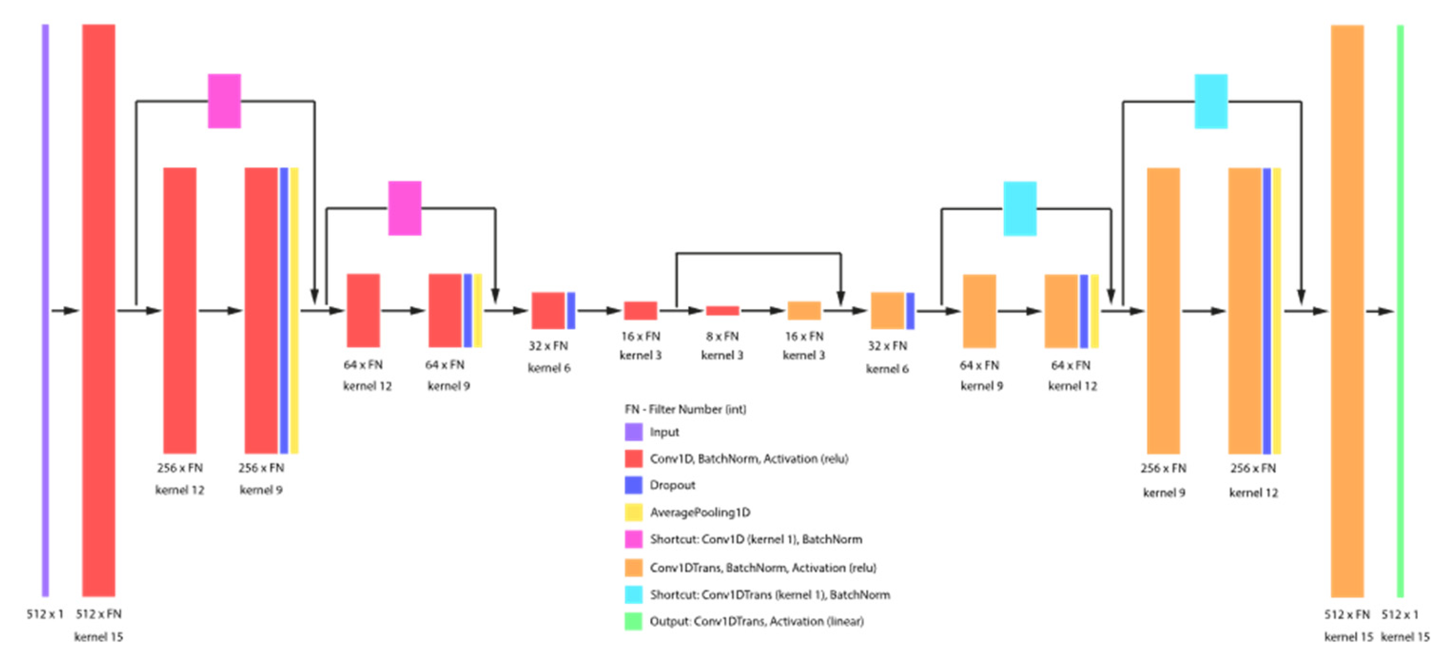
Figure 2.
Apply Model procedure schema.
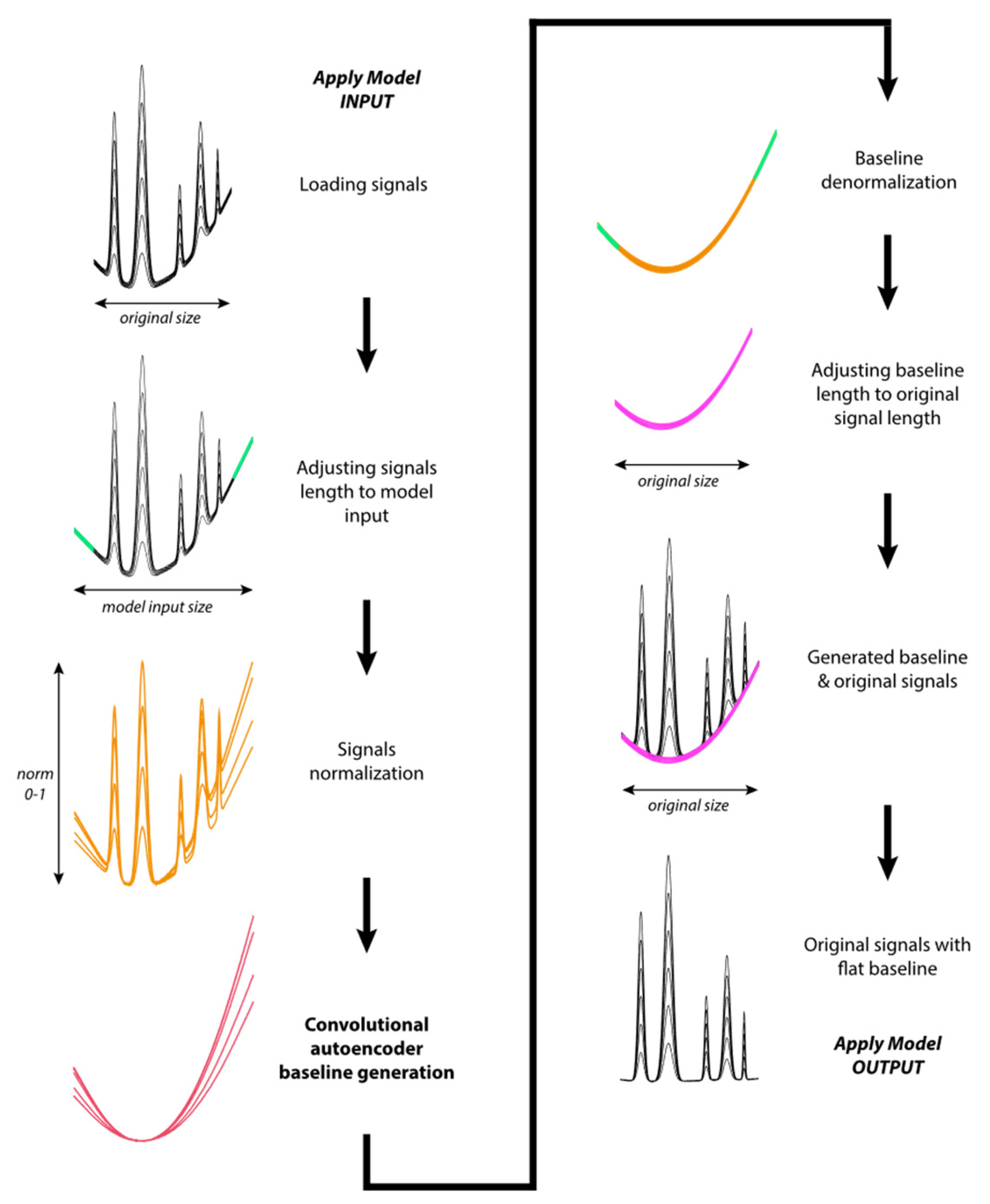
Figure 3.
Generation of simulated signals procedure.
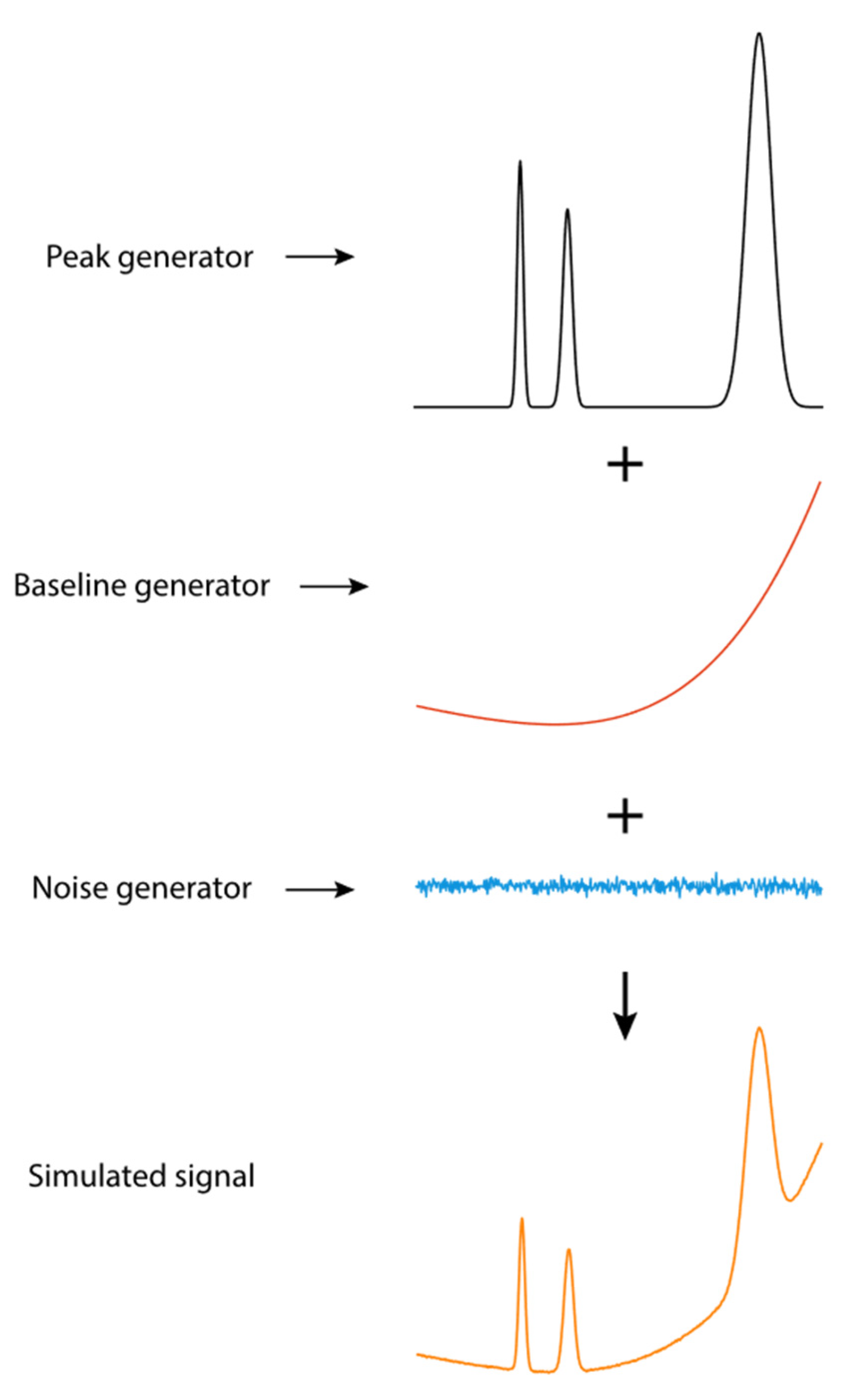
Figure 4.
Alterations in losses and learning rate during the training process of the ConvAuto model.
Figure 4.
Alterations in losses and learning rate during the training process of the ConvAuto model.
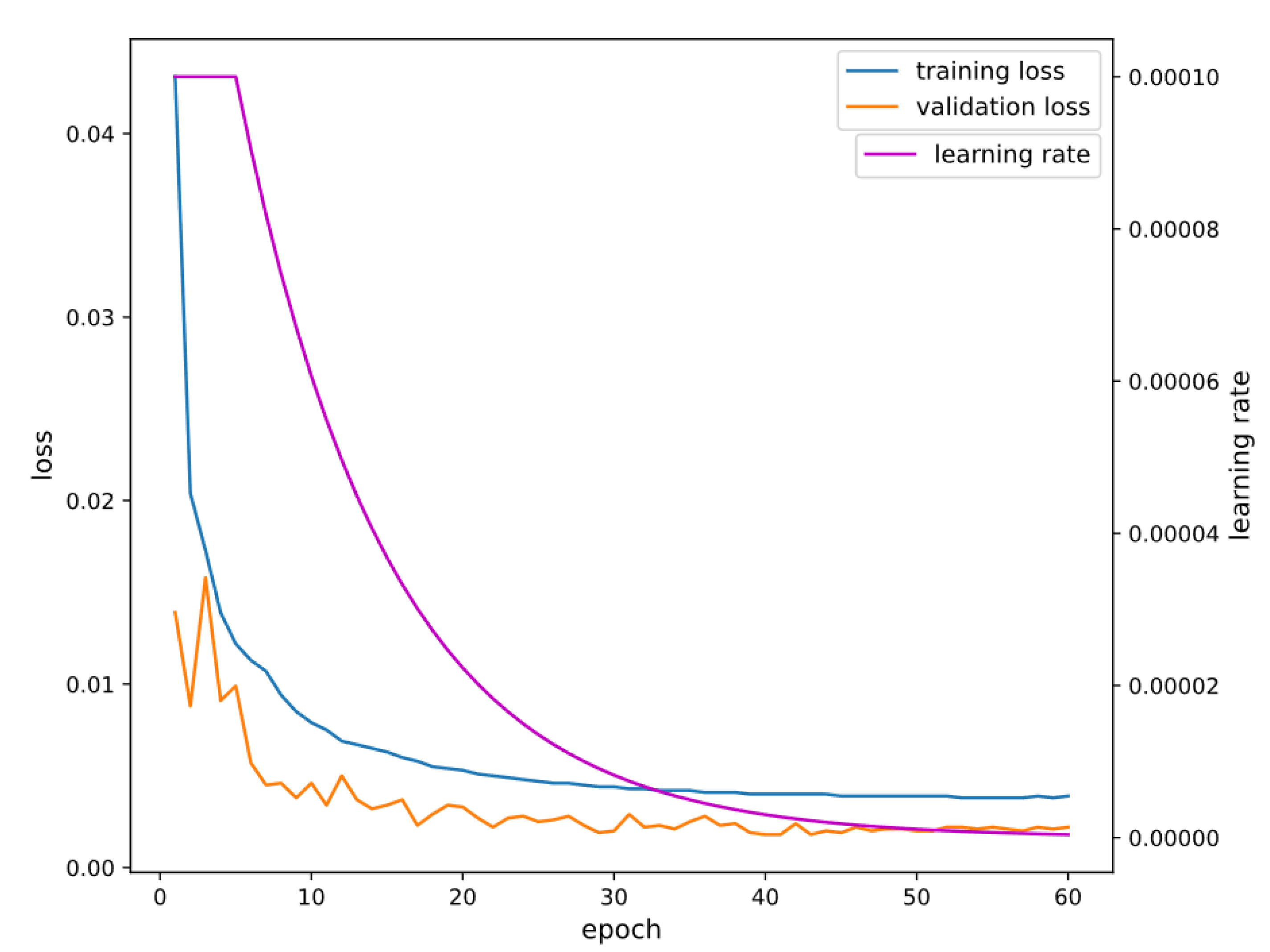
Figure 5.
Implementation of the ConvAuto model to the divers simulated sets of signals: A) SimSet 1 with 200 signal points, B) SimSet 2 with 2000 signal points, C) SimSet 3 with 2500 signal points and D) Simset 4 with 4000 signal points, respectively.
Figure 5.
Implementation of the ConvAuto model to the divers simulated sets of signals: A) SimSet 1 with 200 signal points, B) SimSet 2 with 2000 signal points, C) SimSet 3 with 2500 signal points and D) Simset 4 with 4000 signal points, respectively.
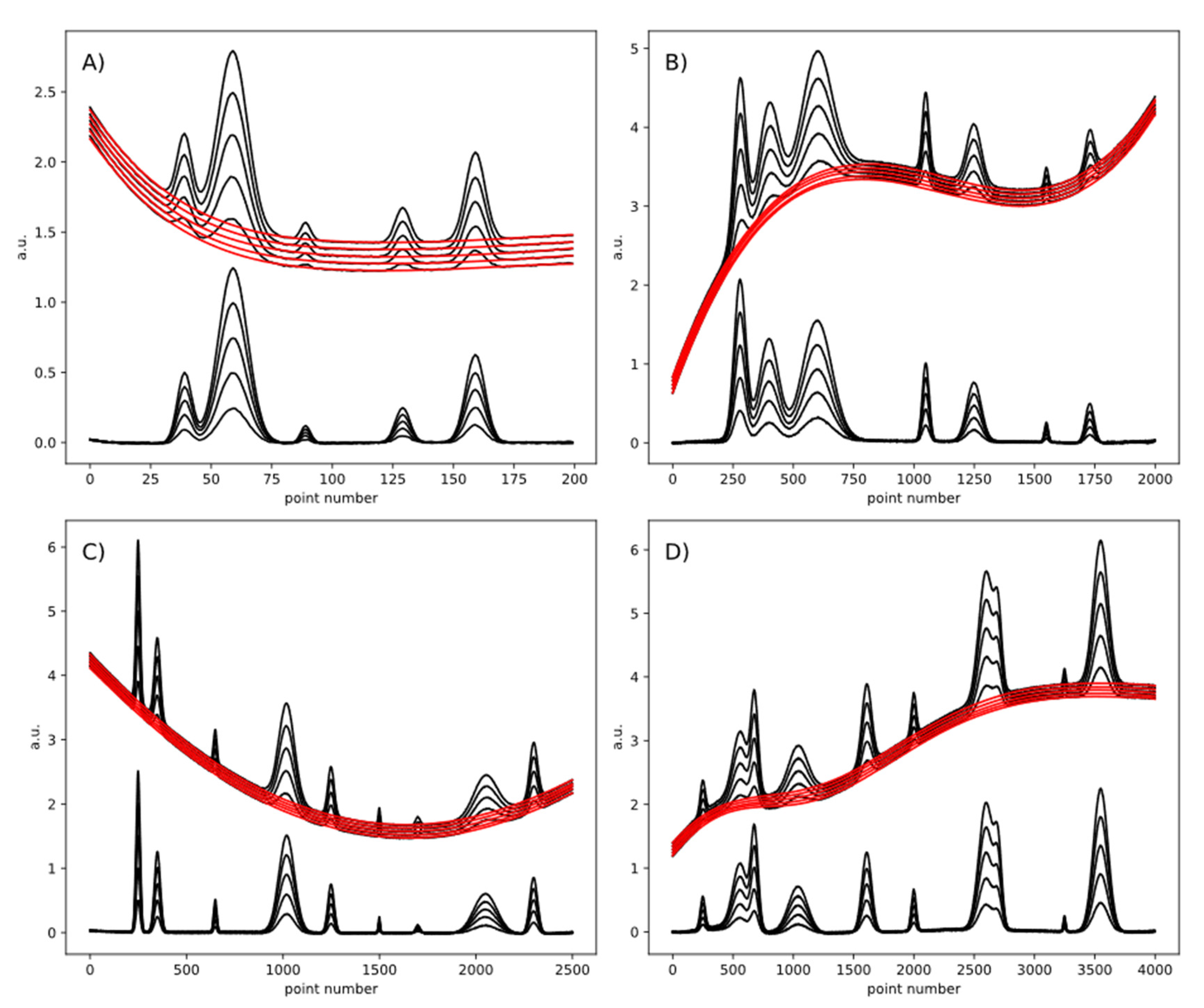
Figure 6.
Comparison of the baseline produced by the ConvAuto and ResUNet model.
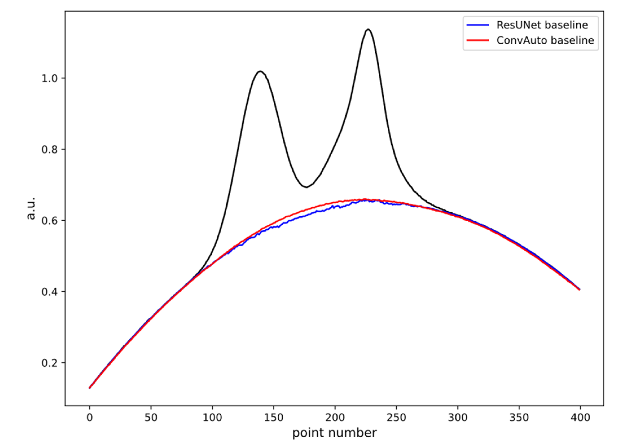
Figure 7.
The ConvAuto baseline generation for voltametric experimental signals pertaining to: A) CRM 25.0 ± 0.1 µg.l-1 Pb(II) signals with additions of 0.75, 1.50, 2.25, 3.00 µg.l-1 Pb(II) and B) ferulic, syringic, vanillic acid signals in concentration rage 1.15 – 5.80, 0.60 – 3.00, 0.50 – 2.50 mg.l-1, respectively.
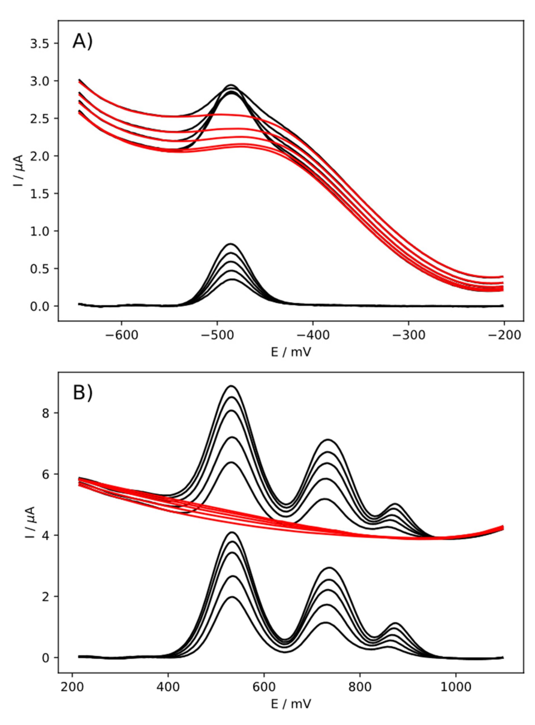
Figure 8.
Problems with ConvAuto baseline generation: A) noisy or B) underfitted fragments.
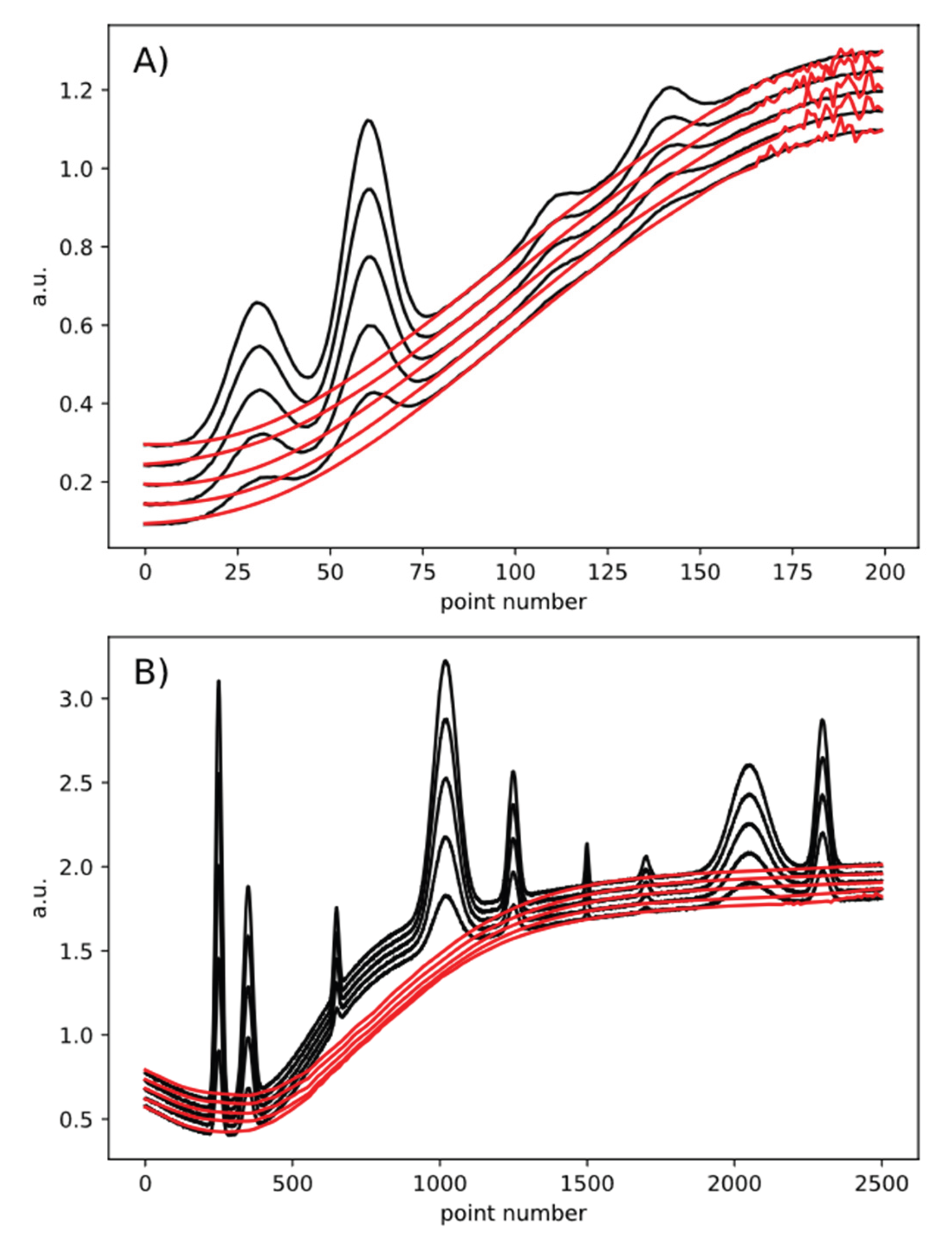

Table 1.
ConvAuto model training results.
| Loss (MAE) | Metrics (RMSE) | |
|---|---|---|
| Train | 0.0039 | 0.0093 |
| Validate | 0.0022 | 0.0047 |
| Test | 0.0022 | 0.0051 |
Table 2.
The results of the ConvAuto model application and comparison with the ResUNet model for 4 simulated sets of signals.
Table 2.
The results of the ConvAuto model application and comparison with the ResUNet model for 4 simulated sets of signals.
| ConvAuto | ResUNet | |||
|---|---|---|---|---|
| MAE | RMSE | MAE | RMSE | |
| SimSet 1 | 0.0034 | 0.0045 | 0.0023 | 0.0030 |
| SimSet 2 | 0.0192 | 0.0230 | 0.0114 | 0.0198 |
| SimSet 3 | 0.0102 | 0.0120 | 0.0119 | 0.0224 |
| SimSet 4 | 0.0198 | 0.0263 | 1.6839 | 1.7957 |
Disclaimer/Publisher’s Note: The statements, opinions and data contained in all publications are solely those of the individual author(s) and contributor(s) and not of MDPI and/or the editor(s). MDPI and/or the editor(s) disclaim responsibility for any injury to people or property resulting from any ideas, methods, instructions or products referred to in the content. |
© 2025 by the authors. Licensee MDPI, Basel, Switzerland. This article is an open access article distributed under the terms and conditions of the Creative Commons Attribution (CC BY) license (http://creativecommons.org/licenses/by/4.0/).
Copyright: This open access article is published under a Creative Commons CC BY 4.0 license, which permit the free download, distribution, and reuse, provided that the author and preprint are cited in any reuse.


