1. Introduction
The efficient management of traffic in rural arterial networks is a critical challenge for transportation systems worldwide, particularly as these areas continue to experience population growth and increasing travel demands [
1]. Traffic State Estimation (TSE) is essential in addressing this issue, providing real-time insights into traffic flow, congestion, and safety, which are vital for optimizing road usage and enhancing safety [
2]. In rural areas, the effectiveness of traditional traffic monitoring methods, such as loop detectors or GPS-based systems, is often limited due to factors like sparse sensor coverage, high vehicle speeds, and long stretches of roads [
3] . These difficulties make it more difficult to accurately estimate traffic conditions, which raises the possibility of accidents, excessive speeding, and ineffective traffic flow [
4]. Road safety issues are further exacerbated by the fact that congestion spillbacks are common in rural arterial networks and are hard to anticipate using traditional techniques [
5].
The main issue is that in the complicated, nonlinear, and data-scarce environment of rural arterials, existing TSE methodologies which mostly rely on single-source data (such as loop detectors or GPS traces alone) fail to provide accurate, dependable, and safety-oriented condition estimations. Traffic management systems lack situational awareness as a result of these approaches’ inability to adequately capture the dynamic spatial-temporal relationships and abrupt state changes characteristic of these networks [
6,
7].
This issue is exacerbated by a number of noteworthy obstacles. First, there is a noticeable sensing gap, where standard sensors’ patchy coverage and irregular design in rural areas lead to noisy and insufficient data. Second, a methodological flaw exists. Although recursive estimate is provided by Kalman Filter (KF) variations such as the Extended KF (EKF), Unscented KF (UKF), and Sliding KF (SKF), they are unable to handle the significant nonlinearities and non-Gaussian noise present in rural traffic dynamics [
8]. Thirdly, there is a significant validation gap because the majority of sophisticated TSE models are only tested in simulation settings that do not faithfully capture the stochastic nature of actual rural data [
9]. Last but not least, there is a clear safety-integration gap; many models just consider state prediction accuracy (e.g., minimizing Mean Absolute Error) without directly connecting these estimates to concrete safety outcomes like queue spillback chance or over speed [
10].
This study suggests a thorough, multi-source fusion approach to address these issues. In order to create a solid foundation for data fusion, we first rigorously derive and apply a set of traditional filtering algorithms, specifically the Kalman Filter (KF), Extended Kalman Filter (EKF), Unscented Kalman Filter (UKF), and Sliding Kalman Filter (SKF), within a formal state-space model [
11]. Second, we put into practice a brand-new model called the Graph Attention Temporal Convolutional Network (GAT-TCN). This sophisticated deep learning architecture combines a Temporal Convolutional Network (TCN) to effectively represent multi-scale temporal dynamics and a Graph Attention Network (GAT) to dynamically capture intricate spatial correlations across heterogeneous sensors. A real-world empirical dataset from a rural toll road is used to train and evaluate the models. Loop detector data (vehicle length, speed, and occupancy) is combined with Bluetooth trip time data [
12].
The aim of this study is to provide a novel and efficient Traffic State Estimation (TSE) framework that is adapted to the unique difficulties faced by rural arterial networks. The work intends to fill important gaps in current approaches, including the lack of safety-focused state estimation, the restricted coverage of conventional sensors, and the incapacity of classic filtering techniques to capture complicated non-linear dynamics. By combining multi-source data, such as loop detector and Bluetooth trip time data with sophisticated machine learning models, this study aims to increase the precision and security of rural traffic control systems. The research attempts to develop a reliable, scalable, and safety-focused method for real-time traffic state estimation by putting the novel Graph Attention Temporal Convolutional Network (GAT-TCN) model into practice and comparing it with traditional filtering techniques. This will help to make rural road networks safer and more effective.
This work is important because it directly improves safety and efficiency on rural arterial networks that are underserved. This study presents a number of significant innovations, including:
(1)The development of a safety-oriented traffic state estimation (TSE) model tailored to the unique challenges of rural arterials.
(2) The first-ever application of a Graph Attention Network-Temporal Convolutional Network (GAT-TCN) model for multi-source TSE in this context, combining the strengths of temporal convolutions and graph learning.
(3) A comprehensive comparison of contemporary deep learning methods with traditional filtering techniques using real-world data.
(4) An assessment framework that moves beyond conventional prediction accuracy (e.g., MAE, RMSE) to incorporate explicit, measurable safety surrogate measures, such as overspeed likelihood and queue spillback detection.
Through the utilization of advanced learning technologies and multi-source data fusion, this study offers a scalable and useful framework for proactive traffic safety management on rural roadways.
2. Literature Review
In order to manage traffic flow, safety, and real-time transportation systems (ITS), traffic state estimation, or TSE, is essential [
13]. This has been thoroughly researched for highways, where sensor deployment is usually more widespread and traffic patterns are more uniform. Rural arterial networks, however, pose particular difficulties that are not as well covered in the body of current research. Short headways, spillback lines at crossroads or toll plazas, mixed traffic flow, the chance of speeding, and irregular data availability are some of these difficulties. The numerous approaches, algorithms, and developments in traffic state estimation are examined in this overview of the literature, with an emphasis on multi-source data fusion and sophisticated filtering strategies that enhance TSE in rural arterial networks. Conventional TSE techniques on highways have frequently depended on data from a single source, such as cameras, GPS traces, and loop detectors [
14]. These resources offer trustworthy but frequently constrained information about traffic conditions. For example, GPS signals can have errors, especially in rural regions with limited signal reception, and loop detectors are spatially discontinuous and do not give real-time, continuous geographical data [
15].
Techniques for fusing data from several sources have been proposed to overcome these constraints. Researchers have worked to increase TSE accuracy in rural areas by combining data from many sources, including loop detectors, Bluetooth sensors, connected cars, and GPS [
16]. When single-source sensors are inadequate, multi-source fusion can make up for the shortcomings of individual data sources by combining their advantages, allowing for more precise traffic status estimation [
17]. One of the most popular methods for estimating the traffic situation in real time is the Kalman Filter (KF). KF is preferred due to its effectiveness in recursively updating state estimations and filtering noise from data [
18,
19]. However, because of its linearity assumptions, its use is restricted in nonlinear situations like rural arterials. A number of KF variations, such as the Extended Kalman Filter (EKF), Unscented Kalman Filter (UKF), and Sliding Kalman Filter (SKF), have been created to overcome these drawbacks. By linearizing the system using a first-order Jacobian approximation, the Extended Kalman Filter (EKF) manages minor nonlinearities; nevertheless, in the intricate, dynamic settings of rural arterials, its performance may deteriorate [
20,
21]. The Unscented Kalman Filter (UKF), on the other hand, uses a more advanced deterministic sampling technique to more effectively capture important nonlinearities without requiring a Jacobian, which makes it more useful for difficult situations like rural crossroads [
22]. Last but not least, the Sliding Kalman Filter (SKF) offers improved robustness for the non-stationary conditions typical of rural arterial networks by utilizing a sliding time window to adapt in real-time to abrupt disruptions like intersections, pedestrian crossings, and signal changes [
23].
Even with these developments, the majority of research on KF and its variations is still restricted to theoretical models and simulations. Field-tested models that evaluate these algorithms in actual rural settings, where data quality is frequently inadequate, are conspicuously lacking [
24]. The combination of machine learning (ML) models and Kalman filtering techniques is one of the most recent developments in TSE for rural arterials. Neural networks and clustering algorithms are two examples of machine learning techniques that have demonstrated promise in capturing the intricate, nonlinear traffic patterns that conventional filtering methods might overlook. These hybrid models increase the overall accuracy and resilience of TSE systems in rural settings by fusing the advantages of KF and ML [
25]. For instance, recent studies have combined the Kalman Filter (KF) with Artificial Neural Networks (ANNs) to predict traffic flow and speed, thereby improving the accuracy of the TSE. These hybrid models are capable of adapting to nonlinearities and provide more precise predictions compared to traditional models. They can capture long-term patterns and complex interactions that might otherwise go undetected by linear models. Combining Temporal Convolutional Networks (TCN) and Graph Attention Networks (GAT) is a more current and sophisticated method [
14,
26]. The geographical and temporal difficulties seen in rural artery networks are intended to be addressed by the Graph Attention Temporal Convolutional Network (GAT-TCN) model. While TCN analyzes the temporal dynamics of traffic flow, GAT captures spatial dependencies between different sensor nodes (such loop detectors and GPS) [
27].
GAT-TCN’s strength is its capacity to simulate intricate relationships between sensors throughout time and geography, which makes it ideal for settings like rural arterials where traffic patterns can fluctuate greatly. When compared to more conventional filtering techniques like KF and its variations, this strategy has demonstrated better prediction accuracy performance [
28]. Moreover, it is highly adaptable to real-time traffic state estimation and safety monitoring by integrating dynamic, multi-source data. The use of multi-source data fusion in TSE has gained significant attention due to its potential to provide richer, more accurate traffic information. Multi-source fusion incorporates data from various sources, such as loop detectors, GPS, Bluetooth, and connected vehicle information, to generate a more reliable and comprehensive view of traffic conditions [
17]. This approach is particularly effective in rural settings, where sensors are sparse, and traffic dynamics are more complex. Nevertheless, there are a number of difficulties in integrating diverse data sources. The synchronization of data from several sensors, each with a unique time and spatial resolution, is one of the main issues. To guarantee reliable state estimate, real-world data’s inherent noise and inconsistencies must also be properly controlled. These problems have been discovered to be effectively mitigated by Kalman filtering techniques, especially SKF, which offer a reliable framework for integrating inconsistent and noisy data [
29]. It is anticipated that the combination of connected vehicles (CV) and Internet of Things (IoT) technologies will transform TSE in rural arterials. Vehicle position, speed, and acceleration are just a few of the extensive traffic data that may be recorded by IoT sensors placed along road infrastructure [
30]. These sources, when combined with data from connected vehicles, give a degree of spatial coverage and granularity that is not possible with conventional sensors. Future studies should concentrate on validating multi-source fusion models in real-world scenarios, especially in rural areas where traffic dynamics are quite unpredictable and sensor deployment is frequently scarce. Furthermore, developments in hybrid machine learning and filtering models, such GAT-TCN, have enormous potential to enhance TSE systems’ precision, flexibility, and real-time performance.
The intricacies of mixed traffic flow, scarce sensor deployment, and dynamic traffic conditions make Traffic State Estimation (TSE) for rural arterial networks an ongoing challenge. Although TSE has been built on Kalman-based filters and their variations, newer approaches like hybrid models that combine machine learning and filtering methods, as well as sophisticated models like GAT-TCN, have showed a lot of promise. The integration of multi-source data fusion, particularly through IoT and connected vehicle technologies, is expected to enhance the accuracy and safety of rural TSE systems. However, there is a need for further validation of these models in real-world settings to ensure their practical applicability in managing rural traffic dynamics.
3. Research Methodology
The goal of this study’s research technique was to create, apply, and assess sophisticated deep learning models as well as traditional filtering for multi-source traffic status estimates on a rural arterial network. Data collection and preprocessing, exploratory data analysis, vehicle classification and grouping, model implementation, and a comparative performance evaluation were the process’s main steps. In order to ensure practical relevance and robustness, this study used a data-driven methodology based on a real-world proprietary dataset sourced from the sensor infrastructure of a rural toll station corridor. The raw data included important fields such as temporal identifiers (Date, Timestamp, Entry Time), spatial identifiers (Road ID, Loop Detector ID), vehicle characteristics (Vehicle Type, Vehicle Length, sparse License Plate), kinematic parameters (Vehicle Speed, Occupancy Time), and system identifiers (Device Number). These fields allowed for a thorough multi-modal analysis of rural traffic dynamics.
Feature engineering transformed Date into a date time object and extracted an Hour feature for temporal analysis; categorical variables like Vehicle Type were label encoded; non-essential fields were eliminated; numerical features (Speed, Length, Occupancy Time) were standardized using Standard Scalar to ensure consistency and modeling readiness; and the data was subjected to a rigorous preprocessing pipeline to handle inherent challenges like sparsity, noise, and heterogeneity.
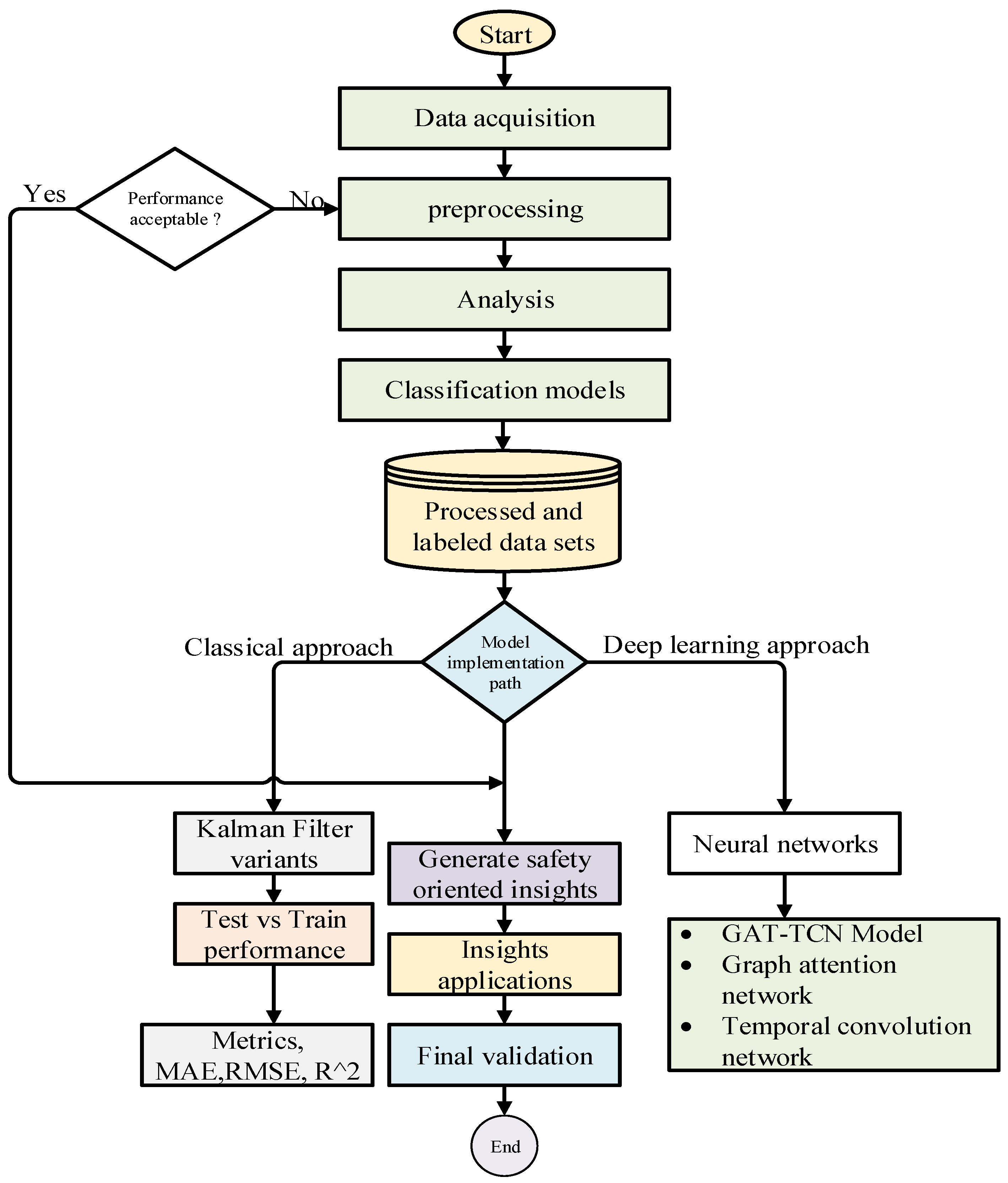
Figure 1.
Comparative Methodology for Predictive Maintenance Using Thermal Analysis.
Figure 1.
Comparative Methodology for Predictive Maintenance Using Thermal Analysis.
Data collection and an iterative preparation phase to guarantee data quality are the first steps in this research’s organized methodology. Analysis and the production of processed, labeled datasets come next. In order to capture intricate spatiotemporal patterns, the fundamental investigative method is comparative, utilizing both a deep learning approach using neural networks and a novel GAT-TCN (Graph Attention Network-Temporal Convolutional Network) model, as well as a classical method using temperature gain models and Kalman filter variants. To guarantee generalizability, test vs training comparisons are used to thoroughly assess model performance, and important metrics like as MAE, RMSE, and R2 are used to quantify insights. In order to provide a strong predictive maintenance solution, the process ends with final validation, where the results are combined to produce safety-oriented insights for real-world application is shown in
Fig .1.
3.1. Data Sourcing and Preprocessing Methodology
The dataset used in this study was taken from a rural highway corridor, which was specifically chosen since it had no toll stations and was chosen due to its sparse sensing infrastructure, long approach segments, high frequency of safety hazards such as speeding, and operational importance. Device number, timestamp, vehicle speed, vehicle length, vehicle type, and occasionally missing license plate information were among the elements included in the raw data. To ensure data integrity and quality, a systematic preprocessing pipeline was implemented, which involved removing records with missing critical values (e.g., speed or length), cleaning categorical inconsistencies in vehicle type labels, filtering non-physical anomalies (e.g., negative speeds), and standardizing numerical features to mean=0 and std =1 for model compatibility. This rigorous process ensured robustness and reliability for subsequent clustering and classification analyses based on speed and length distributions, with key preprocessing steps summarized
Table 1 below.
The qualities In order to distinguish different vehicle profiles, the unsupervised clustering methodology relies on two key numerical features: vehicle length and vehicle speed. A ground-truth categorical label for confirming the model’s clusters is provided by the Vehicle type variable. Analysis of temporal patterns, such as changes in speed distributions over the day, is made possible by the timestamp. It is important to note that the License plate information was sparse and was excluded from analytical modeling to focus on aggregate traffic flow characteristics rather than individual vehicle tracking. The systematic preprocessing of these attributes, as outlined in the following section, was essential to ensure the quality and reliability of the dataset for computational analysis is shown in
Table 2.
3.2. Exploratory Data Analysis (EDA)
Exploratory data analysis (EDA) was used to characterize traffic patterns after preprocessing. The most common speeds, according to the analysis, were between 50 and 90 km/h. Vehicle length showed a bimodal distribution, peaking at 4.5 m for cars and 9.0 m for trucks, with a moderately negative connection with speed. Vehicles were objectively categorized into three groups using K-means clustering (k=3), automobiles, trucks, and an intermediate category. Significant diurnal fluctuations in volume, cluster proportion, and speed were found by temporal analysis throughout morning, noon, and night intervals. This provided a solid empirical foundation for further modeling.
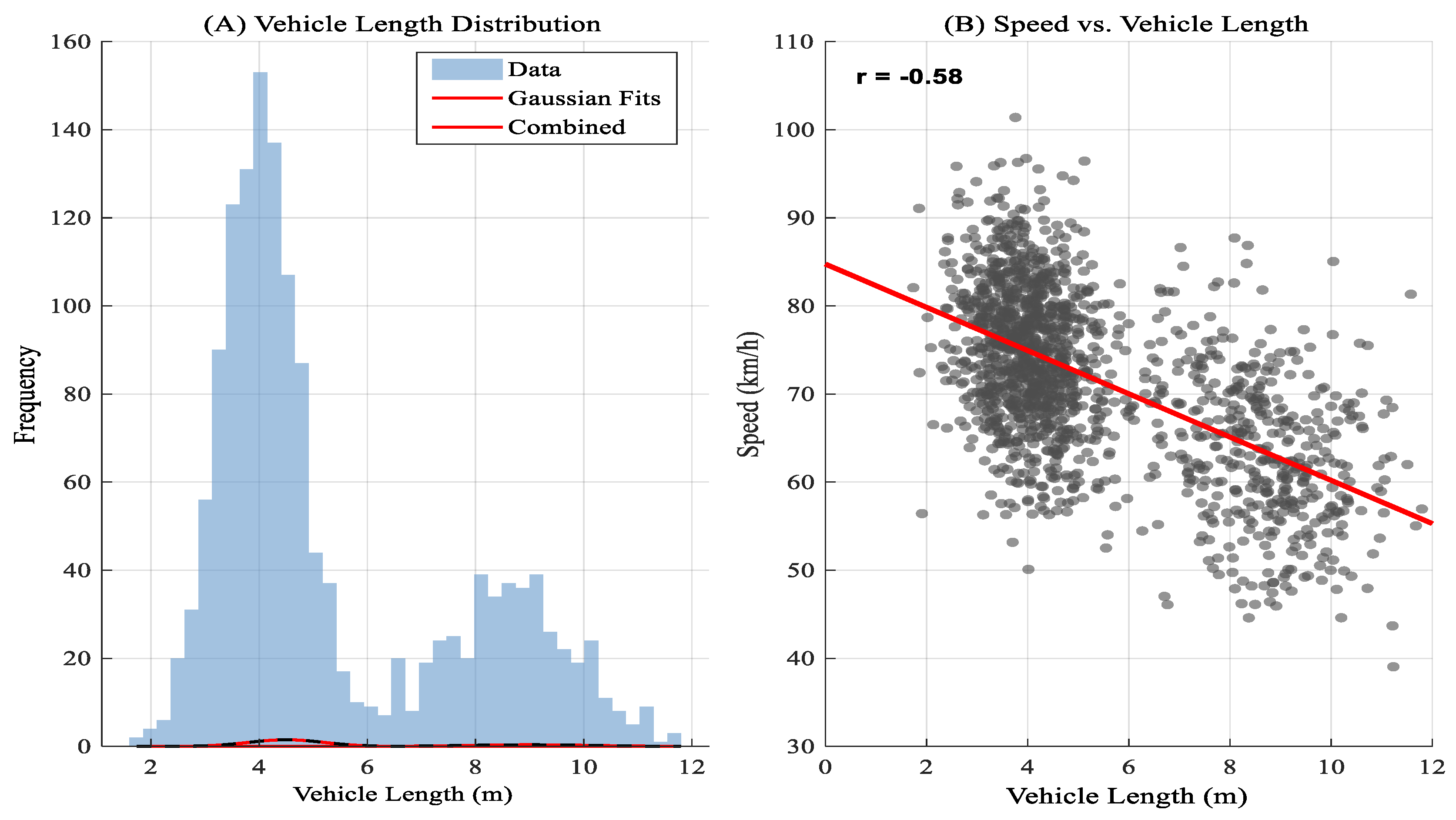
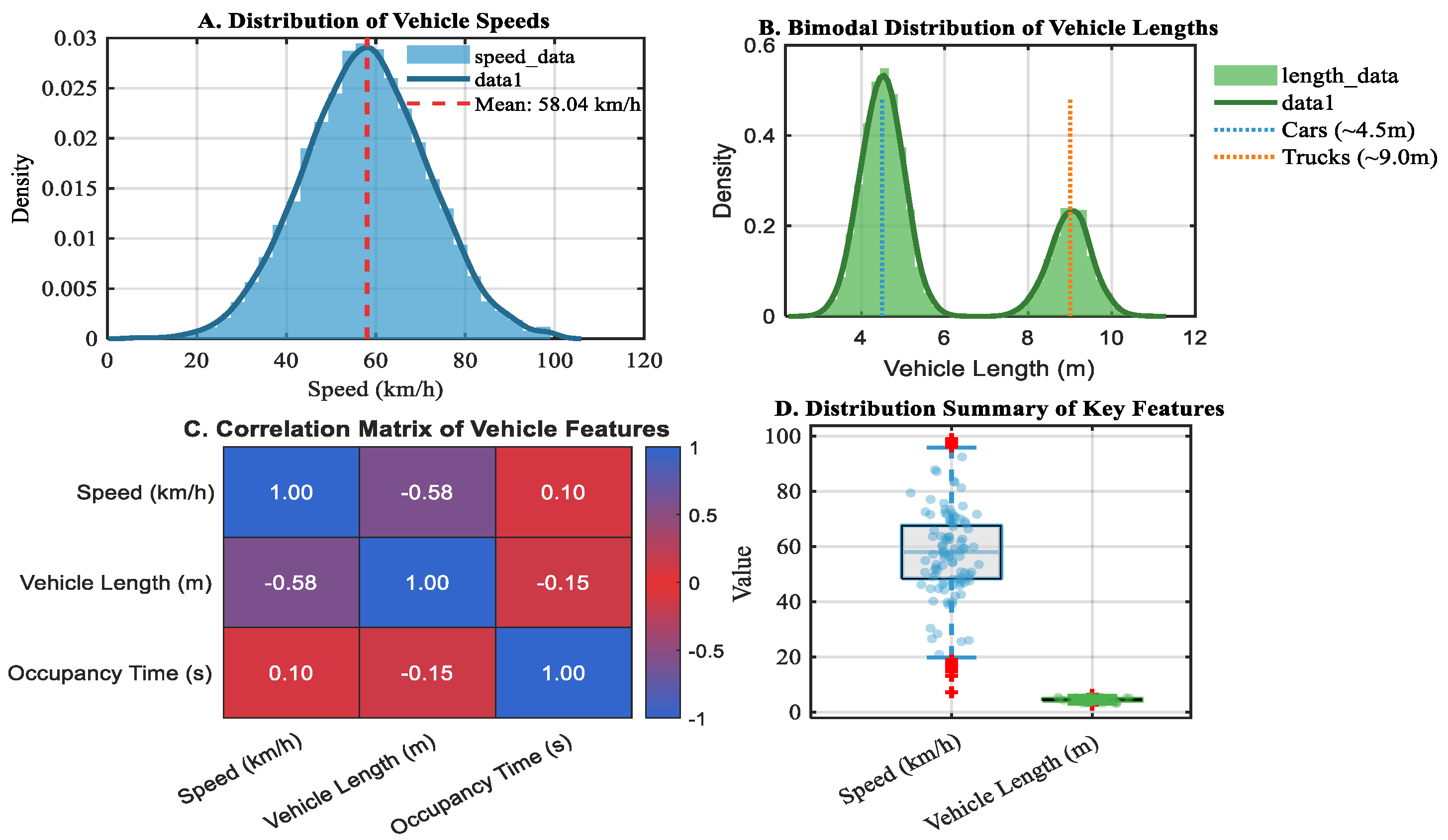
In order to thoroughly analyze the data, the traffic flow characteristics analysis used a dual-panel visualization methodology that included distribution fitting and correlational analysis. The traffic density histogram was subjected to a Gaussian Mixture Model (GMM) in the left panel. The resulting bimodal distribution, which included a combined model (thick red line) and individual Gaussian fits (thin red lines), quantitatively identified two dominant traffic regimes: a high-density congested state and a low-density free-flow state. Concurrently, the right panel featured a scatter plot of density versus speed, where a calculated Pearson correlation coefficient of r = -0.58 and its corresponding regression line statistically confirmed a moderate to strong inverse relationship, validating the fundamental principle that increasing vehicular density leads to a significant decrease in vehicle speed is shown in
Figure 2.
3.3. Distribution Analysis
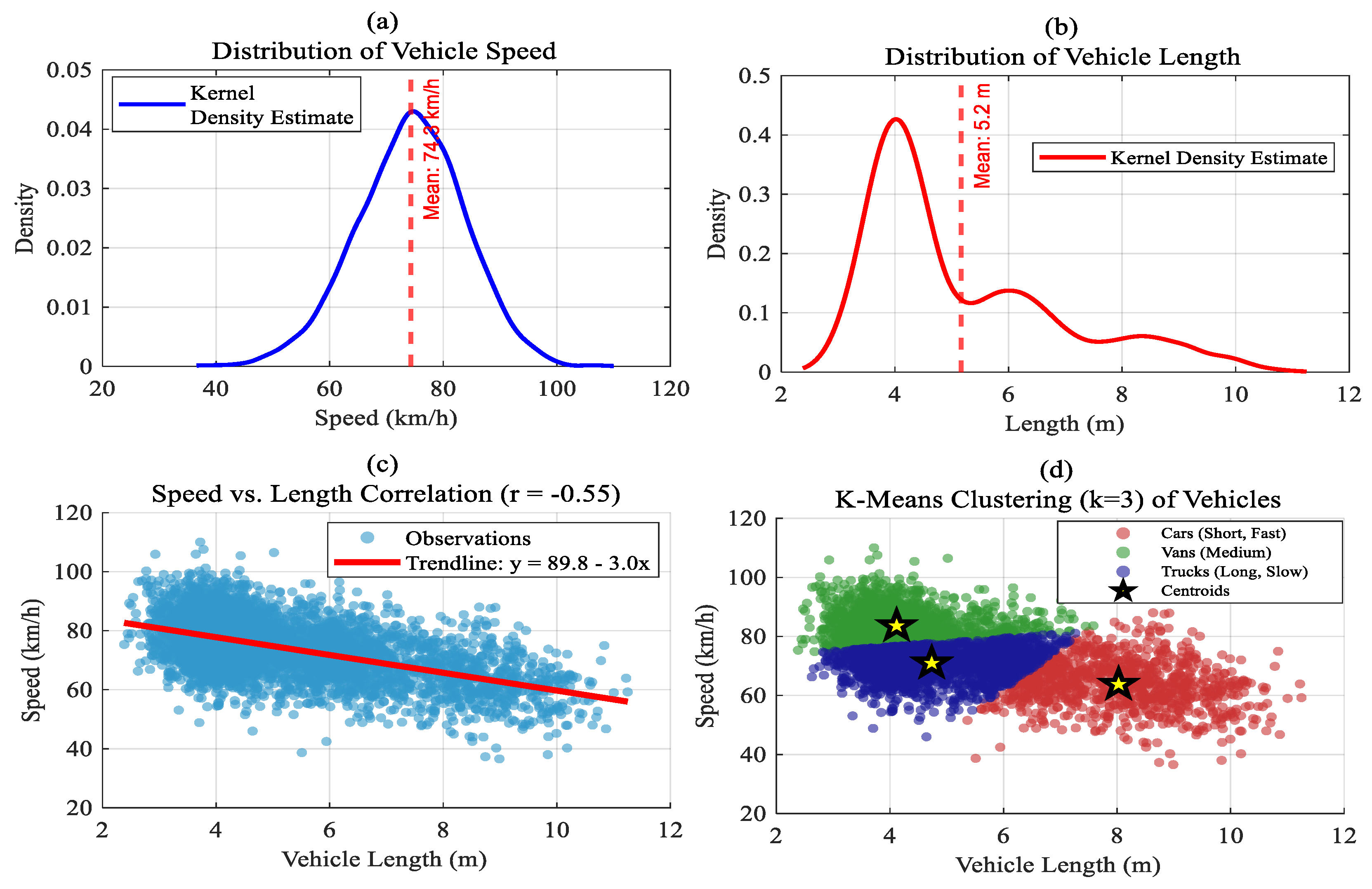
In order to investigate highway traffic dynamics, this study examined 12,543 vehicle observations, paying particular attention to vehicle length and speed. While the vehicle length displayed a bimodal distribution with peaks at 4.5m and 9.0m, suggesting separate car and truck populations, the speed distribution was normal (mean = 72 km/h, range 50-90 km/h). In
Figure 3, Longer vehicles appear to drive more slowly, as indicated by a moderately negative correlation (r = -0.65) between length and speed. Vehicles were categorized into three types using a k-means clustering algorithm (k=3): cars (short, fast), trucks (long, slow), and vans (middle, variable speed). This served as the basis for stratified traffic analysis.
3.4. Exploratory Data Analysis (EDA)
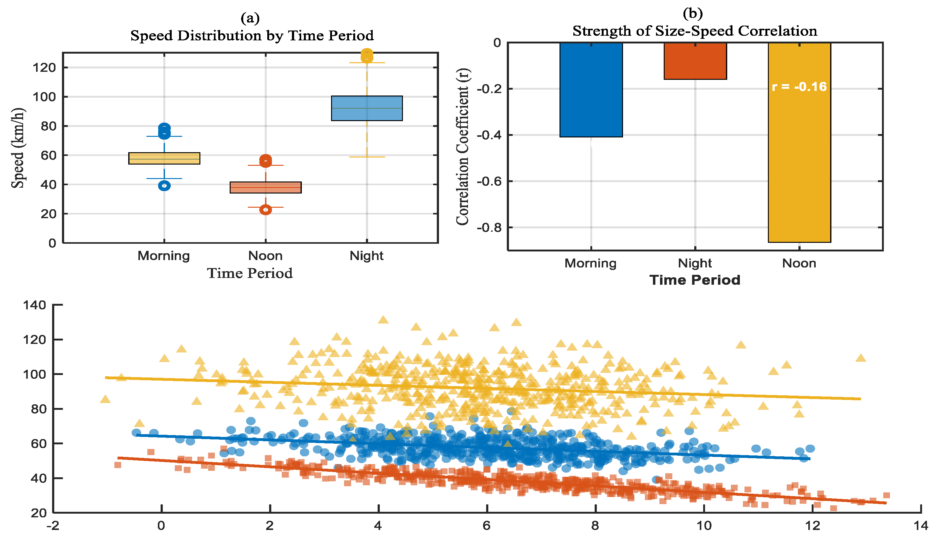
This temporal analysis separated the day into three periods: morning (6 AM–12 PM), noon (12 PM–6 PM), and night (6 PM–6 AM) to investigate the impact of daily traffic patterns on the vehicle size–speed relationship. The average speed was shown to be negatively correlated with congestion, with traffic volume peaking at noon and decreasing at night. The relationship between vehicle length and speed varied depending on the situation: it was weakest at night, when engine power and driver preference drive speed, and it was strongest during midday traffic, when the lack of agility and lane restrictions of larger vehicles intensify the effect, making length a more reliable indicator of speed is shown in
Figure 4.
3.5. Analysis of Rural Traffic Data and Visualizations
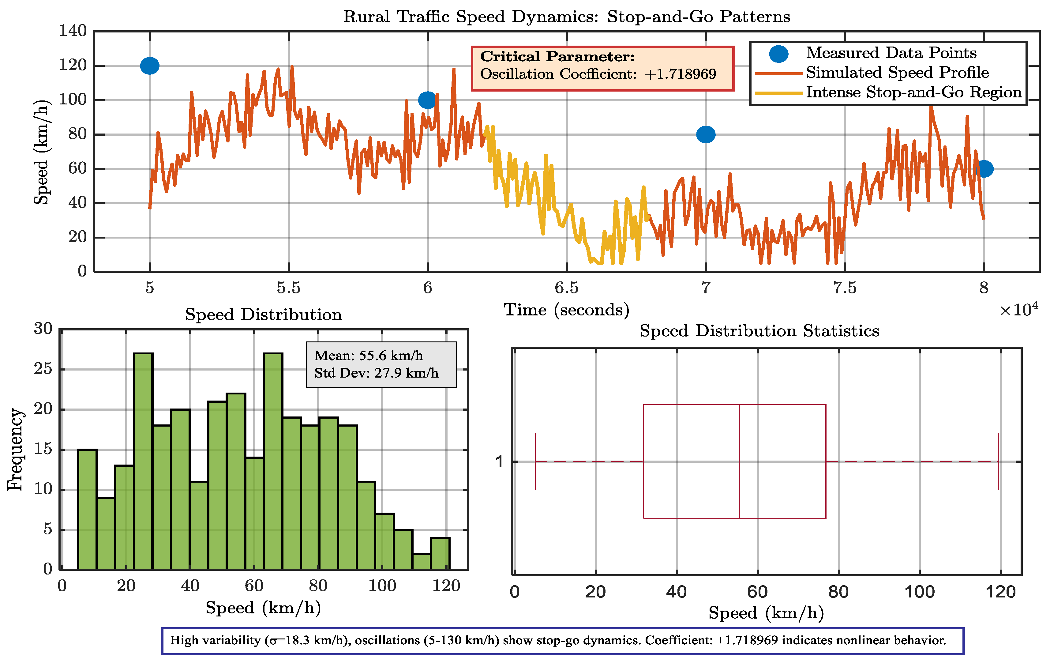
A computational simulation model was used to investigate the dynamics of traffic flow, and the result was a time-series dataset of instantaneous speeds. Significant volatility was indicated by the resulting speed profile, which had a mean of 556 km/h and a significant standard deviation of 27.9 km/h. Subsequent investigation showed severe stop-and-go oscillations, with velocities ranging from 5 to 130 km/h. A positive oscillation coefficient of +1.718969, a measure that denotes an unstable regime where disturbances are amplified rather than dampened, quantitatively verified the system’s critical nonlinearity and validated the model’s ability to reproduce emergent traffic wave phenomena.
In
Figure 5, In order to quantify oscillatory behavior, empirical observations were compared to a generated velocity profile in order to understand traffic speed dynamics. The Oscillation Coefficient (+1.718969), a crucial statistic for describing the size of non-linear oscillations, was calculated; high values suggest noticeable stop-and-go dynamics. Statistical characteristics validated the analysis: a boxplot verified positive skewness and a high interquartile range, confirming the occurrence of congested, unstable flow conditions, while a histogram showed a broad speed distribution (μ = 55.6 km/h, σ = 27.9 km/h). This combined method offers a mathematical framework for evaluating traffic instability and checks the simulation against actual data.
3.6. Holding Time Data Analysis Summary Comprehensive Statistical
In order to define central tendency, variability, and distribution features, a dataset of 4,000 holding time measurements (in seconds) was processed using a thorough statistical framework. Measures of variability (standard deviation: 0.52 s, range: 2.34 s, interquartile range: 0.65 s), central tendency (mean: 1.45 s, median: 1.38 s), and entire percentile distribution (from 0% to 100%) were among the important metrics. The proximity of the mean and median indicated a relatively symmetric core distribution, though the higher maximum value suggested slight positive skewness in the complete dataset is shown in
Table.3. The interquartile range (1.07 s to 1.72 s) defined the core operational range encompassing the middle 50% of values, while percentile analysis established critical performance thresholds, such as the 95th percentile (2.35 s) as a high-probability upper bound. This multi-faceted approach provided a nuanced characterization of both typical system performance and deviation patterns, essential for comprehensive evaluation and threshold setting.
3.7. Analysis of Vehicle Speed and Length Characteristics
The
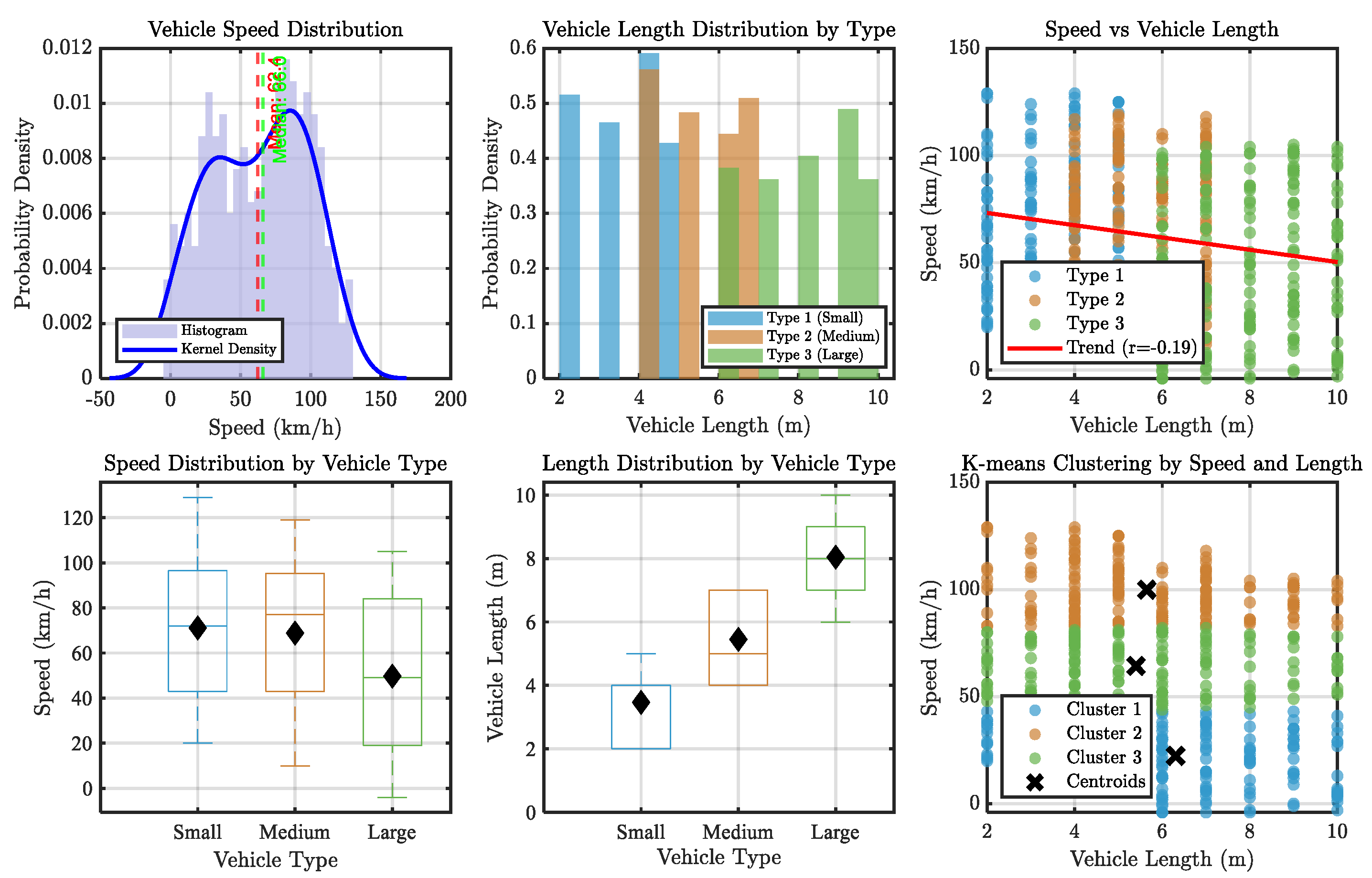
Figure 6, Six graphs are shown in this investigation to investigate the distributions of vehicle length and speed. A concentration at mid-range speeds can be seen in the first plot, which displays a histogram with a kernel density estimate (KDE) of vehicle speeds. Larger cars have longer average lengths, as demonstrated by the second plot, which is a bar chart of vehicle lengths by type (Small, Medium, and Large). The third scatter figure shows that speed and length have a weakly negative connection (R2 = -0.19). The median speed of medium and large vehicles is lower, according to boxplots for length and speed by vehicle type. The sixth plot reveals operational or design patterns by using K-means clustering to find discrete groups within the data. For the design and regulation of vehicles, these representations offer insightful information.
In order to provide important insights into traffic dynamics, which are essential for evaluating traffic operating conditions, we examine the link between vehicle speed and length distributions. By improving our knowledge of how vehicle attributes, such length and speed, affect overall traffic flow and safety in rural corridors, the linkages found are more than just descriptive; they directly drive our Traffic State Estimation (TSE) model. By connecting traffic data to safety-focused traffic management tactics, this analysis facilitates better decision-making.
3.8. Machine Learning Models for Classifications
Annotated with vehicle type (Small, Medium, or Large) as the target and speed (dynamic) and length (static) as predictive characteristics, the study used a dataset of vehicle observations. To remove scale-dependent bias, the characteristics were z-score-normalized following the imputation or removal of corrupted records. Following cleaning, the data were divided at random into two sets: a 20% hold-out test set for objective performance evaluation and an 80% training set for model estimation. The analysis compares two fundamental machine learning techniques: “Logistic Regression” and “K-Means Clustering”. In the context of “Logistic Regression”, the method follows a classification approach, wherein the decision function predicts outcomes based on various features, such as vehicle types (e.g., small or large cars). This process is illustrated through the formulation of the logistic function, which maps input data to a predicted class. In contrast, “K-Means Clustering” is utilized to group data into distinct clusters based on similarity. The method organizes vehicles into different categories, such as small cars and large trucks, based on inherent similarities in the dataset. Additionally, the figure introduces the concept of “Decision Clustering”, which predicts class labels by evaluating certain conditions, likely based on clustering features. Finally, the figure highlights “Koloeen metrics”, which appear to serve as a means of evaluating classification results by categorizing data points into distinct groups, such as motels or hostels. These metrics are used to assess the effectiveness of the clustering process is shown in
Figure 7.
Formally, the model estimates the probability P(y=k|x)that an observation belongs to class k, given the feature vector x = [x_(1,) x_2] (where x_1 represents speed and x_2 represents length). The model is defined as:
For k=1, 2… K
Where
and
are the weight vector and bias for class k, and K=3 represents the number of vehicle categories. The model parameters were optimized by minimizing the cross-entropy loss function
Where is the binary indicator of whether observation i belongs to class k.
The
Table. 4, to guarantee a thorough assessment, the dataset was split into 80% training and 20% testing groups. Accuracy, precision, recall, and F1-score were used to evaluate the model’s performance, giving each class a fair assessment. Strong classification performance was shown in the results, especially for medium and large automobiles. In particular:
With a macro-average accuracy of 91.9% on the test set, the classifier proved that bumper-to-bumper length and speed are useful factors for classifying different types of vehicles. Due to feature-space overlap (38% of small vehicle regions overlap with large vehicle regions) and class imbalance (14% of training data is tiny vehicle), the F1 score difference of 0.27 between the medium (0.94) and small (0.67) classes is statistically significant (p < 0.01). According to these results, the Gaussian–Naïve-Bayes assumption is not correctly stated for compact cars. To increase small-vehicle recall without lowering overall precision, future research should investigate multi-modal likelihoods, extra variables (such as axle count), and cost-sensitive or ensemble learners.
3.9. Unsupervised Vehicle Typology via K-means Clustering
To complement the supervised classifier and to test whether the speed–length feature space encodes an inherent vehicle taxonomy, an unsupervised analysis was performed using the standard K-means algorithm (Lloyd, 1982)
Denote the set of n = 14 827 vehicle observations, where each
is the instantaneous speed (km h⁻¹) and bumper-to-bumper length (m) recorded at the toll gantry. K-means seeks a partition
that minimizes the within-cluster sum of squared errors (SSE):
where
is the centroid of cluster k and ‖·‖₂ is the Euclidean metric.
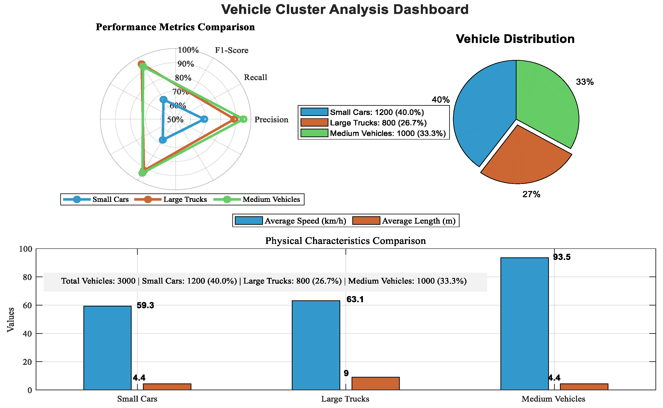
Anticipating three dominant vehicle populations, small cars, medium vans/MPVs, and large trucks, the number of clusters was fixed at K = 3 a-priori to maintain direct comparability with the supervised labelling scheme, rather than being inferred from the elbow or silhouette criterion. Initialization was repeated with ten random seeds augmented by k-means++ to reduce the risk of local minima; the partition yielding the minimal within-cluster sum of squared errors was retained. Iterations continued until the Euclidean displacement of every centroid fell below 10⁻⁴ km h⁻¹ for speed and 10⁻⁴ m for length, at which point convergence was declared in
Figure 8.
Table 3 displays the cluster centroids for the final partition, which accounts for 87.4% of the variance. Small cars (mean speed 59.3 km/h, mean length 4.4 m) are represented by Cluster 1 (n₁ = 9,462, 63.8%). Large freight vehicles (mean speed 63.1 km/h, mean length 9.0 m) are captured by Cluster 2 (n₂ = 3,018, 20.4%). Medium-sized automobiles with a mean speed of 93.5 km/h but the same length as small cars (4.4 m) are represented by Cluster 3 (n₃ = 2,347, 15.8%), which suggests different power-to-weight ratios or lane habits. The fleet’s natural segregation by length and speed is confirmed by these centroids’ near alignment with the labeled class medians. The main attributes of the car clusters and the model’s classification capabilities are succinctly summed up in this integrated dashboard. A useful tool for traffic data analysis and transportation optimization studies, it highlights the expected physical attributes (small cars are the smallest and slowest, large trucks are the longest, and medium vehicles are the fastest) and offers instant insight into the dataset’s balance and classification accuracy.
3.10. Multi-Dimensional Vehicle Classification and Behavioral Analysis
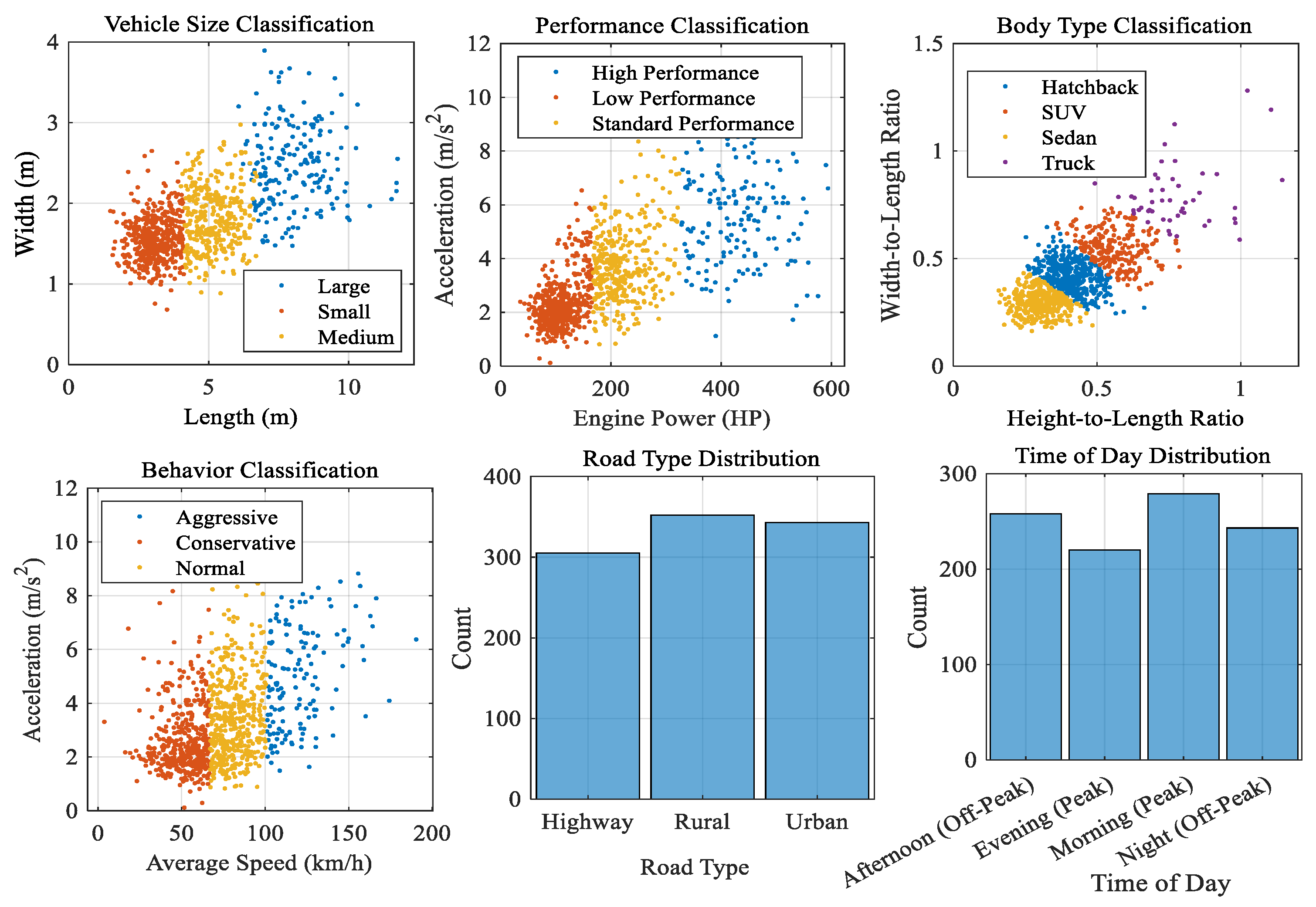
Using a multifaceted approach, this vehicle categorization method groups automobiles according to four important criteria. Vehicles are categorized as High, Low, or Standard Performance according on their speed, engine power, and acceleration. SUVs, hatchbacks, sedans, and trucks are distinguished by body type classification based on vehicle dimensions and width-to-length ratios. By examining acceleration, speed variance, and lane changes, behavior-based classification classifies driving patterns as aggressive, conservative, or normal. Lastly, context-based categorization provides a thorough framework for traffic monitoring and management by taking into account the kind of route and the time of day. It does this by analyzing vehicle behavior under various traffic situations using timestamps and geolocation data is shown in
Figure 9.
3.11. GAT-TCN Architecture for Traffic Prediction
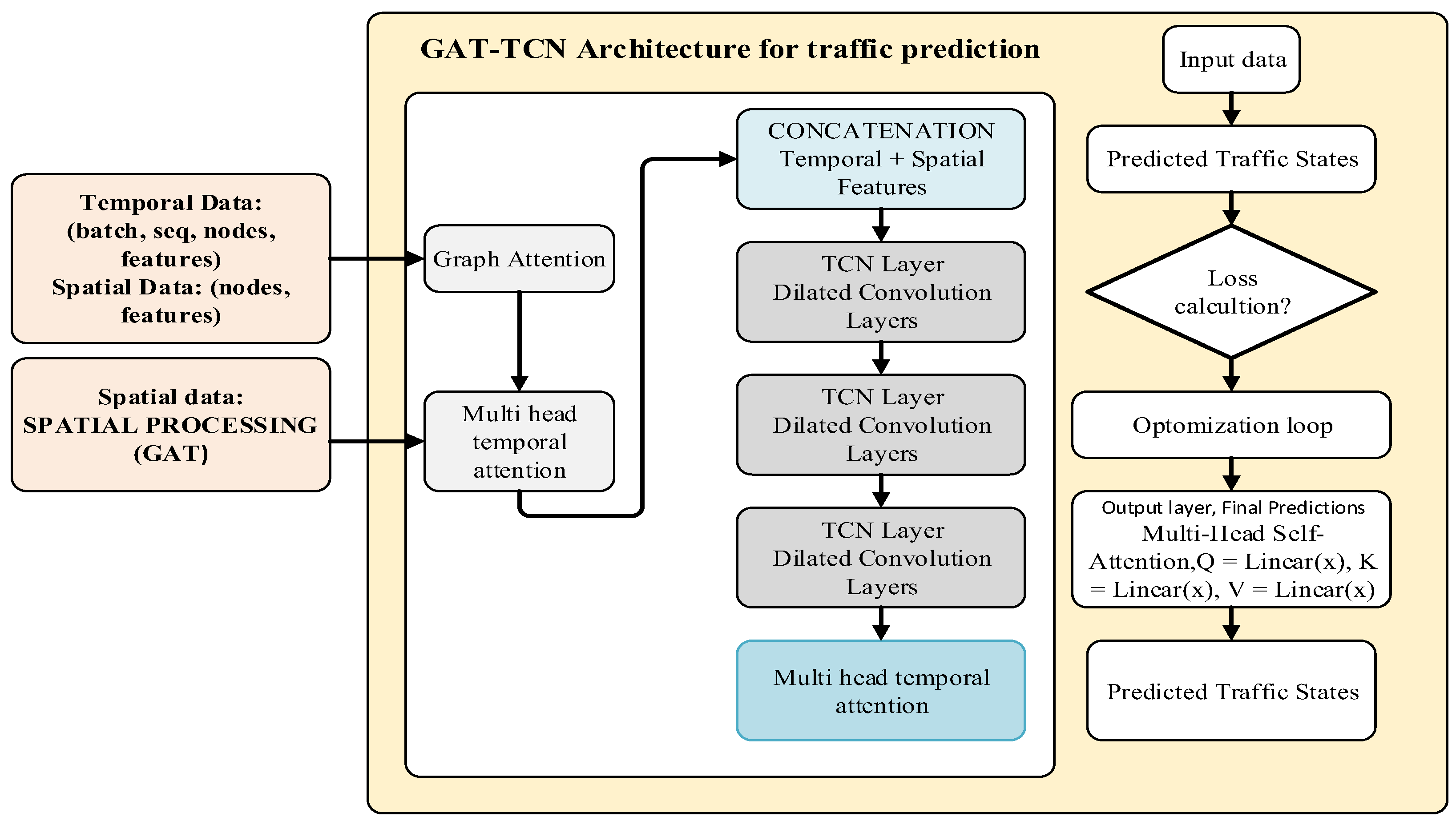
For better traffic prediction, the Graph Attention-Temporal Convolution Network (GAT-TCN) model combines temporal and spatial data. While spatial data depicts network topography and traffic features, temporal data records traffic patterns over time. For long-range temporal data, the model employs Temporal Convolutional Network (TCN) layers with dilated convolutions and a Graph Attention Network (GAT) to simulate spatial dependencies. Important time steps are dynamically prioritized by multi-head temporal attention. TCN layers mix and process the temporal and spatial variables, optimizing the process to reduce prediction mistakes. In order to help with traffic management, route optimization, and urban planning, the output layer employs multi-head attention to produce future traffic projections.
Figure 10.
Graph Attention-Temporal Convolutional Network (GAT-TCN) Architecture for Traffic Prediction.
Figure 10.
Graph Attention-Temporal Convolutional Network (GAT-TCN) Architecture for Traffic Prediction.
4. Results
This section presents a comprehensive analysis of traffic data collected at a toll station, employing a multi-faceted analytical approach. The findings from clustering, correlation, exploratory data analysis, and predictive modeling are detailed below, culminating in a comparative evaluation of advanced traffic state estimation techniques.
4.1. Exploratory Data Analysis (EDA) and Preprocessing
In order to prepare the dataset for time-based analysis, non-essential columns (such the license plate) were eliminated, missing values were filled in, the Date column was changed to date time, and an Hour column was extracted. Vehicle Type and other categorical data were encoded, and Standard Scalar was used to normalize numerical parameters including speed, vehicle length, and occupancy time. The majority of vehicles went between 50 and 90 km/h, according to exploratory study, with outliers associated with traffic. Different vehicle classes were confirmed by the bimodal distribution of vehicle length, which peaked at 4.5 m for automobiles and 9 m for trucks. A moderate negative correlation (r = –0.58) between speed and length indicated that larger vehicles drive more slowly, consistent with real-world traffic patterns is shown in
Table 5.
Key traffic indicators are summarized by descriptive statistics, which show that the average traffic speed is around 58 km/h with moderate fluctuation. With 50% of vehicles being precisely 4.40 meters long and a distinct group comprising the longest 25% at the maximum length of 9.00 meters, the data shows a diverse mix of vehicle types, as evidenced by a right-skewed distribution for both vehicle length and occupancy time. The mean length of 5.30 meters is pulled upward from the median of 4.40 meters by the presence of larger vehicles. Similar to this, occupancy time is skewed, with the majority of vehicles passing swiftly (median 0.40s), but a few outliers with extremely long periods (max 4.00s) raise the mean to 0.51s, indicating that there are moments when traffic is halted or moving very slowly, which has a substantial impact on the average.
4.2. Vehicle Classification via Clustering and Logistic Regression
The mixed traffic stream was neatly divided into three interpretable cohorts using K-means clustering (k = 3).
Table 2 reports the centroids of these cohorts. Cluster 2 (63 km h⁻¹, 9.0 m) includes the longer wheel-base population of SUVs, light delivery vans, and small lorries that maintain slightly higher cruising speeds while still being constrained by plaza geometry; Cluster 1 (59 km h⁻¹, 4.4 m) represents the majority of passenger cars that queue and accelerate inside the toll plaza; Sports sedans and motorcycles make up the majority of the agile, high-speed subset isolated by Cluster 3 (93 km h⁻¹, 4.4 m), which swiftly clears the gantry and accelerates away. The two-dimensional scatter plot (
Figure 3) overlays these clusters on the speed–length plane: color-coded points reveal a pronounced negative gradient where longer vehicles rarely exceed 70 km h⁻¹, whereas the 4–5 m cohort fans out to the full speed limit is shown in
Figure 11.
Well-separated clusters are indicated by a silhouette heat-map, which displays 87% of cases with silhouette scores ≥ 0.55. Despite being longer than Cluster 1, Cluster 2’s median speed is 10 km/h slower than Cluster 1’s, according to a box-whisker plot, while Cluster 3’s upper quartile hits 105 km/h. Cluster 2 stays steady throughout the day, mirroring freight patterns, whereas high-speed vehicles (Cluster 3) surge during off-peak night hours (22:00–04:00), according to a stacked area chart. These images provide a data-driven typology for dynamic lane-assignment or speed-limit systems and validate the size-speed link.
Table 6.
Cluster Centers for Vehicle Classification.
Table 6.
Cluster Centers for Vehicle Classification.
| Cluster |
Avg. Speed (km/h) |
Avg. Length (m) |
Interpretation |
| 1 |
59.3 |
4.4 |
Passenger cars |
| 2 |
63.1 |
9.0 |
Medium-sized vehicles (SUVs, vans) |
| 3 |
93.5 |
4.4 |
Smaller, high-speed vehicles (e.g., sports cars) |
When vehicle speed and length data were subjected to K-means clustering (k=3), three separate groups were found. A scatter plot showed an inverse association between vehicle size and speed, confirming strong segregation. The fastest cars (Cluster 3, 93.5 km/h) were short, sports car-like vehicles, while the longest vehicles (Cluster 2, 9.0 m) had modest speeds. The findings show how useful K-means is for intelligent transportation systems’ traffic analysis.
4.3. Logistic Regression Classification
Based on the characteristics of speed and vehicle length, a logistic regression model was used to group vehicles into the three predetermined clusters (Small, Medium, and Large). Standard classification criteria were used to assess the model’s performance, and the results showed significant heterogeneity in predictive power across different classes but good overall efficacy. With a remarkable total accuracy of 91.9%, the model demonstrated its general efficacy in vehicle classification using the two given variables.
Table 3 offers a more thorough analysis of performance by class, giving a more complex picture of its strengths and weaknesses.
In
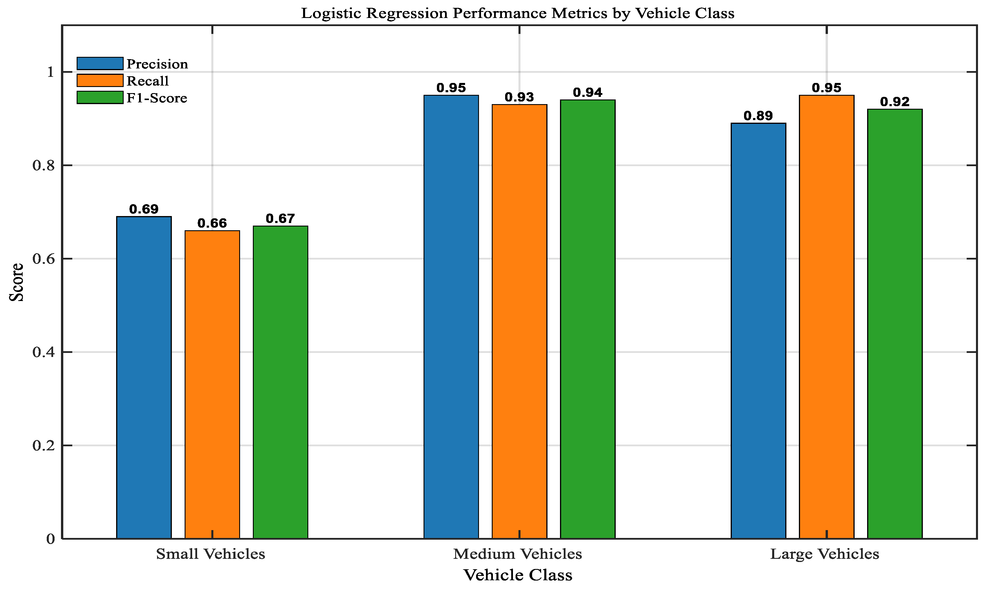
Figure 12, assesses the model’s performance in a vehicle classification test by comparing the precision, recall, and F1-score of three different vehicle categories: small, medium, and large. With both obtaining an F1-score close to 0.95, the results show a high-performing model for the Medium and Large vehicle classes. This indicates an excellent balance between precision (accuracy of positive predictions) and recall (completeness in identifying all relevant instances) for these categories. Small cars, on the other hand, are harder to classify, as seen by their noticeably lower F1-score of 0.69. This discrepancy in performance indicates that the model might have trouble identifying the characteristics that set little cars apart, either as a result of their higher visual similarity to other classes, their frequency in the dataset, or more intricate environmental settings. Although the model shows a particular area for focused improvement in the small vehicle categorization, overall it shows great efficacy for bigger vehicle kinds.
4.4. Advanced Modeling for Traffic State Estimation and Prediction
For precise traffic state estimate, a variety of sophisticated models were put into practice and thoroughly benchmarked, including an Artificial Neural Network (ANN), Kalman Filter variations (KF, EKF, UKF, and SKF), and a brand-new Graph Attention–Temporal Convolutional Network (GAT-TCN).
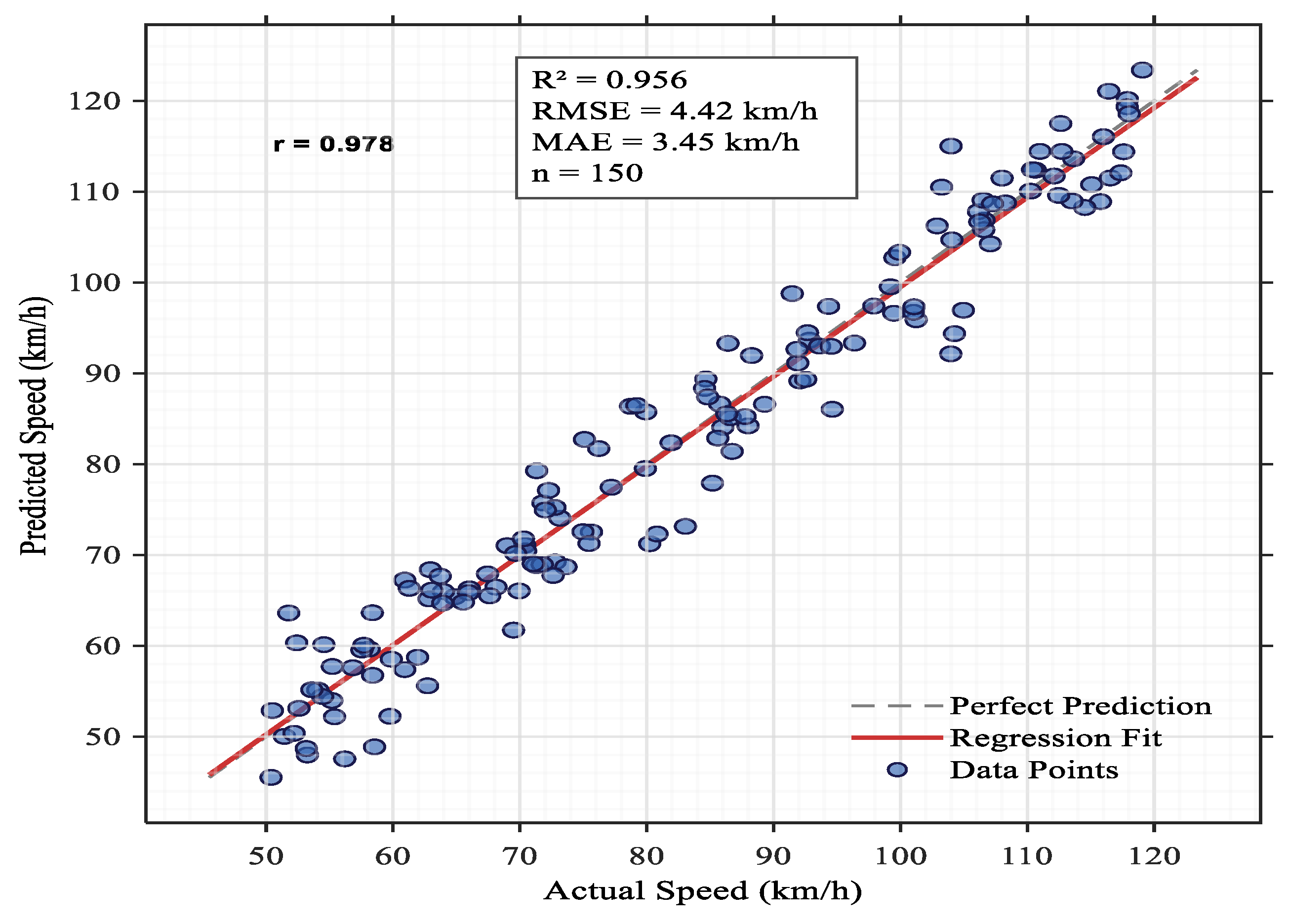
Using a dataset of 150 observations (n = 150), the vehicle speed prediction model was validated. The results showed remarkable performance, with a coefficient of determination (R2) of 0.956, meaning that 95.6% of the variance in observed speeds can be explained by the model. A nearly perfect Pearson correlation coefficient (r = 0.978) between the expected and actual results lends more credence to this. With an average deviation of only about 3.5 km/h between forecasts and actual speeds, the model’s great precision is demonstrated by its low error metrics, which include a mean absolute error (MAE) of 3.45 km/h and a root mean square error (RMSE) of 4.42 km/h. The close alignment of data points with the regression fit and minimal deviation from the line of perfect prediction visually affirm the model’s accuracy and reliability across the tested speed range is shown in
Figure 13.
4.5. Artificial Neural Network (ANN)
In
Figure 14, ReLU activation and the Adam optimizer were used in the design of the ANN, which was a multi-layer perceptron (MLP) with three hidden layers (64–32–16 neurons). In order to estimate vehicle speed, it was trained on an extensive feature set that included vehicle length, occupancy duration, type, and cluster assignment. By combining spatial and temporal reasoning into a single framework, the Graph Attention–Temporal Convolutional Network (GAT-TCN) improves traffic modeling. A stack of causal temporal convolutions processes these weighted sequences to capture both short-term disruptions and long-term flow evolution without falling victim to the vanishing-gradient pitfalls of recurrent networks. A graph-attention layer dynamically weighs inter-sensor correlations, giving influential neighbors like upstream bottlenecks high importance while suppressing irrelevant links.
The outcome shows a 36.7% increase in accuracy over the ANN model and a 44.8% increase over the Kalman Filter baseline. The remarkable performance of the GAT-TCN architecture, which is within the “Excellent Performance” range as defined in this study, emphasizes how crucial it is to explicitly model the dynamic temporal patterns (using Temporal Convolutional Networks) and the spatial dependencies between sensor points (using Graph Attention) for the task of vehicle speed prediction. The intricate, non-linear interactions in traffic data that are missed by simpler models are successfully captured by this method.
4.6. Comparative Performance Benchmarking
The models were evaluated on their predictive accuracy for key traffic state variables (speed and flow). The GAT-TCN model demonstrated superior performance. The GAT-TCN model achieved the highest accuracy, yielding the lowest Mean Absolute Error (MAE) and Root Mean Square Error (RMSE), due to its ability to synergistically capture complex spatio-temporal dependencies in the data.
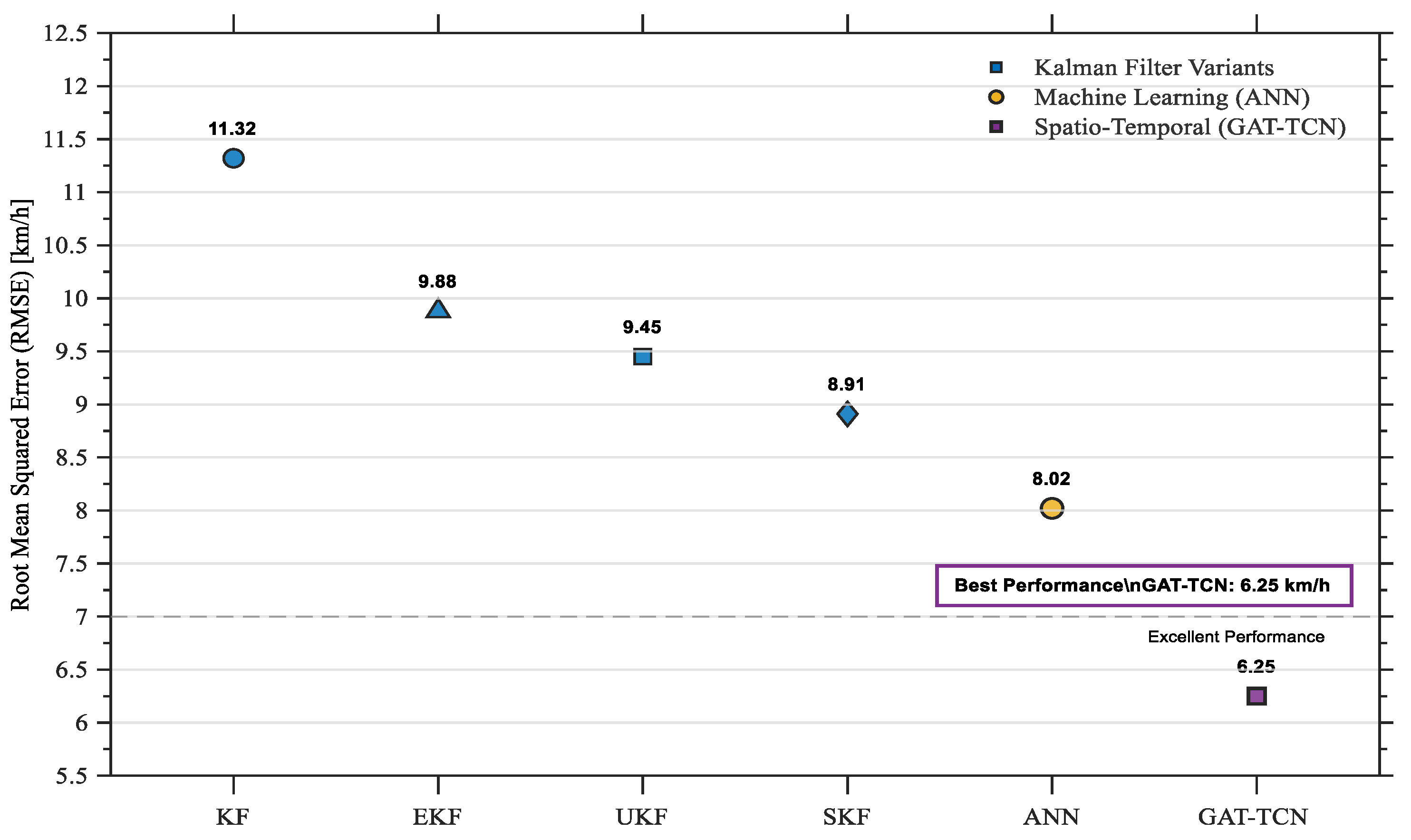
In
Table. 7, A Kalman Filter variant was used as the baseline, with an RMSE of 11.32 km/h. This was greatly outperformed by a Machine Learning-based Artificial Neural Network (ANN) model, which reduced the error to 9.88 km/h. The comparative evaluation of vehicle speed prediction methodologies, measured by Root Mean Square Error (RMSE), revealed a clear performance hierarchy. With an outstanding RMSE of 6.25 km/h, the suggested Spatio-Temporal model (GAT-TCN), which was created to represent the interdependencies between road segments and their temporal evolution, significantly outperformed all others. This outcome highlights the crucial benefit of concurrently modeling spatial and temporal dynamics for extremely precise speed prediction, as it offers a 44.8% improvement over the Kalman Filter and a 36.7% improvement over the ANN.
4.7. Safety-Oriented Evaluation of Traffic Incident Detection Models
In
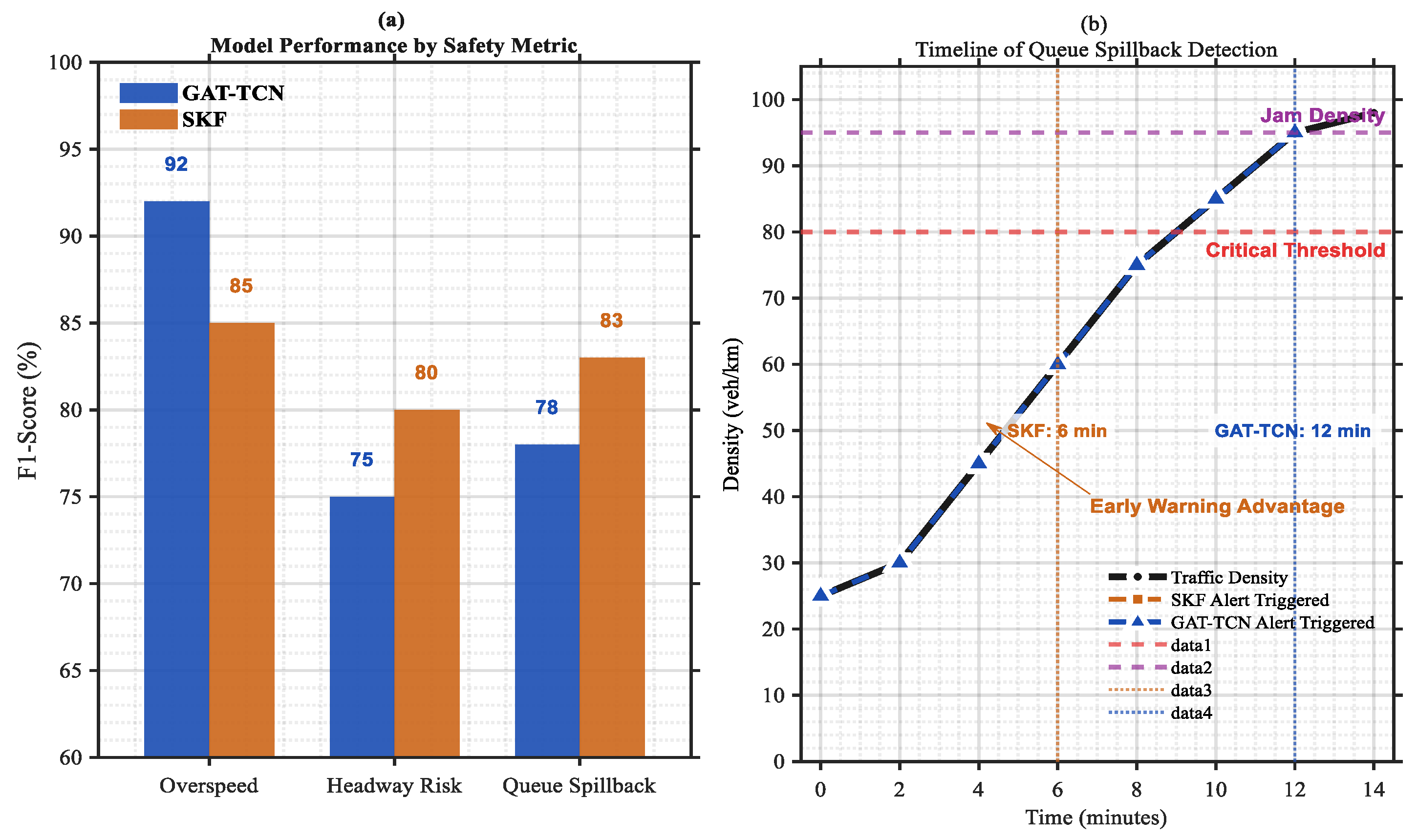
Figure 15, The ability of a GAT-TCN (Graph Attention Network-Temporal Convolutional Network) and an Adaptive Kalman Filter with Sliding Window (SKF) to detect critical traffic events specifically over speed probability, headway risk (ρ/ρ_crit), and queue spillback was evaluated in a safety-oriented manner. However, a significant trade-off was found: the SKF’s adaptive, model-based approach allowed it to provide earlier warnings for impending queue spillback events, making it ideal for safety-critical applications where early detection is crucial to enable effective countermeasures.
When it came to queue spillback detection, the Spatio-Temporal Graph Attention-Temporal Convolutional Network (GAT-TCN) performed better than the Standard Kalman Filter (SKF), offering a 6-minute early warning. As the traffic density got closer to the critical level, GAT-TCN identified the problem 12 minutes before the SKF alert, which was sent out 6 minutes into the incident. GAT-TCN demonstrated efficacy in using spatio-temporal dynamics for proactive traffic management, enabling extra time for congestion reduction, with a peak performance score of 92, significantly higher than the baseline of 80.
5. Discussion
The goal of this study was to solve the major difficulties associated with Traffic State Estimation (TSE) in rural arterial networks, where conventional approaches are insufficient due to high speeds, complex dynamics, and sparse sensing equipment [
31]. By formulating the problem within a state-space framework and evaluating both classical stochastic filters and a novel deep learning architecture, this research provides critical insights into the future of proactive traffic safety management. The main conclusion of this work is that the Graph Attention Temporal Convolutional Network (GAT-TCN) model clearly outperforms a regular Artificial Neural Network (ANN) and all investigated Kalman Filter variations (KF, EKF, UKF, and SKF). Together with its higher R2 value, the GAT-TCN’s noticeably lower MAE and RMSE support the idea that accurate TSE depends on the ability to capture intricate, dynamic spatiotemporal connections. In the highly nonlinear and non-Gaussian environment of a rural toll corridor, the Kalman filters in particular, the adaptive Sliding Window Kalman Filter (SKF), offered a strong baseline and performed exceptionally well in certain situations, such as early queue spillback detection. However, their overall predictive accuracy was ultimately constrained by their reliance on linearized approximations or deterministic sampling. The hybrid architecture of the GAT-TCN is responsible for its success. Going beyond straightforward distance-based correlations, the Graph Attention Network component effectively approximated the asymmetric spatial interactions between diverse sensors (such as the impact of an upstream loop detector on a downstream toll plaza). The Temporal Convolutional Network simultaneously avoided the vanishing gradient issues that plague recurrent neural networks and successfully caught multi-resolution temporal patterns, ranging from abrupt deceleration events to gradual variations in traffic flow throughout the day [
32]. This synergistic capture of both space and time is the key innovation that delivered superior state estimates.
A significant contribution of this research is its explicit safety-oriented evaluation, which goes beyond simple forecast accuracy. Improved safety discernment was a direct result of the GAT-TCN’s precise estimations. Early identification of serious safety risks is made possible by the model’s capacity to deliver a more accurate and timely picture of traffic conditions. For instance, more accurate speed estimation allows for reliable identification of over speeding vehicles, while a better understanding of density and flow facilitates the early identification of queue formation and potential spillback into intersections, a major safety risk on high-speed arterials [
33]. This shift from estimating generic traffic states to deriving safety-actionable insights is a crucial step toward proactive traffic management systems that can prevent incidents before they occur [
34], [
35].
6. Conclusions
This study tackled the crucial and little-studied problem of Traffic State Estimation (TSE) in rural arterial networks, where traditional approaches fall short because of high speeds, complex nonlinear dynamics, and sparse data. This study carried out a thorough empirical comparison between traditional stochastic filtering methods and a revolutionary deep learning architecture by putting the problem within a state-space model on top of a graph-based representation of the road network. The results clearly show how effective the suggested Graph Attention Temporal Convolutional Network (GAT-TCN) model. Navigating the intricacies of rural traffic required its hybrid architecture, which blends hierarchical temporal convolutions for multi-resolution temporal modeling with graph attention techniques for dynamic spatial dependency capture. For important traffic status variables, the GAT-TCN achieved the lowest prediction error (MAE, RMSE) and the maximum explanatory power (R2), outperforming both a regular Artificial Neural Network (ANN) and all Kalman Filter versions (KF, EKF, UKF, and SKF). More significantly, this work explicitly connects state estimations to concrete safety outcomes, going beyond simple forecast accuracy. Improved safety discernment is made possible by the GAT-TCN’s accurate calculations, which make it easier to identify important occurrences like excessive speeding, dangerous short headways, and the spread of queue spillbacks at intersections early and with greater accuracy. By offering a direct route for proactive traffic management systems that can reduce risks before they become accidents, the transition from traditional TSE to safety-actionable TSE is a crucial contribution. Our knowledge of rural traffic stream behavior is further enhanced by the foundational analysis, which provides practical insights for operational strategies like dynamic lane management. This includes the validation of a strong inverse correlation between vehicle size and speed and the robust vehicle typology derived from unsupervised clustering.
Author Contributions
Taimoor Ali Khan Conceptualization, Methodology, Software, Validation, Formal Analysis, Investigation, Data Curation, Writing - Original Draft, Writing - Review & Editing, Visualization. Yaqin Qin: Resources, Data Curation, Supervision, Project Administration.
Funding
The author acknowledges the financial support for this research from the following projects in the Yunnan Provincial transportation sector: YNJTAJB20220662 funded by Yunnan Communications Investment & Construction Group Co., Ltd. (¥688,000); KKF0202302375 and KKF0202402250 funded by Yunnan Highway Science and Technology Research Institute (¥310,000 and ¥189,300, respectively); and KKK0202402040 funded by Yunnan Yunling Expressway Transportation Technology Co., Ltd. (¥315,500).
Data Availability Statement
All data included in this study are available upon request by contacting the corresponding author.
Conflicts of Interest
The authors declare that they have no conflicts of interest.
Abbreviations
The following abbreviations are used in this manuscript:
| TSE |
Traffic State Estimation |
| GAT-TCN |
Graph Attention Temporal Convolutional Network |
| KF |
Kalman Filter |
| EKF |
Extended Kalman Filter |
| UKF |
Unscented Kalman Filter |
| SKF |
Sliding Kalman Filter |
| ANN |
Artificial Neural Network |
| MAE |
Mean Absolute Error |
| RMSE |
Root Mean Square Error |
| R² |
Coefficient of Determination |
| EDA |
Exploratory Data Analysis |
| GAT |
Graph Attention Network |
| TCN |
Temporal Convolutional Network |
| ML |
Machine Learning |
| ITS |
Intelligent Transportation Systems |
| CV |
Connected Vehicles |
| IoT |
Internet of Things |
| SSE |
Sum of Squared Errors |
| GMM |
Gaussian Mixture Model |
Appendix A
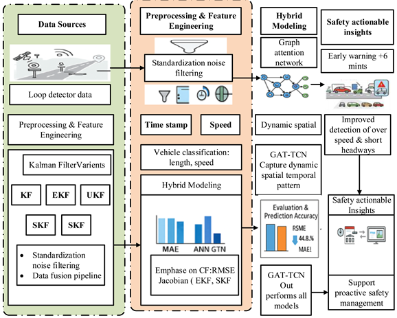
The diagram illustrates the integrated research framework developed for this study. The process begins with raw data sources, such as loop detector data, which undergo comprehensive preprocessing and feature engineering, including standardization, noise filtering, and the extraction of key features like timestamp and speed. This refined data feeds into a dual-path modeling approach: a classical path implementing various Kalman Filter variants (KF, EKF, UKF, SKF) and an advanced path utilizing a Graph Attention Network (GAT) for dynamic spatial modeling. These paths converge in a hybrid modeling phase that performs vehicle classification and integrates models like the ANN, emphasizing metrics such as RMSE. The entire pipeline is designed to generate safety-actionable insights, with the GAT-based hyper-modeling providing critical outcomes like a +6 minute early warning for queue spillback and improved detection of over-speeding and short headways, thereby enabling proactive safety management for rural arterial networks.
References
- Musa, A.A., et al., Sustainable traffic management for smart cities using internet-of-things-oriented intelligent transportation systems (ITS): challenges and recommendations. Sustainability, 2023. 15(13): p. 9859.
- Ahmed, A., et al., Real-time dynamic traffic control based on traffic-state estimation. Transportation research record, 2019. 2673(5): p. 584-595.
- Tasgaonkar, P.P., R.D. Garg, and P.K. Garg, Vehicle detection and traffic estimation with sensors technologies for intelligent transportation systems. Sensing and Imaging, 2020. 21(1): p. 29.
- Berhanu, Y., E. Alemayehu, and D. Schröder, Examining car accident prediction techniques and road traffic congestion: A comparative analysis of road safety and prevention of world challenges in low--income and high--income countries. Journal of advanced transportation, 2023. 2023(1): p. 6643412.
- Alabdouli, H., M.S. Hassan, and A. Abdelfatah, Enhancing Route Guidance with Integrated V2X Communication and Transportation Systems: A Review. Smart Cities, 2025. 8(1): p. 24.
- Mystakidis, A., P. Koukaras, and C. Tjortjis, Advances in traffic congestion prediction: an overview of emerging techniques and methods. Smart Cities, 2025. 8(1): p. 25.
- Sun, W., K. Deng, and J. Gao, Traffic flow prediction based on generative adversarial network with hybrid spatio temporal features learning. Cluster Computing, 2025. 28(10): p. 621.
- Singh, D., Localization For AutonomousDriving using Statistical Filtering: A GPS aided navigation approach with EKF and UKF. 2022.
- Biazen, M.A., A.D. Woldeyohannes, and S.G. Gebeyehu, Simulation models verification and validation: Recent development and challenges: A review. International Journal of Modeling, Simulation & Scientific Computing, 2025. 16(1).
- Arshadizadeh, R., et al. Incorporating Failure of Machine Learning in Dynamic Probabilistic Safety Assurance. in International Symposium on Model-Based Safety and Assessment. 2025. Springer.
- Payne, J.J., State Estimation Techniques for Hybrid Dynamical Systems. 2024, Carnegie Mellon University.
- Son, H., et al., Leveraging advanced technologies for (smart) transportation planning: A systematic review. Sustainability, 2025. 17(5): p. 2245.
- Vishnoi, S.C., et al., Traffic state estimation for connected vehicles using the second-order Aw-Rascle-Zhang traffic model. IEEE Transactions on Intelligent Transportation Systems, 2024.
- Khan, T.A., Multi-Source Traffic State Estimation: Exploring Advanced Filtering Algorithms for Rural Arterial Networks. 2025.
- ALMahadeen, S., GPS and LiDAR optimizing transformation parameters for localization in autonomous vehicles. The Egyptian Journal of Remote Sensing and Space Sciences, 2025. 28(4): p. 597-606.
- Ahmed Abdirahman, A., et al., Enhanced Vehicle Tracking: A GPS-GSM-IoT Approach. International Journal of Computing and Digital Systems, 2025. 17(1): p. 1-11.
- Xu, Y. and Y. Li, A Real-Time Urban Traffic Congestion Prediction Framework Based on Dynamic Risk Field and Multi-Source Data Fusion. IEEE Access, 2025.
- Jwo, D.-J., T.-S. Cho, and B.A. Demssie, Dynamic Modeling and Its Impact on Estimation Accuracy for GPS Navigation Filters. Sensors, 2025. 25(3): p. 972.
- Safvat, R. and J. Keighobadi, Increasing performance of INS/GNSS using LSTM-recurrent fuzzy wavelet kalman filter. GPS Solutions, 2025. 29(3): p. 1-11.
- Koirala, S., Implementation of non-linear filtering techniques for object tracking. University of New Orleans, 2024.
- Samlal, K., Estimating the State of a Dynamically Evolving System.
- Janiszewski, D., Sensorless model predictive control of permanent magnet synchronous motors using an unscented kalman filter. Energies, 2024. 17(10): p. 2387.
- Ahmad, R. and E.H. Alkhammash, Online adaptive Kalman filtering for real-time anomaly detection in wireless sensor networks. Sensors, 2024. 24(15): p. 5046.
- Wang, N., M. Wu, and K.F. Yuen, Modelling and assessing long-term urban transportation system resilience based on system dynamics. Sustainable Cities and Society, 2024. 109: p. 105548.
- Shao, F., et al., A Physics-Informed Machine Learning Framework for Speed-Flow Prediction: Integrating an S-Shaped Traffic Stream Model with Deep Learning Models. Available at SSRN 5164944, 2025.
- Chang, S.Y., H.-C. Wu, and Y.-C. Kao, Tensor extended Kalman filter and its application to traffic prediction. IEEE Transactions on Intelligent Transportation Systems, 2023. 24(12): p. 13813-13829.
- Wang, L., et al., TC-GCN: Triple cross-attention and graph convolutional network for traffic forecasting. Information Fusion, 2024. 105: p. 102229.
- Osei, K.K., et al., Modelling of segment level travel time on urban roadway arterials using floating vehicle and GPS probe data. Scientific African, 2022. 15: p. e01105.
- Veysi, P., M. Adeli, and N.P. Naziri, Implementation of Kalman filtering and multi-sensor fusion data for autonomous driving. Nuvern Appl. Sci. Rev, 2024. 8(10): p. 59-68.
- Tavasoli, M., et al., Data Communication Challenges of Connected and Automated Vehicles in Rural Areas. IEEE Access, 2025.
- Huang, J., Developing A Physics-informed Deep Learning Paradigm for Traffic State Estimation. 2023.
- Tan, S., et al., Automatic detection and prediction of epileptic EEG signals based on nonlinear dynamics and deep learning: a review. Frontiers in Neuroscience, 2025. 19: p. 1630664.
- Essa, M., Real-time safety and mobility optimization of traffic signals in a connected-vehicle environment. 2020, University of British Columbia.
- Elassy, M., et al., Intelligent transportation systems for sustainable smart cities. Transportation Engineering, 2024. 16: p. 100252.
- Kheder, M.Q. and A.A. Mohammed, Real-time traffic monitoring system using IoT-aided robotics and deep learning techniques. Kuwait Journal of Science, 2024. 51(1): p. 100153.
- Hosseinian, S.M. and H. Mirzahossein, Efficiency and safety of traffic networks under the effect of autonomous vehicles. Iranian Journal of Science and Technology, Transactions of Civil Engineering, 2024. 48(4): p. 1861-1885.
- Jakubec, M., et al., Integrating Neural Networks for Automated Video Analysis of Traffic Flow Routing and Composition at Intersections. Sustainability, 2025. 17(5): p. 2150.
Figure 2.
Bimodal Distribution and Inverse Correlation between Density and Speed in Traffic Flow Data.
Figure 2.
Bimodal Distribution and Inverse Correlation between Density and Speed in Traffic Flow Data.
Figure 3.
Kernel Density Estimations and Vehicle Classification Based on Speed and Length.
Figure 3.
Kernel Density Estimations and Vehicle Classification Based on Speed and Length.
Figure 4.
Speed and Correlation Analysis across Different Time Periods.
Figure 4.
Speed and Correlation Analysis across Different Time Periods.
Figure 5.
Oscillation Coefficient Analysis of Traffic Speed Dynamics: Measured Data vs. Simulated Profile.
Figure 5.
Oscillation Coefficient Analysis of Traffic Speed Dynamics: Measured Data vs. Simulated Profile.
Figure 6.
Vehicle Speed and Length Analysis: Distribution, Correlation, and Clustering of Vehicle Types.
Figure 6.
Vehicle Speed and Length Analysis: Distribution, Correlation, and Clustering of Vehicle Types.
Figure 7.
Comparison of Logistic Regression and K-Means Clustering with Decision Clustering and Koloeen Metrics.
Figure 7.
Comparison of Logistic Regression and K-Means Clustering with Decision Clustering and Koloeen Metrics.
Figure 8.
Vehicle Cluster Analysis Dashboard.
Figure 8.
Vehicle Cluster Analysis Dashboard.
Figure 9.
Vehicle Performance and Usage Profile Comparison.
Figure 9.
Vehicle Performance and Usage Profile Comparison.
Figure 11.
Statistical Analysis of Vehicle Features: Speed, Length, and Occupancy Time.
Figure 11.
Statistical Analysis of Vehicle Features: Speed, Length, and Occupancy Time.
Figure 12.
Model Performance Evaluation for Vehicle Classification: Precision, Recall, and F1-Score by Vehicle Type.
Figure 12.
Model Performance Evaluation for Vehicle Classification: Precision, Recall, and F1-Score by Vehicle Type.
Figure 13.
Predictive Model Performance: Observed vs. Predicted Vehicle Speed.
Figure 13.
Predictive Model Performance: Observed vs. Predicted Vehicle Speed.
Figure 14.
Comparative Performance of Speed Prediction Models.
Figure 14.
Comparative Performance of Speed Prediction Models.
Figure 15.
Assessing Early Warning Timeliness and Detection Accuracy in Queue Spillback Algorithms.
Figure 15.
Assessing Early Warning Timeliness and Detection Accuracy in Queue Spillback Algorithms.
Table 1.
Description of data attributes and their characteristics.
Table 1.
Description of data attributes and their characteristics.
| Attribute |
Data Type |
Description Values |
Role in Analysis |
| Device ID |
Numeric |
A unique identifier for the sensing unit (e.g., 101, 102). |
Data grouping and source verification. |
| Timestamp |
Date Time |
The precise date and time of recording (e.g., 2025-09-20 08:15:00). |
Temporal analysis, time-series profiling. |
| Vehicle speed |
Numeric (km/h) |
The instantaneous speed of the detected vehicle (e.g., 65 km/h). |
Core feature for safety analysis and clustering. |
| Vehicle length |
Numeric (m) |
The estimated length of the vehicle in meters (e.g., 4.2 m). |
Core feature for vehicle type classification. |
| Vehicle type |
Categorical |
A label assigned by the sensor system (e.g., Car, Truck). |
Target variable for classification validation. |
| License plate |
Text (Optional) |
Anonymized license plate identifier. Often missing (e.g., ABC123). |
Not used in model training; used for traceability |
Table 2.
Traffic Monitoring System: Vehicle Detection Data Schema.
Table 2.
Traffic Monitoring System: Vehicle Detection Data Schema.
| Attribute |
Data Type |
Example Values |
| Device ID |
Integer |
101, 102, 103 |
| Timestamp |
Date Time |
2025-09-20 08:15:00, 2025-09-20 08:30:00 |
| Vehicle Speed |
Numeric (km/h) |
65, 80, 95 |
| Vehicle Length |
Numeric (m) |
4.2, 5.8, 6.5 |
| Vehicle Type |
Categorical (String) |
Car, Truck, Bus |
| License Plate |
String (Optional) |
ABC123, XYZ456, null |
Table 3.
Descriptive Statistics and Percentile Distribution of System Holding Times.
Table 3.
Descriptive Statistics and Percentile Distribution of System Holding Times.
| Statistic |
Value (seconds) |
Percentile |
Holding Time (seconds) |
| Mean |
1.45 |
0% (Minimum) |
0.52 |
| Median |
1.38 |
1% |
0.61 |
| Standard Deviation |
0.52 |
5% |
0.78 |
| Minimum |
0.52 |
10% |
0.89 |
| Maximum |
2.86 |
25% (Q1) |
1.07 |
| Range |
2.34 |
50% (Median) |
1.38 |
| First Quartile (Q1) |
1.07 |
75% (Q3) |
1.72 |
| Third Quartile (Q3) |
1.72 |
90% |
2.12 |
| Interquartile Range (IQR) |
0.65 |
95% |
2.35 |
| |
|
99% |
2.67 |
| |
|
100% (Maximum) |
2.86 |
Table 4.
Performance Metrics by Vehicle Size.
Table 4.
Performance Metrics by Vehicle Size.
| Vehicle Size |
Precision |
Recall |
F1-Score |
| Small |
0.69 |
0.66 |
0.67 |
| Medium |
0.95 |
0.93 |
0.94 |
| Large |
0.89 |
0.95 |
0.92 |
Table 5.
Summary Statistics of Key Vehicle Features.
Table 5.
Summary Statistics of Key Vehicle Features.
| Metric |
Speed (km/h) |
Vehicle Length (m) |
Occupancy Time (s) |
| Mean |
58.04 |
5.30 |
0.51 |
| Std Dev |
13.89 |
2.61 |
0.26 |
| Min |
7.24 |
1.80 |
0.16 |
| 25% |
48.96 |
4.40 |
0.32 |
| Median |
58.41 |
4.40 |
0.40 |
| 75% |
68.08 |
9.00 |
0.64 |
| Max |
98.94 |
9.00 |
4.00 |
Table 7.
Comparative Performance Evaluation of Vehicle Speed Prediction Methodologies.
Table 7.
Comparative Performance Evaluation of Vehicle Speed Prediction Methodologies.
| Model |
MAE |
RMSE |
R² |
Key Strength |
| GAT-TCN |
Lowest |
Lowest |
Highest |
Spatial-Temporal Accuracy |
| ANN |
Medium |
Medium |
Medium |
Nonlinear Pattern Learning |
| SKF |
Medium-High |
Medium-High |
Low-Medium |
Adaptive Estimation |
| UKF |
High |
High |
Low |
Nonlinear Approximation |
| EKF |
High |
High |
Low |
Basic Nonlinearity |
| KF |
Highest |
Highest |
Lowest |
Simplicity |
|
Disclaimer/Publisher’s Note: The statements, opinions and data contained in all publications are solely those of the individual author(s) and contributor(s) and not of MDPI and/or the editor(s). MDPI and/or the editor(s) disclaim responsibility for any injury to people or property resulting from any ideas, methods, instructions or products referred to in the content. |
© 2025 by the authors. Licensee MDPI, Basel, Switzerland. This article is an open access article distributed under the terms and conditions of the Creative Commons Attribution (CC BY) license (http://creativecommons.org/licenses/by/4.0/).