Precision Agriculture-Based Pest Detection Solutions Using AI Algorithms Simulated with Complex Logic Gates Integration and 3D Bioprinting

1. Introduction

Algorithms are essential to improving the capabilities and efficiency of artificial intelligence (AI) and its integration with other technologies in the quickly developing field of computer science and its substitutes. The main areas of focus include cloud computing, blockchain technology, robotics and automation and mobile applications apart from machine learning and deep learning. The present set of studies explores and covers a number of important elements of AI algorithms, offering a thorough systematic framework for comprehending their relative efficacy, Internet of Things (IoT) integration, mobile application optimization, and the creation of intuitive user interfaces. The creation and the further development of lightweight AI models is essential in the field of mobile applications especially those that are centred on real-time detection like agricultural crop pest diagnosis. For these models to function at their best on devices with limited resources, they must effectively analyse data and simultaneously lower the computational expenses. Examining various pest detection algorithms, evaluating their computing costs, accuracy scores and efficiency ratings are emphasized. It also emphasizes how crucial algorithm optimization is to improving the performance of mobile applications.

The cost and efficiency of calculations are greatly impacted by the type of the algorithms used. Mobile apps that must function with limitations with conditions like battery life and processing power, the use of efficient algorithms can result in quicker reaction times leading to lower memory utilisation. Quicksort and binary search can be taken as examples where algorithms with lower temporal complexity are preferred for sorting and searching tasks because they can handle larger datasets more efficiently. Algorithm efficiency is commonly assessed in terms of time complexity and it is the sum of operations required as a function of input size and space complexity which is the amount of memory used during calculation. These measurements are crucial for comprehending how an algorithm functions in different situations especially in scenarios where the amount of the inputs increases. The entire set of resources needed for data processing and transfer is also included in computational costs. First resource is the one which computes the amount of time that is needed to finish a task or group of assignments called as the execution time. Second is the energy consumption as it is important for mobile devices where the battery life is problematic. The third resource involves the usage of memory, it calculates the amount of RAM used during execution. A careful balance between speed, memory usage, and energy consumption is necessary to optimize these expenses. This can be applied on the usage of parallel computing techniques that can drastically shorten execution time by dividing work across several processors.

Analysing the computational costs and efficiency of different algorithms that are used in detecting pests Support Vector machines have a higher computational cost with O(n^2) time complexity than the decision trees having O(n log n) and moderate computational costs. While K-nearest neighbours shows intermediate efficiency with O(n^2) time complexity, neural networks display fluctuating efficiency scores with extremely high computational costs (O(n^3)). The following analysis shows that although certain algorithms may have high efficiency ratings, they can also be computationally expensive making them less suitable choice for mobile applications where resource limitations are important.

At last, the potential synergistic combination of 3D bioprinting and logic gates in transforming agricultural pest detection is explored. 3D bioprinting is an advanced and upcoming technique that enables the layer-by-layer construction of three-dimensional objects and it has immense potential in various fields including agriculture. It prints biological materials like cells and tissues and offers a possibility of creating living structures with specific functions. Logic gates is the fundamental building blocks of digital circuits that can be integrated into biosensors and other devices to detect and analyse incoming biological signals. These devices can be used to monitor crop health, identify pests, and trigger specific responses, such as the release of biocontrol agents. This paper also highlights the exciting possibilities of combining these two technologies to create novel solutions for agricultural pest detection.

2. Comparative Analysis and Evaluation of AI Algorithms in Agricultural Pest Detection

A range of performance indicators and parameters are used to evaluate AI algorithms offering insights into their efficacy in various tasks. Important metrics for classification are recall that can be used for the model's capacity to find all pertinent instances. Thereafter, accuracy quantifies the percentage of correct predictions. Precision indicates the accuracy of positive predictions and its equivalent F1 score can strikes a balance concerning both the precision and recall particularly in cases where datasets are unbalanced. A confusion matrix provides a comprehensive breakdown of true and false classifications which classifies the accuracy or support of a model. The AUC-ROC metric checks a model's ability to do a comparison between classes. Mean Squared Error (MSE) emphasizes larger errors by squaring differences. Relevant indicators for regression tasks include Mean Absolute Error (MAE) measuring the average absolute variance among predicted and actual values, and Root Mean Squared Error (RMSE) presenting the error in the same units as the target variable. The degree to which the independent factors account for the range in the dependent variable is represented by the R-squared (R²). Choosing the right measurements is essential in understanding model performance and arriving at well-informed selections regarding enhancements.

2.1. Random Forest

Throughout training, Random Forest generates a large number of decision trees and produces the mean prediction (regression) and the class mode (classification) for each individual decision tree. The basis of this classification in plant disease detection is the extraction of important features from leaf images, which are necessary for differentiating between healthy and sick plant portions. Using an ensemble technique along with RF improves prediction accuracy and manages overfitting, the two important aspects of managing large datasets such as plant disease detection databases (Xian et al., 2021). High accuracy rates have been achieved by researchers using RF to efficiently treat a variety of plant diseases. For example, research has demonstrated that RF can identify diseases like bacterial spot and blight found on leaves with up to 98% accuracy when image processing methods are used to leaf images (Xian et al., 2021). In a comparative research study, RF was found to perform more accurately and efficiently for datasets involving tomato plant leaves than other classifiers like Support Vector Machines and Decision Trees (Xian et al., 2021). RGB and HSV are the key colour features that assess the distribution of colours in different colour spaces,

Figure 1. Demonstration of flow chart of Random Forest algorithm.

Figure 1. Demonstration of flow chart of Random Forest algorithm.

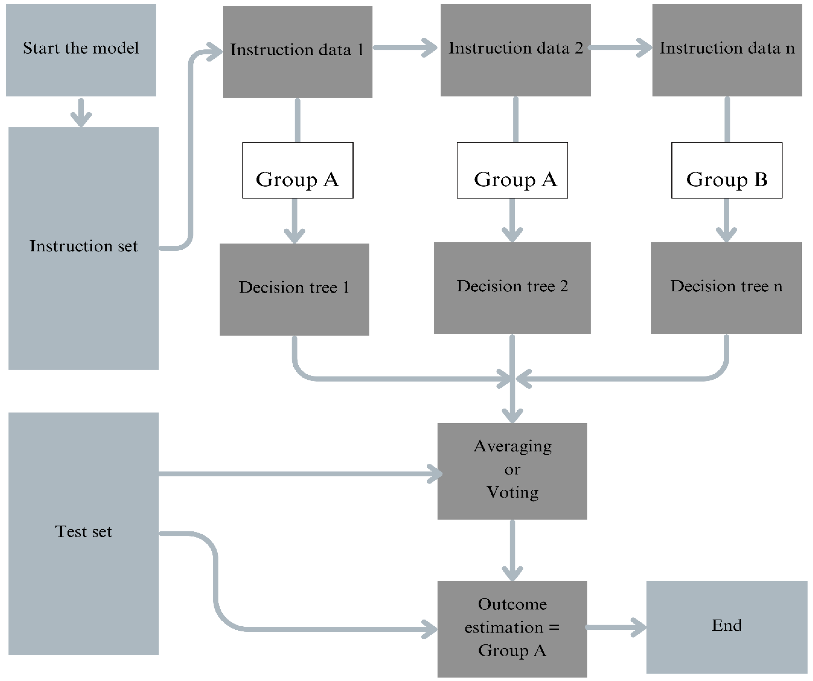
Vein patterns, aspect ratio, perimeter, and area are few examples of form characteristics that aid in the identification of morphological alterations linked to diseases (Xian et al., 2021). The algorithm SIFT and Canny edge detection are the edge detection methods that can highlight impacted areas by identifying the distinct patterns and edges. Finally, depending on geometric qualities, statistical data such as Hu moments describe the shape of the leaf. These many feature sets can be combined to improve disease detection systems in agriculture and increase classification accuracy by RF classifiers' ability to compare and evaluate leaf images (Demilie and Wubetu, 2024). These preparatory procedures aid in the separation of diseased leaf segments and the extraction of pertinent characteristics for categorization. Examples of these features are colour histograms and mean colour values. Histogram of Oriented Gradients (HOG) technique and Haralick textures are two important texture features that quantify pixel intensity patterns and capture the leaf surface structure. Common procedures include converting photos to grayscale and then transforming the colour space with HSV, and further extracting features using techniques like Haralick textures and Grey Level Co-occurrence Matrix (GLCM).

2.2. CNN

Since classification algorithm like CNNs are specifically specialized deep learning networks designed to interpret pixel input, they are most appropriate and frequently deployed for image recognition applications. These networks classify leaf pictures on the basis of whether they are healthy or unhealthy in plant disease detection (Shreshta et al., 2020). One benefit of employing CNN model is that they can automatically extract features from images which can save time and complexity compared to manual feature engineering. Various types of CNN designs have been used to improve the capacity for detection. To name a few, architectural models like InceptionV3, MobileNetV2, and EfficientNetB0 use methods like depth wise separable convolutions to lower processing costs while simultaneously improving accuracy and efficacy (Hassan et al., 2021). One of the studies used a dataset containing around 87,848 photos spanning 58 classes of plant diseases to claim a model's accuracy of 99.53% (Hassan et al., 2021). The calibre and volume of the datasets used for training are frequently cited as factors in judging CNN models' effectiveness. Another study utilizing the PlantVillage dataset with models built on the LeNet architecture achieved an accuracy of 99.32% when classifying soybean diseases from images taken in natural settings, lesion segmentation and disease classification (Boulent et al., 2019). Comparing the accuracy levels of CNNs, which can automatically extract intricate features from images are usually higher than those of these techniques. Conventional methods like SVMs and Decision trees can produce accuracies of approximately 70–85%. Whereas in controlled settings, CNNs often achieve 90% or more. When compared to older approaches, CNNs show higher robustness against alterations in illumination and background conditions. The ResNet architectures that handle the vanishing gradient problem such as ResNet50 and ResNet152 mainly use skip connections to make it easier for gradients to flow over deeper networks. Research has indicated that these models are dependable options for challenging classification problems, with plant disease detection tasks achieving accuracies of approximately 95.61%. Other noteworthy architectures that combine multiple filter sizes in one layer to capture different features at different scales are InceptionV3 and InceptionResNetV2. These models have demonstrated high efficiency and accuracy in plant disease detection, frequently obtaining results that are comparable to more complex models with fewer parameters. Variants such as EfficientNetB0 and EfficientNetB3 have been shown to achieve accuracy rates above 98% in certain experiments, and are recognized for their great performance at lower computing costs. The EfficientNet models systematically build up the network's breadth, depth, and resolution. Depth wise separable convolutions are utilized by MobileNet to drastically reduce the number of parameters without sacrificing the model performance. The MobileNetV2 model has shown successful in real-time applications on mobile devices, obtaining accuracy levels of approximately 97% qualifying it for on-field illness detection. The results of various CNN models are determined in Table 1.

2.3. SIFT

A well-known computer vision approach for locating and characterizing local features in leaf images is the Scale-Invariant Feature Transform or in short known as SIFT. Ever since the model development by David Lowe in 1999, SIFT has found widespread use in a variety of applications which includes robotic mapping, object detection, image stitching, and more. Gaussian blurring is used to create a scale space in the first step of SIFT. It utilizes the Difference of Gaussians (DoG) as an effective approximation in place of the Laplacian of Gaussian (LoG) where the same image has different number of values (Guo et al., 2018). This method finds possible turning places at various scales. After possible key points are found, low contrast points and edge responses that could produce erratic features are eliminated by honing in on their locations. Based on local picture gradients, a dominant orientation is assigned to each key point. By taking this step, it is guaranteed that the key point descriptors won't change with rotation. In the end, each key point’s descriptor is produced by examining the gradients in a predetermined area surrounding its location (Guo et al., 2018).

This description is unaffected by changes in scale or rotation and encapsulates the basic qualities of the main idea. SIFT's capacity to extract several characteristics from images makes it extremely successful in recognizing objects under a variety of situations, including partial occlusion and clutter. Changes in light, orientation, and uniform scaling have no effect on the algorithm. It is appropriate for real-world applications where fluctuations of this kind are frequent because it also demonstrates partial invariance to affine distortions. The SIFT algorithm has found its place in fields inclusive of a particular Object recognition, Image stitching for panoramas, 3D modelling, Gesture recognition, Video tracking and Wildlife identification (Piccinini et al., 2012). It is difficult to obtain real-time performance on conventional hardware due to the computationally demanding nature of the standard SIFT implementation. For example, it can take several seconds to extract features and descriptors for about 2000 key points and it is not good for real-time applications.

Figure 2. Demonstration of flow chart of SIFT algorithm.

Figure 2. Demonstration of flow chart of SIFT algorithm.

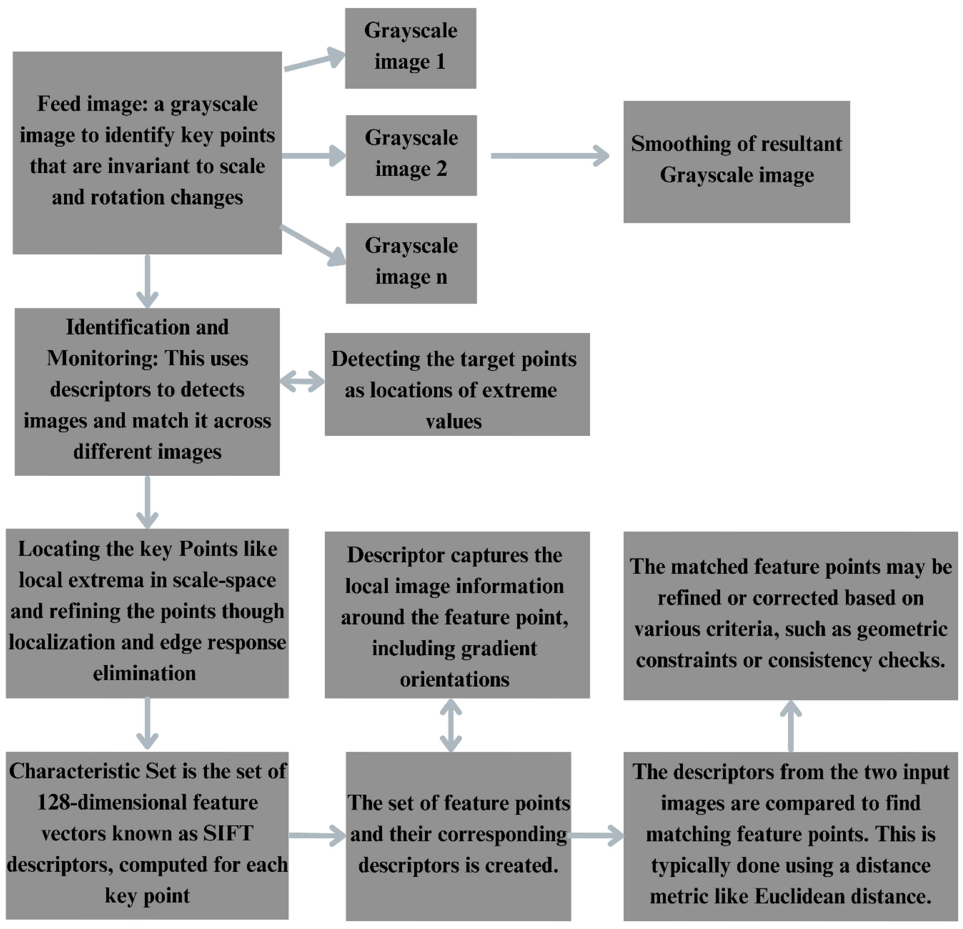
Despite the fact that SIFT might not operate in real time, there are quicker options that might yield results with somewhat lower precision like the Speeded-Up Robust Features (SURF) as well as the binary descriptors like ORB (Oriented FAST and Rotated BRIEF) (Piccinini et al., 2012). The real-time implementation of SIFT is possible with bio-inspired hardware devices that greatly increase processing performance. It is also seen that SIFT makes it possible to identify, differentiate and classify plant diseases with high accuracy, frequently reaching accuracy rates above 90%, when paired with machine learning classifiers such as Support Vector Machines (SVM) and k-Nearest Neighbours (k-NN). Combining SIFT with SVM can diagnose paddy plant illnesses by examining the colours and forms of the leaves with an accuracy of 93.33%.

2.4. HOG

The Histogram of Oriented Gradients (HOG) method is a prominent feature descriptor in computer vision as it is mainly used for problems involving object detection. By examining how gradient orientations are distributed throughout certain regions of an image, it goes on by concentrating on the composition and form of objects. HOG works by determining the gradient orientations and magnitudes in discrete areas of a picture, or also called as "cells." The distribution of edge directions is then represented by a histogram created from these gradients aiding in the identification of structures and forms in the image. The ability of HOG to withstand changes in illumination, viewpoint, and scale is one of its main advantages. This makes it very useful for recognizing pedestrians and other things in a variety of circumstances because of this feature. For sake of maintaining consistency between datasets, the input image is usually downsized to a standard dimension with approximately 128x64 pixels (Rodríguez et al., 2014). Gradients are computed with techniques such as the Sobel operator that highlights intensity variations. The picture is separated into tiny units, such as 8 by 8 pixels. The histogram of each cell is calculated using the gradient orientations (Rodríguez et al., 2014). Cells are normalized by grouping them into larger blocks starting with 2x2 cells. Block histograms are normalized using methods like L2-norm to lessen their sensitivity to variations in light. The normalized histograms from each individual block are concatenated to create the final functional vector. This can be used to feed machine learning classifiers for object detection like Support Vector Machines (SVM) (Dalal et al., 2005). HOG is appropriate for a variety of contexts because it keeps working even in different illumination and orientation conditions. In contrast to deep learning techniques that necessitate large amounts of training data, HOG can function well with smaller datasets. HOG is frequently employed in human detection tasks, outperforming prior approaches such as wavelets and SIFT thanks to its thorough gradient analysis. It is used in real-time as applications in a variety of fields, including autonomous driving systems and surveillance, are made possible by its computing efficiency. CNNs can receive HOG characteristics as extra input layers. A study analysed photos of leaves classified as infected, weak, or healthy in order to identify diseases in chili plants using the HOG algorithm. Harsh leaf, spot leaf, and yellowish leaf conditions were among the illnesses found. There were multiple steps in the approach for identifying illnesses in chili plants. Taking pictures of both healthy and sick chili leaves was part of the data collection process. To improve feature extraction, photos were resized and transformed to the proper colour formats during the pre-processing phase. Then the HOG features were extracted from the pre-processed pictures using a uniform patch size of around 100x200 pixels to guarantee consistency. According to the findings, the Euclidean distance threshold applied during analysis affected the disease diagnosis accuracy. A threshold of 0.0025 produced an average accuracy of 61.6%and the thresholds of 0.0016 and 0.00125 produced improvements of 73.2% and 81.0%, respectively (Dalal et al., 2005). These results demonstrate how HOG may be used as a combination along with machine learning methods to identify disease pattern in chili plants.

2.5. RNN

Recurrent Neural Networks (RNNs) are enhanced in their ability to process sequential data by a number of important properties. They provide efficient memory retention by keeping track of past input information in a concealed state that is updated every time a new step is done. Text creation and machine translation are two applications where RNNs can be most used because of their flexibility in processing sequences of different lengths. They also exchange parameters between time steps enhancing the generalization between various input sequence time points and lowering the model complexity. Different RNN variations have been created to handle particular problem statements like the Vanishing gradient problems which addresses the Long Short-Term Memory (LSTM) networks and its various patterns that allow them to retain information for longer period of time (Fang et al., 2021). The more straightforward option offered by Gated Recurrent Units (GRUs) increases computing efficiency by merging both input and forget gates into a one singular update gate. The Encoder-Decoder architecture is mainly used for tasks like machine translation and it consists of two RNNs where one can encode the input sequence into a fixed-length context vector whereas the other can fully decode it into the output sequence. Bidirectional RNNs process the resulted input sequences in both forward and backward directions to improve context understanding. RNN models find its usefulness in natural language processing for tasks like sentiment analysis and language modelling, speech recognition in systems like Siri and Google Assistant, and time series prediction for financial forecasting and stock price analysis (Fang et al., 2021). Plant images with infected spots is automatically recognized and located by RNNs. This skill is essential for efficient disease classification because it enables the system to ignore unimportant backdrops or sections of healthy plants and concentrate on the pertinent areas of the image that show disease signs. More recently, attention mechanisms have been added to RNNs, improving their capacity to identify important characteristics associated with plant diseases. Assisting the model by prioritizing crucial features and its further integration can raise the accuracy of the pest and plant disease identification. Comparing this to standard CNNs and its subclasses, RNNs have demonstrated a stronger capacity to generalize to unseen infected crop species and various sorts of plant disease imagery. Certain models suggest hybrid designs that combine CNNs and RNNs. By using RNNs for sequence processing and leveraging CNNs' strengths in feature extraction from images, this combination improves the overall classification accuracy for plant diseases.

2.6. GANs

The main application of GANs is data augmentation and it is important when labelled data is hard to come by. It works by taking into account the existing datasets and making a new dataset out of it. GANs aid in the balancing of datasets and enhance the training of machine learning models by producing artificial images of sick plants (Vasudevan and Karthick, 2023). Better training datasets resulted in higher accuracy for diagnosing tomato plant diseases when Conditional GANs (C-GANs) were used to generate synthetic images. One noteworthy method is to use a Tranvolution detection network which improves feature extraction and model performance by fusing CNNs with GAN modules. This approach detected a variety of plant illnesses with an amazing accuracy rate of 51.7%. CNNs and GANs were integrated to enable early detection of infections before serious symptoms appeared, leading to significant accuracy rates in real-time evaluations (Wang et al., 2024). GANs have also been employed in research on rice leaf diseases which is mostly via a subset of its own called as GAN-based data augmentation pipeline. The main difficulties caused by the scarcity of real-world data were partially resolved by this process producing artificial images of rice leaf illnesses. A combination of a Residual Neural Network (MDFC-ResNet) and a Deep Convolutional Generative Adversarial Network (DC-GAN) produced high classification accuracy for a number of rice diseases like the bacterial leaf blight and brown spot and these are mainly found on the leaves. When the suggested model was evaluated against available datasets, it showed an accuracy of up to 97.89%. GANs and CNNs are used in a number of mobile applications that enable users’ farmers in particular to recognize plant diseases from smartphone photos. Developing a cutting-edge technology available in the field can allow for prompt interventions that can reduce crop losses. These tools improve agricultural practice decision-making processes by giving real-time input on plant health.

2.7. SVM

SVM is a supervised deep learning algorithm that can find the optimal hyperplane to separate different classes in a dataset. It is particularly effective in high-dimensional spaces and this feature making it suitable for image classification tasks where features can be numerous. Support Vector Machine algorithms are increasingly finding its usage in the process of identification and classification of plant diseases by analysing images of leaves to distinguish between healthy and infected specimens (Kaur et al., 2015). The process typically involves several key stages like Image Acquisition where plant leaves image is captured, Pre-processing, which enhances image quality through smoothing and segmentation, Feature Extraction, where relevant features are identified using methods like the Gray-Level Co-occurrence Matrix (GLCM) for texture analysis and finally, Classification, where the SVM algorithm is precise as it used to categorize the processed images based on the extracted features. SVM-based approach achieved a classification accuracy of 99.83% when detecting diseases in tomato leaves that utilized a dataset of around 800 images and employing various kernel functions for optimal results. This systematic approach not only aids in the accurate disease detection but also supports timely interventions in agricultural practices. Another approach combined SVM with deep learning techniques, achieving up to 97.2% accuracy in detecting various tomato diseases. Some research has explored hybrid models that integrate SVM with other algorithms such as convolutional neural networks. These models often outperform traditional methods by leveraging the strengths of multiple real-time functional algorithms. SVM-based systems can be implemented on mobile devices, allowing farmers to quickly diagnose plant health issues with minimal training. One of the primary advantages is the great ability of fuzzy systems to handle uncertainty and imprecision in real-world data which is particularly relevant in agricultural settings where environmental factors can affect image quality and disease presentation. Fuzzy SVM assigns membership values to various severity levels of diseases allowing for a nuanced classification that reflects the degree of infection rather than a binary healthy/diseased outcome. This is critical for early intervention. Integrating fuzzy systems with Support Vector Machines (SVM) for plant disease detection offers several significant benefits that enhance the overall performance and reliability of disease classification models. One of the primary advantages is the ability of fuzzy systems to handle uncertainty and imprecision in real-world data and this is particularly relevant in agricultural settings where environmental factors can affect image quality and disease presentation. Fuzzy SVM assigns membership values to various severity levels of diseases, allowing for a nuanced classification that reflects the degree of infection rather than a binary healthy/diseased outcome.

2.8. K-Nearest Neighbours

K-Nearest Neighbours (KNN) is a common supervised machine learning method that is typically used for classification tasks and can also be used to solve regression problems. Classifying a given data point according to the majority class of its closest neighbours in the feature space is the core idea of KNN. It uses metrics such as Manhattan, Minkowski, or Euclidean distances to determine the distance between a point of query and every other point in the training dataset (Uddin et al., 2022). Based on these distances, it then calculates the K-nearest neighbours. KNN averages the values of the K neighbours for regression tasks and assigns the class label that is most common among the algorithm for classification tasks. A large k can result in underfitting by smoothing out significant differences, whereas a small K may cause overfitting because of noise sensitivity. Usually, an odd K is basically selected so that it can avoid classification ties. KNN variants include Ensemble KNN and this combines several KNN models to increase accuracy; Fuzzy KNN, which uses fuzzy logic to handle uncertainty; and Adaptive KNN, which modifies k depending on local data density. KNN has a wide range of uses in medical diagnosis (using patient data record to identify any novel diseases), pattern recognition (in image and audio recognition), and recommendation systems (making product recommendations based on user similarity). The sophisticated variations such as Hassanaat KNN perform better on average over a range of datasets having an accuracy of 64.22% to 83.62% (Taunk et al., 2019). Finding the ideal value of K in the method is essential to getting the best possible model performance and accuracy. For this objective, a number of techniques are usually used. To find the point on the graph when performance gains stop, the Elbow Method plots the accuracy or error rate against different K values creating a "elbow" shape. An ideal K is indicated at this point and it is used to balance the bias and variation. The K-fold cross-validation which comes under Cross-validation divides the dataset into subsets and evaluates performance across several splits to provide a robust assessment of how different K values generalize to unseen data. Often improved by combining it with cross-validation, Grid Search methodically evaluates a range of k values to see which one produces the best results. Despite the need for empirical validation, a popular heuristic called the Rule of Thumb proposes to approximate K as the square root of the dataset size. The last tool for identifying the k that minimizes error or maximum accuracy is an error rate and accuracy plot providing a visual depiction of performance across k values. There are multiple phases involved in the detection of plant diseases. The first step in data collection is compiling a dataset of photos of plant leaves that have been classified as either healthy or linked to particular illnesses. The photos are downsized to a consistent size, improved with methods including sharpening, noise reduction, and contrast adjustment then further segmented to separate the leaf from the backdrop during the image preparation step. The pre-processed images are used to extract pertinent features, including colour features like RGB, HSV, texture features like Gray-Level Co-occurrence Matrix, Local Binary Patterns, and shape features like area, perimeter, and compactness. The dataset is then divided into training and testing sets for KNN classification (Taunk et al., 2019.

Figure 3. Demonstration of flow chart of K-Nearest Neighbours algorithm.

Figure 3. Demonstration of flow chart of K-Nearest Neighbours algorithm.

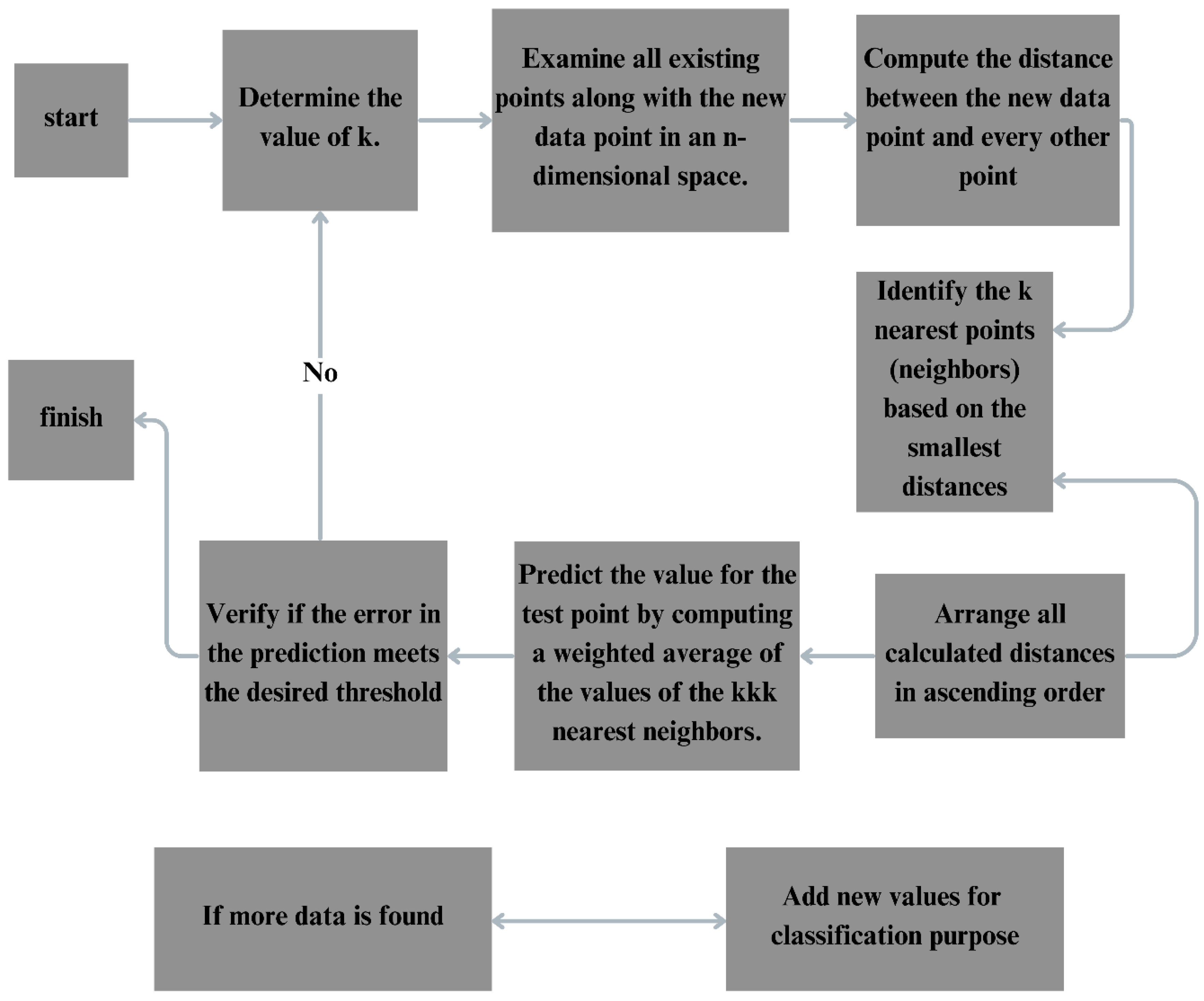
Setting a value for k (the number of neighbours) allows the KNN model to be trained on the training set. Metrics like accuracy, precision, recall, and F1-score are used to assess the performance of the trained model after it has been used to categorize the images in the testing set. The last step in fine-tuning is to optimize the model's performance by varying the value of k and other hyperparameters. One study compared KNN and CNN for detecting diseases in banana leaves and found that CNN achieved a higher accuracy of 90.92% compared to KNN's 67.85%.

2.9. Transformer Networks

Transformers are very useful in a variety of fields because of a few fundamental characteristics that set them apart. Compared to designs like recurrent neural networks (RNNs), their attention mechanism allows the model to better capture context by weighing the significance of various words in a phrase. Transformers greatly speed up training and inference compared to RNNs by using parallel processing to handle every single word in a sentence at once. According to sophisticated theoretical evaluations, transformers can convey higher-order reasoning more effectively than conventional neural networks. By segmenting images into patches and treating them as NLP tokens, Alexey Dosovitskiy et al.'s Vision Transformer (ViT) model in computer vision showed how transformers could manage image classification tasks (Ohagi et al., 2022). On benchmarks, this method has produced state-of-the-art results where it also frequently outperforms methods like CNNs. Transformers are excellent at tasks that call for global contextual awareness and long-range dependencies. ViTs have produced excellent results in image classification on datasets such as ImageNet. They improve object detection by taking into account differences in item size and appearance acting as an essential tool for applications like surveillance and driverless cars (Lee et al., 2019). The attention mechanism also increases the accuracy of semantic segmentation by concentrating on pertinent regions of the image. Transformers are used in image processing, time-series forecasting, reinforcement learning, and biological data analysis, including drug development and DNA sequence interpretation, demonstrating their adaptability beyond their initial application in natural language processing. They are essential for training large language models (LLMs) and are highly effective in question answering, translation, summarization, and sentiment analysis. The revolutionary design ideas of Vision Transformers (ViTs) enable them to effectively manage spatial relationships in images. Initially, they employ a patch-based representation which breaks up images into fixed-size patches (such as 16x16 pixels) and treating each patch as a token, much like NLP words do (Lee et al., 2019). This method preserves the image's overall perspective while enabling the model to examine nearby areas. Positional encodings are introduced to patch embeddings to make up for the absence of intrinsic spatial awareness. This allows the model to capture spatial interactions between patches and provides crucial location information. The fundamental element of ViTs is the self-attention mechanism allowing the model to assess relationships between every patch at once. The methodology makes it easier to capture complex relationships and spatial arrangements by determining the relative relevance of each patch based on attention scores. ViTs accomplish global contextual awareness in a single pass effectively capturing complex spatial relationships and long-range dependencies which in contrast to CNNs depends upon creating only spatial hierarchies over numerous layers (Lee et al., 2019). ViTs improve their capacity to identify objects and relationships in images by identifying abstract patterns and spatial configurations through feed-forward transformations and hierarchical feature learning across many layers of self-attention. This all-encompassing processing method produces better results on a variety of vision tasks.

Vision Transformers (ViTs) successfully handle dynamic and shifting spatial relationships in videos by utilizing temporal modelling approaches and the other architectural improvements. Improvements to temporal modelling, such as the Long and Short-term Temporal Difference. Through variations in successive frames, Vision Transformer (LS-VIT) allows for the recording of both short-term motion details and long-term motion dynamics for reliable spatiotemporal modelling. ViTs can adjust to changing spatial relationships over time thanks to their dual focus. Through the analysis of temporal and spatial correlations within video sequences, the spatio-temporal self-attention mechanism further improves their capabilities. A more detailed understanding of object motion and interactions is made possible by the model's ability to identify pertinent regions while disregarding extraneous noise by calculating attention ratings across frames. By using specific spatial and temporal self-attention mechanisms, techniques like those used in models like Timesformer and ViViT divide films into frame-level components. By reducing computational complexity while maintaining temporal dynamics, this frame segmentation technique makes it possible to handle changing spatial relationships effectively. ViTs can follow object movements and interactions over time thanks to positional encoding modifications, which offer crucial context regarding patch positions within frames and across sequences (Lee et al., 2019). Identification of plant diseases has been transformed by recent developments in vision transformer models. TrIncNet is a lightweight vision transformer made specifically for this use, substituting a unique inception block for the conventional Multi-Layer Perceptron (MLP) in ViTs to enhance feature extraction from diseased images while lowering computing expenses. The vanishing gradient issue is addressed by including skip connections. On the PlantVillage and Maize disease datasets, TrIncNet outperformed other ViT models and conventional CNN architectures by 2.87% and 5.38% in terms of testing accuracy.

2.10. Naive Bayes

The foundation of the Naive Bayes family of probabilistic algorithms is based on Bayes' Theorem and is mainly used for classification tasks as it takes the assumption of conditional independence among features which states that the presence of one feature in a class is independent of the presence of any other feature given the class label. This makes it easier to calculate probabilities and enables Naive Bayes to function well even when dealing with high-dimensional data (Mohanapriya and Balasubramani, 2019). A probabilistic technique called Naive Bayes determines each class's likelihood based on input features and designates the class with the highest probability. It functions according to the independence assumption holding the fact that each feature has an equal and independent impact on the result. This assumption makes modelling and calculation easier but it is frequently unrealistic in real-world situations. There are three different forms of Naive Bayes such as Bernoulli Naive Bayes for binary or boolean features, Multinomial Naive Bayes for discrete counts frequently used in text classification, and Gaussian Naive Bayes for normally distributed continuous features (Mohanapriya and Balasubramani, 2019). Naive Bayes has been effectively used in image-based disease identification for plant disease detection. For instance, Multinomial Naive Bayes and K-Nearest Neighbour were utilized in a study on maize plant diseases resulting in accuracy of around 92.72%. KNN fared somewhat better than Naive Bayes (99.54% vs. 92.72%), although Naive Bayes showed good precision and recall metrics (Kurniawan et al., 2022). Analogous studies demonstrate the effectiveness of Naive Bayes in identifying plant diseases from photos of leaves, advancing farming methods.

Naive Bayes and other algorithms are combined in hybrid models to improve the precision and resilience of plant disease detection. For example, combining Naive Bayes and Decision Trees improves classifications by utilizing both the probabilistic character of Naive Bayes and the decision-making power of trees. Similar to this, integrating Naive Bayes with SVM and K-means clustering allows for improved handling of complicated datasets (Kurniawan et al., 2022). Performance metrics are improved by utilizing SVM to refine the classification process and Naive Bayes for initial probability estimate. By merging predictions from several models, ensemble approaches increase forecast accuracy even more. As a basis classifier in these ensembles, Naive Bayes can produce accurate and reliable results. When it comes to text and image classification tasks, Multinomial Naive Bayes (MNB) is the most successful Naive Bayes variation. MNB models data as a multinomial distribution appropriate for discrete features such as pixel values and uses Bayes' theorem to plant disease diagnosis under the premise of feature independence. Data gathering (digital photos of plants with different illnesses), feature extraction (colour histograms, texture descriptors, etc.), and model training using labelled datasets are all steps in the process. The MNB model predicts the disease class with the highest probability after calculating posterior probabilities for each class. MNB is especially useful for evaluating digital plant photos because of its simplified methodology helping with precise disease identification.

2.11. Gradient Boosting Machines

GBMs are a type of potent class of machine learning methods that may be applied to both classification and regression problems. They work by iteratively creating a collection of weak prediction models, usually decision trees. The fundamental idea of GBMs is to use gradient descent to maximize a differentiable loss function allowing efficient learning from the mistakes made by earlier models. BMs build a powerful prediction model by combining several weak learners (Kiangala et al., 2021). To improve overall performance, each new model is trained to fix the mistakes caused by the ones that came before it. They are adaptable to diverse kinds of data and issues since they can be customized to fit different applications using different loss functions and hyperparameters. Compared to conventional GBM implementations, XGBoost is a quicker and more effective form of GBM that incorporates improvements including regularization strategies and parallel processing capabilities (Kiangala et al., 2021). While both GBM and XGBoost are capable of managing a variety of loss functions and data types, XGBoost has further capabilities such as natively accepting missing values and providing a greater range of hyperparameters for fine-tuning. An extreme gradient boosting decision tree ensemble was used in a study to identify rice leaf diseases, and on a UCI dataset it was able to achieve an accuracy of 86.58% (Nagaraj et al., 2021). Employing these image processing techniques such as background removal and feature extraction from the colour, shape, and texture domains can successfully classify bacterial leaf blight, brown spot, and leaf smut (Nagaraj et al., 2021). A thorough analysis of plant disease detection techniques highlighted the value of prompt and precise classification and the superior performance of deep learning models, especially CNNs. The possibility of explainable AI or XAI to enhance model interpretability for reasons like agricultural applications was also highlighted. Gradient boosting machines (GBMs) were used for early disease detection in potato disease classification increasing crop yield and profitability. Similarly, studies on plant diseases in maize showed that GBMs were better at correctly classifying diseased leaves when paired with strong feature extraction methods demonstrating their potential to effectively reduce crop losses.

2.12. Support Vector Regressors

A potent machine learning method called Support Vector Regression (SVR) applies the ideas of Support Vector Machines (SVM) to regression issues. Identifying a function that roughly represents the relationship between input data and target outputs can make SVR to predict continuous values. This is accomplished by building an epsilon (ϵ) tube, a hyperplane in a high-dimensional space that best matches the training data while preserving a predetermined margin of tolerance (Kaneda et al., 2017). Support vectors are the training data points that are closest to the hyperplane. These points are important because they affect the hyperplane's orientation and position. SVR uses kernel functions to manage both linear and non-linear connections. SVR can handle linear and non-linear relationships by using this kernel functions. This technique, known as the "kernel trick," allows for the transformation of input data into higher-dimensional feature spaces without explicitly computing the coordinates in that space (Kaneda et al., 2017). Predictions are deemed acceptable within the tolerance margin that SVR establishes around the hyperplane. Slack variables (ξ), which are minimized to deter large deviations from the margin, are used to calculate the penalty for points outside of this margin. SVR may convert input data into higher-dimensional spaces using a variety of kernel functions including linear, polynomial, and radial basis function (RBF). It can also capture intricate correlations in non-linear datasets thanks to this property. The goal of SVR is to minimize the following optimization problem:

$$\min 1/2{\Vert \mathrm{w}\Vert }^2+\mathrm{C}{\sum }_{\mathrm{i}=1}^{\mathrm{n}}({\mathsf{\xi }}_{\mathrm{i}}+{{\mathsf{\xi }}_{\mathrm{i}}}^{*})$$

(1)

which is subject to the following:

$${\mathrm{y}}_{\mathrm{i}}-\left({\mathrm{w}}^{\mathrm{T}}\varnothing \left({\mathrm{x}}_{\mathrm{i}}\right)+\mathrm{b}\right)\le \mathsf{ϵ}+{\mathsf{\xi }}_{\mathrm{i}}$$

(2)

$$\left({\mathrm{w}}^{\mathrm{T}}\varnothing \left({\mathrm{x}}_{\mathrm{i}}\right)+\mathrm{b}\right)-{\mathrm{y}}_{\mathrm{i}}\le \mathsf{ϵ}+{{\mathsf{\xi }}_{\mathrm{i}}}^{*}$$

(3)

Here, w is the weight vector, b is the bias and C is the regularisation parameter that controls the trade-off between maximising the margins and minimising the training error. This application uses SVMs to identify diseases by analysing the colour, texture, and form of leaves. The procedure consists of the following steps: image acquisition that involves taking high-quality pictures of plant leaves, pre-processing, which can improve the quality of the images by applying techniques like filtering and smoothing, feature extraction, which identifies important features to distinguish between healthy and diseased leaves, and classification that can use SVMs to group leaves into categories like healthy or afflicted by particular diseases. The effectiveness of SVMs in this area is demonstrated by numerous studies. For example, one study revealed that SVM outperformed other algorithms, obtaining 95% accuracy compared to 91% for Naive Bayes classifiers in detecting leaf diseases, while another study achieved an accuracy rate of 93% in identifying various plant diseases using several leaf images (Kaneda et al., 2017; Li et al., 2007). SVM is especially well-suited for image classification tasks involving numerous features because of its capacity to handle high-dimensional data (Li et al., 2007). SVMs' performance in detecting plant diseases is improved by a variety of techniques. By optimizing feature selection and segmentation, genetic algorithms increase the accuracy of the system. Taking into consideration the unpredictability and diversity of leaf circumstances, fuzzy logic systems can improve classification. It has also been demonstrated that combining SVMs with deep learning methods, including Convolutional Neural Networks can increase classification accuracy by utilizing automated feature extraction capabilities (Li et al., 2007).

2.13. CNN-LSTM

Convolutional Neural Network-Long Short-Term Memory, or CNN-LSTM, is a hybrid architecture that successfully handles sequence prediction problems using spatial inputs like images or videos. This is done by combining the advantages of CNNs with LSTMs. When it comes to processing data with both spatial and temporal aspects, this model excels (Liu et al., 2018). CNN is in charge of extracting features from spatial data. CNNs efficiently learn spatial hierarchies and patterns by applying convolutional filters to the input. LSTMs are used after the CNN layers to capture temporal dependencies throughout the sequence of features collected by the CNN. For tasks like activity detection and video description, the model's ability to retain knowledge over extended sequences is essential. Different CNN-LSTM architecture combinations have been investigated in recent research including comparisons with LSTM-CNN models. The results indicate that CNN-LSTMs work exceptionally well in situations where spatial elements are essential for comprehending sequential data, even though LSTM models frequently perform well in specific tasks (Abdallah et al., 2021). Under particular circumstances, CNN-LSTM outperformed other deep learning models in power flow prediction tests. Establishing the CNN layers, which take features out of every frame or image in the sequence is the very first step. The same CNN model can process many time steps and produce a series of feature representations by enclosing these CNN layers in a TimeDistributed layer. LSTM layers are then fed the TimeDistributed CNN's output, which teaches them the temporal correlations between the characteristics that were extracted. According to studies, the CNN-LSTM hybrid model performs noticeably better in terms of accuracy than either the CNN or LSTM models alone. An astounding 95.33% accuracy rate in identifying different tomato leaf diseases including Bacterial Spot and Early Blight was achieved. Studies reveal that the CNN-LSTM hybrid model can detect plant illnesses from static photos with up to 98.4% accuracy. A variety of crops, such as peppers and potatoes have documented this level of effectiveness, indicating the model's adaptability and dependability in disease identification across many species. With accuracy rates between 99% and 99.2%, it can identify photos of leaves from crops like rice and maize that have been impacted by a variety of diseases and pests.

2.14. Transfer Learning

Transfer learning starts new tasks by using pre-trained models that have been trained on huge datasets for certain tasks. These models still have useful characteristics that can be modified to increase accuracy and efficiency in the new task. The main concept is knowledge transfer in which shared features are used to fine-tune learnt weights and features from one task (like identifying corn illness) for another task (like identifying rice disease). Another method is feature extraction allowing the previously trained model to find pertinent attributes for the novel task without requiring a lot of human feature engineering. One technique for transfer learning is fine-tuning, which allows adaptation while maintaining generalizable characteristics by modifying particular layers of a previously trained model using information from the new task (Kaya et al., 2019). Applying the knowledge gained from training models on well-documented domains to related but less-documented domains is known as domain adaptation. Deep neural networks can also serve as feature extractors producing representations relevant to novel tasks by employing layers that have been trained on huge datasets. Transfer learning is widely used to improve task-specific performance in a variety of fields. In image recognition, models that have already been trained on big datasets such as ImageNet are modified for specific applications like facial identification or medical picture analysis. Similar to this, in natural language processing (NLP), pre-trained language models such as BERT and GPT are optimized for tasks like question answering and sentiment analysis by utilizing their thorough linguistic knowledge to attain high accuracy and efficiency (Kaya et al., 2019). Plant disease detection has been greatly advanced by key approaches in transfer learning leveraging innovative strategies to improve accuracy and efficiency. One such strategy is the dual transfer learning strategy, which uses the PlantCLEF2022 dataset, which contains over 2.8 million images with 80,000 classes to pre-train a vision transformer (ViT) model (Kaya et al., 2019). This method applies two stages of transfer learning, initially from ImageNet and then fine-tuning on PlantCLEF2022, and it achieved an average testing accuracy of 86.29% across 12 plant disease datasets extensively outperforming existing methods by 12.76% (Kaya et al., 2019). Lightweight architectures such as LeafDoc-Net which integrates DenseNet121 and MobileNetV2 with attention mechanisms, have demonstrated excellent performance in detecting leaf diseases across various species, excelling in metrics like accuracy, precision, recall, and AUC, even with limited training data. Extensive research has also been done on Convolutional Neural Networks with models such as ResNet50 and InceptionResNetV2 surpassing 90% accuracy in a variety of applications and EfficientNetB4 achieving an average accuracy of 94.29% for rust disease detection in crops. Plant disease identification in practical settings has improved with the integration of transfer learning with optimization methods such as the Gravitational Search Algorithm (GSA). While some research shows exceptional outcomes such as a 96.08% ultimate accuracy utilizing a modified VGG19 architecture for recognizing healthy and diseased leaves, the performance metrics of this models like accuracy, precision, recall, and AUC are still critical in assessing these tactics.

2.15. Meta-Learning

Often called "learning to learn," meta-learning can be defined as a branch of machine learning that focuses on creating algorithms that can adjust to novel tasks using little information. This method makes learning processes more efficient by enabling models to generalize information across different tasks. This is especially helpful in situations where the model data is limited. The purpose of meta-learning algorithms is to evaluate how well various machine learning models perform on a range of tasks and utilize the results to enhance subsequent learning procedures. They accomplish this by improving model performance and informing their predictions with metadata from prior learning experiences. Meta training and meta testing are the two primary stages of the meta-learning process with training, testing, and validating the model being part of it. A base learner is exposed to a range of tasks during meta training in order to spot common patterns and acquire general knowledge that may be applied to new problems. The model's capacity to adjust to previously untested tasks is assessed through meta testing gauging how rapidly and precisely it can use the knowledge it has acquired. Within meta-learning, there are many ways each with its own unique methodology. Similar to k-nearest neighbours, metric-based meta-learning focuses on learning a distance metric to evaluate the similarity between data points (Wu et al., 2023). This makes it possible for the model to categorize or forecast using feature space proximity. For effective adaptation, optimization-based meta-learning also referred to as gradient-based meta-learning, optimizes the basic model parameters. This category includes well-known methods like Reptile and Model-Agnostic Meta-Learning (MAML) which train models to learn new tasks quickly with just a few gradient modifications (Wu et al., 2023). Meta-learning has a number of useful uses and advantages. Few-shot and zero-shot learning are two important applications where models can function well with either very few or no samples of a new task. In domains where labelled data may be scarce, such as image recognition and natural language processing, this skill is very important. By exposing models to a variety of tasks during training, meta-learning also improves generalization, enabling them to apply insights more effectively across domains and perform better in real-world applications. Meta-learning can streamline workflows in machine learning projects by automating the process of choosing the best machine learning model and its parameters for a particular task. In few-shot learning situations, meta-learning works quite well, especially when it comes to identifying novel plant diseases using just a small number of annotated instances. Techniques such as Local Feature Matching Conditional Neural Adaptive Processes (LFM-CNAPS) have outperformed conventional deep learning methods that depend on huge labelled datasets in identifying hitherto unknown plant diseases with minimum data. Other research show that meta-learning is accurate and robust with models retaining over 90% accuracy even with small sample sizes. Effective disease detection is critical in avoiding agricultural losses and guaranteeing food security and depends on this dependability. Even in intricate agricultural settings, the predictions are strengthened by combining meta-learning with deep learning architectures. The models and weights created by meta-learning can be applied to various tasks and datasets to allow transfer learning. This flexibility increases the models' usefulness in a variety of agricultural applications by enabling them to be applied to novel plant species or disease categories without the need for significant retraining.

The results of all the algorithms are summarized in Table 2.

3. Comparison of Performance Metrics (Accuracy, Precision, Recall, F1-Score)

Researchers consider a number of variables and its characteristics including accuracy, precision, recall, and F1-score with the goal to assess the performance metrics of various methods. Accuracy is the proportion of right results of both true positives and true negatives, relative to the total number of instances examined. Despite being an invaluable statistic, imbalanced datasets might create misleading impressions. Precision is defined as the ratio of genuine positives to all expected positives. High precision is connected with a low false positive rate. Recall sensitivity is defined as the ratio of true positives to actual positives. It demonstrates the model's accuracy in identifying positive examples. A high recall indicates a low false negative rate. Using the harmonic mean of the two metrics, the F1-score offers an appropriate compromise between recall and precision. It is particularly useful for resolving unequal distribution of classes. Since datasets are distinct in relation to class, complexity, and picture properties, all of these factors are dependent on the kind of dataset that is used for training, testing, and validation.

Table 3. Overview of the performance metrics of different algorithms.

Model	Accuracy	Precision	Recall	F1-score	Confusion matrix	Specificity	Log Loss
Random Forests	High (>85%): Indicates strong overall performance, especially on structured data. Handles missing data well and works well with imbalanced datasets.	High (>0.8): High recall shows that the model captures most of the positive cases.	High (>0.8): High recall shows that the model captures most of the positive cases.	Balanced: Many true positives and true negatives, with fewer false positives and negatives.	Balanced: Many true positives and true negatives, with fewer false positives and negatives.	Balanced: Many true positives and true negatives, with fewer false positives and negatives.	Balanced: Many true positives and true negatives, with fewer false positives and negatives.
CNNs	Very High (>90%): Excellent performance, especially in image-related tasks. Frequently used in computer vision, classification, and object detection.	High (>0.85): Strong precision with few false positives in image classification.	High (>0.85): High recall captures most of the positive cases in the dataset.	High (>0.85): The model is balanced, with good precision and recall performance.	Dominated by True Positives: The model performs well in distinguishing between classes, with fewer misclassification	High (>0.9): Effective in identifying negative classes, minimizing false positives in image-based tasks.	Very Low (<0.15): Indicates that predictions are well-calibrated and close to actual values, which is common in well-trained CNNs.
RNNs	High (>85%): Good performance in sequential tasks, such as time-series or language.	Moderate (>0.7): Precision may be lower than in other models, as RNNs can struggle with false positives in noisy sequences.	Moderate (>0.7): Recall can be compromised due to issues with long-term dependencies or vanishing gradients.	Moderate (>0.75): Balanced, but may need improvement in handling long-term dependencies.	Imbalanced: RNNs may have more false positives or negatives due to difficulties with sequential data dependencies.	Moderate (>0.8): It is able to correctly identify negative cases, but the sequential nature can cause some issues with specificity.	Moderate (<0.3): The model's loss is moderate, suggesting that there may still be room for improvement in prediction accuracy.
GANs	N/A (Generative): GANs do not use traditional classification metrics. The focus is on generating realistic synthetic data.	N/A: Precision doesn't apply, as GANs generate rather than classify data.	N/A: Recall is not used as GANs do not perform classification tasks.	N/A: F1-score is not applicable in a generative setting.	Not applicable: GANs are designed for generation rather than classification, so confusion matrix doesn't apply.	N/A: Specificity is not directly applicable in generative tasks.	N/A: Log loss is not used, but metrics like Inception Score or FID are used to evaluate GAN performance.
Transformer Networks	High (>85%): Efficient for tasks like NLP and machine translation. Handles long-range dependencies very well.	High (>0.8): Precision is strong, as the transformer is good at distinguishing between classes.	High (>0.8): High recall means the model captures most of the positive cases, especially in NLP tasks.	High (>0.85): Balanced performance with high precision and recall.	Balanced: The model excels in correctly classifying both positive and negative cases with minimal errors.	High (>0.9): Effective in correctly identifying negatives, minimizing false positives.	Low (<0.2): Log loss is low, indicating well-calibrated probabilities and strong performance in NLP tasks.
MobileNet	High due to computational efficiency and small size. High (Good) is >90% and Low (Poor) is <70%	Tasks with unbalanced class distribution, minority classes may perform less accurately. High (Good) is >0.8 and Low (Poor) <0.5	Class imbalance can negatively impact recall for minority classes. Data augmentation can enhance recall by diversifying training data and mitigating overfitting.	Can achieve good F1-scores when the task requires a balance between precision and recall.	High Performance: Many true positives and true negatives with few false positives and false negatives. Low Performance: Few true positives/negatives with many false positives/negatives	Above 0.9 indicates good true negative prediction and below 0.6 indicates many false positives	Lower is better. Close to 0 is rare but perfect. Less than 0.2 is very good and above 0.5 is poor prediction.
Inception	High (>90%): Excellent performance in image classification, specifically for hierarchical image recognition.	High (>0.85): Good at minimizing false positives in complex image tasks.	High (>0.85): Captures most positive cases with deep feature extraction.	High (>0.85): Well-balanced performance, combining high precision and recall.	Balanced: Few misclassifications with strong class separations.	High (>0.9): Effectively differentiates negative cases in complex image categories.	Very Low (<0.15): Predictions are well-calibrated, yielding highly accurate outputs.
DenseNet	High (>90%): Superior accuracy due to dense layer connectivity.	High (>0.85): Few false positives due to efficient feature reuse.	High (>0.85): Strong recall for detailed pattern recognition.	High (>0.85): Balanced precision and recall for deep classification tasks.	Dominated by True Positives and True Negatives: Efficient classification with dense connectivity.	High (>0.9): High specificity by reducing classification errors.	Very Low (<0.15): Log loss is low due to efficient learning with fewer parameters.
NASNet	High (>90%): Neural architecture search yields high-performing models for image tasks.	High (>0.85): Reduces false positives through optimized architecture search.	High (>0.85): High recall for many classes.	High (>0.85): Maintains balance between precision and recall.	Balanced: Architecture search minimizes classification errors.	High (>0.9): Excellent at identifying negative cases.	Very Low (<0.15): Optimized architectures result in well-calibrated predictions.
EfficientNet	High (>90%): Scales well across different sizes of image datasets.	High (>0.85): Efficient in reducing false positives using compound scaling.	High (>0.85): Captures most relevant features for classification.	High (>0.85): Balanced and optimized for precision and recall.	Balanced: Handles complex image categories effectively.	High (>0.9): Minimizes false negatives with compound scaling.	Very Low (<0.15): Log loss is minimal due to efficient parameterization.
SVMs	High (>85%): Strong performance in binary and multiclass classification.	High (>0.8): Good precision by maximizing the margin between classes.	Moderate (>0.7): Depends on kernel choice; may sacrifice recall for precision.	High (>0.8): Balanced if kernel tuning is appropriate.	Balanced: Optimal separation of classes with support vectors.	High (>0.9): Reduces false positives effectively.	Low (<0.25): Log loss is generally low for well-tuned models.
Naive Bayes	Moderate (>75%): Assumes feature independence, which may affect accuracy.	Moderate (>0.7): Precision is affected if class distributions are skewed.	Moderate (>0.7): Performs well for well-separated classes.	Moderate (>0.7): Works best with strong independence assumptions.	Imbalanced: Sensitive to class priors and distributions.	Moderate (>0.7): Specificity depends on the dataset's class balance.	Moderate (<0.4): Can suffer from poor probability estimation.
K-Nearest Neighbours	Moderate (>80%): Performance depends on choice of k and distance metric.	Moderate (>0.75): Precision depends on neighbor voting majority.	Moderate (>0.75): Recall varies with k-value and noise sensitivity.	Moderate (>0.75): Balanced performance for appropriate k and distance.	Imbalanced: Sensitive to outliers and noise.	Moderate (>0.8): Specificity depends on proper parameter tuning.	Moderate (<0.3): Log loss increases with poor neighbor choices.
CNN-LSTM	High (>85%): Combines spatial and temporal features for robust accuracy.	High (>0.8): Precision improves for spatiotemporal tasks like video classification.	High (>0.8): Recall is strong due to LSTM’s sequential modeling.	High (>0.8): Balanced F1-score by leveraging CNN for spatial and LSTM for sequential patterns.	Balanced: Good at both positive and negative classifications in sequence data.	High (>0.9): Effectively identifies negatives in spatiotemporal data.	Low (<0.25): Well-calibrated predictions due to combined architectures.
Attention Mechanisms	High (>90%): Enhances accuracy by focusing on relevant features.	High (>0.85): Reduces false positives by selectively attending to key information.	High (>0.85): Strong recall due to dynamic attention weights.	High (>0.85): Balanced precision and recall for tasks like machine translation.	Balanced: Few false positives/negatives due to effective weighting.	High (>0.9): Specificity improves with reduced noise influence.	Very Low (<0.15): Attention optimizes loss by emphasizing key inputs.
Ensemble Methods	High (>85%): Combines weak learners for superior accuracy.	High (>0.8): Reduces variance and bias, improving precision.	High (>0.8): High recall by aggregating multiple models.	High (>0.8): Balanced with reduced overfitting.	Balanced: Few false positives/negatives by combining predictions.	High (>0.9): Specificity improves by averaging predictions.	Low (<0.25): Loss is minimized through model aggregation.
Decision Trees	Moderate (>80%): Can overfit without pruning.	Moderate (>0.75): Precision varies with tree depth and splits.	Moderate (>0.75): Recall can be high, but prone to overfitting.	Moderate (>0.75): Balance depends on pruning and tree depth.	Imbalanced: High sensitivity to data splits.	Moderate (>0.8): Specificity depends on pruning.	Moderate (<0.3): High depth increases log loss.
Gradient Boosting Machines	High (>85%): Boosting improves weak learners for better accuracy.	High (>0.8): Precision is high, reducing false positives.	High (>0.8): High recall with iterative improvement.	High (>0.8): Balanced and robust to overfitting.	Balanced: Reduces misclassifications progressively.	High (>0.9): Specificity improves with boosting.	Low (<0.25): Loss decreases with boosting iterations.
Support Vector Regressors	High (>85%): Excellent for regression tasks with clear margins.	N/A: Precision not used in regression.	N/A: Recall is not applicable.	N/A: F1-score not relevant.	N/A: No confusion matrix for regression.	High (>0.9): Effectively distinguishes ranges of values.	Low (<0.25): Log loss correlates to margin fitting.
Gaussian Processes	High (>85%): Non-parametric, flexible model.	High (>0.8): Good precision for probabilistic outputs.	High (>0.8): Strong recall due to Bayesian inference.	High (>0.8): Balanced predictions with uncertainty quantification.	Balanced: Models full predictive distributions.	High (>0.9): Specificity from smooth function fitting.	Low (<0.25): Models uncertainty with low error.

Table 3. Overview of the performance metrics of different algorithms.

Model	Accuracy	Precision	Recall	F1-score	Confusion matrix	Specificity	Log Loss
Random Forests	High (>85%): Indicates strong overall performance, especially on structured data. Handles missing data well and works well with imbalanced datasets.	High (>0.8): High recall shows that the model captures most of the positive cases.	High (>0.8): High recall shows that the model captures most of the positive cases.	Balanced: Many true positives and true negatives, with fewer false positives and negatives.	Balanced: Many true positives and true negatives, with fewer false positives and negatives.	Balanced: Many true positives and true negatives, with fewer false positives and negatives.	Balanced: Many true positives and true negatives, with fewer false positives and negatives.
CNNs	Very High (>90%): Excellent performance, especially in image-related tasks. Frequently used in computer vision, classification, and object detection.	High (>0.85): Strong precision with few false positives in image classification.	High (>0.85): High recall captures most of the positive cases in the dataset.	High (>0.85): The model is balanced, with good precision and recall performance.	Dominated by True Positives: The model performs well in distinguishing between classes, with fewer misclassification	High (>0.9): Effective in identifying negative classes, minimizing false positives in image-based tasks.	Very Low (<0.15): Indicates that predictions are well-calibrated and close to actual values, which is common in well-trained CNNs.
RNNs	High (>85%): Good performance in sequential tasks, such as time-series or language.	Moderate (>0.7): Precision may be lower than in other models, as RNNs can struggle with false positives in noisy sequences.	Moderate (>0.7): Recall can be compromised due to issues with long-term dependencies or vanishing gradients.	Moderate (>0.75): Balanced, but may need improvement in handling long-term dependencies.	Imbalanced: RNNs may have more false positives or negatives due to difficulties with sequential data dependencies.	Moderate (>0.8): It is able to correctly identify negative cases, but the sequential nature can cause some issues with specificity.	Moderate (<0.3): The model's loss is moderate, suggesting that there may still be room for improvement in prediction accuracy.
GANs	N/A (Generative): GANs do not use traditional classification metrics. The focus is on generating realistic synthetic data.	N/A: Precision doesn't apply, as GANs generate rather than classify data.	N/A: Recall is not used as GANs do not perform classification tasks.	N/A: F1-score is not applicable in a generative setting.	Not applicable: GANs are designed for generation rather than classification, so confusion matrix doesn't apply.	N/A: Specificity is not directly applicable in generative tasks.	N/A: Log loss is not used, but metrics like Inception Score or FID are used to evaluate GAN performance.
Transformer Networks	High (>85%): Efficient for tasks like NLP and machine translation. Handles long-range dependencies very well.	High (>0.8): Precision is strong, as the transformer is good at distinguishing between classes.	High (>0.8): High recall means the model captures most of the positive cases, especially in NLP tasks.	High (>0.85): Balanced performance with high precision and recall.	Balanced: The model excels in correctly classifying both positive and negative cases with minimal errors.	High (>0.9): Effective in correctly identifying negatives, minimizing false positives.	Low (<0.2): Log loss is low, indicating well-calibrated probabilities and strong performance in NLP tasks.
MobileNet	High due to computational efficiency and small size. High (Good) is >90% and Low (Poor) is <70%	Tasks with unbalanced class distribution, minority classes may perform less accurately. High (Good) is >0.8 and Low (Poor) <0.5	Class imbalance can negatively impact recall for minority classes. Data augmentation can enhance recall by diversifying training data and mitigating overfitting.	Can achieve good F1-scores when the task requires a balance between precision and recall.	High Performance: Many true positives and true negatives with few false positives and false negatives. Low Performance: Few true positives/negatives with many false positives/negatives	Above 0.9 indicates good true negative prediction and below 0.6 indicates many false positives	Lower is better. Close to 0 is rare but perfect. Less than 0.2 is very good and above 0.5 is poor prediction.
Inception	High (>90%): Excellent performance in image classification, specifically for hierarchical image recognition.	High (>0.85): Good at minimizing false positives in complex image tasks.	High (>0.85): Captures most positive cases with deep feature extraction.	High (>0.85): Well-balanced performance, combining high precision and recall.	Balanced: Few misclassifications with strong class separations.	High (>0.9): Effectively differentiates negative cases in complex image categories.	Very Low (<0.15): Predictions are well-calibrated, yielding highly accurate outputs.
DenseNet	High (>90%): Superior accuracy due to dense layer connectivity.	High (>0.85): Few false positives due to efficient feature reuse.	High (>0.85): Strong recall for detailed pattern recognition.	High (>0.85): Balanced precision and recall for deep classification tasks.	Dominated by True Positives and True Negatives: Efficient classification with dense connectivity.	High (>0.9): High specificity by reducing classification errors.	Very Low (<0.15): Log loss is low due to efficient learning with fewer parameters.
NASNet	High (>90%): Neural architecture search yields high-performing models for image tasks.	High (>0.85): Reduces false positives through optimized architecture search.	High (>0.85): High recall for many classes.	High (>0.85): Maintains balance between precision and recall.	Balanced: Architecture search minimizes classification errors.	High (>0.9): Excellent at identifying negative cases.	Very Low (<0.15): Optimized architectures result in well-calibrated predictions.
EfficientNet	High (>90%): Scales well across different sizes of image datasets.	High (>0.85): Efficient in reducing false positives using compound scaling.	High (>0.85): Captures most relevant features for classification.	High (>0.85): Balanced and optimized for precision and recall.	Balanced: Handles complex image categories effectively.	High (>0.9): Minimizes false negatives with compound scaling.	Very Low (<0.15): Log loss is minimal due to efficient parameterization.
SVMs	High (>85%): Strong performance in binary and multiclass classification.	High (>0.8): Good precision by maximizing the margin between classes.	Moderate (>0.7): Depends on kernel choice; may sacrifice recall for precision.	High (>0.8): Balanced if kernel tuning is appropriate.	Balanced: Optimal separation of classes with support vectors.	High (>0.9): Reduces false positives effectively.	Low (<0.25): Log loss is generally low for well-tuned models.
Naive Bayes	Moderate (>75%): Assumes feature independence, which may affect accuracy.	Moderate (>0.7): Precision is affected if class distributions are skewed.	Moderate (>0.7): Performs well for well-separated classes.	Moderate (>0.7): Works best with strong independence assumptions.	Imbalanced: Sensitive to class priors and distributions.	Moderate (>0.7): Specificity depends on the dataset's class balance.	Moderate (<0.4): Can suffer from poor probability estimation.
K-Nearest Neighbours	Moderate (>80%): Performance depends on choice of k and distance metric.	Moderate (>0.75): Precision depends on neighbor voting majority.	Moderate (>0.75): Recall varies with k-value and noise sensitivity.	Moderate (>0.75): Balanced performance for appropriate k and distance.	Imbalanced: Sensitive to outliers and noise.	Moderate (>0.8): Specificity depends on proper parameter tuning.	Moderate (<0.3): Log loss increases with poor neighbor choices.
CNN-LSTM	High (>85%): Combines spatial and temporal features for robust accuracy.	High (>0.8): Precision improves for spatiotemporal tasks like video classification.	High (>0.8): Recall is strong due to LSTM’s sequential modeling.	High (>0.8): Balanced F1-score by leveraging CNN for spatial and LSTM for sequential patterns.	Balanced: Good at both positive and negative classifications in sequence data.	High (>0.9): Effectively identifies negatives in spatiotemporal data.	Low (<0.25): Well-calibrated predictions due to combined architectures.
Attention Mechanisms	High (>90%): Enhances accuracy by focusing on relevant features.	High (>0.85): Reduces false positives by selectively attending to key information.	High (>0.85): Strong recall due to dynamic attention weights.	High (>0.85): Balanced precision and recall for tasks like machine translation.	Balanced: Few false positives/negatives due to effective weighting.	High (>0.9): Specificity improves with reduced noise influence.	Very Low (<0.15): Attention optimizes loss by emphasizing key inputs.
Ensemble Methods	High (>85%): Combines weak learners for superior accuracy.	High (>0.8): Reduces variance and bias, improving precision.	High (>0.8): High recall by aggregating multiple models.	High (>0.8): Balanced with reduced overfitting.	Balanced: Few false positives/negatives by combining predictions.	High (>0.9): Specificity improves by averaging predictions.	Low (<0.25): Loss is minimized through model aggregation.
Decision Trees	Moderate (>80%): Can overfit without pruning.	Moderate (>0.75): Precision varies with tree depth and splits.	Moderate (>0.75): Recall can be high, but prone to overfitting.	Moderate (>0.75): Balance depends on pruning and tree depth.	Imbalanced: High sensitivity to data splits.	Moderate (>0.8): Specificity depends on pruning.	Moderate (<0.3): High depth increases log loss.
Gradient Boosting Machines	High (>85%): Boosting improves weak learners for better accuracy.	High (>0.8): Precision is high, reducing false positives.	High (>0.8): High recall with iterative improvement.	High (>0.8): Balanced and robust to overfitting.	Balanced: Reduces misclassifications progressively.	High (>0.9): Specificity improves with boosting.	Low (<0.25): Loss decreases with boosting iterations.
Support Vector Regressors	High (>85%): Excellent for regression tasks with clear margins.	N/A: Precision not used in regression.	N/A: Recall is not applicable.	N/A: F1-score not relevant.	N/A: No confusion matrix for regression.	High (>0.9): Effectively distinguishes ranges of values.	Low (<0.25): Log loss correlates to margin fitting.
Gaussian Processes	High (>85%): Non-parametric, flexible model.	High (>0.8): Good precision for probabilistic outputs.	High (>0.8): Strong recall due to Bayesian inference.	High (>0.8): Balanced predictions with uncertainty quantification.	Balanced: Models full predictive distributions.	High (>0.9): Specificity from smooth function fitting.	Low (<0.25): Models uncertainty with low error.

4. Combination of Different Algorithms Used to Detect Specific Agricultural Crops

Deep learning models which is known for its ability to process large quantity of data have become the most popular algorithms for agricultural pest detection primarily Convolutional Neural Networks (CNNs) such as ResNet-50 and Vision Transformers (ViT). Across a broad spectrum of crops, such as fruits (apples, grapes, citrus), vegetables (tomatoes, potatoes, cucumbers), cereals (wheat, corn), etc, these models show excellent accuracy in diagnosing a variety of diseases and pests. The combination of feature extraction methods like HOG, SIFT, and GLCM with traditional machine learning methodologies like SVM and KNN has also shown potential particularly regarding smaller datasets and easier problems. The availability of high-quality image data for the process of systematic training, testing and validation is essential to the effectiveness and proper functioning of these algorithms. The results are summarized in Table 4.

5. Optimization for Mobile Applications: Developing Lightweight AI Models for Real-Time Detection

The growth of efficiency and performance in Mobile application requires a number of essential components specifically for AI-powered apps that ensure efficient performance on low-resource devices. Taking this into account, the Lightweight AI models are designed to function well on mobile devices. However, it has limitations in terms of battery life and processing performance. Efficiency, flexibility, and scalability are the three factors that is given top priority in these models to maximize performance and reduce resource usage. In this context, methods like edge computing and model compression including quantization and pruning are essential because they enable local data processing and lessen need on cloud infrastructure (Sarker et al., 2021). The deployment of these models is made easier by efficient frameworks like PyTorch Mobile and TensorFlow Lite offering a diverse range of libraries that are specialized for mobile contexts.

5.1. Model Compression Techniques

Pruning is an established technique that requires removing connections or weights from a functioning neural network that have a little to no impact on the final result (Deng and Yunbin, 2019). With no effect on accuracy, this reduction results in a smaller model size and faster inference.

Weight reduction that involves removing weights according to individual contributions. Removing complete neurons that don't significantly impact the model's predictions is known as neuron pruning. Targeting entire network layers or channels in order to simplify the design is known as structured pruning. There is flexibility in implementation because pruning can be done either during training (dynamic pruning) or after training (static pruning) (Deng and Yunbin, 2019). Quantization can convert a 32-bit functioning floating-point data to poor precision like 8-bit integers. This decreases the precision of the weights and activations in a neural network). This change drastically reduces computing complexity and storage needs acting as an essential part in mobile deployment. Careful quantization approaches can achieve significant compression while maintaining model accuracy despite some precision loss.

Training a smaller model (take the student) to behave similarly to a bigger, pre-trained model (like the teacher) is known as the knowledge distillation. By using this method, the smaller model can use less resources to attain equal performance. The student successfully transfers knowledge and minimizes the overall model size by learning to approximate the teacher's outputs.

5.2. Efficient Model Architectures

MobileNets designed specifically for mobile and routers can minimize computing effort and parameters by using depthwise differentiated convolutions. This architecture improves performance without sacrificing accuracy by dividing common convolution operations into two simpler steps that is filtering and combining. Squeeze-and-excitation modules and linear bottlenecks are two further characteristics added by variations like MobileNetV2 and MobileNetV3 to improve information flow (Otani et al., 2017). Another architecture that can reduce the number of parameters while at the same time preserving performance on par with larger models such as AlexNet is SqueezeNet (Otani et al., 2017). It uses Fire Modules and this consist of an unequal amount of expand layer that restores dimensionality after it has been reduced by a squeeze layer. The model is efficiently compressed by this architecture while maintaining its representational strength.

Tensorization is a technique that reduces the quantity of data while simultaneously exposing underlying patterns by breaking down weight tensors into smaller tensors with lower ranks. For this, methods like singular value decomposition (SVD) are frequently employed which enables the effective representation of intricate data structures. Compression strategies for the known transformer models have become popular in natural language processing that includes knowledge distillation and the removal of unnecessary attention heads to produce smaller models while preserving key features. These techniques aid in improving the suitability of big transformer topologies for the mobile device deployment.

6. 3D-Printed Sensors and Devices for Precision Agriculture

6.1. Deep Learning for 3D Insect Detection and Monitoring In Plants

The development of three-dimensional (3D) insect tracking technologies is necessary to enhance pest identification and management methods. Through the use of these technologies, researchers can better understand insect behaviour than they could with traditional two-dimensional methods because it often misses crucial movements like jumping or flying.

6.1.1. Design of a 3D Monitoring System

A new device called the Single-Camera 3D Tracking device has been proposed that tracks several tiny insects in three dimensions using a single camera. This method fixes synchronization problems that are frequently present in multi-camera configurations. It uses mirrors to record more angles making the device possible to precisely track the movements of insects in a controlled setting. Telecentric lenses improve image quality and make it easier to identify insects precisely in their locations. Thermal infrared cameras are another cutting-edge technique for tracking nocturnal insects focusing mainly on the litchi pest Thalassodes immissaria. This system achieves high accuracy rates of up to 96.9% for tracking by integrating sophisticated algorithms like SORT-Pest for tracking and YOLOX-GMM for object detection (Yun et al., 2022). This approach is very useful for researching how insects behave in low light levels as yielding important information for pest management plans.

An important development in tracking insects in their natural environments is the Fast Lock-On (FLO) technology (Teixeira et al., 2023). Made by experts at the University of Freiburg, this gadget has a main function of real-time tracking with low latency and captures the exact flight routes of insects like bees. The technique is suitable for ecological research since it is adaptable and may be utilized with high-speed cameras to record intricate movements. An unusual technique known as millimetre-wave radar imaging has been developed to monitor the three-dimensional movement of flying insects. This technique provides a distinct viewpoint on insect movement patterns by enabling the detection and tracking of insect behaviour without the constraints imposed by visual systems.

6.1.2. Insect Detection and Classification Using 3D Monitoring System

Faster R-CNN with EfficientNet was used in a study to present a deep-learning framework for exact insect pest identification and classification. The trained model showed that convolutional neural networks (CNNs) are superior to traditional methods by achieving an impressive 94% accuracy rate in identifying a variety of pests (Teixeira et al., 2023). In a subsequent study, a high mean average precision (mAP) of 94.7% had been shown for detecting insects attracted to pheromone traps using deep learning algorithms for autonomous pest density assessment (Teixeira et al., 2023). Two synchronized cameras were used to create a unique system for monitoring insects in plants. With this configuration, insect movements can be recorded over frames allowing point cloud data to be used to calculate the insects' 3D locations. Monitoring the speed and movement patterns of insects allow the device to offer important behavioural insights. The methodology involves training an insect detector on collected datasets to extract 2D locations from video frames further converting it into 3D coordinates for comprehensive monitoring. Automation of insect production processes is being investigated by the usage of deep learning and computer vision (CV). This covers activities like tracking, counting, and behaviour analysis, all of which are essential for increasing insect farming's productivity. Examining distinct insect detection algorithm highlights how CV along with the concept of deep learning can improve the accuracy of pest detection while lowering the need for labour-intensive and sometimes there is inaccurate manual identification techniques.

6.2. 3D-Printed Synthetic Skin for Mosquito Research

Recent developments in bioengineering have produced 3D-printed hydrogels that resemble human skin, greatly improving research on mosquito behaviour and repellent efficacy. Without using actual human subjects, these hydrogels' realistic setting for evaluating mosquito feeding behaviours is made possible by their microfluidic channels simulating blood flow. Researchers from Rice University and Tulane University have created hydrogels using gelatin-like patches that function as artificial skin (Luker and Hailey, 2024). The ethical and practical issues surrounding the use of live animals or humans in research are resolved by this invention. Artificial blood may be added to the hydrogels to enable mosquitoes to feed in a regulated environment. This is essential for researching how they spread illnesses like dengue fever and malaria (Luker and Hailey, 2024). The system's successful testing demonstrates that mosquitoes can be successfully discouraged from feeding on these artificial surfaces by both natural alternatives made from lemon eucalyptus oil and conventional chemical repellents like DEET.

Different vascular architectures that represent the feeding preferences of different mosquito species can be printed onto the hydrogels. This modification increases the accuracy of behavioural study by simulating the conditions these insects would encounter in the wild. A single testing chamber that can hold several hydrogels can be utilized to independently modify and use each hydrogel unit. This configuration enables testing of multiple mosquito species and their reactions to different attractants or repellents at the same time. Detailed observations of mosquito behaviour in various hydrogel arrangements can be done by the combination of data science, micro-cameras and machine learning algorithms. This technology gives researchers important information about the dietary habits and preferences of various species by analysing how they interact with the synthetic skin and react to repellents (Luker and Hailey, 2024).

The ability to identify pests can be improved by combining hydrogel technology with AI-powered computer vision systems. Real-time data on eating habits and pest activity can be recorded by high-resolution cameras that track how the pests interact with the hydrogel. Faster pest control responses are made possible by this integration enabling automated analysis of pest presence and activity. Training and validating the ML models using the data collected from hydrogel skin studies increases the precision of pest detection systems. Researchers can create predictive models that detect possible insect infestations before they pose serious risks by examining how various species interact with the hydrogels. These specialized hydrogels can be used in agricultural fields as a component of a larger monitoring system after being verified in lab settings. They can work as pest-attracting bait stations or traps making it simple to keep an eye on pest populations and its consumption patterns in natural settings. Hydrogel research findings can help guide specific pest control strategies. For example, if hydrogel testing reveal that a certain repellent works well against a particular pest, it can be strategically used in the field to limit crop damage and use fewer pesticides. The hydrogel skin technology fits in nicely with smart farming projects that use IoT sensors and drones to monitor crops in real time.

6.3. 3D-Printed Drones for Agricultural Pest Control

Since the introduction of 3D printing technology, drone production has made great strides in the domain of agricultural pest management. This invention led to the development of specialist drones, among them the SoleonAgro drone designed specifically for the natural pest control method of spreading Trichogramma eggs.

6.3.1. Design and production of the SoleonAgro drone for Trichogramma Egg Distribution

A specialized agricultural drone called the SoleonAgro drone was created to distribute Trichogramma eggs efficiently. These eggs are utilized as a biological pest control strategy to combat pests such as the European corn borer. Trichogramma eggs are employed to combat agricultural pests, and the SoleonAgro drone is designed to disperse them effectively. Its design makes use of 3D printing to produce robust and lightweight parts that increase its operational effectiveness. Utilizing cutting-edge materials including carbon fibre reinforced polymers can enables a structure that is both robust and lightweight as it is essential for optimizing flight time and cargo capacity. The rapid prototyping capabilities of 3D printing enable the rapid design iterations allowing for adjustments in response to specific agricultural requirements and field testing. A special three-directional pesticide distribution system is installed on the drone. This method enables the rapid and accurate deployment of capsules containing Trichogramma larvae, which efficiently suppress pest populations by depositing their eggs in the eggs of target pests. According to reports, the SoleonAgro drone can drop capsules over a hectare in just two minutes demonstrating its rapid coverage of broad areas. As the larvae only live for seven to eight days this efficiency is essential for prompt pest management actions. The drone maximizes the accuracy of egg delivery while minimizing crop damage by operating at low altitudes. Farmers may now treat large fields without the limitations of conventional ground equipment or aerial spraying techniques because to these capabilities.

6.3.2. Advantages of 3D Printing for Lightweight and Durable Drones

3D printing offers several advantages that contribute to the effectiveness of drones like SoleonAgro. The ability of 3D-printed drones to reduce their weight by up to 50% is essential for improving flight duration and efficiency. Innovative designs using sandwich-structured composites have been shown to increase mechanical strength by up to 1600%, allowing drones to withstand rigorous operational conditions while remaining lightweight. The flexibility of 3D printing enables manufacturers to tailor drones to specific agricultural applications such as varying payload capacities or sensor integrations, without the high costs associated with traditional manufacturing methods. The rapid prototyping capabilities of 3D printing significantly enhance the development process for agricultural drones. Designers can quickly produce prototypes and test them in real-world conditions to make necessary adjustments without lengthy lead times. This agility is vital in responding to changing agricultural demands. Traditional manufacturing often involves high setup costs and tooling expenses. In contrast, 3D printing reduces these costs making it feasible for small-scale producers or specific projects within larger agricultural operations. The subtractive manufacturing processes of 3D printing is disadvantageous as compared to the additive nature as the latter can minimise the material waste compared to the former one. This aspect aligns with growing environmental concerns in agriculture by promoting sustainable practices.

7. Advancements in Agricultural Pest Detection and Management Using Complex Logic Gates

The employment of diverse sensor technologies to improve monitoring and management procedures has been the main focus of recent advancements in agricultural pest identification. These developments are intended to decrease the need for manual work in pest management, increase accuracy, and supply real-time data.

7.1. Sensor Systems

Complex logic gates are the foundation of many agricultural sensor systems and are developed primarily using integrated circuits (ICs). Precision farming techniques are made possible by these sensors acting crucial for tracking environmental variables like temperature, humidity, soil moisture, and even particular pest pheromones or chemical signatures. Sensors for soil moisture and temperature are essential in contemporary agriculture. They give farmers access to real-time data that helps them manage resources more effectively overall, increase crop health, and optimize irrigation techniques. For controlling frost protection and choosing the best times to sow, soil temperature is significant. By managing irrigation, soil moisture helps farmers prevent overwatering or underwatering their crops. Constant observation makes it possible to make accurate modifications in response to current circumstances encouraging water conservation and higher crop yields. Temperature and humidity sensors are integral to maintaining ideal growing conditions in various agricultural settings, such as greenhouses. Low-Power Picture Sensors are made to monitor on their own by taking pictures of traps positioned in the field. Farmers may evaluate insect numbers without the need for human intervention thanks to the data they periodically send to a control station. This approach offers real-time information into the presence of pests while drastically lowering monitoring expenses and energy usage. The noises made by insect pests are picked up by acoustic sensors. These sensors notify the control system of possible infestations when noise levels surpass a predetermined threshold. This early detection ability is very useful for monitoring wide areas and is essential for reducing crop damage. Sensors that monitor the leaf area index (LAI) can detect pest damage early on. Photosynthesis may be impacted by insect eating, which can lower chlorophyll levels and total leaf area (Azfar et al., 2018). Farmers can get timely alerts regarding insect infestations by keeping an eye on these developments. Chromatography of Gas Plants under stress or infection emit volatile organic compounds (VOCs), which are measured by non-optical sensors (Azfar et al., 2018). Based on the distinct VOC profiles linked to various diseases, they are able to identify particular pathogens. However, because they require a lot of sampling time, their use is restricted. WSNs enable continuous data flow from multiple sensors to a central control system, providing farmers with immediate insights into pest dynamics. Recent advancements in routing algorithms focus on enhancing real-time communication within WSNs, ensuring that data is delivered promptly despite the challenges posed by constrained resources and lossy wireless links. For instance, a proposed real-time routing algorithm has shown improved performance for the standings of packet distribution ratios and reduced end-to-end delays that is crucial for applications requiring timely pest detection.

An essential step in signal processing is the conversion of analog signals to digital signals, which makes it possible to manipulate and analyse sensor data. An Analog-to-Digital Converter (ADC) functions in three primary stages that is sampling, quantization, and encoding is the primary tool used to carry out this transition (Azfar et al., 2018). The continuous analog signal is sampled at regular intervals throughout the sampling process. These sampled values are then quantized to the closest discrete levels, introducing an inaccuracy known as quantization error. These quantized quantities are then transformed into binary form through encoding, enabling digital representation. An ADC's accuracy and the way the number of different levels it can represent are directly impacted by its resolution that is calculated by the given figure of bits it employs to represent the forwarded input signal. Higher resolutions enable more precise differentiations between input signal levels, as an N-bit ADC, for instance, can represent 2^N levels (Azfar et al., 2018). Various ADC architectures are used according to the requirements of particular applications. The recent Successive Approximation ADCs reconcile rapidity and resolution by fine-tuning the incoming signal's portrayal using a digital-to-analog converter (DAC) and comparator. In light of their high fidelity and use of noise shaping and oversampling, sigma-delta ADCs are preferred in audio applications. Flash ADCs, which use multiple comparators to convert analog signals to digital outputs in a single step, are renowned for their rapid speed. As they integrate the input signal over time, counting or slope integration ADCs work well in noisy settings. The operation of ADCs and other integrated circuits (ICs) used in signal processing depends heavily on logic gates. They implement control logic that manages various components within the ADC, such as timing for sampling and quantization. Logic gates can be used for digital filtering after conversion, enhancing the overall quality of the digital signal by removing noise.

7.2. Image and Video Analysis

By using sophisticated algorithms and machine learning models, image and video analysis techniques have revolutionized the identification of agricultural pests. Real-time pest identification in photos or videos is made possible by object detection systems like YOLOv8, and classification algorithms aid in the classification of pests for focused control. Camera-equipped automated traps improve monitoring effectiveness, enabling early detection and less pesticide application. Through the analysis of photos and videos, computer vision systems are essential for identifying pests. These systems use logic gates to carry out intricate logical computations that are necessary for identifying the colours, shapes, and patterns connected to different pests. Accurate detection in agricultural settings is made possible by the incorporation of logic gates, which improves the efficiency of algorithms processing visual input. Using massive image and video datasets, machine learning models are being used more and more in pest identification activities. Logic gates can be used to build complex decision-making procedures that train these models to identify certain pests. Convolutional neural networks (CNNs), for example, are frequently employed as feature extractors because of their efficacious learning of hierarchical data representations. A study presented a multi-image fusion recognition technique that enhances accuracy by combining features from several images. This approach used an adaptive filtering fusion module (AFFM) that uses attention mechanisms to filter out extraneous information and an effective feature localization module (EFLM) to obtain recognition accuracies of around 96.1% on the IP102 dataset. Using pre-trained CNNs on pest datasets, transfer learning has been used to improve model resilience. This method has produced encouraging outcomes, since models that have been tailored to certain pest groups have achieved accuracies of above 98%. CNN designs that incorporate attention processes have demonstrated efficacy in suppressing background noise and concentrating on pertinent characteristics. This method improves the model's precision in identifying pests, especially in intricate agricultural settings. New deep learning models especially those that combine long short-term memory (LSTM) and adaptive particle swarm optimization have been created to further improve the efficacy and precision of pest identification in real-world scenarios.

7.3. Autonomous Robots and Drones

Robots may efficiently understand sensor data by using binary logic to identify barriers and choose the best course of action to prevent collisions. A number of algorithms have been created to improve these navigational skills. For instance, robots may avoid obstacles and recalculate their routes according to their environment thanks to the Bug algorithms (Bug-1 and Bug-2). By locating the biggest navigational gaps, the Follow the Gap Method (FGM) guarantees safe travel through challenging situations. Furthermore, by enabling drones to learn from interactions with their surroundings, cutting-edge methods like Deep Reinforcement Learning (DRL) are being used to improve obstacle identification and avoidance, increasing their flexibility in new environments.

Drones with advanced cameras and sensors can precisely apply targeted treatments and detect pest-infested areas. The decision-making processes involved in these tasks rely heavily on complex logical operations that integrate sensor data for effective pest management. For example, using logic gates allows drones to assess the presence of pests based on visual data processed through convolutional neural networks (CNNs), leading to efficient identification and response strategies.

7.4. Tools for Assessment of Data and Decision Support

Modern agriculture relies heavily on data analysis and decision support systems, in particular to enhance crop management and pest control strategies. These systems evaluate large datasets gathered from multiple sources, including sensors, cameras, and other monitoring devices, using sophisticated data processing techniques, such as the use of logic gates. Logic gates are essential parts of digital circuits that generate informative outputs by applying logical operations to binary inputs. They make it possible to process complicated data in agricultural settings as it is crucial for evaluating crop health, coming up with insightful information about insect outbreaks, and choosing the best course of action for treatment. Farmers may efficiently analyse data trends and make defensible decisions based on real-time analytics by utilizing these logical procedures. When it comes to helping farmers make decisions, Decision Support Systems (DSS) are essential. These computer-based information systems provide a combination of information from several variety of sources like historical patterns and current inputs to offer practical suggestions suited to particular agricultural problems. DSS evaluates various scenarios and results pertaining to pest control strategies using sophisticated modelling and analytical tools. Interactive interfaces that let farmers examine several scenarios, efficient data management that guarantees access to correct information, and modelling tools that make predictions and simulations easier are some of the main characteristics of agricultural DSS. These systems can provide real-time recommendations that assist farmers in more efficiently addressing problems like pest outbreaks or crop diseases by evaluating previous data in conjunction with current conditions.

8. Conclusion

The evaluation of different algorithms tells us that each has their own strength and weaknesses. The combination of these algorithms may give variety of results. For instance, accuracy and precision are two performance indicators that can be improved by combining both CNNs and RF. This analysis also shows that both algorithms differ in terms of data requirements and computational costs, with RF being able to function efficiently with less data and CNNs requiring larger datasets. These systems can provide early warnings based on sensor data. To sum up all the data, improving the efficiency and user experience of mobile applications requires optimizing and modifying the algorithms, especially in real-time detection scenarios like agricultural pest identification. Developers can build useful applications that function well within the limitations of mobile devices by carefully choosing algorithms and creating lightweight AI models. Developers may guarantee that their applications stay responsive and functioning by striking a balance between variables like time complexity, space complexity, and computational expenses, including execution time and energy usage. Experiment and research in cutting edge technologies is important as it can improve the algorithm efficiency more and at the same time adjust to the expansion of mobile environments. A bright future for sustainable agriculture is presented by the combination of logic gates and 3D bioprinting. We can create creative answers to urgent problems like crop diseases and pest infestations by utilizing these technologies.

References

- Xian, Tan Soo; Ngadiran, Ruzelita. Plant diseases classification using machine learning. Journal of Physics: Conference Series 2021, 1962(No. 1). [Google Scholar] [CrossRef]
- Demilie, Wubetu Barud. Plant disease detection and classification techniques: a comparative study of the performances. Journal of Big Data 2024, 11(1), 5. [Google Scholar] [CrossRef]
- Shrestha, Garima; Das, Majolica; Dey, Naiwrita. Plant disease detection using CNN. 2020 IEEE applied signal processing conference (ASPCON); IEEE, 2020. [Google Scholar]
- Hassan, Sk Mahmudul; et al. Identification of plant-leaf diseases using CNN and transfer-learning approach. Electronics 2021, 10.12, 1388. [Google Scholar] [CrossRef]
- Boulent, Justine; et al. Convolutional neural networks for the automatic identification of plant diseases. Frontiers in plant science 2019, 10, 941. [Google Scholar] [CrossRef] [PubMed]
- Guo, Feng; et al. Research on image detection and matching based on SIFT features. 2018 3rd International conference on control and robotics engineering (ICCRE); IEEE, 2018. [Google Scholar]
- Piccinini, Paolo; Prati, Andrea; Cucchiara, Rita. Real-time object detection and localization with SIFT-based clustering. Image and Vision Computing 2012, 30.8, 573–587. [Google Scholar] [CrossRef]
- Fernández, Rodríguez; Marcos, José. Computer vision for Pedestrian detection using Histograms of Oriented Gradients; 2014. [Google Scholar]
- Dalal, Navneet; Triggs, Bill. Histograms of oriented gradients for human detection. 2005 IEEE computer society conference on computer vision and pattern recognition (CVPR'05); 2005; Vol. 1. Ieee. [Google Scholar]
- Fang, Wei; Chen, Yupeng; Xue, Qiongying. Survey on research of RNN-based spatio-temporal sequence prediction algorithms. Journal on Big Data 2021, 3.3, 97. [Google Scholar] [CrossRef]
- Vasudevan, N.; Karthick, T. A Hybrid Approach for Plant Disease Detection Using E-GAN and CapsNet. Comput. Syst. Sci. Eng. 2023, 46.1, 337–356. [Google Scholar] [CrossRef]
- Wang, Yu; et al. A hybrid approach for rice crop disease detection in agricultural IoT system. Discover Sustainability 2024, 5.1, 99. [Google Scholar] [CrossRef]
- Kaur, Rajleen; Kang, Sandeep Singh. An enhancement in classifier support vector machine to improve plant disease detection. 2015 IEEE 3rd International Conference on MOOCs, Innovation and Technology in Education (MITE); IEEE, 2015. [Google Scholar]
- Chen, Kai-Ying; et al. Using SVM based method for equipment fault detection in a thermal power plant. Computers in industry 2011, 62.1, 42–50. [Google Scholar] [CrossRef]
- Uddin, Shahadat; et al. Comparative performance analysis of K-nearest neighbour (KNN) algorithm and its different variants for disease prediction. Scientific Reports 2022, 12.1, 6256. [Google Scholar] [CrossRef]
- Taunk, Kashvi; et al. A brief review of nearest neighbor algorithm for learning and classification. 2019 international conference on intelligent computing and control systems (ICCS); IEEE, 2019. [Google Scholar]
- Ohagi, Masaya; Aizawa, Akiko. Pre-trained transformer-based citation context-aware citation network embeddings. In Proceedings of the 22nd ACM/IEEE Joint Conference on Digital Libraries; 2022. [Google Scholar]
- Lee, Matthew Chung Hai; et al. TETRIS: Template transformer networks for image segmentation with shape priors. IEEE transactions on medical imaging 2019, 38.11, 2596–2606. [Google Scholar] [CrossRef]
- Mohanapriya, K.; Balasubramani, M. Recognition of unhealthy plant leaves using Naive Bayes classifier. IOP Conference Series: Materials Science and Engineering; IOP Publishing, 2019; Vol. 561. [Google Scholar]
- Kurniawan, Adhe; Pading, Jonathan. Naive Bayes Method in Determining Diagnosis of Corn Plant Disease. Journal of Knowledge Engineering and Artificial Intelligence 2022, 1.1, 16–24. [Google Scholar]
- Kiangala; Kahiomba, Sonia; Wang, Zenghui. An effective adaptive customization framework for small manufacturing plants using extreme gradient boosting-XGBoost and random forest ensemble learning algorithms in an Industry 4.0 environment. Machine Learning with Applications 2021, 4, 100024. [Google Scholar] [CrossRef]
- Nagaraj, P.; et al. Artificial flora algorithm-based feature selection with gradient boosted tree model for diabetes classification. Diabetes, Metabolic Syndrome and Obesity: Targets and Therapy 2021, 14, 2789. [Google Scholar]
- Kaneda, Yukimasa; Shibata, Shun; Mineno, Hiroshi. Multi-modal sliding window-based support vector regression for predicting plant water stress. Knowledge-Based Systems 2017, 134, 135–148. [Google Scholar] [CrossRef]
- Li, Yankun; Shao, Xueguang; Cai, Wensheng. A consensus least squares support vector regression (LS-SVR) for analysis of near-infrared spectra of plant samples. Talanta 2007, 72.1, 217–222. [Google Scholar] [CrossRef]
- Liu, Tianyuan; et al. A hybrid CNN–LSTM algorithm for online defect recognition of CO2 welding. Sensors 2018, 18.12, 4369. [Google Scholar] [CrossRef]
- Abdallah, Mahmoud; et al. A hybrid CNN-LSTM based approach for anomaly detection systems in SDNs. In Proceedings of the 16th International Conference on Availability, Reliability and Security; 2021. [Google Scholar]
- Kaya, Aydin; et al. Analysis of transfer learning for deep neural network based plant classification models. Computers and electronics in agriculture 2019, 158, 20–29. [Google Scholar] [CrossRef]
- Wu, Xue; et al. Meta-learning shows great potential in plant disease recognition under few available samples. The Plant Journal 2023, 114.4, 767–782. [Google Scholar] [CrossRef]
- Sarker, Iqbal H.; et al. Mobile data science and intelligent apps: concepts, AI-based modelling and research directions. Mobile Networks and Applications 2021, 26.1, 285–303. [Google Scholar] [CrossRef]
- Deng, Yunbin. Deep learning on mobile devices: a review. Mobile Multimedia/Image Processing, Security, and Applications 2019, 2019 10993, 52–66. [Google Scholar]
- Otani, Tomoyuki; et al. Application of AI to mobile network operation. ITU Journal: ICT Discoveries, Special Issue 2017, 1, 1–7. [Google Scholar]
- Yun, Wonsub; et al. Deep learning-based system development for black pine bast scale detection. Scientific reports 2022, 12.1, 606. [Google Scholar] [CrossRef] [PubMed]
- Teixeira, Ana Cláudia; et al. A systematic review on automatic insect detection using deep learning. Agriculture 2023, 13.3, 713. [Google Scholar] [CrossRef]
- Luker, Hailey A. A critical review of current laboratory methods used to evaluate mosquito repellents. Frontiers in Insect Science 2024, 4, 1320138. [Google Scholar] [CrossRef]
- Azfar, Saeed; et al. Monitoring, detection and control techniques of agriculture pests and diseases using wireless sensor network: a review. International Journal of Advanced Computer Science and Applications 2018, 9.12. [Google Scholar] [CrossRef]