
Submitted:
20 October 2025
Posted:
22 October 2025
You are already at the latest version
Abstract
Roll vortices often occur in the tropical cyclone boundary layer and have been shown to enhance vertical momentum transport and to amplify surface winds at kilometer scale or lower. Thus, it is important to characterize the presence and intensity of such rolls in as many structural, life cycle and situational characteristics as possible. To aid that characterization, an objective method was developed to measure the presence and intensity of boundary layer roll vortices in tropical cyclones using operational WSR-88D radar observations. The method was developed using observations for landfalling Post-tropical Cyclone Sandy and entails interpolating WSR-88D radar radial velocity data to storm-centered radials. The radar velocity data are then segmented into 60-point samples to which a spectral analysis is applied to each sample. The maximum spectral variance of each sample is used as the metric for roll vortex intensity and a criterion was developed to discriminate roll presence based on the dominance of the spectral peak. Results are used to analyze the dependence of roll presence, intensity and wavelength on location, time, and terrain characteristics and to compare the results with those reported by others.
Keywords:
1. Introduction
2. Data and Methods
2.1. Data
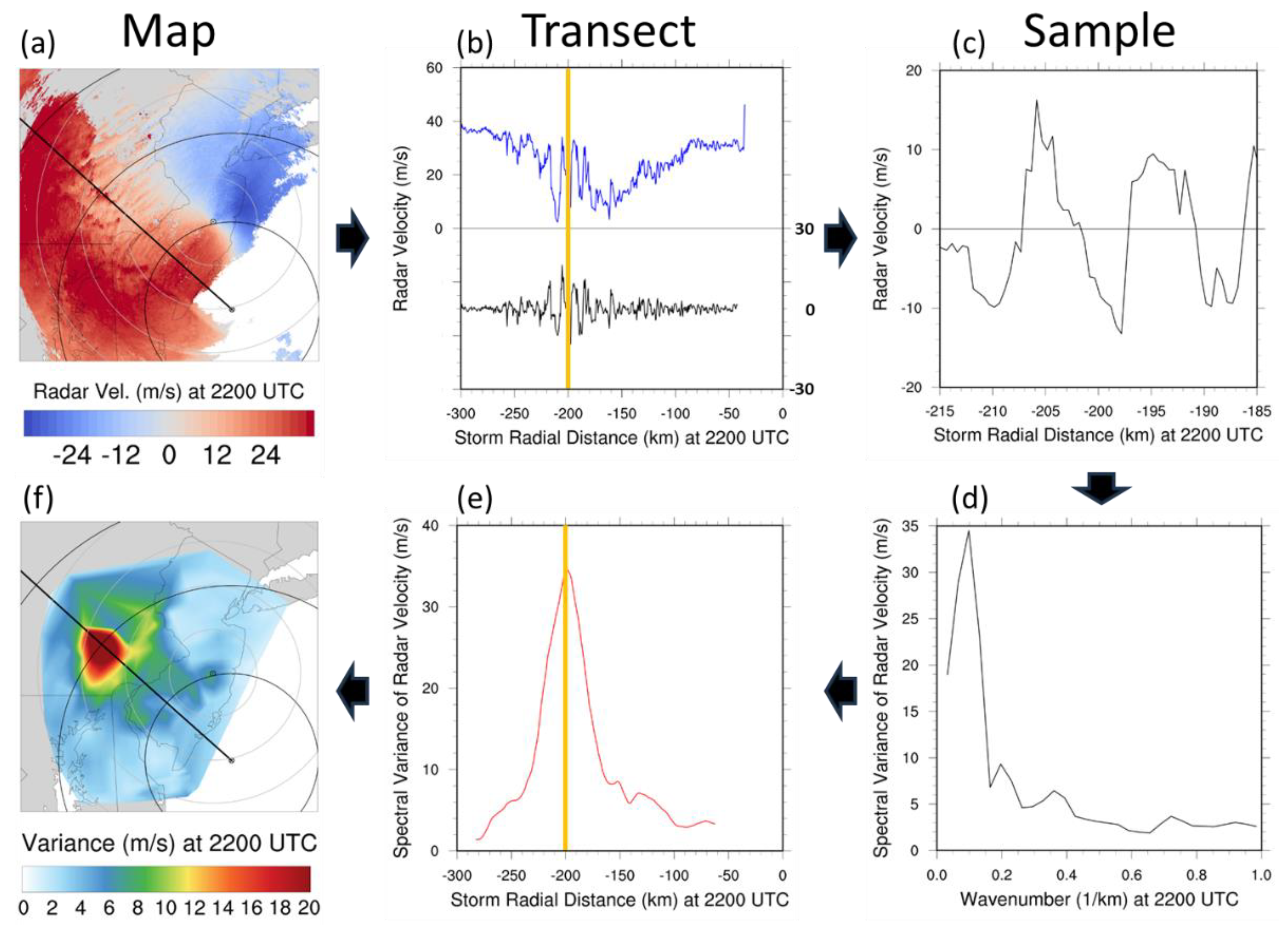
2.2. Methods
2.3. Metric Verification
3. Results
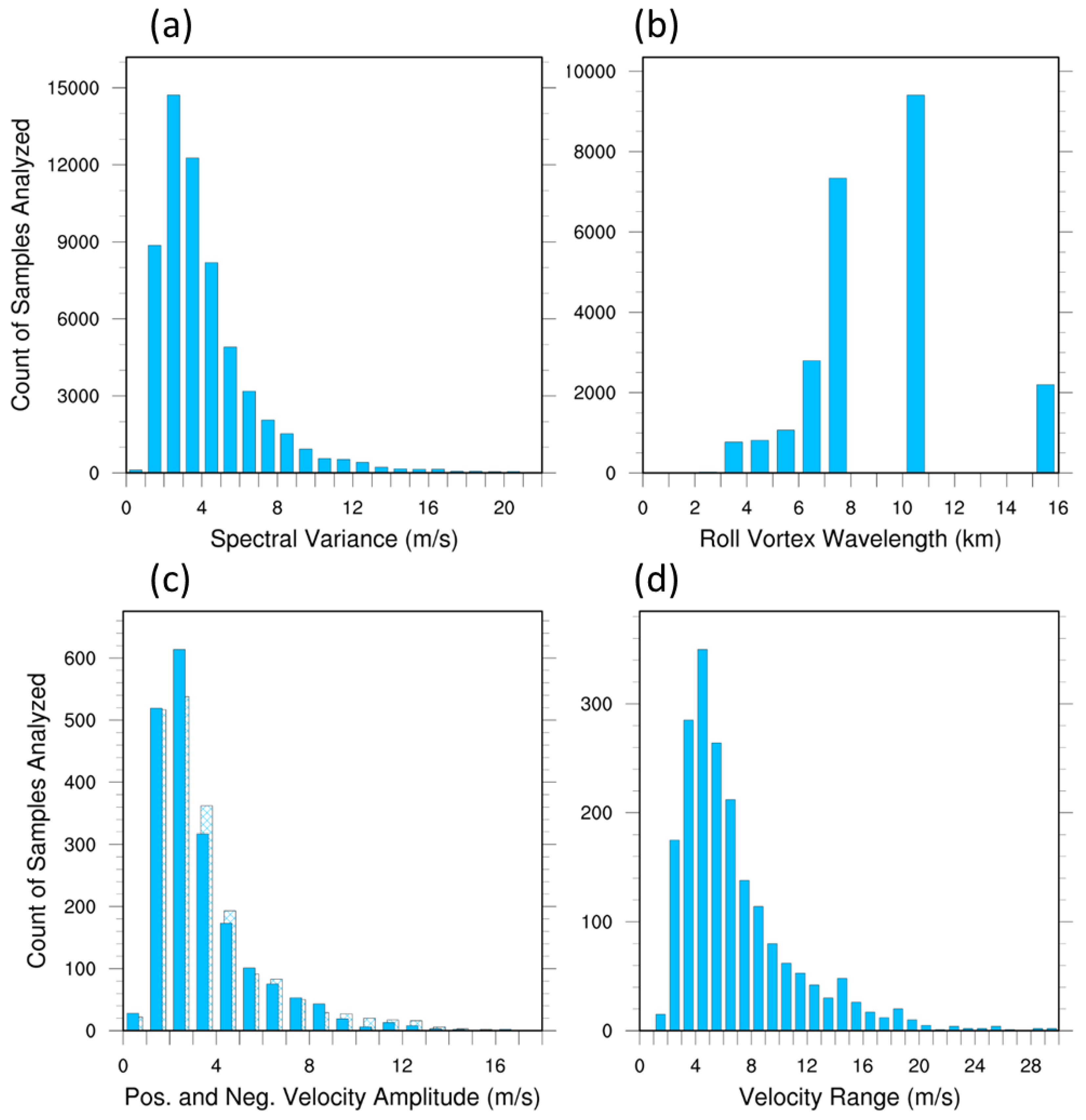
3.1. Roll Characterization Metrics
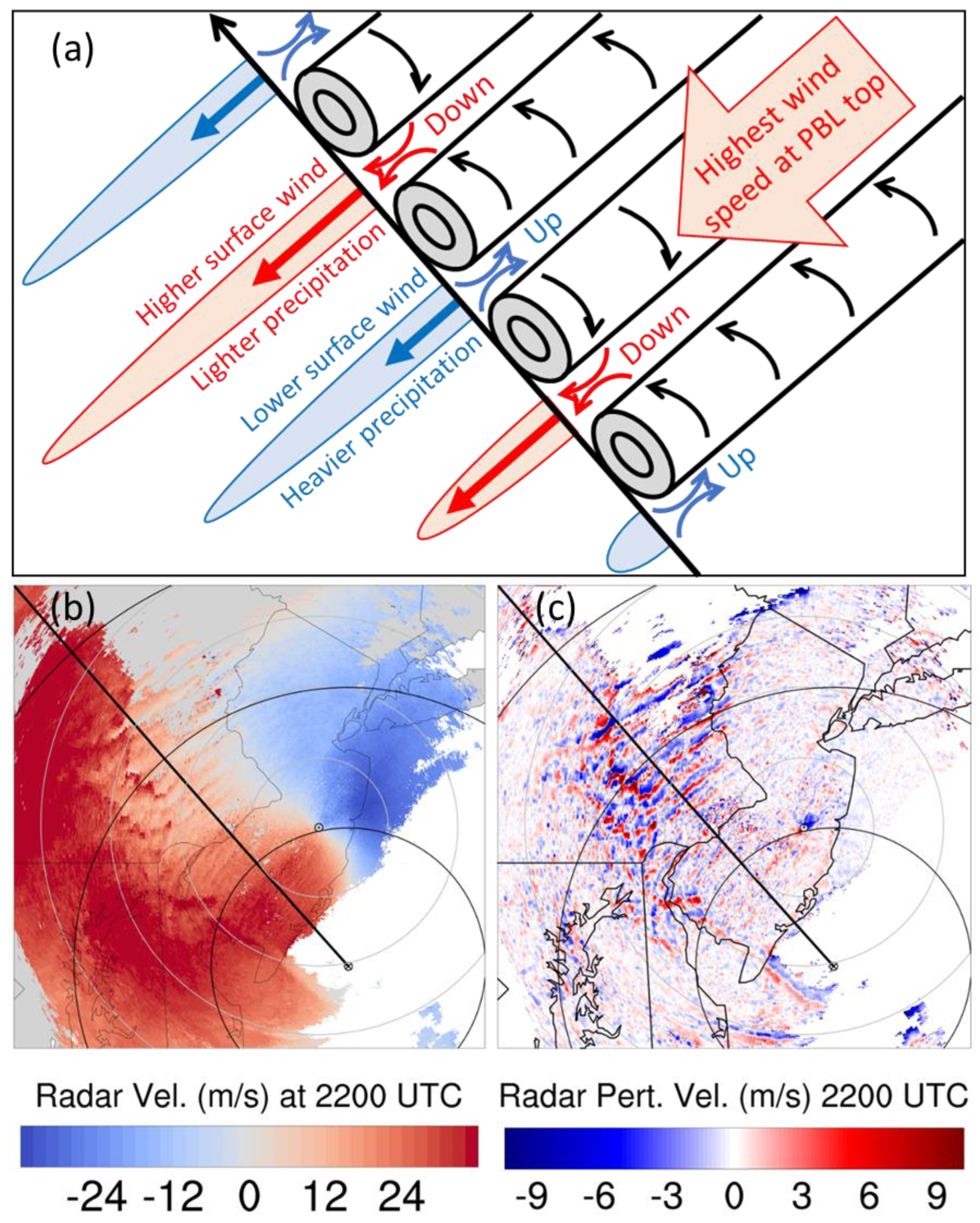
3.2. Reanalysis of Roll Association with Airstreams
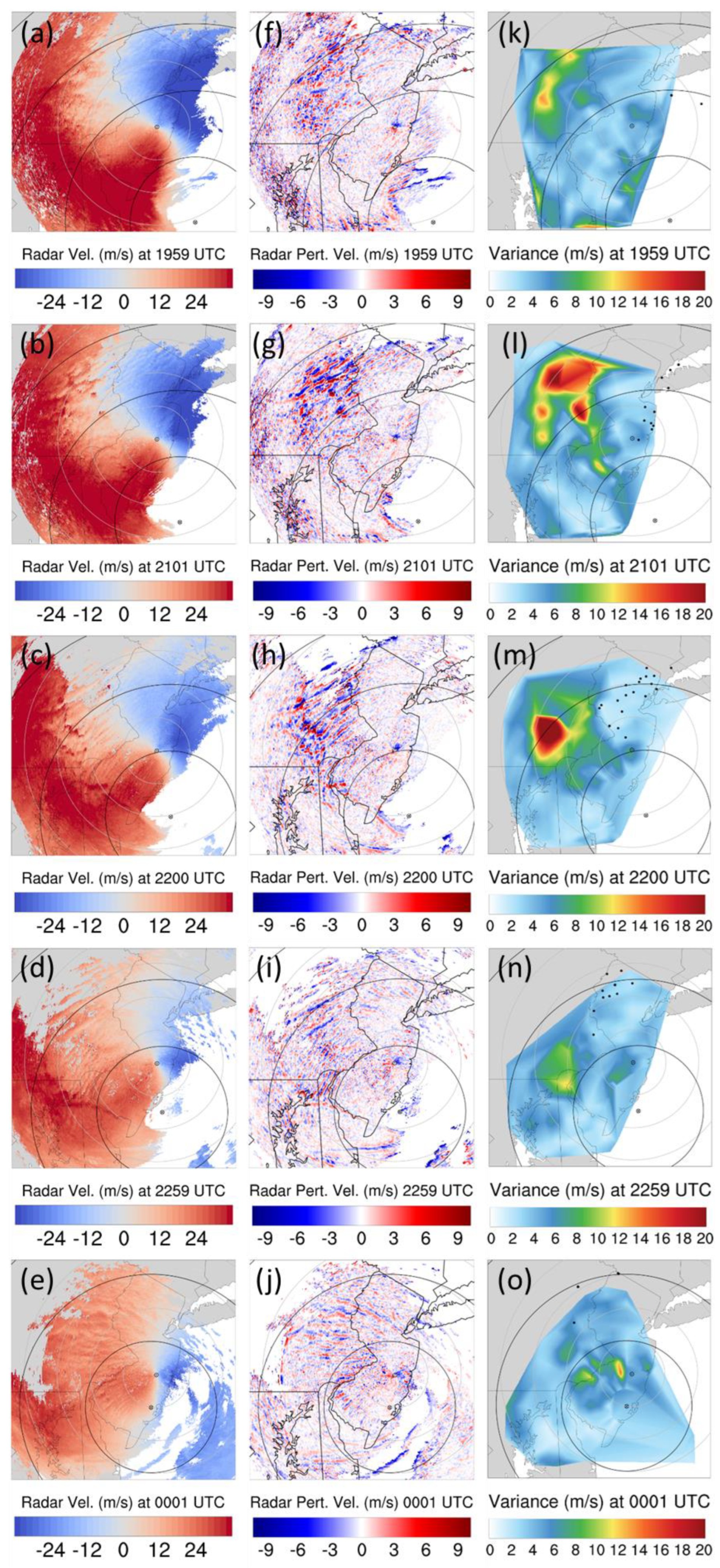
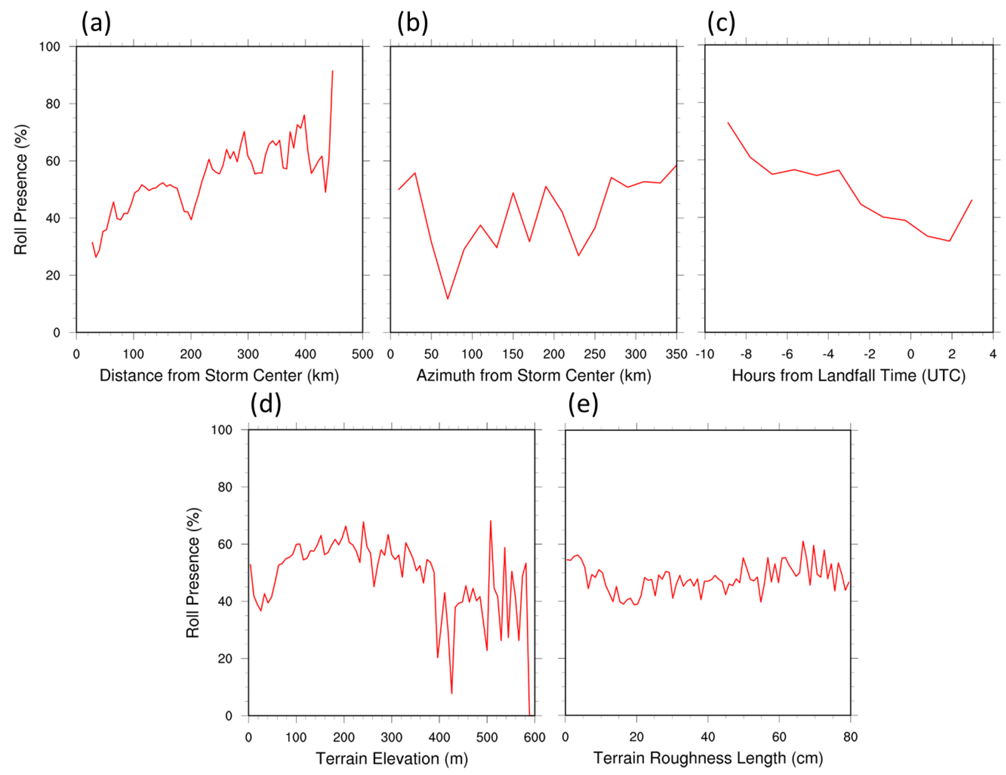
3.3. Roll Variation with Location, Time and Terrain
3.4. Roll Presence Analysis
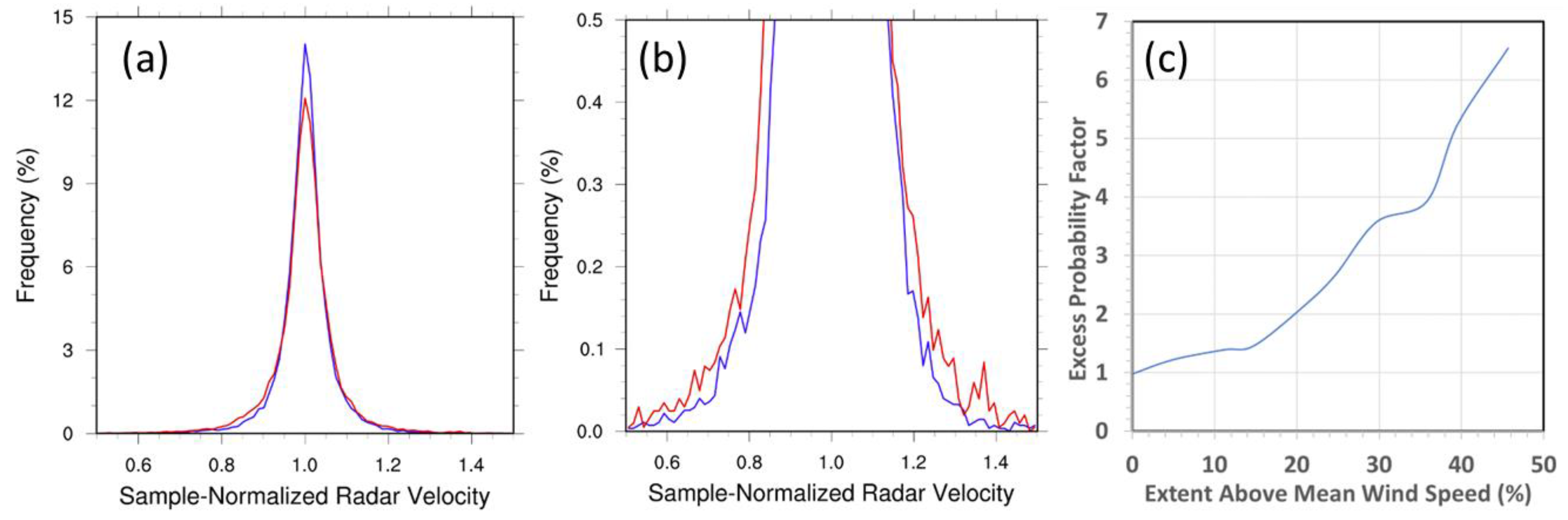
3.5. Wind Speed Enhancement Estimate
4. Discussion
4.1. Roll Presence Comparisons
4.2. Roll Wavelength Comparisons
4.3. Roll Intensity Comparisons
5. Conclusions
Funding
Data Availability Statement
Acknowledgments
Conflicts of Interest
Abbreviations
| TC | Tropical cyclone |
| SAR | Synthetic aperture radar |
| NDBC | National Data Buoy Center |
| NOAA | National Oceanic and Atmospheric Administration |
| WCT | Weather and Climate Toolkit |
| ESRI | Environmental Systems Research Institute |
| ASCII | American Standard Code for Information Interchange |
| UCAR | University Corporation for Atmospheric Research |
| NCAR | National Center of Atmospheric Research |
| NCL | NCAR Command Language |
| SV | Spectral variance |
| CCB | Cold conveyor belt |
| WRF | Weather Research and Forecasting |
| Probability density function | |
| RMW | Radius of maximum wind |
| SLD | Shear layer depth |
References
- Kuettner, J. (1959), The band structure of the atmosphere, Tellus, 11:3, 267-294. [CrossRef]
- Walter, B. A., and J. E. Overland (1984), Observations of longitudinal rolls in a near neutral atmosphere. Mon. Wea. Rev., 112, 200–208.
- Kelly, R. D. (1984), Horizontal roll and boundary-layer interrelationships observed over Lake Michigan. J. Atmos. Sci., 41, 1816–1826.
- Christian, T. W., and R. M. Wakimoto (1989), The relationship between radar reflectivities and clouds associated with horizontal roll convection on 8 August 1982. Mon. Wea. Rev., 117, 1530–1544.
- Etling, D., and R.A. Brown (1993), Roll vortices in the planetary boundary layer: A review. Boundary-Layer Meteorol., 65, 215–248. [CrossRef]
- Young, G. S., D. A. R. Kristovich, M. R. Hjelmfelt, and R. C. Foster (2002), Rolls, streets, waves, and more: A review of quasi-two-dimensional structures in the atmospheric boundary layer. Bull. Amer. Meteor. Soc., 83, 997–1002. [CrossRef]
- Wurman, J., and J. Winslow (1998), Intense sub-kilometer-scale boundary layer rolls observed in Hurricane Fran. Science, 280, 555-557. [CrossRef]
- Gall, R., J. Tuttle, and P. Hildebrand (1998), Small-scale spiral bands observed in Hurricanes Andrew, Hugo, and Erin. Mon. Wea. Rev., 126, 1749–1766.
- Ellis, R., and S. Businger (2010), Helical circulations in the typhoon boundary layer. J. Geophys. Res., 115, D06205.
- Morrison, I., S. Businger, F. Marks, P. Dodge, and J. A. Businger (2005), An observational case for the prevalence of roll vortices in the hurricane boundary layer. J. Atmos. Sci., 62, 2662-2673.
- Lorsolo, S., J. L. Schroeder, P. Dodge, and F. Marks Jr. (2008), An observational study of hurricane boundary layer small-scale coherent structures. Mon. Wea. Rev., 136, 2871–2893.
- Zhang, J. A., K. B. Katsaros, P. G. Black, S. Lehner, J. R. French, and W. M. Drennan (2008), Effects of roll vortices on turbulent fluxes in the hurricane boundary layer. Boundary-Layer Meteorol., 128,173–189. [CrossRef]
- Foster, R. C. (2013), Signature of large aspect ratio vortices in synthetic aperture radar images of tropical cyclones. Oceanography, 26, 58-67.
- Tang, J., J. A. Zhang, P. Chan, K. Hon, X. Lei1, and Y. Wang (2021), A direct aircraft observation of helical rolls in the tropical cyclone boundary layer. Scientific Reports, 11, 18771. [CrossRef]
- Schiavone, J.A., Gao, K., Robinson, D.A., Johnsen, P.J., Gerbush, M.R. (2021), Large roll vortices exhibited by Post-tropical Cyclone Sandy during landfall. Atmosphere, 12, 259. [CrossRef]
- Pantillon, F., B. Adler, U. Corsmeier, P. Knippertz, A. Wieser, and A. Hansen (2020), Formation of wind gusts in an extratropical cyclone in light of Doppler lidar observations and large-eddy simulations. Mon. Wea. Rev., 148, 353–375. [CrossRef]
- Gao, K., Ginis, I., Doyle, J. D., & Jin, Y. (2017). Effect of boundary layer roll vortices on the development of an axisymmetric tropical cyclone. Journal of the Atmospheric Sciences, 74(9), 2737-2759.
- Gao, K., & Ginis, I. (2016). On the equilibrium-state roll vortices and their effects in the hurricane boundary layer. Journal of the Atmospheric Sciences, 73(3), 1205-1222.
- Zhu, P. (2008), Simulation and parameterization of the turbulent transport in the hurricane boundary layer by large eddies, J. Geophys. Res., 113, D17104. [CrossRef]
- Wang, S., and Q. Jiang (2017), Impact of vertical wind shear on roll structure in idealized hurricane boundary layers. Atmos. Chem. Phys., 17, 3507–3524.
- Ito, J., T. Oizumi, and H. Niino (2017), Near-surface coherent structures explored by large eddy simulation of entire tropical cyclones. Sci Rep 7, 3798. [CrossRef]
- Mourad, P. D., and R. A. Brown (1990), Multiscale large eddy states in weakly stratified planetary boundary layers. J. Atmos. Sci., 47, 414–438. [CrossRef]
- Foster, R. C. (2005), Why rolls are prevalent in the hurricane boundary layer. J. Atmos. Sci., 62, 2647-2661.
- Nolan, D. S. (2005), Instabilities in hurricane-like boundary layers, Dynamics of Atmos. and Oceans, 40, 209-236. [CrossRef]
- Nakanishi, M., and H. Niino (2012), Large-eddy simulation of roll vortices in a hurricane boundary layer. J. Atmos. Sci., 69, 3558–3575. [CrossRef]
- Green, B. W., and F. Zhang (2015), Idealized large-eddy simulations of a tropical cyclone–like boundary layer. J. Atmos. Sci., 72, 1743–1764. [CrossRef]
- Li, X., Z. Pu, and Z. Gao (2021), Effects of roll vortices on the evolution of Hurricane Harvey during landfall. J. Atmos. Sci., 78, 1847-1867. [CrossRef]
- Momen, M., M. B. Parlange, and M. G. Giometto (2021). Scrambling and reorientation of classical atmospheric boundary layer turbulence in hurricane winds. Geophysical Res. Lett., 48, e2020GL091695. [CrossRef]
- Gao, K., and I. Ginis (2014), On the generation of roll vortices due to the inflection point instability of the hurricane boundary layer flow. J. Atmos. Sci., 71, 4292–4307. [CrossRef]
- Gao, K., and I. Ginis (2018), On the characteristics of linear-phase roll vortices under a moving hurricane boundary layer. J. Atmos. Sci., 75, 2589–2598. [CrossRef]
- Katsaros, K. B., Vachon, P. W., Black, P. G., Dodge, P. P., & Uhlhorn, E. W. (2000). Wind fields from SAR: Could they improve our understanding of storm dynamics? Johns Hopkins APL Technical Digest, 21(1), 86-93.
- Huang, L., Li, X., Liu, B., Zhang, J. A., Shen, D., Zhang, Z., & Yu, W. (2018). Tropical cyclone boundary layer rolls in synthetic aperture radar imagery. Journal of Geophysical Research: Oceans, 123(4), 2981-2996.
- Reppucci, A., Lehner, S., & Schulz-Stellenfleth, J. (2007, April). Tropical Cyclones Features Inferred from SAR Images. In ENVISAT Symposium 2007 (No. 2P1, pp. 1-6).
- NOAA National Weather Service (NWS) Radar Operations Center (1991), NOAA Next Generation Radar (NEXRAD) Level 2 Base Data. Products N0U, N0Q. NOAA National Centers for Environmental Information. https://www.ncei.noaa.gov/nexradinv/. Accessed 18 June, 2019.
- Halverson, J. B., & Rabenhorst, T. (2013). Hurricane Sandy: The science and impacts of a superstorm. Weatherwise, 66(2), 14-23.
- Comes, T., & Van de Walle, B. A. (2014). Measuring disaster resilience: The impact of Hurricane Sandy on critical infrastructure systems. ISCRAM, 11(May), 195-204.
- Mattingly, K. S., McLeod, J. T., Knox, J. A., Shepherd, J. M., & Mote, T. L. (2015). A climatological assessment of Greenland blocking conditions associated with the track of Hurricane Sandy and historical North Atlantic hurricanes. International Journal of Climatology, 35(5).
- Qian, W. H., Huang, J., & Du, J. (2016). Examination of Hurricane Sandy's (2012) structure and intensity evolution from full-field and anomaly-field analyses. Tellus A: Dynamic Meteorology and Oceanography, 68(1), 29029.
- Shin, J. H. (2019). Vortex spinup process in the extratropical transition of Hurricane Sandy (2012). Journal of the Atmospheric Sciences, 76(11), 3589-3610.
- Galarneau Jr, T. J., Davis, C. A., & Shapiro, M. A. (2013). Intensification of Hurricane Sandy (2012) through extratropical warm core seclusion. Monthly Weather Review, 141(12), 4296-4321.
- Martínez, P., Pérez, I. A., Sánchez, M. L., García, M. D. L. Á., & Pardo, N. (2021). Wind Speed Analysis of Hurricane Sandy. Atmosphere, 12(11), 1480.
- Zhu, T., & Weng, F. (2013). Hurricane Sandy warm-core structure observed from advanced Technology Microwave Sounder. Geophysical Research Letters, 40(12), 3325-3330.
- Shin, J. H., & Zhang, D. L. (2017). The impact of moist frontogenesis and tropopause undulation on the intensity, size, and structural changes of Hurricane Sandy (2012). Journal of the Atmospheric Sciences, 74(3), 893-913.
- Kowaleski, A. M., & Evans, J. L. (2018). Relationship between the track and structural evolution of Hurricane Sandy (2012) using a regional ensemble. Monthly Weather Review, 146(12), 4279-4302.
- Schiavone, J. A. (2023), Airstream association of large boundary layer rolls during extratropical transition of Post-tropical Cyclone Sandy (2012). Meteorology, 2, 368–386. [CrossRef]
- Blake, E. S., T. B. Kimberlain, R. J. Berg, J. P. Cangialosi, and J. L. Beven III (2013), Tropical Cyclone Report: Hurricane Sandy (AL182012). Tech. Rep. AL182012, NOAA/National Hurricane Center, 157 pp.
- Rutgers NJ Weather Network (2014), https://www.njweather.org/data/5min.
- NOAA National Data Buoy Center (2016), https://www.ndbc.noaa.gov/.
- NOAA Weather and Climate Toolkit (2021), https://www.ncdc.noaa.gov/wct/.
- The NCAR Command Language (Version 6.6.2) [Software]. (2019). Boulder, Colorado: UCAR/NCAR/CISL/TDD. [CrossRef]
- Landsea, C. W. & J. L. Franklin (2013). Atlantic hurricane database uncertainty and presentation of a new database format. Monthly Weather Review, 141, 3576-3592.

| Publication | Observation Method | Range (km) | Mean (km) |
| Wurman and Winslow, 1998 [7] | Mobile radar | − | ~0.6 |
| Gall et al., 1998 [8] | WSR-88D | − | ~10 |
| Katsaros et al., 2000 [31] | SAR | 4-6 | − |
| Morrison et al., 2005 [10] | WSR-88D | 0.5-3.0 | 1.45 |
| Foster, 2013 [13] | SAR | 10-20 | − |
| Reppucci et al., 2007 [33] | SAR | 0.6-2.0 | 0.99 |
| Lorsolo et al., 2008 [11] | WSR-88D | 0.2-1.4 | 0.5 |
| Zhang et al., 2008 [12] | Aircraft | − | 0.9 |
| Ellis and Businger, 2010 [9] | WSR-88D | 0.4-2.8 | 1.35 |
| Huang et al., 2018 [32] | SAR | 0.6-1.6 | − |
| Tang et al., 2021 [14] | Aircraft | 0.3-3.0 | − |
| Schiavone et al., 2021 [15] | WSR-88D | 5-14 | 8.6 |
| This work | WSR-88D | 3-15 | 8.7 |
Disclaimer/Publisher’s Note: The statements, opinions and data contained in all publications are solely those of the individual author(s) and contributor(s) and not of MDPI and/or the editor(s). MDPI and/or the editor(s) disclaim responsibility for any injury to people or property resulting from any ideas, methods, instructions or products referred to in the content. |
© 2025 by the authors. Licensee MDPI, Basel, Switzerland. This article is an open access article distributed under the terms and conditions of the Creative Commons Attribution (CC BY) license (http://creativecommons.org/licenses/by/4.0/).


