Submitted:
19 October 2025
Posted:
20 October 2025
You are already at the latest version
Abstract
Urban catchments are increasingly vulnerable to hydrologic extremes driven by land-use change and climate variability, challenging the traditional assumption of stationarity. This study develops a computational framework to assess the nonstationary behavior of peak flow, volume, and duration in an urban catchment in the Philippines using 38 years of daily flow records (June 1984–November 2022). Missing observations (~8% of the series) were reconstructed using multiple linear regression (MLR) and artificial neural networks (ANN) with four predictors: daily rainfall, antecedent rainfall, antecedent flow, and built-up area index. MLR with all predictors yielded the most accurate reconstructions. Nonstationarity was detected using the Mann-Kendall test, Sen’s slope estimator, Pettitt test, and variance change test. Flood events were extracted using block maxima (BM) and peak-over-threshold (POT) methods. BM-based results showed stationary peak flow and volume, while duration increased by 1.78 days/decade. POT analyses revealed nonstationarity across all dimensions, without significant shifts in variance. These findings demonstrate that methodological choices strongly influence nonstationary detection. The framework underscores the importance of reliable data reconstruction and robust statistical testing for nonstationary analysis of flood events. POT-based approaches more effectively capture evolving trends in peak flow, volume, and duration. This can be used in designing resilient infrastructure and flood risk management in urbanizing catchments.
Keywords:
hydrologic extremes
; nonstationarity
; urban catchment
; block maxima
; peak-over-threshold
1. Introduction
Climate change is subjecting river catchments to increasingly variable hydrologic extremes. In urban areas, these effects are intensified by rapid land-use change, which alters hydrologic response and heightens flood risk. Under such conditions, the long-standing assumption of stationarity in flow analysis, where the statistical properties of hydrologic records are considered constant over time, has become unreliable. Detecting and accounting for nonstationarity in flow records is therefore essential for developing accurate and robust flood risk assessments.
The need for accurate and robust flood risk assessment necessitates a thorough understanding of all flood characteristics, while ensuring that conclusions are drawn from multiple sets of flow data to ensure statistical validity [1]. Conventional analyses have historically focused on a single flood characteristic, typically peak flow. This approach, however, neglects the interconnected nature of other critical flood dimensions, specifically flood volume and duration. Previous studies have consistently demonstrated that these dimensions are frequently interdependent; for instance, peak flow and flood volume exhibit significant dependence structures [2,3,4]. Overlooking these crucial, multivariate relationships can lead to a substantial underestimation of flood hazard, particularly in environments that experience temporal shifts in their underlying statistical properties. Therefore, the prerequisite step of detecting and characterizing temporal changes across all relevant flood dimensions is vital for any subsequent statistical analysis.
The process of isolating extreme flood events is a crucial initial step in characterizing flood behavior and serves as a fundamental requirement before nonstationary detection. Event extraction methods, which directly influence the resulting time series, are typically categorized as the block maxima (BM) and peak-over-threshold (POT) approaches. Many studies recommended the joint use of BM and POT for comparison, as they offer complementary perspectives and often yield corresponding results [5,6]. While simple and widely applied [2,3], BM may overlook other extreme observations within the block. Moreover, it may underestimate design floods at longer return periods [7], leading to a growing preference for POT, which makes fuller use of available extreme events [6,8]. A key challenge in POT is threshold selection, as the choice strongly influences the statistical properties of the extracted series [9]. Studies have shown that in the application of POT in frequency analysis, as thresholds increase, uncertainty in scale and shape parameters rises, with particularly large uncertainty observed beyond the 98th percentile [9]. Percentile-based thresholds, as recommended by the WMO, are commonly adopted to balance data sufficiency and statistical stability [10]. The 95th percentile has been widely applied with promising results, including in the Mahanadi Basin [11] and in rainfall analyses with different percentile thresholds [12], where little difference was observed in design quantiles across thresholds of 95th–99.5th percentile. Other studies have sought to justify thresholds based on average event frequency, suggesting values ranging from 1.68 peaks per year [13] to around 3–8 events per year [8,14,15].
Nonstationarity in hydrologic time series has been increasingly documented. Studies have shown that flows in rivers and streams are influenced by multiple nonstationary drivers, including climate variability, land-use and land-cover changes, urbanization, and the construction of flood control structures [2,4,16]. As early as 2001, nonstationary detection had already been employed in 39 Polish rivers [17], while more recent studies attributed such behavior to rapid urbanization and population growth [12] and reservoir operations [18]. These findings raise an important methodological question of whether marginal distributions of each flood dimension in multivariate FFA should be modeled as stationary or nonstationary. Li et al. emphasized that even if variables such as peak flow and duration are independently and identically distributed, their marginals may remain stationary [16]. Incorrectly assuming nonstationarity, where it does not exist, or conversely assuming stationarity despite temporal changes, can bias model estimates and compromise flood risk management. Obeysekera and Salas similarly argued that designing flood structures under stationary assumptions, even in a changing environment, is no longer appropriate [19]. Reviews by Barbhuiya et al. further underline that nonstationary FFA is essential for addressing the combined impacts of climate change, land-use change, and human activity [20]. More recently, studies have begun integrating nonstationarity into the different flood dimensions in FFA [16,21].
While nonstationarity in flood records has already been documented in literature, much of this has focused primarily on peak flow, with comparatively less attention to other dimensions such as volume and duration. Where multiple dimensions are considered, analyses typically assume stationarity or do not explicitly test for temporal shifts in their distributions. In addition, while both BM and POT are established approaches for event selection, their influence on the detection of nonstationarity across different flood dimensions has received limited attention. This lack of integrated assessment constraints understanding how methodological choices affect the robustness of nonstationary detection, particularly in urban catchments where hydrologic extremes are shaped by both climate variability and rapid land-use change.
Motivated by this gap, this study investigates nonstationarity in multiple flood dimensions within an urban catchment in the Philippines. This employs both statistical and computational approaches. Missing values in the long-term flow dataset are reconstructed using multiple linear regression (MLR) and artificial neural networks (ANN), with predictors including rainfall, antecedent rainfall, antecedent flow, and a built-up area index. Peak flow, volume, and duration are the flood event dimensions that are extracted using both block maxima and peak-over-threshold methods. Each dimension is then subjected to trend, change-point, and variance shift tests to detect and characterize nonstationarity. Finally, the study evaluates how different event selection methods influence the detection and interpretation of nonstationary behavior.
By combining advanced statistical tests with data-driven models in data imputation, the study provides a comprehensive framework for analyzing nonstationary flood dimensions. The findings aim to enhance the accuracy and reliability of flood risk assessments in rapidly urbanizing environments, contributing to improved design standards and adaptive management strategies.
2. Materials and Methods
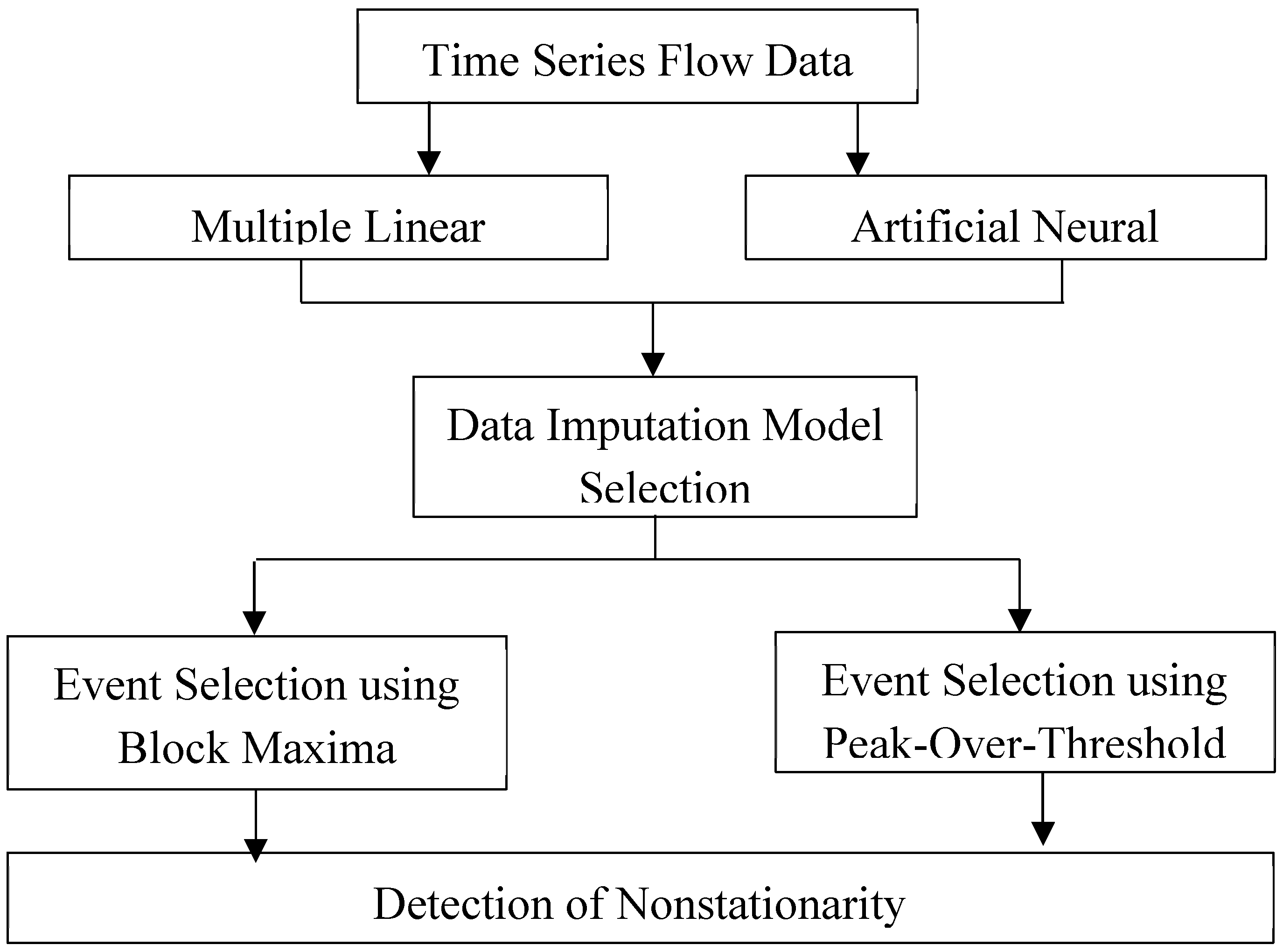
To carry out the objectives, the following methodological framework was used.
Figure 1.
Methodological Framework illustrating the key steps and components of the research design.
Figure 1.
Methodological Framework illustrating the key steps and components of the research design.
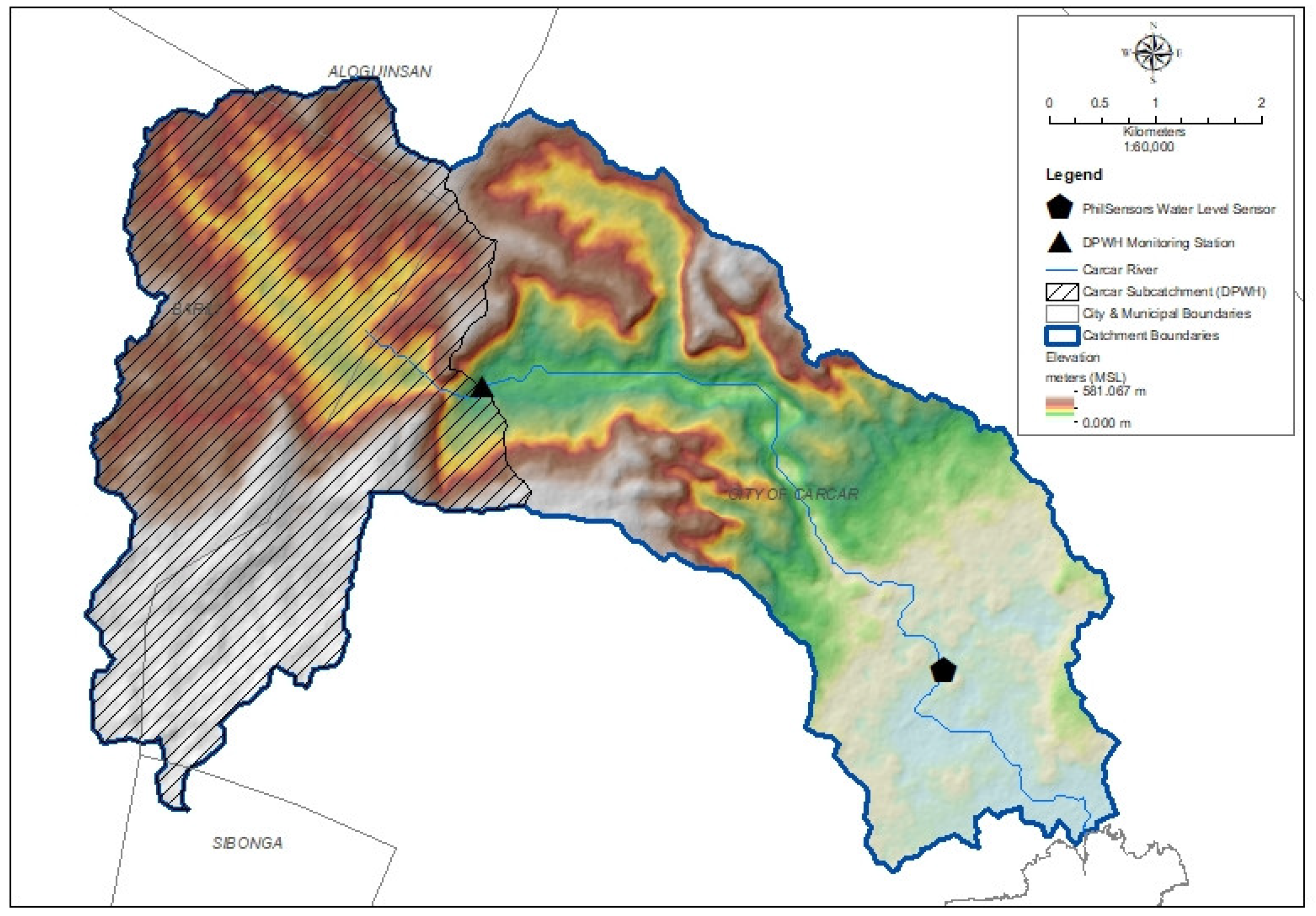
2.1. Study Area and Data Sources
The Carcar River catchment was selected as the case study site for detecting nonstationarity in flow data. Located in Carcar City, the southernmost city of Metro Cebu, Philippines, the catchment covers a total drainage area of approximately 38.58 km2 and drains towards the Cebu Strait. Its physiography is characterized by mountainous and hilly headwaters that transition into a narrow floodplain dominated by urban land uses. In recent years, the urbanized floodplain has experienced more frequent flooding, making Carcar River a representative example of small urban catchments where hydrologic extremes are intensifying due to combined climate and land-use pressures.
In response to these conditions, national agencies have installed monitoring instruments within the catchment. The Department of Public Works and Highways (DPWH) has maintained a flow observation site at 10°7′46″ N and 123°36′10″ E, recording daily flow data from 1984 to 2022. A complementary depth monitoring instrument is also installed downstream at Carcar Bridge under the supervision of PhilSensors.
For this study, the DPWH dataset was utilized, given its long-term record, which spans nearly four decades. The dataset includes daily peak flow observations along with monthly flow summaries, providing the basis for reconstructing missing values, extracting flood events, and assessing nonstationarity across key flood dimensions. The catchment area with the location of monitoring sites is presented in the map below.
Figure 2.
Carcar River Catchment showing locations of monitoring stations: DWPH flow observation site and PhilSensors water level sensor at Carcar Bridge. The map also illustrates the catchment boundary and elevation gradients, highlighting the transition from mountainous headwaters to the urbanized floodplain.
2.2. Data Processing
Historical flow datasets frequently contain missing values due to sensor malfunction, gaps in observation, or interruptions in data recording. The time series flow data obtained from DPWH contained approximately 8.26% missing values due to gaps in observation. These gaps are summarized in Table 1.
Traditional approaches for data imputation, such as deletion of incomplete entries or proxy substitution from nearby stations, may be suitable for short gaps (1–4 days) but become unreliable for extended periods of missing data (up to 382 days). More robust options for data imputation include mean substitution, interpolation, time series models, regression-based methods, and advanced techniques such as artificial neural networks (ANN).
Although data imputation is often overlooked in hydrologic analysis, it plays a crucial role in ensuring the accuracy and reliability of subsequent computations. Wu et al. demonstrated that model performance improves significantly when missing values in long datasets are properly reconstructed [22]. However, it should be noted that reconstructed data introduces an additional source of error that may propagate and affect further FFA results.
Given the extent of these missing records, multiple linear regression (MLR) and ANN imputation methods were evaluated. MLR remains a widely used technique because of its simplicity and interpretability. However, recent studies show that ANNs are increasingly adopted to address more complex, prolonged data gaps [23,24,25].
In this study, four predictors (daily rainfall, antecedent rainfall, antecedent flow, and built-up area index) were employed using both MLR and ANN models to impute missing flow values. This allowed the reconstruction of a more complete and consistent time series, thereby enabling more robust nonstationary analysis.
Daily rainfall data were obtained from the Philippine Atmospheric, Geophysical and Astronomical Services Administration (PAGASA). Built-up area indices were derived from Sentinel-2 satellite imagery (2016–2022) to quantify land use changes. Datasets (rainfall depth, flow, and built-up area index) from the years 2016 to 2022 have been extracted and have been subject to data imputation model generation.
Python-based algorithms were developed to train and evaluate both MLR- and ANN-based imputation models. The MLR algorithm utilizes the sklearn and pandas libraries. Consequently, the generated ANN algorithm utilizes the sklearn, pandas, and tensorflow libraries. The inclusion of ANN, in particular, was motivated by its ability to capture nonlinear dependencies between hydrologic variables, which linear regression models may not adequately represent. A certain percentage of data has been used to train the model, and the remaining data has been used for validation.
Model performance was assessed using the Pearson correlation coefficient, providing a quantitative measure of agreement between imputed and observed values. The model with the highest Pearson correlation coefficient has been selected for data imputation.
2.3. Event Selection for Flow Dimensions
Accurate extraction of flood events from continuous flow records is essential for reliable FFA. In this study, two widely used approaches were applied, BM and POT. BM was used to construct the annual maximum flow series by selecting the largest flow event in each year of record, while POT identified all independent exceedances above the 95th percentile of the flow observations. The choice of the 95th percentile was guided by existing literature, as it balances statistical stability and event representativeness while avoiding excessive uncertainty observed at higher thresholds.
For each extracted event, three flood dimensions were quantified: peak flow, defined as the maximum discharge during the event; flood volume, calculated as the integral of flow values above the baseflow over the event duration; and duration, measured as the continuous period from event onset until flow recession. The baseflow for each event was determined using the straight-line method. Python-based algorithms, developed using pandas, numpy and scipy libraries, were employed to automate the event extraction and reduce subjectivity, complementing manual calculations in Microsoft Excel.
2.4. Nonstationarity Detection
Detecting nonstationarity requires assessing whether the statistical properties of flow dimensions change over time. This study employed a suite of statistical tests to capture both gradual and abrupt changes. The Mann–Kendall test [26,27] was used to detect monotonic trends, while the Sen’s slope estimator [28] quantified their magnitude and direction. To identify abrupt shifts in the time series, the Pettitt test [29] was applied, and changes in variability were assessed using the variance change test [30] and Levene’s test [31].
All procedures were implemented through Python-based algorithms, ensuring reproducibility and computational efficiency. The integration of these complementary methods provides a comprehensive framework for detecting both gradual trends and sudden regime shifts in the flow record.
3. Results
3.1. Performance of Data Imputation Models
Initial attempts to predict daily peak flow using daily rainfall alone proved inadequate. This is likely due to the complex, non-linear relationship between rainfall and runoff, where factors such as impervious surfaces, drainage infrastructure, and antecedent conditions significantly influence peak flow response.
To improve model performance, antecedent rainfall, antecedent flow, and a built-up area index have been considered. Comparison of utilizing three predictors (excluding antecedent rainfall) and all four predictors is presented in Table 2. Various data train-test split (TTS) ratios were evaluated to identify the configuration yielding optimal predictive accuracy.
The results, summarized in Table 2, show that the MLR model consistently outperformed the ANN, with an R2 of 0.5684 when 5% of the data was used as test sets. For imputation of missing peak flow values across the dataset, the following MLR equation was used:
where is the daily peak flow, is daily rainfall, is the antecedent rainfall, is the antecedent peak flow, and is the built-up area index.
The complete daily flow time series, including imputed values, is presented in Figure 3, illustrating the effectiveness of the proposed model in reconstructing continuous hydrological records.
3.2. Event Extraction Using BM and POT Approaches
Flood dimensions were derived from the reconstructed series using both BM and POT approaches. Under the BM method, the annual maximum series was constructed, consisting of 38 peak flow events corresponding to the length of the dataset. From these events, associated volumes and durations were computed.
Using POT with a 95th percentile threshold, a larger number of extreme events was captured. This approach allows multiple events per year to be included, providing more detailed information on how flow extremes beyond the annual maxima. The choice of threshold in the POT method strongly influences the number and magnitude of the events captured, highlighting the method’s sensitivity.
The BM and POT approaches generated differing event sets, which can affect the detection and characterization of nonstationarity in flood dimensions. A comparison of the statistical properties of the resulting peak flow, volume, and duration for both methods is presented in Table 3.
3.3. Detection of Nonstationarity
Nonstationarity in the reconstructed flood series was evaluated using non-parametric trend and change point analyses. The results, summarized in Table 4, show the outcomes of the Mann–Kendall test, Sen’s slope, Pettitt test, and Levene test for peak flow, volume, and duration, using both BM and POT event extraction methods.
As evident in the values presented in Table 4, two event extraction methods yield different results. Moreover, the results of trend analyses of peak flow, volume, and duration over the study period are presented in Figure 4.
Analysis using the BM method indicated contrasting behavior among three flood dimensions. Peak flow and flood volume exhibited no significant monotonic trends, with Sen’s slope values close to zero and confidence intervals overlapping zero (e.g., peak flow Sen’s slope is 0.02, 95% confidence interval at -0.05 to 0.08 and p-value of 0.1). By contrast, flood duration showed a statistically significant increasing trend, averaging 0.35 days per decade (95% confidence interval at 0.10 to 070 and p-value of 0.05). Pettitt’s test detected a change point around 1998, suggesting a shift in hydrologic behavior during this period. However, variance tests indicated no significant changes in variability across the BM-derived series.
The POT method provided a different perspective, capturing multiple significant events per year. Here, all three flood dimensions, peak flow, volume, and duration, exhibited statistically significant nonstationary behavior. For peak flow, the Mann–Kendall test detected an upward trend, with Sen’s slope of approximately 0.25 (95% confidence interval at 0.12 to 0.40 and p-value < 0.01). Flood volume increased at a rate of (95% confidence interval at 0.05 to 0.55 and p-value <0.05), while duration rose by 0.45 days per decade (95% confidence interval at 0.15 to 0.75 and p-value < 0.05). Pettitt’s test identified change points in the mid-1990s to early 2000s across all three dimensions, aligning with periods of rapid urban development in Carcar City. Similar to the BM results, the variance tests did not confirm significant shifts in variability.
4. Discussion
4.1. Event Selection and Method Sensitivity
The results of this study underscore the importance of methodological choices in detecting nonstationarity in hydrologic extremes, particularly in urban catchments exposed to both climatic and land-use pressures. The analysis of imputation methods revealed that MLR with rainfall, antecedent rainfall, antecedent flow, and built-up area index as predictors provided the most reliable reconstruction of missing data. These finding highlights that even relatively simple statistical models can outperform more complex machine learning approaches, such as ANN, when the relationships between predictors and flow are largely linear. Similar observations were reported in studies wherein it was emphasized that careful selection of predictors may be more critical than model complexity in gap-filling time series [32,33]. In the context of nonstationarity detection, such methodological rigor in data imputation ensures that subsequent analyses are based on a consistent and trustworthy dataset.
Equally critical are the methodological decisions surrounding event selection. The comparison between BM and POT illustrates how different extraction approaches shape detection outcomes. BM, by focusing on the single largest event each year, provides a conservative and relatively stable representation of extremes but overlooks secondary events of hydrologic significance. POT, in contrast, captures multiple exceedances above the 95th percentile, offering richer information but also greater sensitivity to threshold choice. The adoption of the 95th percentile in this study reflects literature recommendations, balancing statistical stability and representativeness while avoiding the large uncertainties associated with thresholds exceeding the 98th percentile [5,8,9].
An additional challenge in tropical basins such as the Philippines lies in the strong seasonal influence of the El Niño Southern Oscillation (ENSO). During El Niño years, suppressed rainfall results in fewer or no events above the POT threshold, while La Niña years produce more frequent events. As a result, BM tends to mute these seasonal contrasts by selecting a single annual maximum, where POT amplifies them, making variance shifts and long-duration trends more apparent in La Niña-dominated years. This interplay between methodological choice and climatic forcing underscores the need for dual application: BM provides a conservative benchmark, while POT captures the broader distribution of flood extremes. Together, they offer a more comprehensive picture of nonstationary behavior in urbanized climate-sensitive catchments.
4.2. Trends and Effect Sizes in Flood Dimensions
Across the flow dimensions, Mann–Kendall results revealed significant trends in flood duration, while trends in peak flow and volume were less consistent between BM and POT. The Sen’s slope estimates quantify these effects, with duration showing the strongest changes, on the order of several days per decade, indicating that events are persisting longer even if peak intensities remain stable. Although some trends in peak flows were small in magnitude and associated with wide confidence intervals, the consistent signal in duration aligns with broader findings on flood persistence under climate and land-use change [12,34]. Effect sizes, therefore provide a critical distinction, even when p-values alone suggested weak or marginal trends, slope estimates revealed whether changes are practically meaningful for food risk assessment.
Uncertainty analysis further contextualizes these findings. Confidence intervals for Sen’s slope were narrowest in POT-derived peak flows, suggesting robust detection of moderate upward shifts, whereas BM-derived results often included zero, reflecting the loss of information from reduced sample size. Variance change tests supported these findings, with several periods showing significant increases in variability, an indication that floods are not only changing in central tendency but also in dispersion. This elevated variability poses challenges for infrastructure designed under fixed assumptions of flood behavior.
4.3. Abrupt Shifts and Nonstationary Drivers
The Pettitt test identified several significant change points, with major shifts aligning with periods of rapid urbanization. This temporal correspondence supports earlier findings by Villarini et al., who linked nonstationary behavior to land-use intensification [12]. In Carcar, abrupt shifts in duration suggest a compounded influence of both anthropogenic alterations and climatic variability. Importantly, these structural shifts emphasize that nonstationarity cannot be treated as a gradual phenomenon alone; sudden changes in watershed conditions can redefine baseline flood regimes within short periods.
4.4. Impact of Event Selection Method on Trend Analysis and Nonstationarity
The comparison of event extraction methods further emphasized the sensitivity of nonstationarity detection to data processing choices. Using BM, only flood duration exhibited significant nonstationary behavior, consistent with reports that flood persistence may be more susceptible to climatic and land-use drivers [2,35]. In contrast, POT-based analyses suggested nonstationarity across all three flow dimensions, confirming the view that POT provides richer information on extremes but is highly sensitive to threshold definition [36,37]. These results indicate that adopting multiple event extraction methods is beneficial for reducing methodological bias and ensuring robustness of hydrologic inference.
4.5. Implications for Practice
This study highlights key implications for urban flood risk management and hydrologic design. The detected increase in flood duration indicates that persistence, not only peak flows, must be considered in infrastructure planning. Divergences between BM- and POT-based estimates highlight the need for design standards that reflect methodological uncertainty in frequency analysis. The role of built-up area expansion in shaping flow further emphasizes the importance of integrating land-use planning with hydrologic assessments. Embedding nonstationary analysis into conventional practice will support the development of infrastructure and management strategies that remain resilient under climatic variability and rapid urbanization.
5. Conclusions
This study developed a comprehensive framework for detecting nonstationarity in multiple flood dimensions within an urban catchment in the Philippines. By integrating statistical methods (Mann–Kendall, Sen’s slope, Pettitt test, and variance tests) with data imputation techniques (Multiple Linear Regression and Artificial Neural Networks), the analysis addressed both data completeness and methodological sensitivity in evaluating hydrologic extremes. A notable finding was that MLR, using rainfall, antecedent rainfall, antecedent flow, and built-up area index as predictors, produced more reliable imputations than ANN. This highlights that predictor selection can be more critical than model complexity when reconstructing long-term hydrologic datasets.
The comparison of event extraction methods underscored how methodological choices shape nonstationarity detection. The Block Maxima approach offered conservative estimates of annual extremes, while the Peak-Over-Threshold method, using the 95th percentile, captured greater variability and was more sensitive to seasonal and interannual shifts, particularly under El Niño and La Niña conditions. The dual application of BM and POT illustrates the value of combining approaches. BM ensures robustness in long-term estimates, while POT captures short-term variability that is vital in urban flood risk assessment.
The novelty of this study lies in its integrated treatment of data imputation, event selection and nonstationarity testing within the context of a Philippine urban catchment, an approach rarely applied in local hydrologic studies. Practically, these findings stress the need to incorporate nonstationary frameworks into Philippine flood design standards, which remain grounded in stationary assumptions. Accounting for trends and shifts in flood peak, volume, and duration will strengthen the reliability of flood frequency analysis and help avoid under-designed flood protection systems.
Future research should extend this framework to other Philippine basins, integrate nonstationary flood frequency results with hydraulic and inundation modeling, and explore multivariate approaches to capture the joint behavior of flood dimensions. This study will not only advance scientific understanding but also provide a fundamental basis for climate-resilient planning and infrastructure design in rapidly urbanizing areas.
Author Contributions
Conceptualization, A.F.O., E.H. and G.T.; methodology, A.F.O.; software, A.F.O.; validation, A.F.O.; formal analysis, A.F.O., E.H. and G.T.; investigation, A.F.O., E.H. and G.T.; resources, A.F.O., E.H. and G.T.; data curation, A.F.O.; writing—original draft preparation, A.F.O.; writing—review and editing, A.F.O., E.H. and G.T.; visualization, A.F.O., E.H. and G.T.; supervision, E.H. and G.T.; project administration, A.F.O., E.H. and G.T.; funding acquisition, A.F.O., E.H. and G.T. All authors have read and agreed to the published version of the manuscript.
Funding
This research was funded by the Department of Science and Technology – Science Education Institute and Engineering Research and Development for Technology.
Acknowledgments
The rainfall data used in this study was acquired from the Philippine Atmospheric, Geophysical and Astronomical Services Administration.
Conflicts of Interest
The authors declare no conflicts of interest.
References
- Cunnane, C. Factors affecting choice of distribution for flood series. Hydrol. Sci. J. 1985, 30, 25–36. [Google Scholar] [CrossRef]
- Dong, N.D.; Agilan, V.; Jayakumar, K.V. Bivariate Flood Frequency Analysis of Nonstationary Flood Characteristics. J. Hydrol. Eng. 2019, 24. [Google Scholar] [CrossRef]
- Sraj, M.; Bezak, N.; Brilly, M. Bivariate flood frequency analysis using the copula function: a case study of the Litija station on the Sava River. Hydrol. Process. 2014, 29, 225–238. [Google Scholar] [CrossRef]
- Zhang, L.; Singh, V.P. Bivariate Flood Frequency Analysis Using the Copula Method. J. Hydrol. Eng. 2006, 11, 150–164. [Google Scholar] [CrossRef]
- Lang, M.; Ouarda, T.; Bobée, B. Towards operational guidelines for over-threshold modeling. J. Hydrol. 1999, 225, 103–117. [Google Scholar] [CrossRef]
- Langbein, W.B. Annual floods and the partial-duration flood series. Trans. Am. Geophys. Union 1949, 30, 879–881. [Google Scholar] [CrossRef]
- Kumar, M.; Sharif, M.; Ahmed, S. Flood estimation at Hathnikund Barrage, River Yamuna, India using the Peak-Over-Threshold method. ISH J. Hydraul. Eng. 2018, 26, 291–300. [Google Scholar] [CrossRef]
- Bezak, N.; Brilly, M.; Šraj, M. Comparison between the peaks-over-threshold method and the annual maximum method for flood frequency analysis. Hydrol. Sci. J. 2014, 59, 959–977. [Google Scholar] [CrossRef]
- Yue, Z.; Xiong, L.; Zha, X.; Liu, C.; Chen, J.; Liu, D. Impact of thresholds on nonstationary frequency analyses of peak over threshold extreme rainfall series in Pearl River Basin, China. Atmospheric Res. 2022, 276. [Google Scholar] [CrossRef]
- Data, C. Guidelines on analysis of extremes in a changing climate in support of informed decisions for adaptation. World Meteorological Organization 2009, 1500, 72. [Google Scholar]
- Guru, N.; & Jha, R. ; & Jha, R. International Journal of Innovative Research and Creative Technology 2015, 1(2), 220–223. [Google Scholar]
- Villarini, G.; Smith, J.A.; Ntelekos, A.A.; Schwarz, U. Annual maximum and peaks-over-threshold analyses of daily rainfall accumulations for Austria. J. Geophys. Res. 2011, 116. [Google Scholar] [CrossRef]
- Cunnane, C. A particular comparison of annual maxima and partial duration series methods of flood frequency prediction. J. Hydrol. 1973, 18, 257–271. [Google Scholar] [CrossRef]
- Pan, X.; Rahman, A.; Haddad, K.; Ouarda, T.B.; Sharma, A. Regional flood frequency analysis based on peaks-over-threshold approach: A case study for South-Eastern Australia. J. Hydrol. Reg. Stud. 2023, 47. [Google Scholar] [CrossRef]
- Beguería, S. Uncertainties in partial duration series modelling of extremes related to the choice of the threshold value. J. Hydrol. 2005, 303, 215–230. [Google Scholar] [CrossRef]
- Li, W.; Xiong, L.; Zhou, Y.; Yin, J.; Li, R.; Chen, J.; Liu, D. Nonstationary Seasonal Design Flood Estimation: Exploring Mixed Copulas for the Nonmonotonic Dependence between Peak Discharge and Timing. J. Hydrol. Eng. 2024, 29. [Google Scholar] [CrossRef]
- Strupczewski, W.; Singh, V.; Mitosek, H. Non-stationary approach to at-site flood frequency modelling. III. Flood analysis of Polish rivers. J. Hydrol. 2001, 248, 152–167. [Google Scholar] [CrossRef]
- Jiang, C.; Xiong, L.; Xu, C.; Guo, S. Bivariate frequency analysis of nonstationary low-flow series based on the time-varying copula. Hydrol. Process. 2014, 29, 1521–1534. [Google Scholar] [CrossRef]
- Obeysekera, J.; Salas, J.D. Quantifying the Uncertainty of Design Floods under Nonstationary Conditions. J. Hydrol. Eng. 2014, 19, 1438–1446. [Google Scholar] [CrossRef]
- Barbhuiya, S.; Ramadas, M.; Biswal, S.S. Nonstationary flood frequency analysis: review of methods and models. River, sediment and hydrological extremes: causes, impacts and management 2023, 271–288. [Google Scholar]
- Latif, S.; Mustafa, F. Bivariate joint distribution analysis of the flood characteristics under semiparametric copula distribution framework for the Kelantan River basin in Malaysia. J. Ocean Eng. Sci. 2021, 6, 128–145. [Google Scholar] [CrossRef]
- Wu, C.; Chau, K. Rainfall–runoff modeling using artificial neural network coupled with singular spectrum analysis. J. Hydrol. 2011, 399, 394–409. [Google Scholar] [CrossRef]
- Park, J.; Müller, J.; Arora, B.; Faybishenko, B.; Pastorello, G.; Varadharajan, C.; Sahu, R.; Agarwal, D. Long-term missing value imputation for time series data using deep neural networks. Neural Comput. Appl. 2022, 35, 1–21. [Google Scholar] [CrossRef]
- Cini, A.; Marisca, I.; & Alippi, C. Filling the gaps: Multivariate time series imputation by graph neural networks. arXiv:2021, 2108.00298.
- Bülte, C.; Kleinebrahm, M.; Yilmaz, H.Ü.; Gómez-Romero, J. Multivariate time series imputation for energy data using neural networks. Energy AI 2023, 13. [Google Scholar] [CrossRef]
- Mann, H. B. Nonparametric tests against trend. Econometrica 1945, 13(3), 245–259. [Google Scholar] [CrossRef]
- Marden, J.I.; Kendall, M.; Gibbons, J.D. Rank Correlation Methods (5th ed.). J. Am. Stat. Assoc. 1992, 87, 249. [Google Scholar] [CrossRef]
- Sen, P. K. Estimates of the regression coefficient based on Kendall’s tau. Journal of the American Statistical Association, 1968, 63(324), 1379–1389.
- Pettitt, A.N. A Non-Parametric Approach to the Change-Point Problem. J. R. Stat. Soc. Ser. C (Appl. Stat.) 1979, 28, 126–135. [Google Scholar] [CrossRef]
- von Neumann, J. Distribution of the ratio of the mean square successive difference to the variance. Annals of Mathematical Statistics 1941, 12(4), 367–395. [Google Scholar] [CrossRef]
- Levene, H. Robust tests for equality of variances. In I. Olkin (Ed.), Contributions to Probability and Statistics: Essays in Honor of Harold Hotelling; Stanford University Press, 1960; pp.
- Ribeiro, S.M.; Castro, C.L. Missing Data in Time Series: A Review of Imputation Methods and Case Study. Learn. Nonlinear Model. 2022, 20, 31–46. [Google Scholar] [CrossRef]
- Wu, R.; Hamshaw, S.D.; Yang, L.; Kincaid, D.W.; Etheridge, R.; Ghasemkhani, A. Data Imputation for Multivariate Time Series Sensor Data With Large Gaps of Missing Data. IEEE Sensors J. 2022, 22, 10671–10683. [Google Scholar] [CrossRef]
- Razmkhah, H.; Fararouie, A.; Ravari, A.R. Multivariate Flood Frequency Analysis Using Bivariate Copula Functions. Water Resour. Manag. 2022, 36, 729–743. [Google Scholar] [CrossRef]
- Zhang, T.; Wang, Y.; Wang, B.; Tan, S.; Feng, P. Nonstationary Flood Frequency Analysis Using Univariate and Bivariate Time-Varying Models Based on GAMLSS. Water 2018, 10, 819. [Google Scholar] [CrossRef]
- Ferreira, A.; & De Haan, L.; De Haan, L. On the block maxima method in extreme value theory: PWM estimators. The Annals of Statistics 2015, 276–298. [Google Scholar] [CrossRef]
- Kidson, R.; Richards, K.S. Flood frequency analysis: assumptions and alternatives. Prog. Phys. Geogr. Earth Environ. 2005, 29, 392–410. [Google Scholar] [CrossRef]
Figure 3.
Time series of daily peak flow showing observed values and imputed values generated using the four-predictor MLR model.
Figure 3.
Time series of daily peak flow showing observed values and imputed values generated using the four-predictor MLR model.
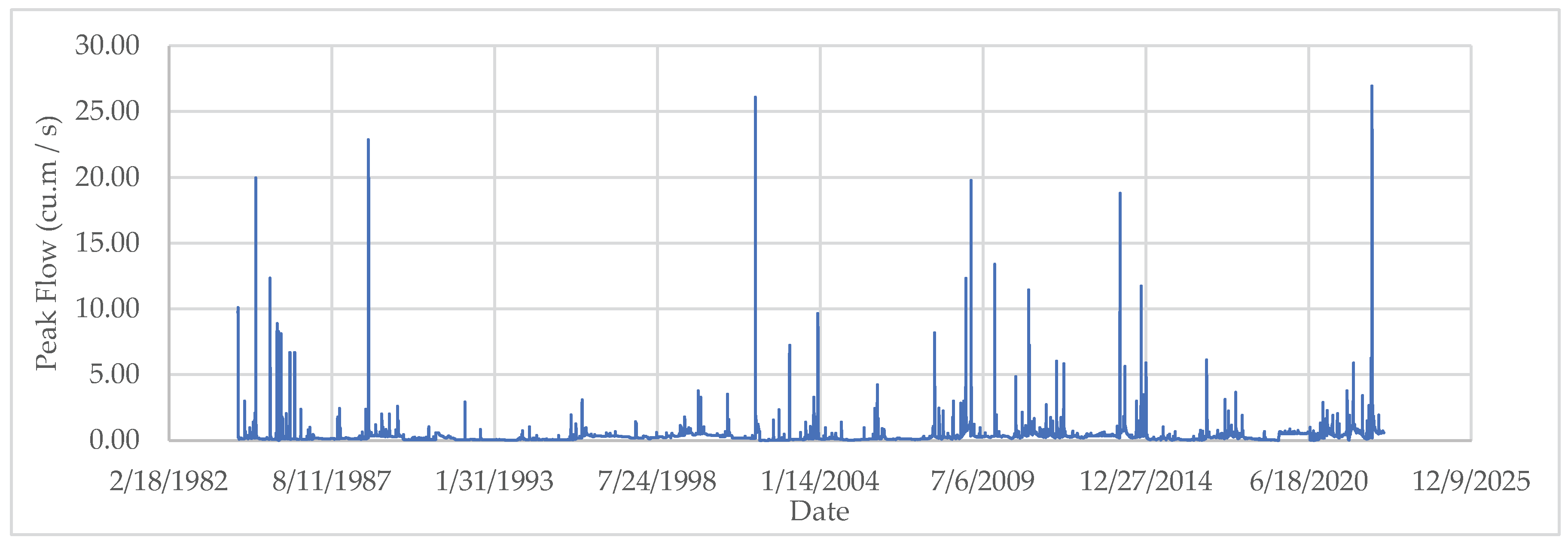
Figure 4.
Trend Analysis of flow peak, volume, and duration derived from BM (left) and POT (right) event extraction methods.
Figure 4.
Trend Analysis of flow peak, volume, and duration derived from BM (left) and POT (right) event extraction methods.
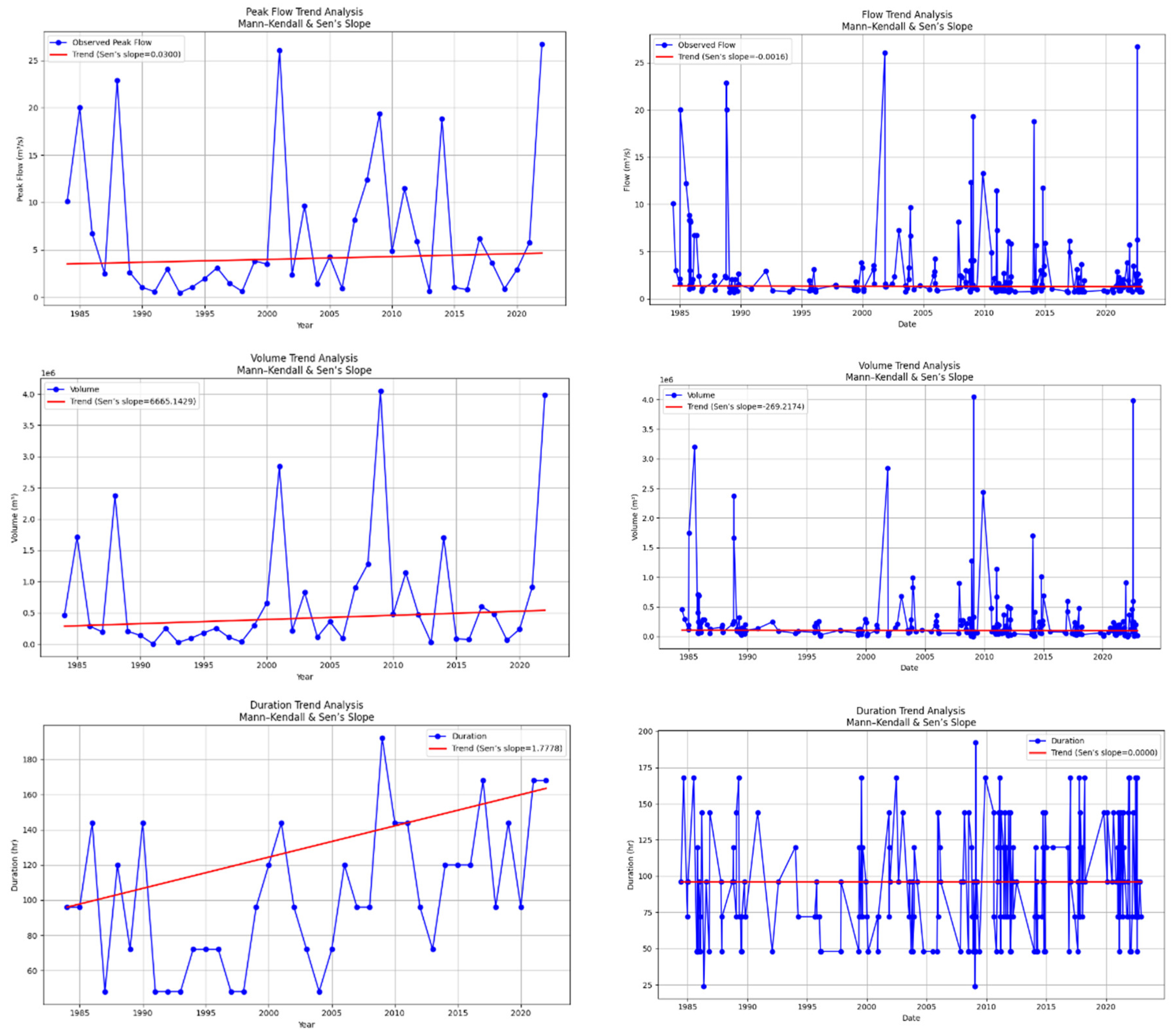

Table 1.
Data Gaps in the Flow Time Series Data of DPWH.
| Start | End | Number of Days |
|---|---|---|
| January 1, 1990 | December 31, 1990 | 365 days |
| November 21, 1993 | December 12, 1993 | 22 days |
| March 31, 2015 | 1 day | |
| January 1, 2013 | December 31. 2013 | 365 days |
| July 1, 2014 | July 4, 2014 | 4 days |
| July 1, 2015 | 1 day | |
| October 16, 2016 | October 30, 2016 | 15 days |
| June 17, 2019 | July 2, 2020 | 382 days |
| August 10, 2020 | August 11, 2020 | 2 days |
| August 15, 2020 | August 17, 2020 | 3 days |
Table 2.
Comparison of Performance of MLR and ANN Models.
| Train-Test Split | MLR | ANN | ||
|---|---|---|---|---|
| 3 predictors | 4 predictors | 3 predictors | 4 predictors | |
| 95-5 | 0.5638 | 0.5684 | 0.5616 | 0.5675 |
| 90-10 | 0.3887 | 0.3639 | 0.3916 | 0.4726 |
| 85-15 | 0.4254 | 0.3455 | 0.5406 | 0.3126 |
| 80-20 | 0.2287 | 0.2430 | 0.2262 | 0.2448 |
| 75-25 | 0.2358 | 0.2458 | 0.2340 | 0.2475 |
| 70-20 | 0.2319 | 0.2458 | 0.2316 | 0.2467 |
| 65-35 | 0.2354 | 0.2494 | 0.2348 | 0.2516 |
| 60-40 | 0.2287 | 0.2426 | 0.2281 | 0.2464 |
Table 3.
Statistical properties of peak flow, volume, and duration using BM and POT methods.
| Peak Flow | Volume | Duration | ||||
|---|---|---|---|---|---|---|
| BM | POT | BM | POT | BM | POT | |
| Minimum | 0.70 | 0.46 | 1,728 | 2,592 | 24.00 | 48.00 |
| Maximum | 26.70 | 26.70 | 4,045,248 | 4,045,248 | 192.00 | 192.00 |
| Mean | 2.83 | 6.64 | 268,698 | 721,611 | 91.56 | 102.15 |
| Standard Deviation | 4.09 | 7.54 | 545,692 | 1,014,071 | 37.35 | 39.98 |
| Coefficient of Variation | 1.44 | 1.13 | 2.03 | 1.41 | 0.41 | 0.39 |
Table 4.
Non-parametric trend and change point analyses results.
| Flow Dimensions | Peak Flow | Volume | Duration | |||
|---|---|---|---|---|---|---|
| Method | BM | POT | BM | POT | BM | POT |
| Mann–Kendall Test p-value | 0.5165 | 0.0143 | 0.3096 | 0.0036 | 0.0028 | 0.0075 |
| Kendall Tau | 0.0661 | -0.1066 | 0.1147 | -0.1268 | 0.3293 | 0.114 |
| Sen’s slope | 0.03 | -0.0016 | 6665.14 | -269.22 | 1.7778 | 0 |
| Pettitt Test p-value | 0.7168 | 0.0226 | 0.3058 | 0.027 | 0.0072 | 0.004 |
| Change Point | 1998 | 2010 | 1998 | 2008 | 2005 | 2009 |
| Levene p-value | 0.5382 | 0.0877 | 0.2077 | 0.7306 | 0.9291 | 0.5076 |
Disclaimer/Publisher’s Note: The statements, opinions and data contained in all publications are solely those of the individual author(s) and contributor(s) and not of MDPI and/or the editor(s). MDPI and/or the editor(s) disclaim responsibility for any injury to people or property resulting from any ideas, methods, instructions or products referred to in the content. |
© 2025 by the authors. Licensee MDPI, Basel, Switzerland. This article is an open access article distributed under the terms and conditions of the Creative Commons Attribution (CC BY) license (http://creativecommons.org/licenses/by/4.0/).
Copyright: This open access article is published under a Creative Commons CC BY 4.0 license, which permit the free download, distribution, and reuse, provided that the author and preprint are cited in any reuse.


