

Submitted:
17 October 2025
Posted:
20 October 2025
You are already at the latest version
Abstract
This paper presents three different approaches for generating points along the interaction diagram corresponding to design load effects, such as shear, bending moment, and axial force, to achieve optimal shear strength adequacy with the Australian bridge design standard AS 5100.5. The methodology targets the optimal shear condition by matching the design shear V∗ with the capacity ϕVu, V∗ = ϕVu, which represents achieving a load rating factor of unity within the specified tolerance limits. The first being a typical approach for generating points for two load effects is by increasing the M∗/V∗ ratio ηm in small increments from zero to a large value (theoretically infinity), and for each, to goal-seek the condition. The other approaches investigated are the use of increasing factored moment M∗ and the use of Monte Carlo simulation. A pretensioned bridge I-girder section reported in the literature was used in the study. The Monte Carlo simulation method was found
to be the simplest to program. It allows an interaction surface for the influence of three load effects for optimal shear adequacy to be obtained with minimal program coding. It can create 2-D interaction lines for various levels of shear adequacy k = V
∗/ϕVu for M∗ and V∗, and 3-D interaction surfaces for M∗, V∗ and N∗. The potential use of interaction diagrams was explored, and the advantages and limitations of using each method are presented. The interaction curves of two typical pretensioned concrete sections of a plank girder, one next to an end support and the other close to mid-span, were created to show the distinguishing features resulting from their reinforcment.
Keywords:
concrete
; shear
; design
; Monte Carlo Simulation
; interaction diagram
1. Introduction
In structural engineering, interaction diagrams are a valuable design tool, illustrating the failure envelope of a structural member caused by the interaction between load effects. The most common for analysis and design of concrete structures is the interaction between axial force N and bending moment M to cause failure of a reinforced concrete section [1]. Therefore, it is important to be able to create these diagrams with minimal programming effort to study the behavior of concrete structures and the effects of design requirements on the design of these structures.
The study focused on pretensioned concrete sections with straight tendons, establishing a clear basis for analysis. The proposed approaches, however, are equally applicable to reinforced and prestressed concrete sections with deflected tendons, underscoring their broader relevance. Three approaches were examined: (1) increasing moment–shear ratio, (2) increasing moment, and (3) Monte Carlo simulation. Among these, the Monte Carlo simulation approach was found to the easiest to program. To demonstrate this, 3-D interaction diagrams were created for the section of a pretensioned bridge section reported in the literature. In addition, contour plots of the interaction between shear and moment were created. The effect of axial force on the interaction was also investigated. Finally typical sections of a pretensioned concrete plank were used to show the distinguishing features of the diagrams resulted from their reinforcing.
2. Interaction Diagrams for Shear Adequacy Using MCFT-Based Strength of AS 5100.5
For bridge design to AS 5100.5 [2] and load rating to AS 5100.7 [3], the sought strength for a fictitious monotonic live load is not necessary as the non-iterative strength for load effects of the design or rating vehicle gives an accurate load rating factor for shear adequacy of the vehicle–bridge system under assessment [4,5,6]. is the ultimate shear strength , equaling , is the reduced ultimate shear strength, and is the capacity reduction factor for shear, equal to 0.7. The term “fictitious” is used here to describe a loading characteristic that is not consistent with the loading of the rating vehicle on the bridge. Consistency of strength and loading is a key feature of MCFT-based strength [7].
However, to accurately determine the allowable trailer load of a rating heavy vehicle with a platform trailer for the assessments of travel permit requests, a scaling factor of the trailer axle loads to give a load rating factor of unity is required [8,9]. The iterative solution procedure to achieve a load rating factor rating factor for shear requires repeated cycles of structural analysis of the vehicle–bridge system, each with a trial , using a non-linear solution search technique. Numerous trial girder sections, vehicle positions and scaling factors have to be considered.
A less rigorous approach is scaling the entire axle load of the vehicle on the bridge using a multiplying factor calculated from the sought strength based on an assumed fictitious monotonic loading. This method can be used to determine the allowable trailer load of a heavy vehicle with a platform trailer. However, its accuracy depends on the ability to correctly identify both the critical section and the position of the assessment vehicle at the critical loading stage. In addition, all axles of the vehicle on the bridge at the loading stage must be those of the trailer, not of the entire vehicle [10].
While interaction diagrams are not necessary for the design and load rating of structures for section shear, they are useful as a aid for selecting the size and reinforcement layout of sections of standard girders at the preliminary design stage. Standard precast prestressed concrete girders shown in Appendix D of AS 5100.5 are often used for bridge girders. Examples of design aids are the interaction diagrams provided for column sections in design handbooks [11,12].
They are also useful to study the effects of prescribed design requirements of design standards to modify the strength calculated using the MCFT equation by allowing their influence to be observed graphically. For example, the effect of limiting the design strength to in AS 5100.5 can be studied. Additionally, interaction diagrams, created for test conditions, using unfactored load effects and material properties, are useful to guide the design of laboratory testing to study the accuracy of proposed MCFT-based equations. For example, for a study to determine the accuracy of a proposed equation for shear strength, it is important to ensure that the test structure does not suffer premature yielding of the longitudinal reinforcement before the onset of section shear failure.
3. Determination of Ultimate Shear Strength
A Python [13] function CALC_SHEAR, common to all programs used in the study, was developed to calculate the reduced ultimate shear strength for a set of load effects, , and . It uses equations from AS 5100.5. The flow diagram for CALC_SHEAR is shown in Figure 1. The strength equation in CALC_SHEAR is suitable for sections of reinforced concrete and prestressed concrete beams with horizontal tendons. A flag variable is used in the main programs calling CALC_SHEAR to turn on and off the design requirement of , where is effective shear depth, for shear strength determination to allow the effect of the requirement to be studied. The variable is assigned in the main program to direct whether this requirement is to be considered. The value of is also set in the main program.
For section shear, the design requirements for the determination of ultimate shear strength to AS 5100.5 are:
- for calculating , where is the longitudinal strain in the concrete at mid-depth of the section;
- ; and
- .
The accuracy of the function CALC_SHEAR was checked using results for the analysis of a concrete section of a pretensioned concrete bridge girder with a cast in-situ concrete deck slab, referred to as Section 3, from a published article by Caprani and Melhem [14]. For this check, the equations used in CALC_SHEAR were changed to follow those of a previous version of AS 5100.5 without Amendment 2 of 2024 since the quoted article was published in 2019. Equation 8.2.3.3(1) for of this version is larger than that of the current version, which has an additional multiplying factor of 0.9. Also, Equation 8.2.1.7 of the previous version gave = MIN[ () ], which is different from the current = . Input values for the section are from the article. They did not provide the yield strength of the longitudinal reinforcement, and therefore the present study assumed it to be the same as their reported value = 400 MPa for fitments.
Geometric and material properties are listed in Table A1 of Appendix A.1, and the section is shown in Figure A1. The dimensions of the I-section are those of a standard precast I-girder of Type 3 shown in Figure D1(A) of AS 5100.5. Reinforcing steels were not shown in the figure as specific details of the prestressing strands were not reported by the authors. The stress in the prestressed reinforcement when the stress in the surrounding concrete is zero is assumed to be 0.7, where is the characteristic breaking strength, based on Clause 8.2.4.4 of AS 5100.5.
They reported an ultimate shear strength = 1767 kN for design shear = 1362 kN, and for = = 0.83 m. CALC_SHEAR gave the same value when the requirement of to be at least was not included, and the strength was found to be limited to as from the MCFT-based equation is greater than . Including the requirement, CALC_SHEAR gave = 1775 kN. for the section is 1.134 m. They reported a sought value = 1717 kN for = . Since CALC_SHEAR on its own is not able to determine the sought strength for the fictitious monotonic loading for , was determined for of 1717 kN. The value of was found to be = 1780 kN. CALC_SHEAR did not give equaling to it, suggesting that this reported value is not the converged solution for . Analysis using an Excel spreadsheet with its goal-seek feature gave a converged value of = 1782 kN, which was subsequently confirmed using CALC_SHEAR.
The results from CALC_SHEAR are summarized in Table 1. The design force in the longitudinal reinforcement is also presented in the table. At the design load level of 1362 kN, =2138 kN, which is less than = 4022 kN; this shows that the force from the design load effects is less than the force to cause yielding. The intersecting points of the loading line with = 0.83 with both the shear interaction curve and force interaction curve are shown in Figure 2. The force interaction curve is the load effects for where and . An assumption was made that the prestressed and non-prestressed steels provided are fully anchored at the section. The reduction factor for force in the longitudinal reinforcement, , is assumed to be 1.0 for this analysis. of 2170 kN with its concurrent of 1801 kNm are the load effects to cause yielding in the longitudinal steel.
For simplicity, instead of using the additional force (from shear) formulation of AS 5100.5, total force is used for checking force adequacy in the longitudinal steel. Total force in the steel is calculated as = + + , where is the additional force contribution from shear given by Equation 8.2.7(1) of AS 5100.5 equaling for a pretensioned section with undeflected tendons. This assumes that the force contribution from moment and axial force is , which is congruent to the practice in the USA [15]. It is also similar to that of AS 3600 [16] which uses + for the contribution from moment and shear respectively, where z is the lever arm between centroid forces acting on the section for bending. The equation for of this latest version of AS 3600 was changed, in Amendment 2, from the previous edition to be dependent on instead of . Vimonsatit, Wong and Mendis found that this change in AS 3600 was not suitable for load rating of structures, particularly those with shear deficiency [17].
The condition = for a fictitious loading is not useful for design and load-rating, where the requirement for shear adequacy is for the vehicle–bridge system under assessment. It is also not useful for laboratory testing to failure where the unfactored shear is sought to investigate the shear strength based on the MCFT-based equation. is the unfactored strength calculated using mean properties obtained from material testing. The analysis to seek described earlier in this section was carried out solely to enable the results from CALC_SHEAR to be checked against reported values from Caprani and Melhem [14].
Table 2 presented results for non-iterative and iterative values for Section 3. includes the factor of 0.9 added in Amendment 2 of AS 5100.5. The values for the sought conditions and are from analyses using the goal-seek feature of Excel. The values of and were both set to 0.7. Note that the requirements for (1) used for the calculation of to be greater or equal to , and (2) to be greater than were both included. The design check using the requirement of AS 5100.5 shows inadequacy for section shear as = 0.82. Since the characteristic strength of steel used is 400 MPa, this section was likely designed to an older version of the standard that used an empirically determined equation for strength, and therefore it is possible for the section to be understrength when checking it against requirements of the current standard. A check of the design for shear adequacy to the previous version of AS 5100.5 was not possible owing to missing the prestressing force required for the calculation. Force in the longitudinal reinforcement is adequate as = 1.11. of the section is 2816 kN. The intersecting points of the loading line for = 0.83 with both the shear interaction curve and longitudinal force interaction curve are shown in Figure 3.
In the calculation of , the contribution from moment, carried out with using the term in this study, AS 5100.5 does not require the to be at least for calculating this force component. In contrast, the contribution from shear uses calculated using and cot() with determined for the increased moment effect for . This suggests an inconsistency in the value of used for the calculation of the force contribution to from bending and shear for sections with .
4. Creation of 2-D Design Interaction Diagram
Two dimensional interaction diagrams are common as it is easy to visualize the interaction of two effects. This section describes three approaches for generating points on interaction diagrams for optimal shear adequacy ( = 1).
4.1. Increasing Moment-Shear Ratio,
Increasing the slope of the moment-shear ratio is the most common approach to create points to construct interaction diagrams. To locate the optimal-shear point for a known , the assumption of a fictitious monotonic loading of the load effects has to be made. To trace the entire interaction curve, the gradient of was progressively increased by changing its slope with the positive x-axis by varying it anti-clockwise from to in increments of . The slope for is infinity, and therefore was not used in the analysis. For each slope, an efficient non-linear goal-seek procedure consisting of two steps [8,18] was used, first seeking a bounding interval and then progressively halving it to achieve convergence. While other goal-seeking procedures can be used, they are likely not as stable as the one used in the study. Newton’s method has been used for solving nonlinear problems [19,20]. However, it requires initial guesses of load effects, and the procedure can be unstable if these guesses are not close to their values at convergence.
The goal-seek procedure was to determine equaling within prescribed tolerance limits. For each , the "seeking bound" step involved moving a fixed bounding interval of of 10 kN progressively by an increment of 10 kN in the increasing direction, starting from the lower bound value = 0 kN, until , which indicates that the bounding values have been found to start halving the bounding size. The "halving bound" step starts with the concurrent for the mid-level being calculated. The mid-point value is then checked to see whether convergence had been attained, using the criterion . A value of tolerance, 0.0001 was used in the study. If not achieved, one of the bounding values is replaced by to tighten the bounding size, and a new cycle of halving the bound is carried out until convergence was achieved.
The flow diagram in Figure 4 shows the "seeking bound" step of the program and Figure 5 the “halving bound” step to achieve convergence. Only the three input values axial force , shear and moment of CALC_SHEAR are shown in the flow diagram. The other input and output values are provided in Figure 1. The flow diagram shows only the output values to the file that was used for creating the plot of the interaction diagram. Other output values required for documenting the analysis, including read values from the input file, assigned , , , calculated , and determined , were written to another file.
Figure 6 presents the interaction diagrams illustrating optimal shear strength adequacy for the three different approaches. Figure 6(a) shows the diagram generated using the increasing approach. In comparison with the other two approaches, this method produces data points that are more widely spaced, especially as they move farther from the origin. Very fine incremental slope was necessary to create points closer together. Also, fewer points were created on the portion with a significant positive gradient slope. The effects of the requirements of AS 5100.5 for for calculating strength and can be seen on the left portion and that for can be seen on the right portion of the plot. The for obtained using a spreadsheet analysis with Excel is 531.8 kN, and this agrees well with the results from CALC_SHEAR, which show a leveling off of shear strength at approximately 531.7 kN.
4.2. Increasing Moment
After having established that the interaction curve from using the increasing approach in Section 4.1 that there were not more than one solution for strength over its range of moments, the study on the use of increasing moment value to generate optimum-shear points was carried out. This approach is not suitable where there are more than one convergence points for a given value. The procedure using increasing moment will not work as it can seek the lower point only if there are several points of adequacy with different . An example of an interaction diagram with two possible convergence points is that of column strength.
This approach uses the same two-step goal seek procedure of the increasing ratio approach. For each , the sought value of is obtained by varying only. The points generated are shown in Figure 6(b). The increasing moment approach provides points that are evenly spaced along the x-axis, making it easier to identify the cause of a sudden change in the slope of the interaction curve.
4.3. Monte Carlo Simulation
This approach uses the built-in random function of the NUMPY package in Python [13] to generate random numbers between two specified limits for every load effects. A random seed is not required for random number generation since the package can use a self-generated seed for its simulation. However, if a random seed value is not provided, the random numbers generated are not reproducible. While it is not necessary, a seed was used in the present study to ensure that the set of random values generated can be reproduced. A seed value of 2025 was used.
Figure 7 shows the flow diagram for the program. Two million () sets of random numbers for load effects were generated, with between 0 and 1900 kN, and between 0 and 10000 kNm. For each set of values, their concurrent was calculated using the CALC_SHEAR function. The same tolerance described in Section 4.1 was used to determine the closeness between and . The results for the set were printed to file for plotting only when this criterion was met. Of the 2 million sets generated, 155 were farmed and written to the output file for plotting. In this paper, the gathering of data points on the interaction diagrams is referred to as "farming".
Figure 6(c) shows the points presented as a scatter plot. It shows the randomness of the farmed numbers. Generating a larger number would have created a scatter plot with points closer together. The number 2 million was selected to enable the randomness of the points to be shown. Sorting the values was not required for the scatter plot. For a line plot, the points will have to be sorted in the order of increasing moment before plotting. The sorting is necessary to give a meaningful plot, with lines connecting adjacent points of increasing moment, rather than in the random order they were farmed. For a denser plot, the program can be changed to generate between 400 and 1400 kN, and between 0 and 8000 kNm.
5. Investigation of Localized Region of 2-D Interaction Diagram
While all three approaches can be used to investigate localized region of an interaction diagram, the increasing moment approach is the most suitable as it allows the moment to be increased in small step increments. In the present study, the cause of an abrupt change in slopes of the interaction curve was investigated by increasing from 1000 to 1300 kNm in steps of 5 kNm. Figure 8 shows the resulting scatter plot. The results from the analysis show the first noticeable slope change occurs at = 1260 kNm and = 1112 kN. The ratio of is 1.133 m, which is slightly less than the value of 1.142 m. To the right of this point, the points have ratio larger than this value. This shows that the change in slope is caused by the requirement of . The second slope change occurs at = 2380 kNm and it is caused by the change of sign of from negative to positive, and the third at = 2700 kNm by being no longer limiting .
Generating points for a region can also be carried out using the Monte Carlo approach. In this region, the ranges to use for the generation are 1080 to 1180 kN for , and 1000 to 3000 kNm for . Sorting the harvested data described in Section 4.3 is not necessary for the scatter diagram. However, it is useful for identifying the cause of the change in slopes. The increasing approach is the least suitable for this purpose as it is difficult to obtain uniformly spaced distributed points and can cause convergence problem if the slope in the approach is close to the positive gradient region of the curve with the point.
6. Creation of 3-D Design Interaction Diagram for Shear Adequacy
The use of Monte Carlo simulation made it easy to generate sets of load effects to study the interaction of more than two load effects. Figure 9 is a three dimensional scatter plot using the harvested points for the interaction of , and for optimal shear adequacy. The sign convention for is positive in tension. Of the 1 billion () set of numbers generated, 61660 sets which met the convergence criterion were farmed. The requirement of for calculating strength was not included in the analysis. The time taken is 121 minutes on a PC with an Intel Core i3-3220 GPu @3.30 GHz processor (Intel Corporation Santa Clara, CA, USA). The ranges of and used were as described in Section 4.3, and that for was for a range between 0 and 14000 kN. The effects of the requirements for and can be seen in Figure 9. For , the analysis gives 531.75 kN. To get for = 0 and = 531.75 kN, the required was 12640 kN, determined using the goal seek feature of an Excel spreadsheet. Above this value of , the interaction diagram is a straight line in the – plane with of approximately 532 kN.
To see the influence of the requirement when calculating strength, Figure 10 is the interaction diagram that meets the requirement. The reduced for optimal shear adequacy in the region of influence caused by the increased can be seen by comparing Figure 10 with Figure 9.
The open source application Octave [21] was used to create the plots. The figures can be rotated interactively on screen after producing them with the application thus enabling a closer examination of their features. Owing to the large number of points, the process of regenerating the plot with a change viewpoint was slow due to the limited computing configuration. This shortcoming can be overcome by generating fewer points or using a computer with a more powerful graphic processor.
6.1. 2-D Contour Diagram for = 0
An interaction diagram for optimal shear adequacy only provides information for combined load effects for optimal shear adequacy. To provide information for other levels of shear adequacy, additional interaction curves are required. A range of contour curves for the convergence criterion of , with k = 0.1–1.2, in steps of 0.1 are presented in Figure 11. The points were farmed using the Monte Carlo simulation. The program for the 2-D plot described in Section 4.3 was expanded to include the harvesting of points that met the convergence criteria of these contour curves. 10 millions () sets of points were generated for harvesting. The results for each contour curve were written to a separate output file for use with plotting. For example, the results for the curve with k = 0.2 for the convergence requirement was written to the file "surface02.dat".
Instead of using an interaction curve for optimal force adequacy of the longitudinal steel, the effect can be included by not harvesting those points with . The resulting contour plot with this included is shown in Figure 12. The interaction curve for force is also included to show that the curves terminate correctly. The results for plotting this are from the harvesting of the sets of load effects which satisfy the force adequacy convergence of , with = 0.0001. This was carried in the same program for harvesting the contour points for section shear adequacy since doing it separately gives the same results as the sets of points generated for harvesting are the same owing to using the same random generator seed. The terminating points are those with the shear adequacy of condition and optimal force adequacy in the longitudinal steel. The curve representing is also shown in the figure. A point on the intersection of the contour curve and the force interaction curve is a loading combination with optimal adequacy for both shear and force.
The interaction diagram for force can also be obtained using the increasing ratio approach but not the increasing moment approach owing to the vertical straight portion of the curve. This feature is caused by the expression "" of the Equation for being less than zero causing it to be set to zero. A negative value for this expression is not meaningful as the resistance term "" cannot be used to reduce the force components from the effects of and since they contribute to the force through structural behaviors different from shear. Note that is not strictly a factored force effect as part of it can be reduced by the resistance term "". With kN, m, and the shear contribution term set to zero, kN. Solving the equation gives kNm. The outputs from analysis gave = 3193 kNm for points on the vertical portion of the curve.
6.2. 3-D Contour Diagram for
The program for the 3-D plot described in Section 6 was expanded to enable points for interaction surfaces with different k values described earlier to be written to separate output files, where . The scatter plots are shown in Figure 13. The points on each surface are sufficiently close together to enable its shape to be visualized. The surface nearest to the origin is where k = 0.1 and that furthest k = 1.2.
7. Effects of Axial Force
Interaction curves for optimal shear adequacy for various values were created for the I-girder section. varies from −8000 kN to 8000 kN in increment of 2000 kN, and their 2-D interaction curves for are shown in Figure 14. is positive in tension. In total, 10 millions () sets of points were generated for harvesting. The diagram shows that a larger can be applied with decreasing . The compression effect is beneficial to increasing the moment that the section can carry before reaching its shear strength. The top portion of each curve shows the influence of the design requirement for not to exceed .
As previously discussed, it is possible to incorporate a strength check to ensure the longitudinal reinforcement remains adequate and does not yield. Figure 15 shows the interaction curves with points having removed. The generation was carried out using 10 million sets (), with ranging from 0 kN to 7000 kN and from 1200 kNm to 1270 kNm.
The plotted curves show that the regions that met both the requirement of and when = 4000 kN and above do not have points that met the force adequacy requirement. Additional interaction curves for various values of between = 0 kN and = 2000 kN were generated. Further increasing causes decreasing at convergence, which is shown in Figure 16. For clarity, these curves are not shown in Figure 15. The largest obtained is 3800 kN with a corresponding of 5 kNm and of 1028 kN, which explains the inability to harvest points for = 4000 kN.
Figure 16 is a plot of for a range of between −8000 to 3800 kN. For each of the value, the Monte Carlo Approach was used to harvest points which met the convergence criteria for both shear and force in the longitudinal steel. The point with the product of the two criteria closest to unity was selected for the plot. Key values of the plot are presented in Table 3. The curve for from −8000 (Point A) to 1200 (Point C) has of approximately 1120 kNm and approximately −28.8 . The noticeable change in slope at C is caused by the requirement of the standard for and that at D by shifting from a negative to a positive range causing a different equation to be used for the calculation of . The sharp change in slope at E is caused by the calculated using the MCFT-based equation not retricted by .
8. Effects of Reinforcement on Interaction Diagrams
In this section, the effects of the detail of reinforcement provided typically at a support section is compared with that of a span section. Typical sections of a pretensioned plank girder is used for the study. Geometric and material properties of these sections are listed in Table A2 of Appendix A.2. is assumed to be 0.7 . The section near mid-span is shown in Figure A2. The section has eight 15.2 mm diameter 7-wire prestressing ordinary strands in the flexural tension region, each with a sectional area of 143 . The section near the support is the same except the amount of ligatures is doubled by using N16@200 mm spacings and the number of bonded strands halved. For simplicity, the girder does not include the internal circular void usually provided to reduce self weight, and the profile of strands is horizontal, not deflected. Also, any tendons and non-prestressed reinforcement required in the compression region to control cracking were not shown as they are not required for shear strength calculation.
Two million () sets of points were generated for each section, and the harvested points for the contour curves were plotted in Figure 17 and Figure 18 for the support and span section respectively. Only points satisfying the force adequacy requirement were harvested. The optimal force adequacy interaction curve and the line for were also plotted. The shear depth of the support section is 330.74 mm and that of the span is 337.67 mm. The two figures were plotted using the same range of the values to enable comparisons to be made. As expected, the plots show that the detailing of the support is more suited for high shear, low moment regions near end supports and that of the span for high moment, low shear regions in the span. Both plots show that reducing the efficiency of the section for section shear by accepting a design with a lower k value allows the section to carry a larger moment before the onset of yielding of the longitudinal steels.
The interaction curves for k = 1.0, representing optimal shear adequacy, indicate that although the plotted points satisfy the condition using the strain calculated for an increased moment and shear , the sections would not meet the force adequacy requirement if this increased moment was also used to calculate the force component from flexure in that evaluation. This is because the corresponding points on the curve lie to the right of the optimal force adequacy curve.
9. Concluding Remarks
This paper presents three methods for generating design interaction diagrams aimed at optimizing the shear adequacy of concrete sections. Among these, the Monte Carlo method stands out for its simplicity, as it does not require a goal-seeking algorithm based on assumed fictitious loading. It is particularly effective for generating points along the interaction curve, making it useful for examining slope discontinuities introduced by specific design code requirements. Additionally, it facilitates the creation of contour plots and surfaces. The Monte Carlo approach also enables the analysis of interactions involving more than two influencing load effects on shear adequacy. However, while it can generate data for scenarios involving more than three interacting effects, visualizing such complex interactions graphically becomes challenging.
Although this study applied the Monte Carlo simulation approach to analyze the interaction of load effects for shear strength design, the method is equally applicable to investigating other structural behaviors. For instance, it can be used to assess the capacity of concrete columns subjected to combined axial and bending loads, supporting both design and experimental evaluations.
Author Contributions
Conceptualization, K.W.W. and V.V.; methodology, K.W.W. and V.V.; software, K.W.W.; validation, K.W.W. and V.V.; formal analysis, K.W.W. and V.V.; investigation, writing—original draft preparation K.W.W. and V.V.; writing—review and editing, K.W.W. and V.V.; visualization, K.W.W. and V.V.; All authors have read and agreed to the published version of the manuscript.
Funding
This research received no external funding.
Data Availability Statement
Data is contained within the article.
Conflicts of Interest
The authors declare no conflicts of interest.
Appendix A
Appendix A.1. I-girder
Figure A1.
Cross-section of the precast I-girder with cast in-situ deck slab
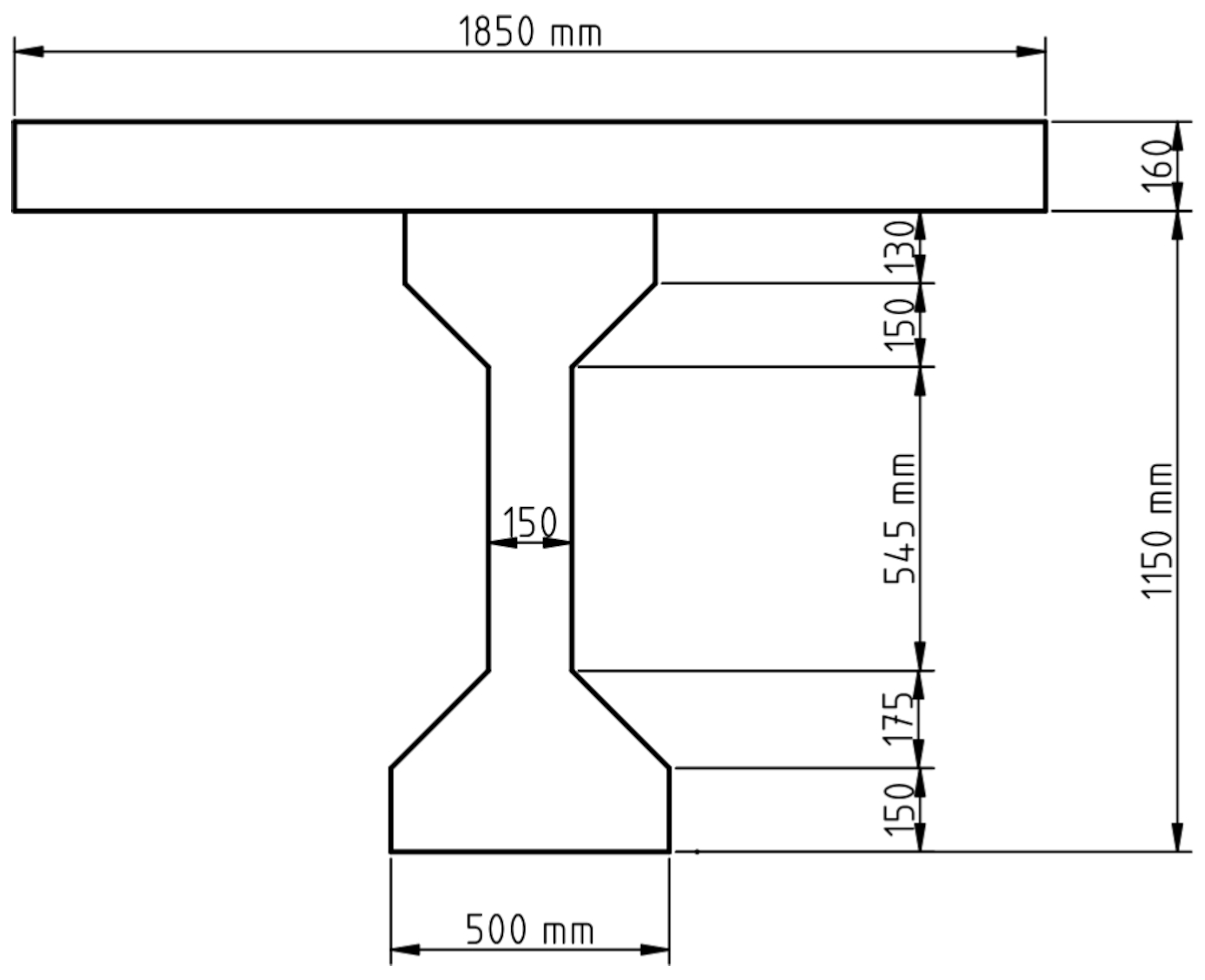
The table below summarizes the input values used in the program.

Table A1.
Input values.
| Section or material properties | Units | Values |
|---|---|---|
| D, overall depth of cross-section | mm | 1310 |
| d, effective depth of section | mm | 1260 |
| , effective width of section for shear | mm | 150 |
| , area of concrete on the tensile side of section | ||
| , area of longitudinal tensile reinforcement | 628 | |
| , area of tendons in the flexural tension zone | 2460 | |
| , area of shear reinforcement | 400 | |
| s, center to center spacing of fitments (stirrups) | mm | 225 |
| , characteristic compressive strength of concrete | MPa | 45 |
| , mean modulus elasticity of concrete | MPa | |
| , maximum nominal aggregate size | mm | 19 |
| , yield strength of fitments (stirrups) | MPa | 400 |
| , characteristic yield strength of longitudinal reinforcement | MPa | 400 |
| , modulus elasticity of reinforcement | MPa | |
| , modulus elasticity of tendons | MPa | |
| , characteristic breaking strength of tendons | MPa | 1870 |
| , yield strength of tendons | MPa | 1533 |
Appendix A.2. Plank
Figure A2 shows the cross-section of a section of the pretensioned bridge plank girder investigated.
Figure A2.
Cross-section of concrete pretensioned plank near mid-span.
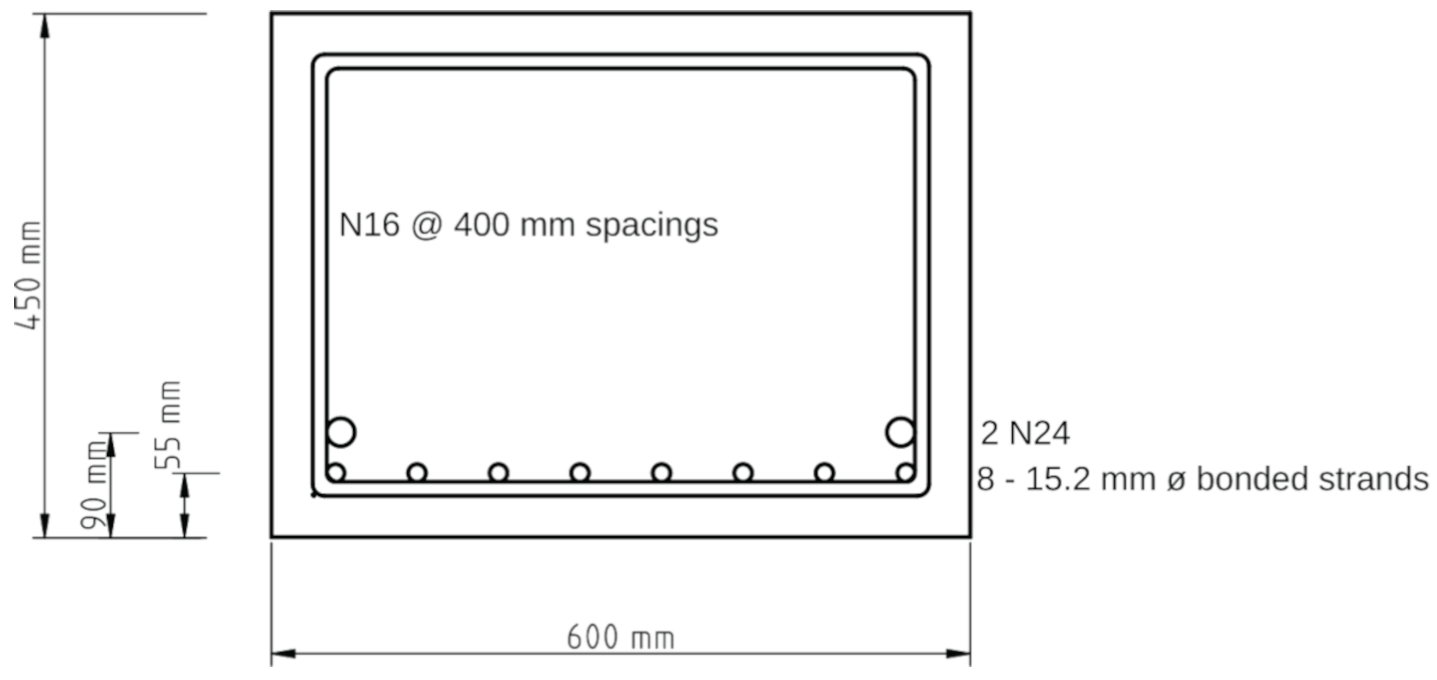
The table below summarizes the input values used in the program for the plank sections.
Table A2.
Input values.
| Section or material properties | Units | Values |
|---|---|---|
| D, overall depth of cross-section | mm | 450.00 |
| d, effective depth of section (support) | mm | 367.49 |
| d, effective depth of section (span) | mm | 375.19 |
| , effective width of section for shear | mm | 600.00 |
| , area of concrete on the tensile side of section | ||
| , area of longitudinal tensile reinforcement | 900.00 | |
| , area of tendons in the flexural tension zone (support) | 572.00 | |
| , area of tendons in the flexural tension zone (span) | 1144.00 | |
| , area of shear reinforcement | 400.00 | |
| s, center to center spacing of fitments (support) | mm | 200.00 |
| s, center to center spacing of fitments (span) | mm | 400.00 |
| , characteristic compressive strength of concrete | MPa | 50.00 |
| , mean modulus elasticity of concrete | MPa | |
| , maximum nominal aggregate size | mm | 19.00 |
| , yield strength of fitments (stirrups) | MPa | 500.00 |
| , characteristic yield strength of longitudinal reinforcement | MPa | 500.00 |
| , modulus elasticity of reinforcement | MPa | |
| , modulus elasticity of tendon | MPa | |
| , characteristic breaking strength of tendons | MPa | 1830.00 |
| , yield strength of tendons | MPa | 1501.00 |
References
- Warner, R.F.; Rangan, B.V.; Hall, A.S.; Faulkes, K.A. Concrete Structures, 3rd ed.; Publisher: Longman, Australia, 1988; pp. 673–678. [Google Scholar]
- AS 5100.5; Bridge Design Part 5: Concrete (with 2018 and 2024 amendments). Standards Australia: Sydney, NSW, Australia, 2017.
- AS 5100.7; Bridge Design Part 7: Bridge Assessment. Standards Australia: Sydney, NSW, Australia, 2017.
- Wong, K.W.; Vimonsatit, V. Determination of Shear Capacity for Load Rating of Concrete Bridges to AS 5100.7-2017. Infrastructures 2022, 7, 156. [Google Scholar] [CrossRef]
- Wong, K.W.; Vimonsatit, V. Determination of MCFT-based strength for Shear Load Rating of Concrete bridges—the Effects of Using Load-Dependent Strengths. In Proceedings of the Bridge Engineering Conference (BEI-2024), Las Vegas, USA, 22–25 July 2024; pp. 332–335. [Google Scholar]
- Wong, K.W.; Vimonsatit, V. Determination of MCFT-based Section Shear Strength for Load Rating and Design of Concrete Bridges—Is the Notion of Capacity Valid. In Proceedings of the Bridge Engineering Conference (BEI-2025), Paris, France, 21-24 July 2025; pp. 389–395. [Google Scholar]
- Holt, J.; Garcia, U.; Waters, S.; Monopolis, C.; Zhu, A.; Bayrak, O.; Powell, L.; Halbe, K.; Kumar, P.; Chavel, B. Concrete Bridge Shear Load Rating; Synthesis report; Federal Highway Administration, U.S. Department of Transport, 2018.
- Vimonsatit, V.; Wong, K.W. Bridge Management—Determination of Allowable Cartage Loads for the Movement of Heavy Vehicles with a Platform Trailer on Concrete Bridges to Satisfy MCFT-based Section Shear Strength. Infrastructures 2022, 9–236. [Google Scholar] [CrossRef]
- Vimonsatit, V; Wong, K.W. Prediction of Rating Factors for Managing Heavy Vehicles with a Platform Trailer on RC Bridges for Shear Adequacy — Inaccuracies from Using a Semi-Automatic Approach. In Proceedings of the Bridge Engineering Conference (BEI-2025), Paris, France, 21–24 July 2025; pp. 300–307. [Google Scholar]
- Vimonsatit, V; Wong, K.W. Bridge Assessment Using MCFT—Determination of Load Multiplying Factors for Optimal Shear Adequacy. In Proceedings of the Bridge Engineering Conference (BEI-2024), Las Vegas, USA, 25 July 2024; pp. 88–93. [Google Scholar]
- Reynolds, C.E.; Steedman, J.C. Reinforced Concrete Designer’s Handbook, 9th ed.; Publisher: Viewpoint Publication, U.K, 1981; pp. 404–439. [Google Scholar]
- Cement and Concrete Association of Australia. Concrete Design Handbook, 4th ed.; Publisher: Cement and Concrete Association of Australia and Standards Australia, 1995; pp. 6.6–6.29. [Google Scholar]
- Python. Available online: https://python.org (accessed on 14 August 2025).
- Caprani, C.C.; Melhem, M.M. On the use of MCFT per AS 5100.5 for the assessment of shear capacities of existing structures. Aust.J. Struct. Eng. 2019, 21(1), 53–63. [Google Scholar] [CrossRef]
- AASHTO. AASHTO LFRD Bridge Design Specifications, 10th ed.; American Association of Bridge Highway and Transportation Officials: Washington, DC, USA, 2024. [Google Scholar]
- AS 3600; Concrete Structures (with 2018 and 2021 Amendments). Standards Australia: Sydney, NSW, Australia, 2018.
- Vimonsatit, V.; Wong, K.W.; Mendis, P.A. Increase in Longitudinal Steel Reinforcement to Account for Shear in RC Beam Design to AS 3600. Proceedings of Concrete 2023 Conference, Perth, Australia, 10–13 September 2023; Available online: https://ciaconference.com.au/concrete2023/content.html (accessed on 23 September 2024).
- Warner, R.F.; Lambert, J.H. Moment-Curvature Time Relations for Reinforced Concrete Beams; IABSE Publication, 1974; Volume 34-I, pp. 181–203. [Google Scholar]
- Harrison, H.B. Interactive Nonlinear Structural Analysis. J. Struct. Div., ASCE July, 1976, 102-7, 1353–1364. [Google Scholar] [CrossRef]
- Wong, K.W.; Haritos, N.; Mansell, D.S. The Elastic Behaviour of Imperfect Slender Frames. In Proceedings of the Metal Structures Conference, Brisbane, Australia, 18-20 May 1983; pp. 80–86. [Google Scholar]
- Octave. Available online: https://octave.org/ (accessed on 18 September 2025).
Figure 1.
Flow diagram of Python function CALC_SHEAR
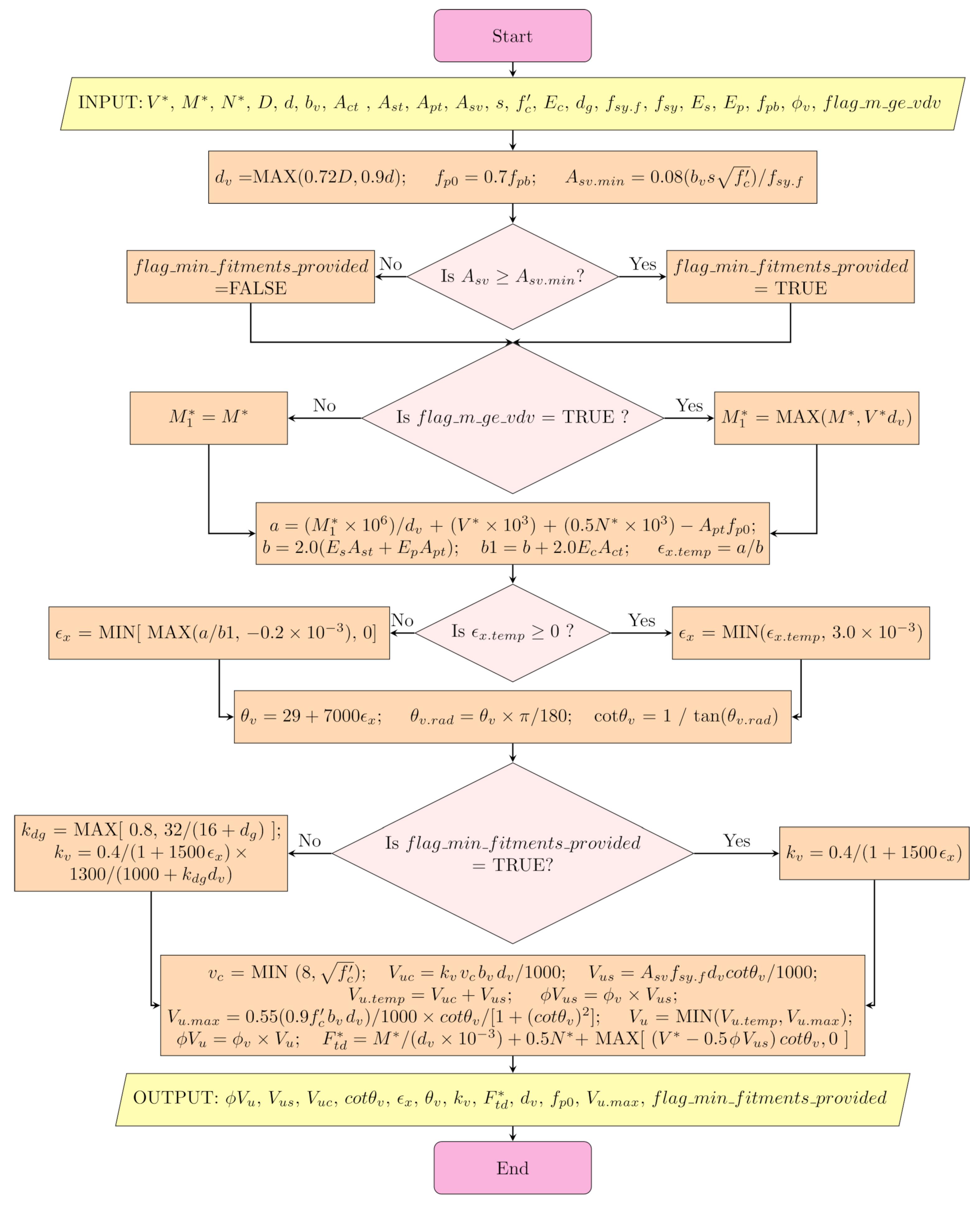
Figure 2.
Interaction curves for unreduced strength.
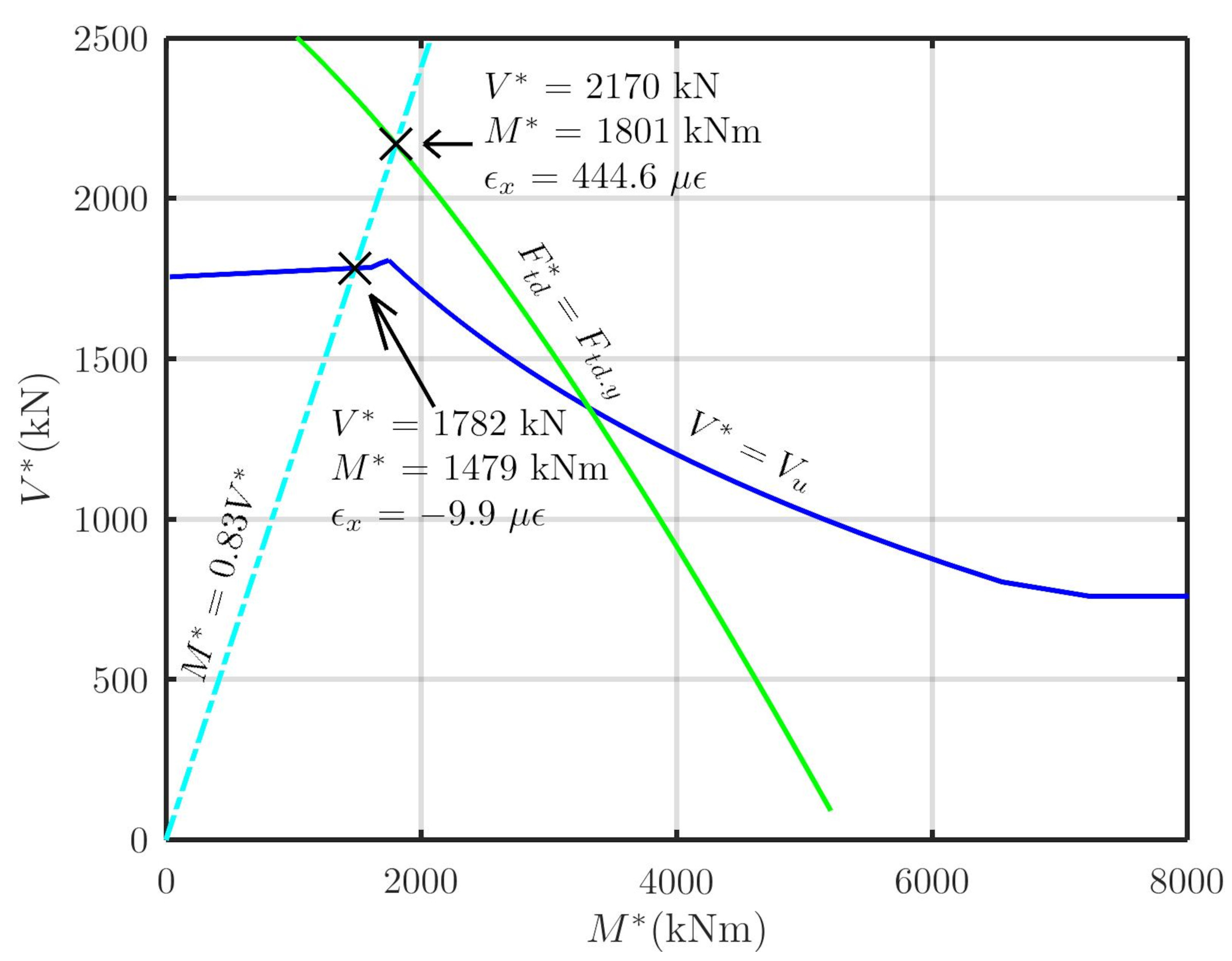
Figure 3.
Interaction curves for reduced strength.
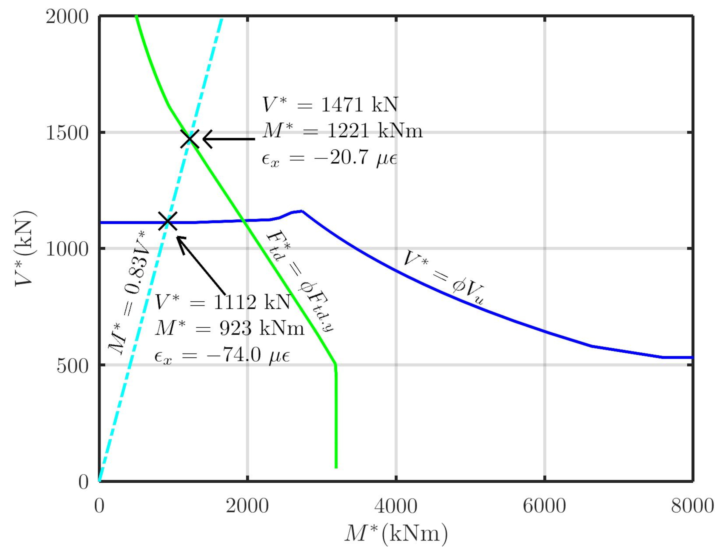
Figure 4.
Flow diagram of the “Seeking Bound” step of the goal-seek procedure.
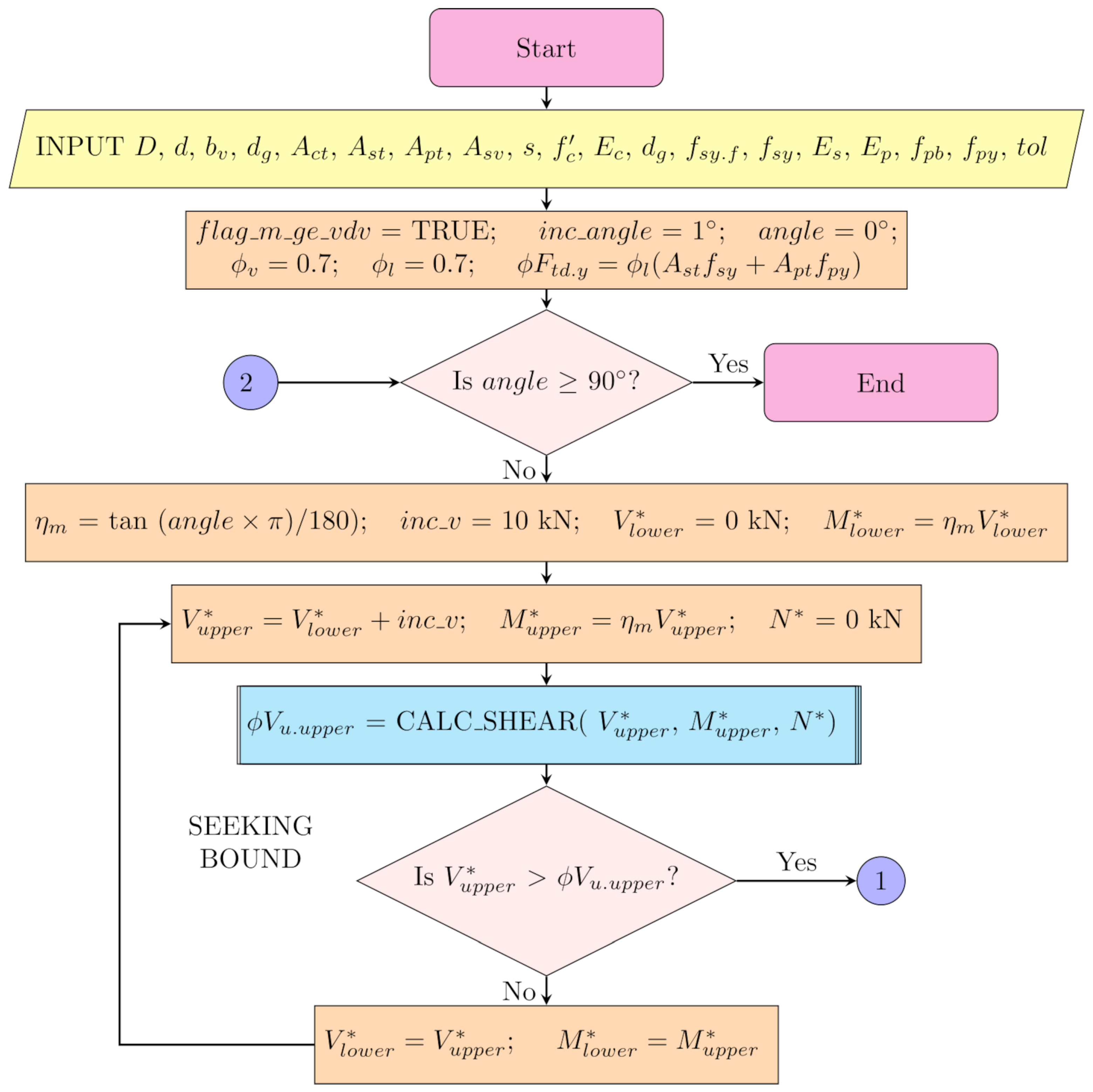
Figure 5.
Flow diagram of the “Halving Bound” step of the goal-seek procedure.
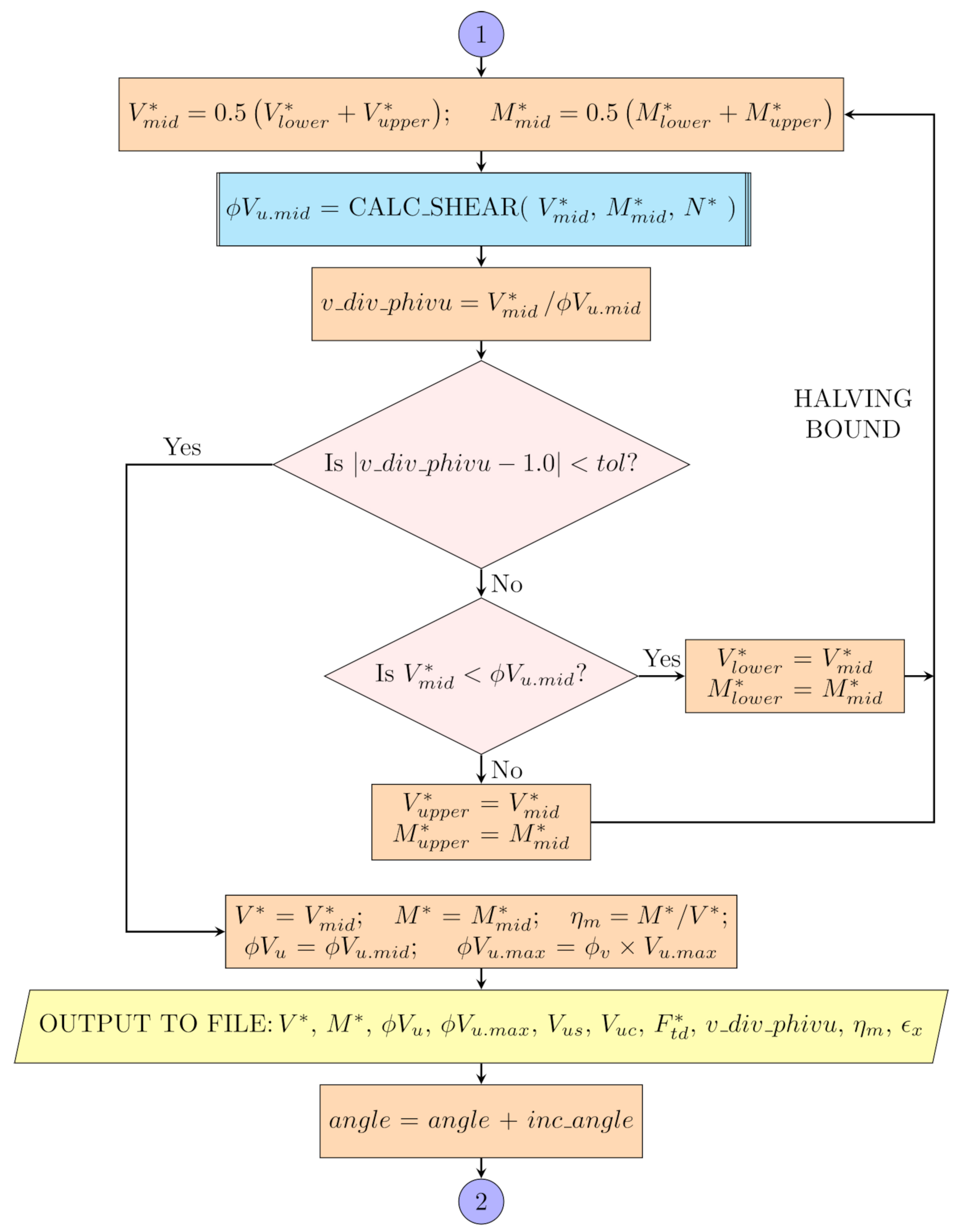
Figure 6.
Design interaction diagrams for from the three approaches.
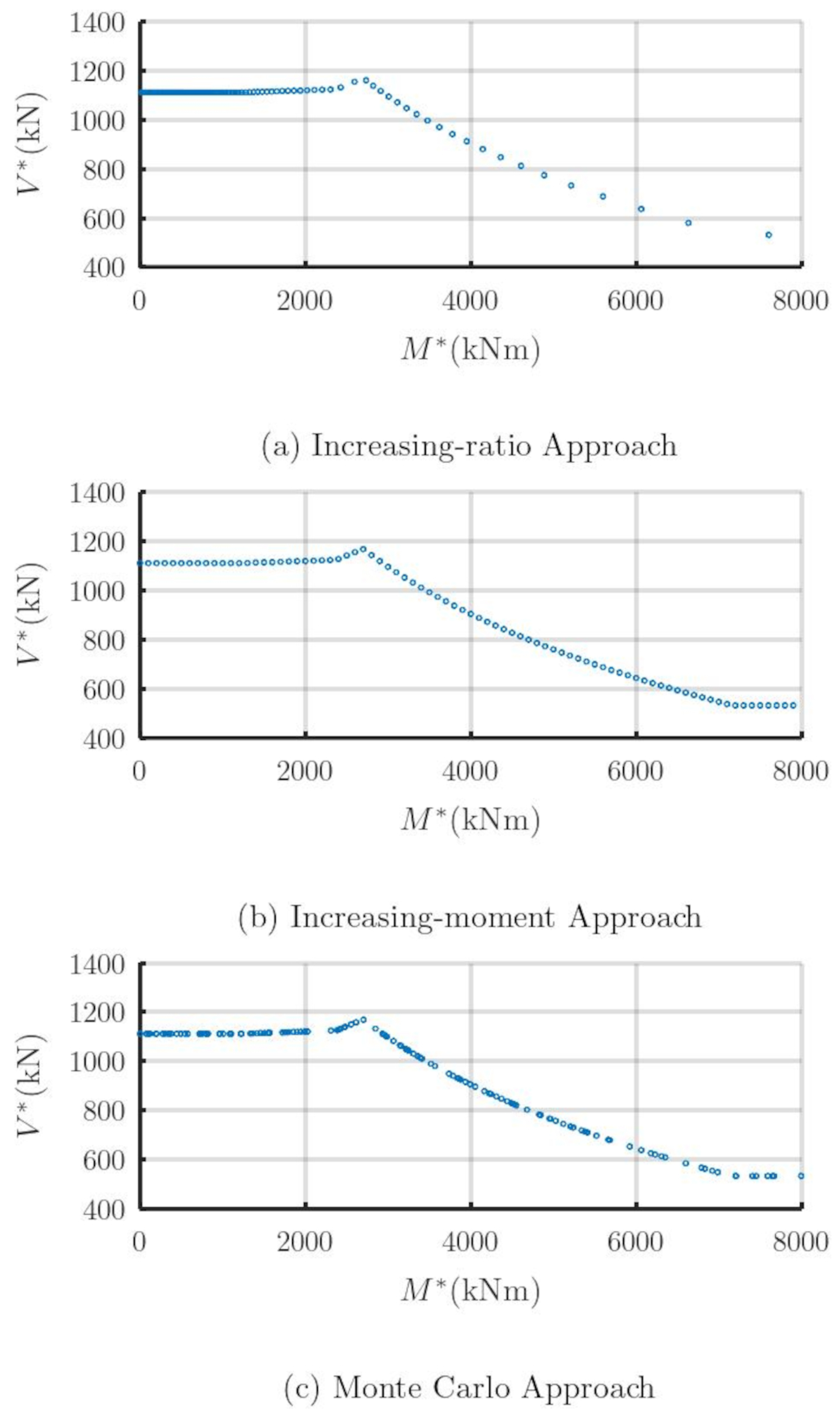
Figure 7.
Flow diagram of the Monte Carlo Simulation Approach.
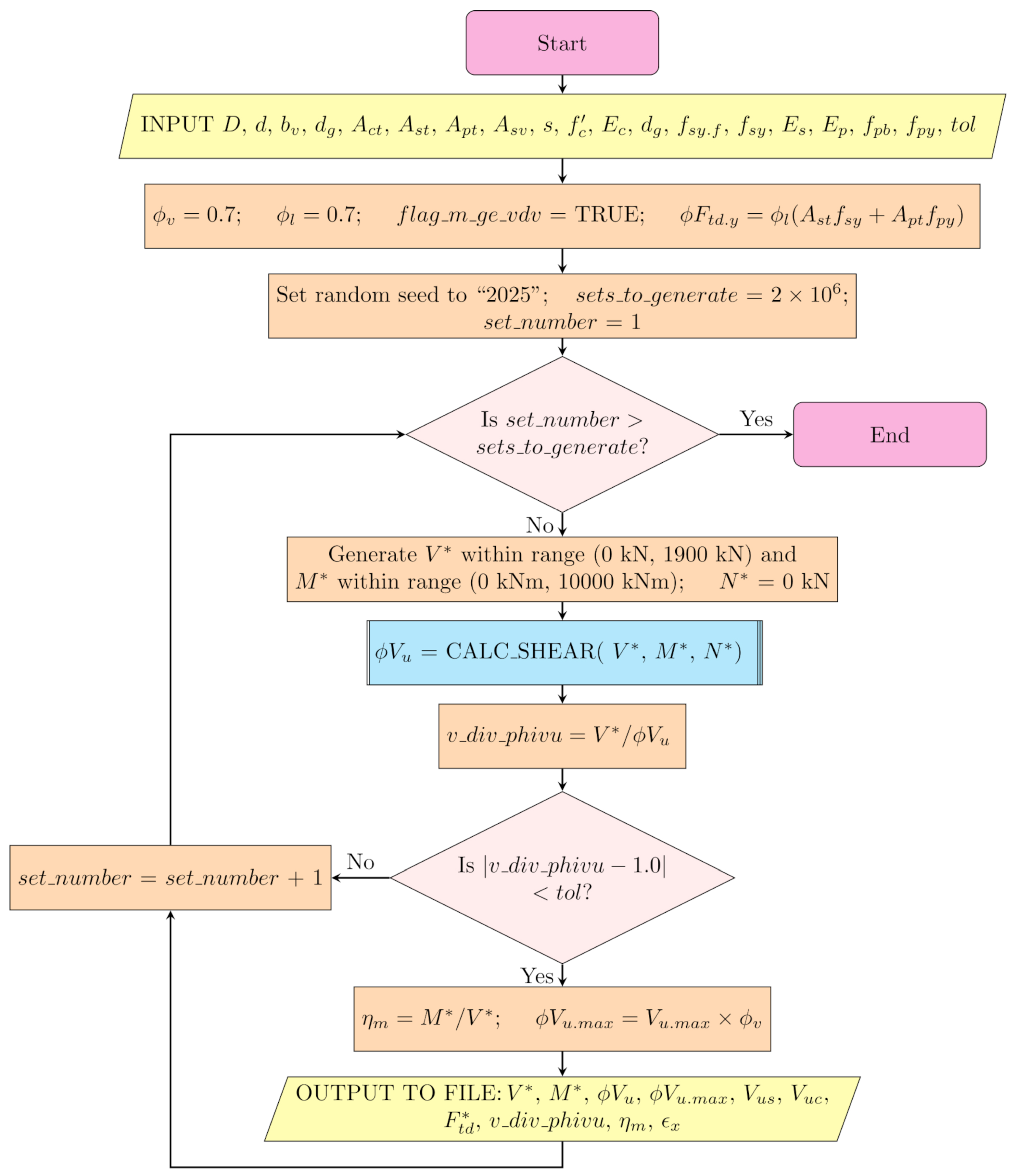
Figure 8.
Design interaction diagram from increasing moment approach for the localized region.
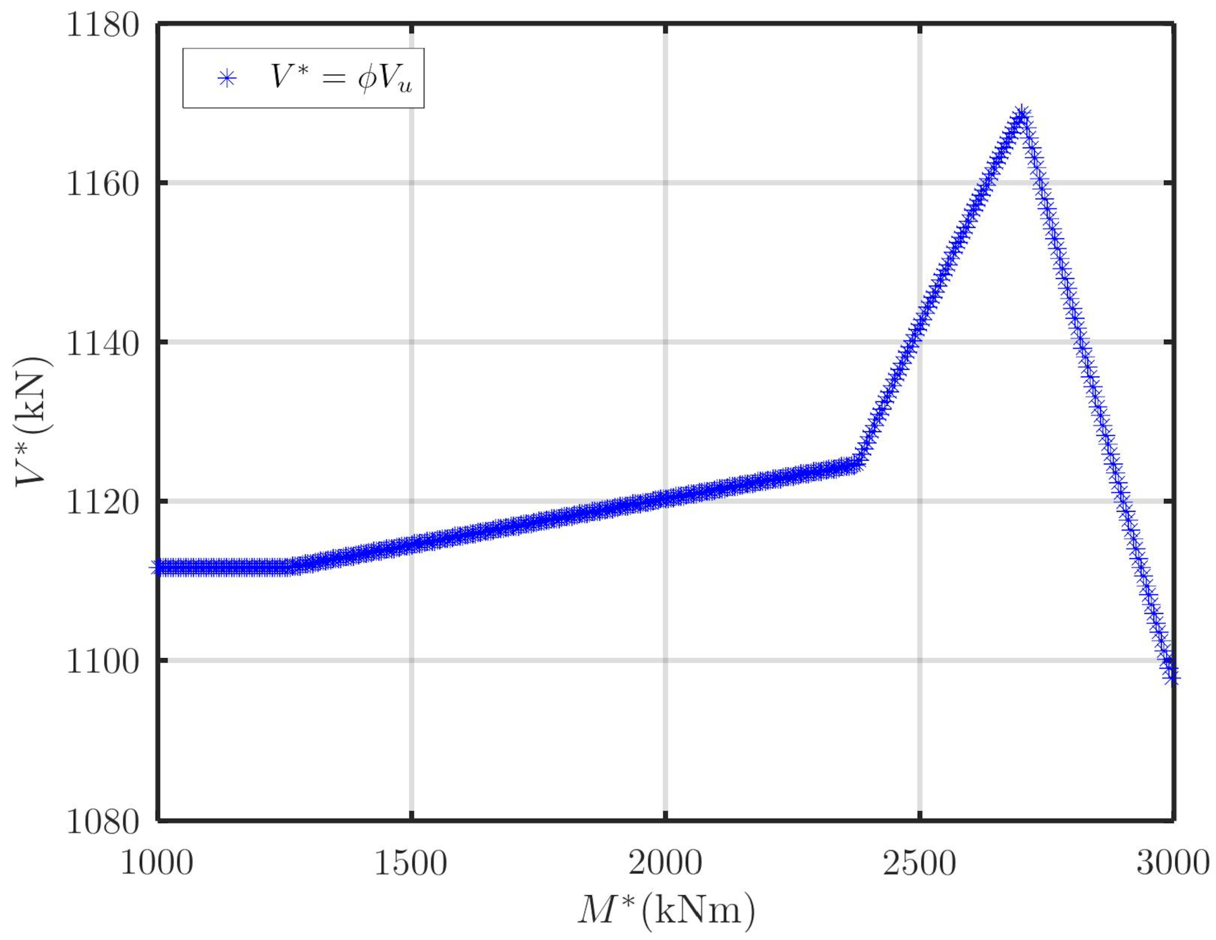
Figure 9.
3-D interaction surface for for strength without the requirement of .
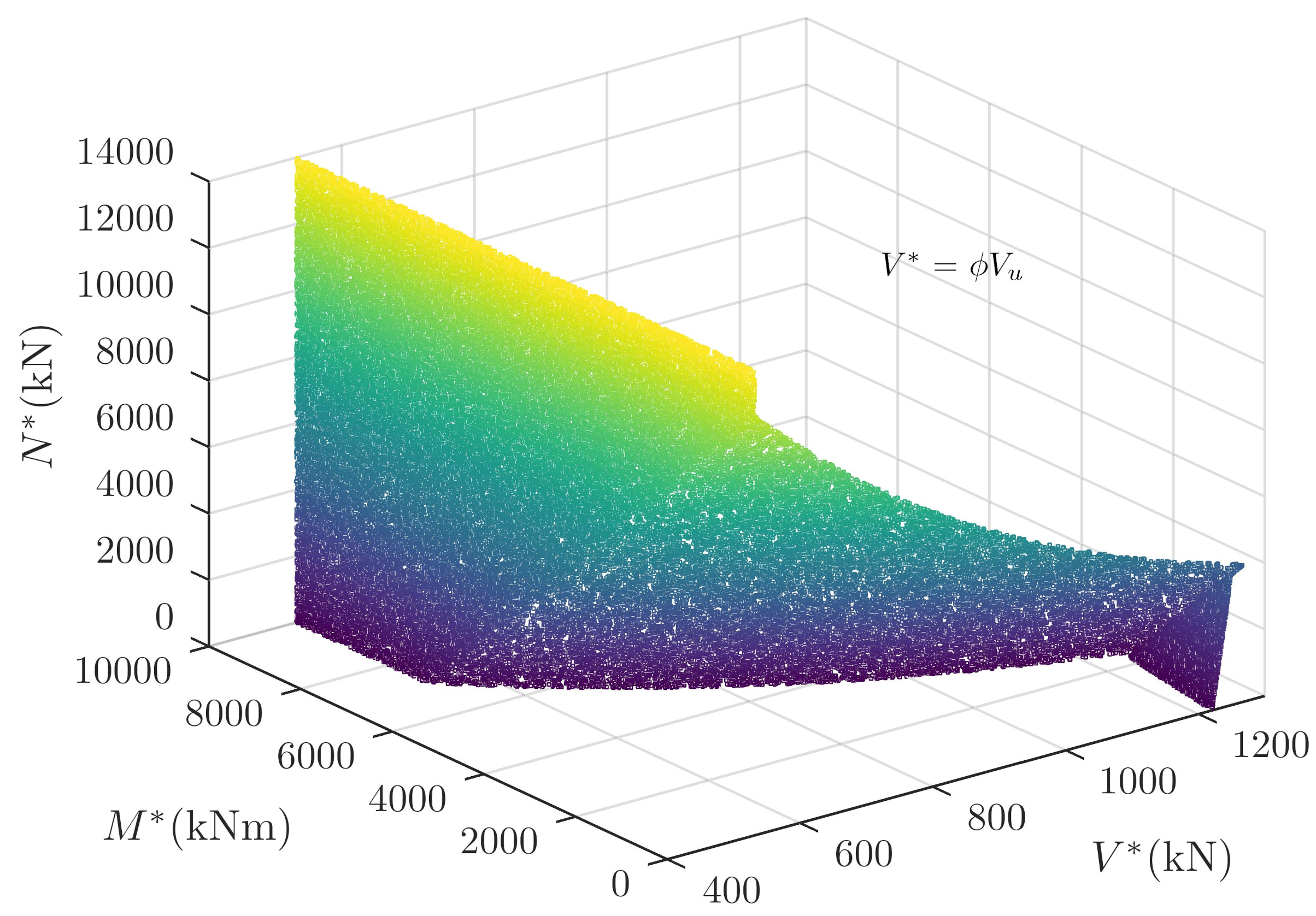
Figure 10.
3-D interaction surface for for strength with the requirement of .
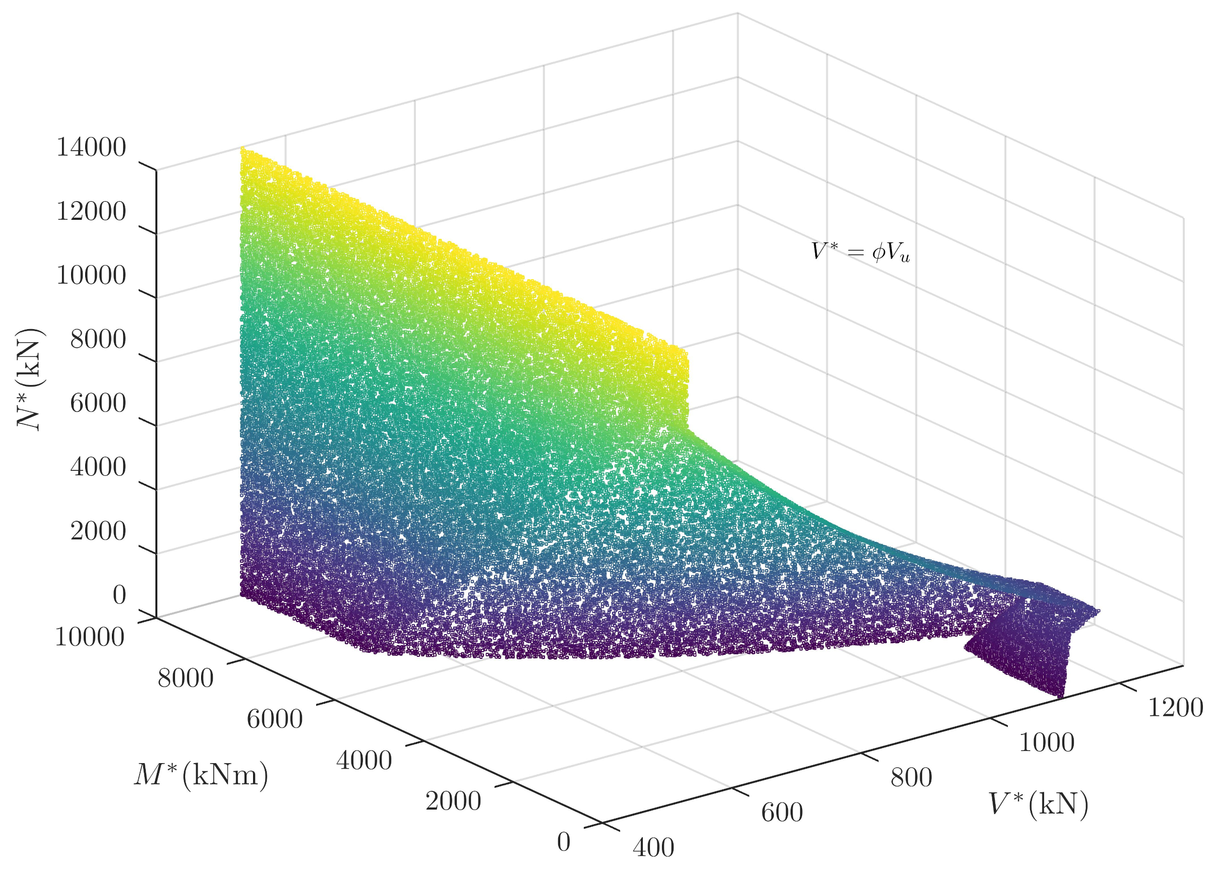
Figure 11.
Scatter plot using points from Monte Carlo approach showing contour curves of interaction of and for = 0.
Figure 11.
Scatter plot using points from Monte Carlo approach showing contour curves of interaction of and for = 0.
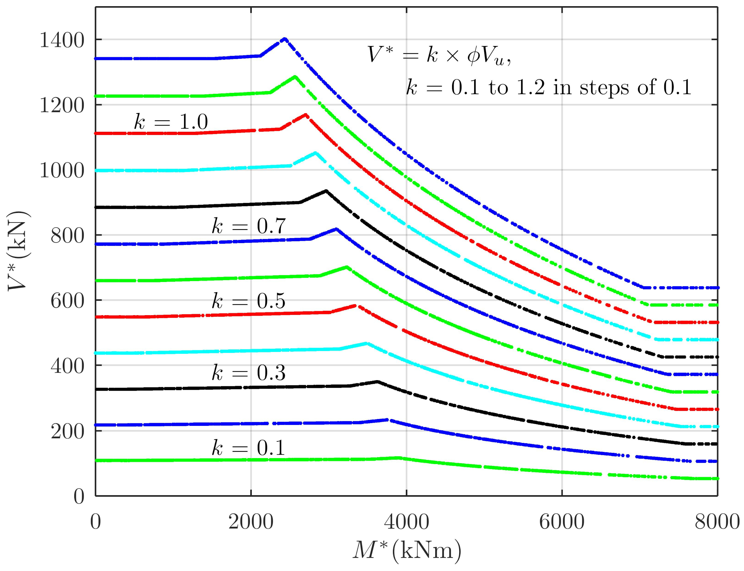
Figure 12.
Scatter plot using points from Monte Carlo approach showing contour curves when limiting the force in longitudinal steel.
Figure 12.
Scatter plot using points from Monte Carlo approach showing contour curves when limiting the force in longitudinal steel.
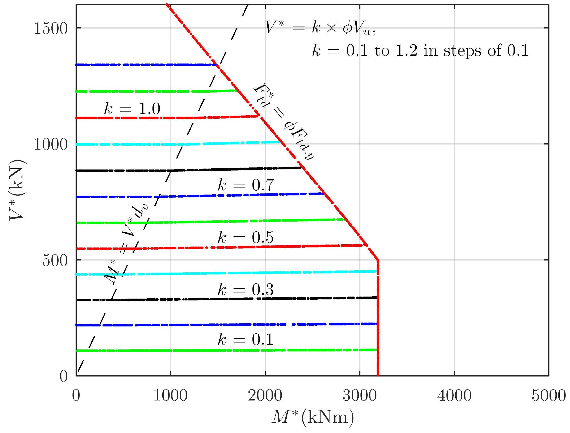
Figure 13.
3-D Scatter plot using points from Monte Carlo approach showing contour surfaces of interaction of , and for .
Figure 13.
3-D Scatter plot using points from Monte Carlo approach showing contour surfaces of interaction of , and for .
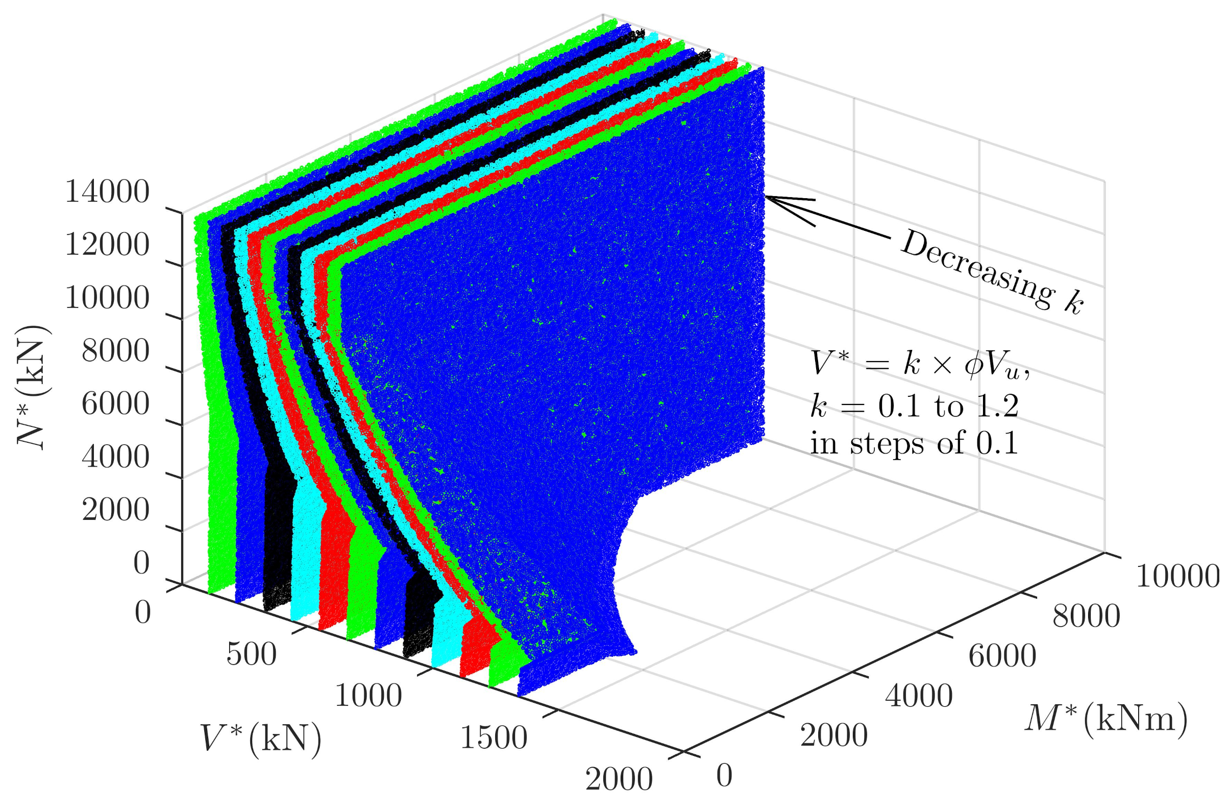
Figure 14.
Interaction curves for various .
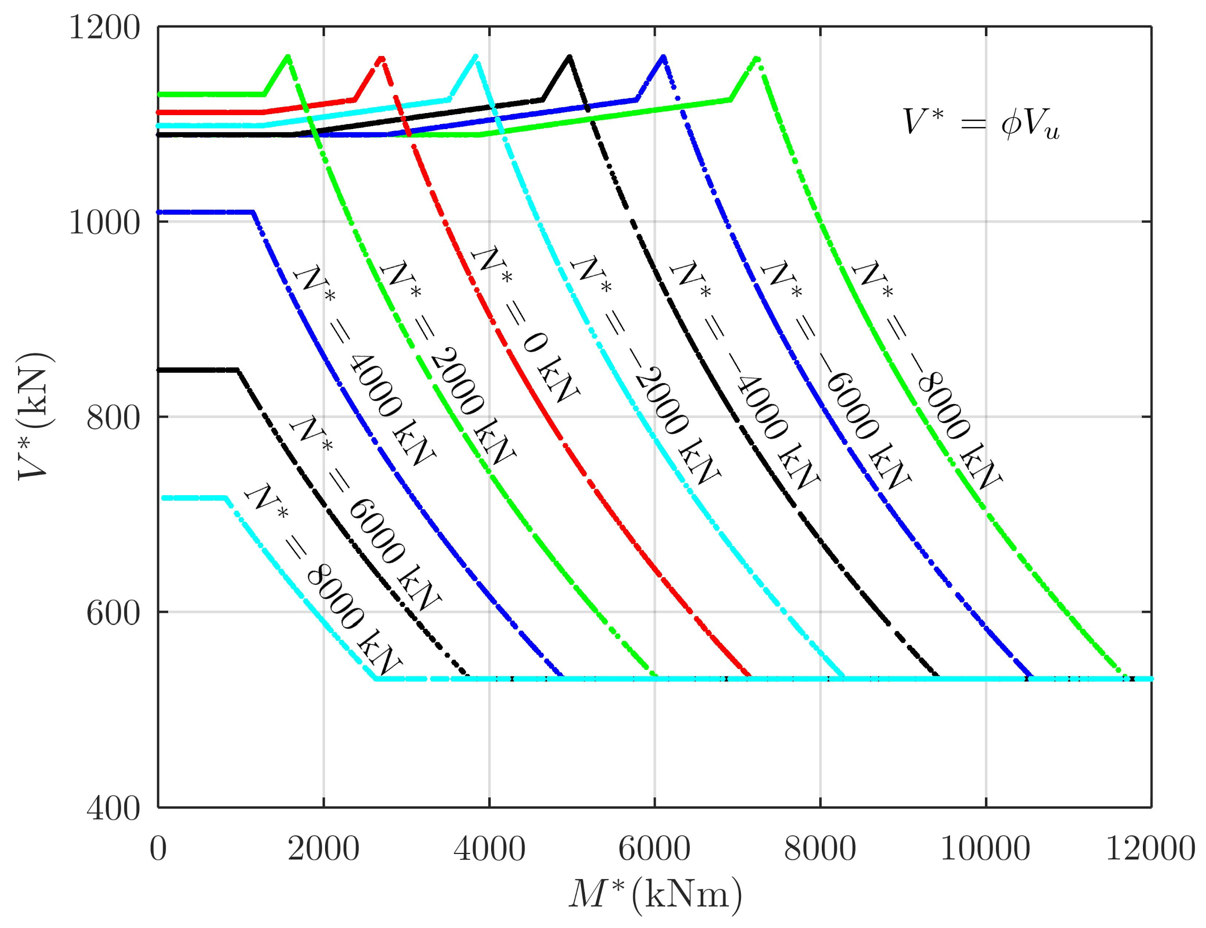
Figure 15.
Interaction curves for various with strength limited by yielding of longitudinal reinforcement.
Figure 15.
Interaction curves for various with strength limited by yielding of longitudinal reinforcement.
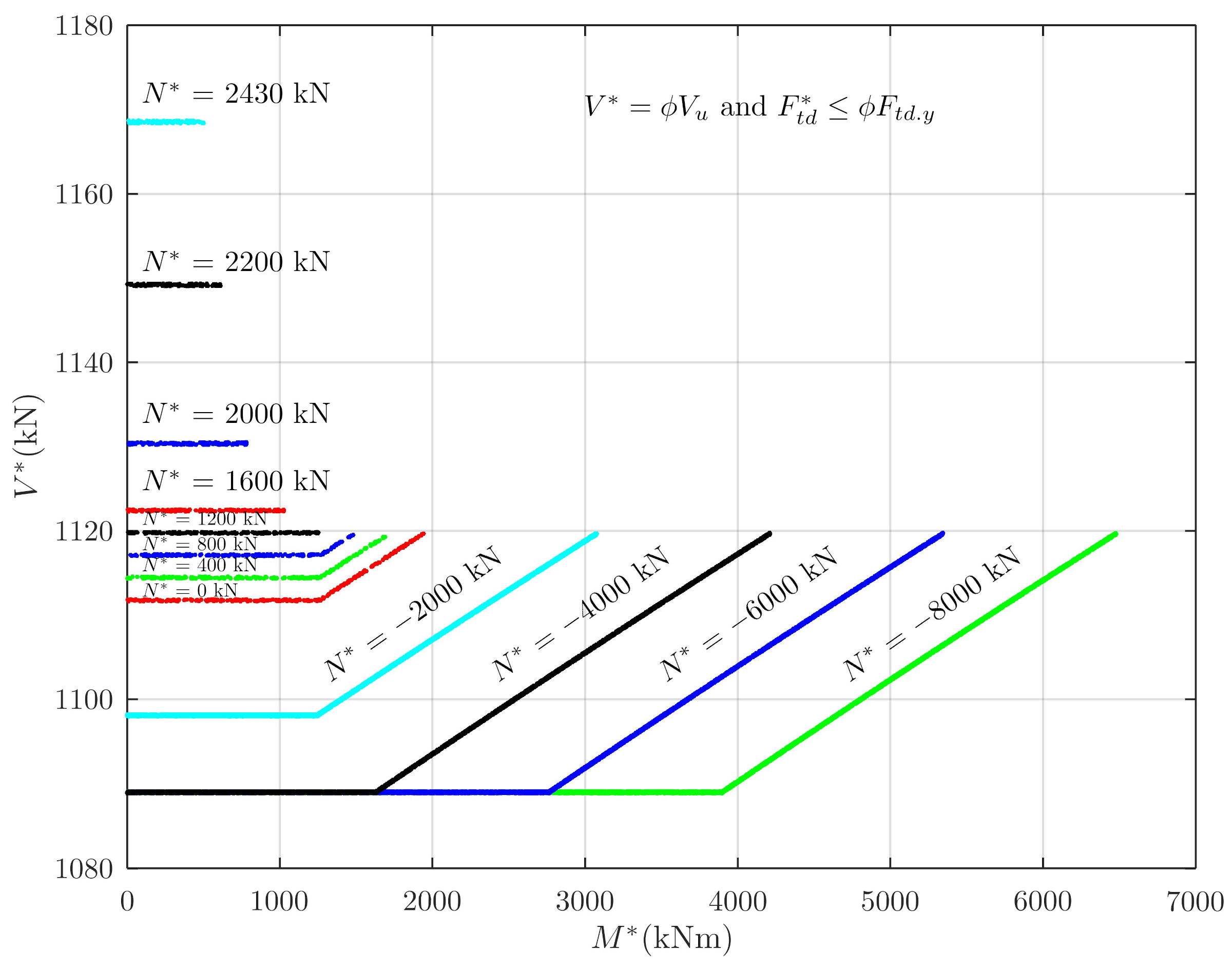
Figure 16.
Plot of versus for both shear and force optimal adequacies for three load effects.
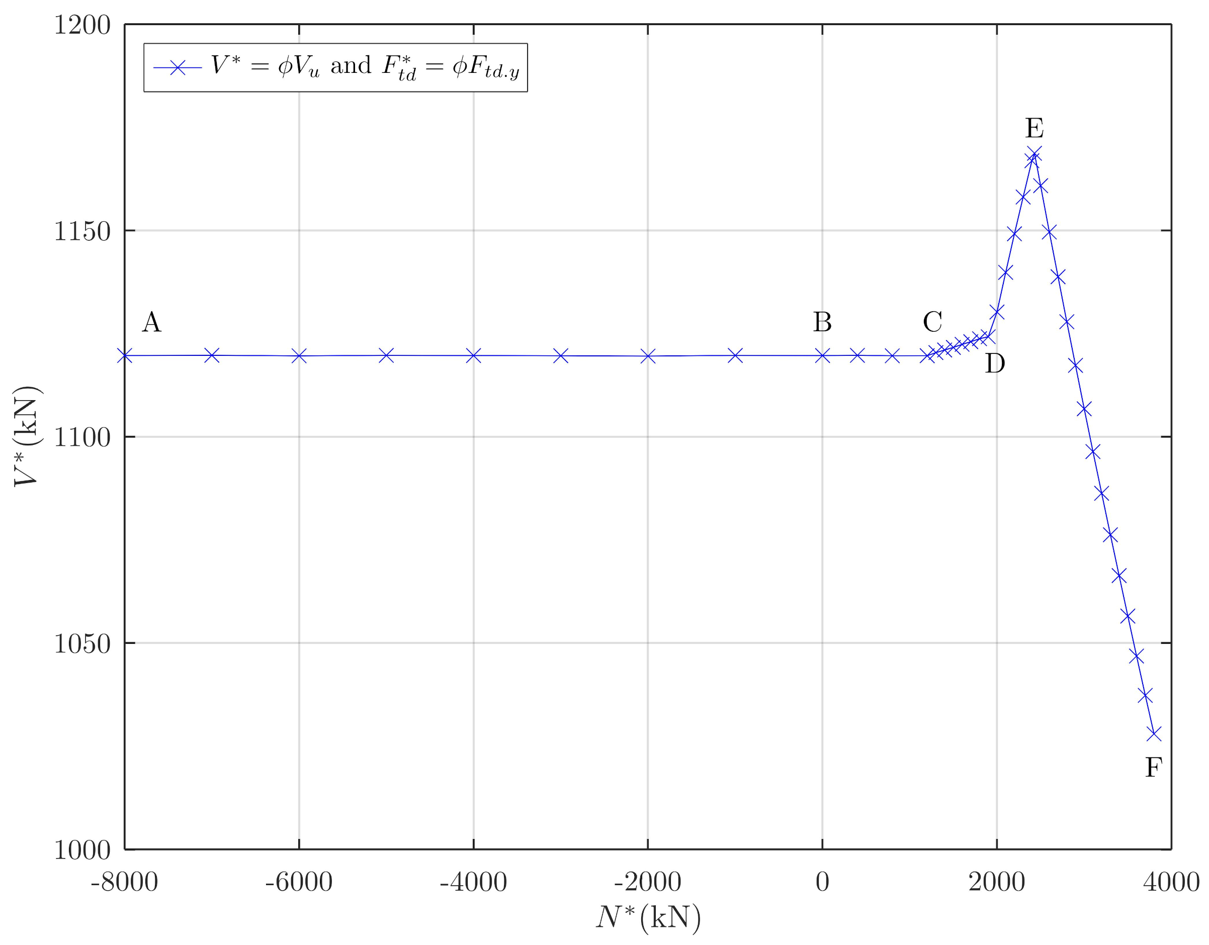
Figure 17.
3-D Scatter diagram from the Monte Carlo approach showing contour curves of interaction of and , kN, for the support section.
Figure 17.
3-D Scatter diagram from the Monte Carlo approach showing contour curves of interaction of and , kN, for the support section.
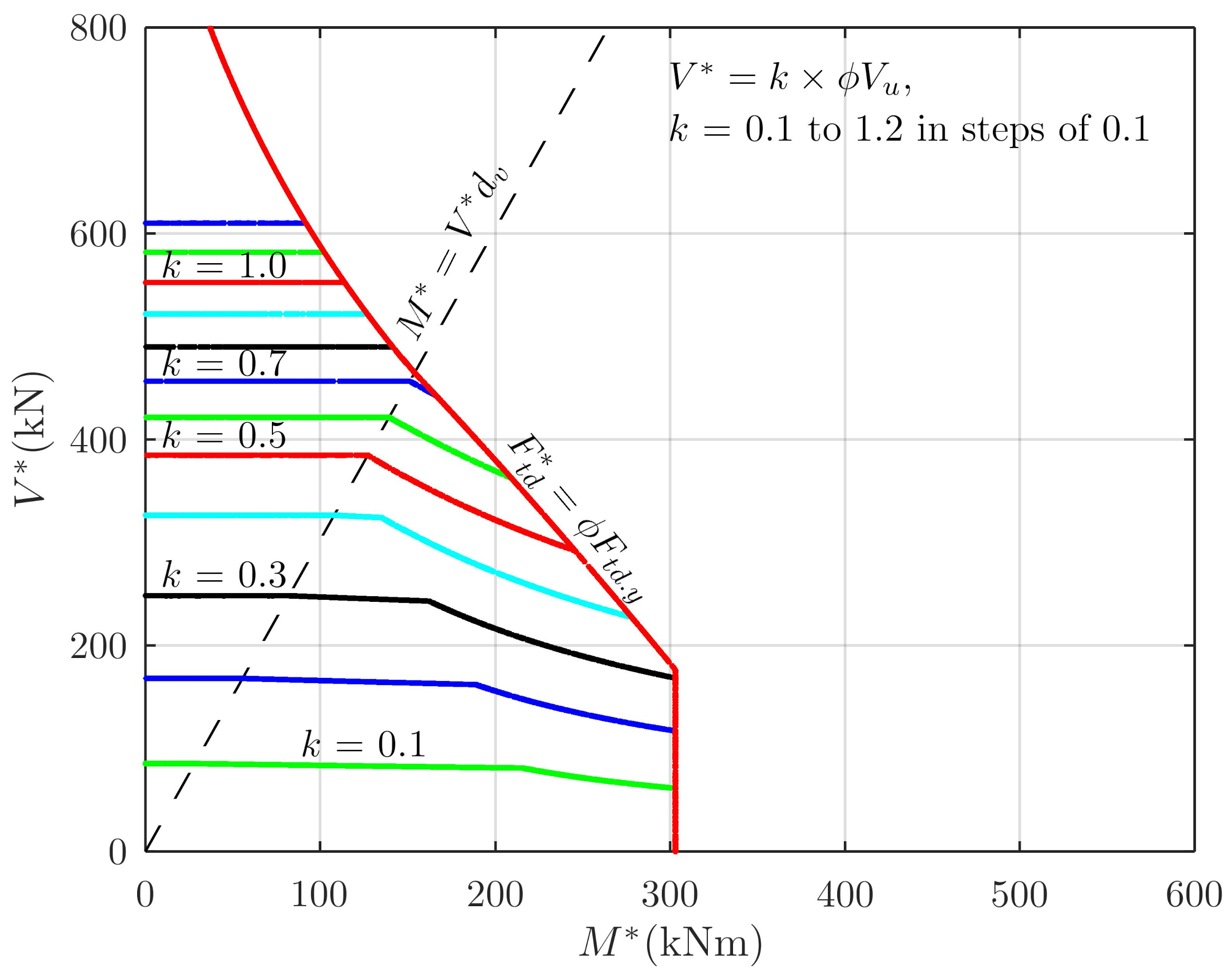
Figure 18.
3-D Scatter diagram from the Monte Carlo approach showing contour curves of interaction of and , kN, for the span section.
Figure 18.
3-D Scatter diagram from the Monte Carlo approach showing contour curves of interaction of and , kN, for the span section.
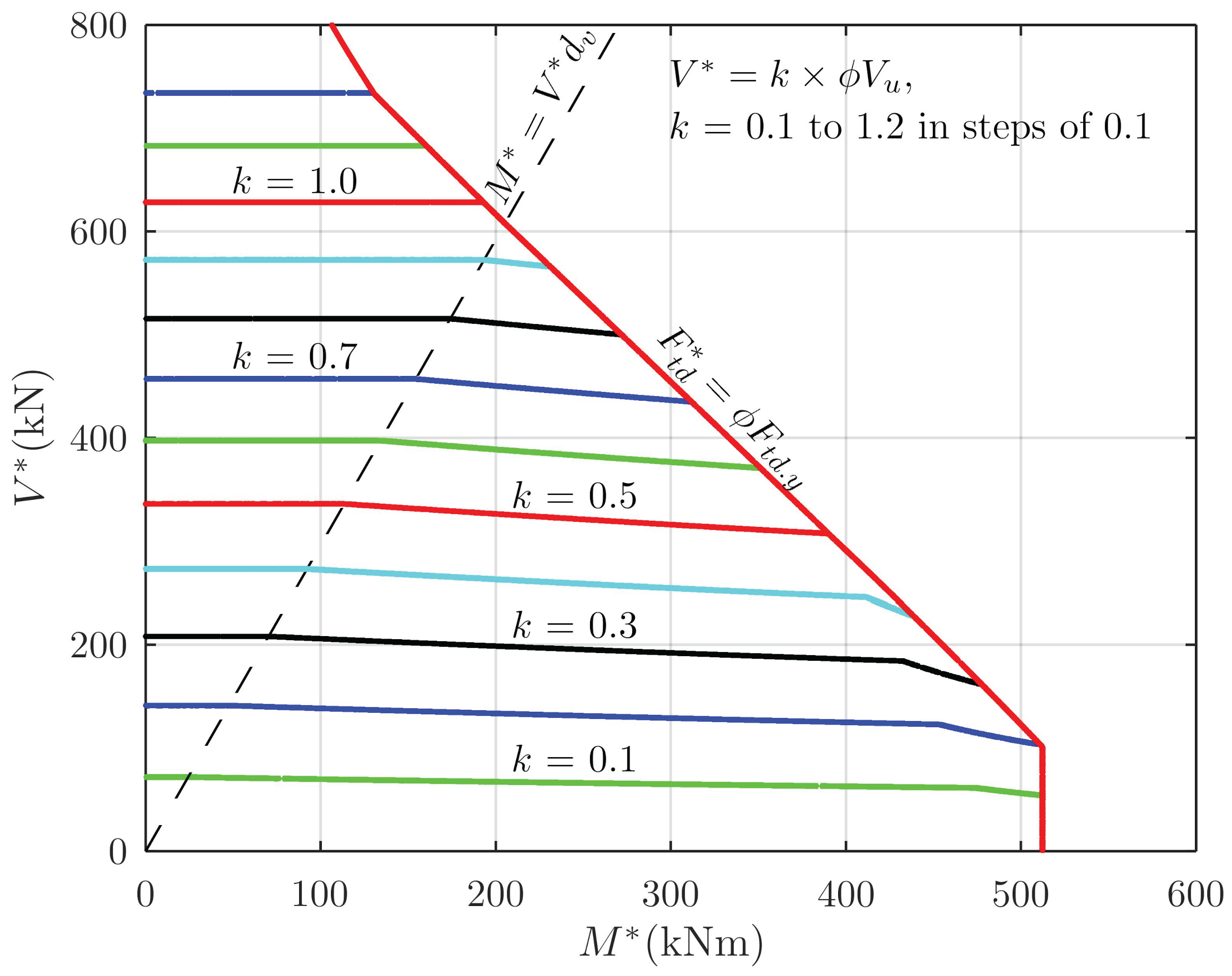
Table 1.
, and from CALC_SHEAR.
| 1 | |||||
| (kN) | (kN) | (kNm) | (kN) | () | (kN) |
| 1767.00 2 | 1362.00 | 1130.46 | 1767.49 | -63.92 | 2138.16 |
| 1717.00 3 | 1717.00 | 1425.11 | 1780.13 | -18.29 | 3044.48 |
| 1782.43 | 1479.42 | 1782.43 4 | -9.88 | 3209.62 | |
| 2170.06 | 1801.15 | 1558.72 | 444.60 | 4022.38 5 |
1 Source of data [14]; 2 non-iterative; 3 iterative; 4 ; 5.
Table 2.
, and from CALC_SHEAR.
| Load Effect | = | ||||
| (kN) | (kNm) | (kN) | () | (kN) | |
| shear | 1362.00 | 1130.46 | 1128.06 | −36.82 | 2541.94 |
| shear | 1111.75 1 | 922.75 | 1111.75 | −73.97 | 1904.01 |
| force | 1470.59 | 1220.59 | 1121.06 | −20.70 | 2815.65 2 |
1. 2
Table 3.
Results for key points of Figure 16.
Table 3.
Results for key points of Figure 16.
| Point | Point | |||||
| Label | Number | (kN) | (kNm) | (kN) | () | |
| A | 1 | 1120 | 6479 | −8000 | −28.8 | 5.07 |
| B | 9 | 1120 | 1942 | 0 | −28.8 | 1.52 |
| – | 11 | 1120 | 1489 | 800 | −28.8 | 1.16 |
| C | 12 | 1120 | 1262 | 1200 | −28.3 | 0.99 |
| D | 19 | 1124 | 857 | 1900 | −1.6 | 0.67 |
| – | 20 | 1130 | 791 | 2000 | 33.3 | 0.61 |
| E | 25 | 1169 | 495 | 2430 | 274.5 | 0.37 |
| F | 39 | 1028 | 5 | 3800 | 607.9 | 0.00 |
Disclaimer/Publisher’s Note: The statements, opinions and data contained in all publications are solely those of the individual author(s) and contributor(s) and not of MDPI and/or the editor(s). MDPI and/or the editor(s) disclaim responsibility for any injury to people or property resulting from any ideas, methods, instructions or products referred to in the content. |
© 2025 by the authors. Licensee MDPI, Basel, Switzerland. This article is an open access article distributed under the terms and conditions of the Creative Commons Attribution (CC BY) license (http://creativecommons.org/licenses/by/4.0/).
Copyright: This open access article is published under a Creative Commons CC BY 4.0 license, which permit the free download, distribution, and reuse, provided that the author and preprint are cited in any reuse.