

Submitted:
10 July 2026
Posted:
13 July 2026
You are already at the latest version
Abstract
We give the operator core of Schrödinger and Dirac dynamics on a framed prime shell \(p=4\kappa+1\), whose capacity \(\kappa\) counts its quarter-turn packets: the shell's information budget. The Lorentzian form depends only on the square class of its temporal coefficient; we prove the drive multiplier canonical and identify this class with the chronon-parity grading. Over the quadratic extension, finite Hamiltonians are self-adjoint and their Cayley steps exactly unitary; the Cayley map identifies the self-adjoint projective line with the norm-one torus, also the boost group transporting the finite Dirac operator (the boost content is deliberately 1+1). The Dirac operator factors exactly into a spinorial Klein-Gordon operator, and a spinor twist forced by the arithmetic makes its evolution unitary, with massless periods a power of \(p\) and mass phases on the same torus. Free evolution is the drive itself; wave transports are isentropic, orbit periods are classified by the shell's two tori, and power maps lose distinguishability by an exact Hartley count. The two wave equations emerge as the two Fourier pairs of one finite shell. The identities are proved in finite-field arithmetic, every quoted example is reproduced by exact scripts, and the continuum enters only as a labelled degenerate idealisation.
Keywords:
finite fields
; finite Dirac operator
; Cayley transform
; Clifford algebra
; Frobenius involution
; Lorentzian quadratic form
; finite-field dynamics
; reversible maps
; information capacity
; Hartley entropy
; finite ring cosmology
1. Introduction
Finite-field models provide a controlled setting in which kinematics, wave evolution, and covariance can be studied without completions, limits, or infinite-dimensional state spaces. They also expose a useful separation that is often hidden in continuum notation: coordinates may live in one finite field, while coefficients for amplitudes, conjugation, and spinorial operators may require a finite extension. The present paper develops this separation for a prime field
its quadratic extension
where is a nonsquare, and the Frobenius involution on K.
The guiding claim is structural. Once the shell, its frame, the quadratic extension, and the Frobenius involution are fixed, the relevant wave identities are finite algebraic identities. Hermitian preservation, Cayley stepping, Clifford factorization, and boost transport are expressed below as equalities of finite matrices and finite maps. All spaces, sums, operators, and transports used in the construction are finite.
This finite level removes several continuum technical burdens from the construction. There are no unbounded operator domains, no convergence questions for infinite sums, no ultraviolet regularization choices, and no measure-theoretic path integrals. What remains is the algebraic operator layer: nondegenerate Frobenius-Hermitian pairings, adjoints, form-preserving propagators, Clifford anticommutation, Dirac-to-Klein-Gordon factorization, and exact transport. The probability calculus and measurement theory of the programme are developed in its companion quantum paper, where the Born rule is obtained as the registration count of shared-core comparison; the present paper supplies the operator identities that construction rides on, and does not re-derive its statistical layer.
The algebraic ingredients used below have standard sources. Finite fields and their quadratic extensions supply the base arithmetic [1]. Quadratic forms over finite fields, their square-class invariants, and the associated finite orthogonal and unitary groups are classical parts of finite geometry and the theory of classical groups [2,3]. Clifford algebras and spinorial representations are algebraic constructions attached to quadratic forms, with treatments that place the gamma-matrix formalism inside the broader theory of Clifford modules and classical groups [4,5]. Cayley-type rational transforms, including the Crank–Nicolson form of time stepping, are a standard route from self-adjoint finite-difference operators to form-preserving discrete updates [6].
Finite quantum models form a second comparison layer. Schwinger’s unitary operator bases and the finite phase-space constructions of Wootters and of Gibbons, Hoffman, and Wootters show how finite algebra can carry quantum kinematics [7,8,9].
Galois-field and modal quantum theories study state spaces, observables, spin models, and the finite-field status of probability and spectra [10,11,12,13]. Lattice and automaton approaches to relativistic wave equations show how Weyl and Dirac dynamics can arise from exact local unitary update rules on discrete carriers [14,15,16,17,18].
Another closely related finite-quantum perspective was proposed by Carroll [19], who showed that standard finite-dimensional unitary quantum mechanics admits a completely discretized reading when the Hamiltonian spectrum is commensurable: the phase evolution closes on a finite torus, allowing continuous time to be replaced by a finite cyclic sequence of states. The present construction is aligned with that finite and reversible viewpoint, but implements it inside a finite algebra itself. The coefficient field, Hermitian form, Cayley propagator, Lorentzian extension, Dirac operator, and information counts are all finite algebraic objects from the outset, rather than discretizations of a surrounding complex Hilbert-space continuum.
The present construction uses this prior algebraic and finite-quantum terrain inside the finite ring cosmology (FRC) shell setting [20]. In the FRC framework, a symmetry-complete prime shell is a framed finite field with , the capacity: the additive shell, the multiplicative phase cycle of the drive , and the derived quarter-turn with coexist in the same finite arithmetic domain. The broad physical interpretation of these shells belongs to the FRC references; the present paper uses the finite algebraic data, and states its shell readings as tagged identifications. Symmetry-complete shells carry an internal Euclidean phase datum and a framed shell geometry [21], while the Euclidean-Lorentzian split is tied to the square class of a nonsquare coefficient and its quadratic extension [22]. The nonsquare coefficient supplies the coordinate quadratic form
on . The square root w of is not an element of ; it belongs to the quadratic extension K. Two exact refinements of this split are proved in Section 2: the coefficient matters only through its square class, whose canonical representative is the drive multiplier itself, ; and the square class is the chronon-parity grading of the shell, which separates the one-way temporal coefficient from the two-way constant of the FRC constants web. In the present paper, the extension K is used as a coefficient field for Hermitian forms, Cayley dynamics, gamma matrices, and spinor amplitudes. The construction has two operator layers.
First, for a finite Euclidean configuration space , the function space carries a Hermitian form
Translations are unitary, the finite Laplacian associated with a chosen ordered frame is self-adjoint, and finite Hamiltonians of the form
are self-adjoint. For each trace-zero parameter with , the Cayley operator
is defined whenever is invertible. It preserves the Hermitian form exactly, and the scalar Cayley map is shown to be a bijection from the Frobenius-fixed projective line onto the norm-one torus of K: the finite Cayley transform, from self-adjoint data to the unitary torus.
Second, the coordinate shell
with the form (1) supports a finite Dirac-type difference operator with K-valued spinors. The gamma matrices are explicit matrices over K and satisfy
The corresponding Dirac operator factors exactly through a spinorial Klein-Gordon operator. A finite boost subgroup acts by exact transported Dirac operators, with an explicit spin lift; the subgroup is identified exactly as the norm-one (non-split) torus of the extension.
The construction below keeps the coordinate/coefficient distinction explicit throughout. Its scope is the algebraic operator layer: Frobenius-Hermitian Schrödinger-type propagation, Clifford factorization, and Dirac-type Lorentzian transport inside one finite scheme — together with the shell reading this layer supports: the free Schrödinger evolution is the drive itself, exactly, and the Dirac operator develops the shell along its meridians (Section 7).
The final layer records exact finite counts. For a finite map , the image count and loss factor separate reversible transport from many-to-one compression. Cayley propagators and boost transports are bijections on their finite state spaces, and their orbit periods are classified: kinetic Hamiltonians give unipotent propagators of order exactly , potential Hamiltonians give norm-one phases of order dividing — the translation and boost tori of the shell. Shell power maps on can be many-to-one, with exact loss factor . These counts are used only as finite diagnostics of reversibility; packet transfer, invariant coding, and shell-to-shell fiber profiles are a separate finite-transfer problem, outside this paper’s scope.
The paper is organized as follows. Section 2 fixes the shell, frame, coefficient, and coordinate data, the canonical Lorentzian coefficient, and the parity grading. Section 3 develops Hermitian function spaces and finite difference operators. Section 4 proves exact preservation for Cayley dynamics and the finite Cayley transform. Section 5 constructs the gamma matrices, Dirac operator, boost torus, and factorization. Section 6 records the exact reversibility counts and orbit periods. Section 7 states the shell reading: zonal and meridional dynamics. Section 8 and Section 9 summarize the scope and the next finite-field problems.
2. Shell, Frame, Coefficient, and Coordinate Data
Let
be prime, with the shell’s capacity. Then is cyclic of order . The capacity is an information count: the states of the phase cycle fall into exactly four-element quarter-turn packets (the cosets), two bits per packet in the labelled logarithmic reading, so measures the shell’s distinguishability budget. The shell is read through a relative frame
following the FRC frame convention [20,21]: the origin 0 and unit 1 are pure position and scale, the affine gauge of the shell; g is the multiplier of the frame-holder’s own drive , invariant under every reframing (conjugating the drive by returns a drive with the same multiplier), with ; and the chronon t is the observer’s present tick, the frame’s one free temporal datum. From these data the shell derives its oriented quarter-turn
The orientation is derived, not chosen: a winding mode is read through the fixed frame by pullback, so it registers phase opposite to its winding per chronon, and the oriented quarter-turn is the phase the minimal material mode accumulates over one quarter-period of forward drive. This is the finite Euclidean phase datum used below; Figure 1 shows the smallest such shell in its two canonical presentations.
Remark 1
(Role of the congruence condition). The condition is the shell condition that places the Euclidean phase element inside the base field . For abstract Clifford algebra alone, one can often move the required square roots into a coefficient extension. What is lost when is not the possibility of writing related matrices, but the FRC separation used here: the Euclidean phase is no longer internal to the base shell. The present paper works in the symmetry-complete regime where the Euclidean phase lives in and the Lorentzian nonsquare coefficient is represented by a separate extension K.
Remark 2
(Shells in play). Several finite structures appear in this paper and are named apart throughout: the worked Subject shells and ; the coordinate shell ; and the coefficient field K. Carrier-scale statements of the FRC programme are transfer targets of the shell-generic identities proved here, never sites of computation in this paper. Every congruence below names its modulus.
The elementary arithmetic maps on the shell are
where , , and . The maps and are bijections. The power map on is bijective if and only if .
Fix a nonsquare and define
Since is a nonsquare, is irreducible over , so . Every element of K is written uniquely as
The Frobenius involution is
It satisfies
The fixed field of this involution is . The trace-zero part is
Remark 3
(Two conjugation registers). The derived quarter-turn isfixedby Frobenius: for the Hermitian structure of this paper, is a real quantity, and the anti-fixed element is w. The two imaginary units serve different registers — the internal Euclidean phase of the shell, w the conjugation of the coefficient extension — and neither substitutes for the other. This register separation is used throughout.
The element w is used only on the coefficient side. The coordinate quadratic form below has coefficients in because .
The choice of resolves at two levels, both exact.
Lemma 1
(The class is the datum). has order two, so the nonsquares of form a single class: for any two nonsquares there is with , and the rescaling identifies the corresponding quadratic forms. All constructions below therefore depend on ν only through the nonsquare class; the choice of representative carries no geometric content.
Lemma 2
(The drive is canonical among the frame’s named residues). Callnamed residuesof the frame the tuple entries and the derived data , , , together with the constant seats 2, , of the programme’s residue web. The drive multiplier is always a nonsquare: for primitive g. Among the named residues it is the only element whose class is nonsquare on every symmetry-complete shell: 2, , and are squares exactly when κ is even (); is a square iff κ is even (an eighth root of unity exists iff ); and and have no stable class. By Lemma 1 the choice carries no geometric content; canonicity is naming, relative to this inventory, and within it the selection is unique. The canonical Lorentzian coefficient is therefore
stable under the reframing gauge (), so that adjoins the half-step of the drive, .
Proof.
Primitivity gives the first claim. The parity criteria for 2 and are the second supplementary law together with ; the criterion for is the cyclicity of ; the instability of e and is witnessed already by against (Section 5, examples). All claims are additionally machine-verified in exact arithmetic on every symmetry-complete shell (Section 1). □
The general theorems below are stated for arbitrary nonsquare , per Lemma 1; the worked examples instantiate the canonical .
Remark 4
( is not ). In the FRC constants web the speed of light is the base residue with , which by Lemma 2 is asquareprecisely on the admissibility class κ even — on those shells c is base-rational while is not. The continuum habit of reading the temporal coefficient as is therefore unavailable here; the exact relation between the two seats is Corollary 1 below.
The square-class structure just used has a dynamical form.
Theorem 1
(The square class is chronon parity). For a primitive drive g, the squares of are exactly : the quadratic class of a residue is the parity of its drive-step count . In particular the signature (nonsquare) class is the odd-parity class, with canonical representative the single chronon step g.
Proof.
is the index-two subgroup of the cyclic , and it consists of squares; conversely every square lies in it. □
Theorem 2
(Norm growth and parity). One chronon of drive multiplies every Frobenius norm by : for all , and is a square (even parity), while the single-chronon multiplier g is odd-parity and the equation has no solution in for nonsquare ν.
Proof.
since is Frobenius-fixed; . Insolubility of is the definition of a nonsquare. □
Remark 5
(One-way and two-way transport, tagged). In the FRC reading, comparison-type (two-way) readings are even-parity by Theorem 2, the one-way single-chronon multiplier is odd-parity, and the null-cone slope is not a base-field ratio: light-like transport carries no registered velocity, only its square class — the causal character of the interval.
Corollary 1
(The two speed-of-light seats). Since , the temporal coefficient factors identically on every shell:
and the cofactor carries the entire signature bit in both parities: is odd iff κ is even, is odd always. The registered two-way constant (even-parity exactly on the admissibility class κ even) and the odd-parity one-way coefficient ν are the two exact factors of the continuum’s single symbol: the identification “” is the collapse of the parity grading in the continuum chart, where every positive scalar is a square. The reframing flip preserves the parity class while reversing the one-way direction: the one-way speed is gauge — the finite form of the synchronization freedom — while the two-way constant is invariant.
The Lorentzian coordinate shell is
It is equipped with the diagonal quadratic form
Let
and write for the entries of this fixed diagonal matrix. The subscript notation denotes matrix entries only; no index-raising convention is used. The time coordinate is read in the chronon-count chart: one unit step of is one chronon of drive, so the additive translations of realise the translation cycle while the drive’s own phase runs on (Section 7).
The finite orthogonal group of the coordinate form is
The explicit finite boost subgroup used in Section 5 lies in this group and is identified there with the norm-one torus of K.
Remark 6
(Coordinate and coefficient roles). The coordinate shell is . The coefficient field for amplitudes, Hermitian conjugation, gamma matrices, and spin lifts is K. This separation is useful because the Lorentzian coefficient ν is already present in , while its square root w is available only in K. Earlier FRC terminology often describes the Lorentzian stage as the quadratic extension ; the present construction is the -coordinate operator layer inside that framework, not a replacement for it [22].
3. Finite Hermitian Function Spaces
Let X be a finite set. Define
the K-vector space of all K-valued functions on X.
Definition 1
(Hermitian form). For , set
Lemma 3.
The form (10) is Hermitian and nondegenerate.
Proof.
Hermitian symmetry follows from
For nondegeneracy, let . Choose with and define , for . Then
□
Since K has no compatible order, the word Hermitian here denotes the algebraic preservation of the involutive form (10). It is not a positivity statement.
Remark 7
(Algebraic scope of Hermitian language). In this paper the Hermitian form supplies three pieces of finite linear algebra: a nondegenerate pairing, an adjoint operation, and the form-preservation condition . Self-adjointness means with respect to this pairing, and it is used to prove exact Cayley preservation in Section 4. Probabilistic interpretation, ordered expectation values, and spectral observables require additional finite-field quantum structure beyond this pairing.
Definition 2
(Adjoint). Let be K-linear. The adjoint is the unique K-linear operator satisfying
for all .
The adjoint exists and is unique because (10) is nondegenerate and is finite-dimensional over K.
For , let
with its additive group law. For , define
Proposition 1.
For every , the translation operator is unitary on and
Proof.
The map is a bijection of . Reindexing gives
Similarly,
□
Let be an ordered basis of . Define
Proposition 2.
The finite Laplacian is self-adjoint on .
Proof.
For each , and . Thus each summand in (14) is self-adjoint. □
Let . Multiplication by V defines
Since is fixed by Frobenius, is self-adjoint.
Definition 3
(Finite Hamiltonian). For , define
Corollary 2.
The Hamiltonian is self-adjoint.
Proof.
Both and are self-adjoint, and is fixed by Frobenius. □
Remark 8
(The stiffness normalisation). The coefficient ϰ is the stiffness of the kinetic term, with the unit-capacity normalisation used in the examples. Two visually similar symbols are in play and never interchange: the capacity κ (the shell parameter, ) and the stiffness ϰ (the kinetic coefficient); the distinction is the corpus-wide FRC convention, and ϰ appears only in and the examples.
Definition 4
(Finite unitary group). For a finite set X, write
If , a choice of ordering of X identifies with and (10) with the standard Frobenius-Hermitian form. The group is therefore the finite unitary group attached to the quadratic extension , one of the classical finite groups of Lie type [3].
Lemma 4.
Let , let , and let . Define
Then, for each μ,
Proof.
For translations,
The finite difference identities follow from the definitions. □
4. Cayley Dynamics on Euclidean Shells
Let be a self-adjoint finite Hamiltonian on .
Definition 5
(Cayley step). Let , so . If is invertible on , define
Equivalently,
Definition 6
(Admissible Cayley parameters). For self-adjoint H, set
The set is finite and nonempty because .
Remark 9
(Admissibility). Admissibility is governed by the finite determinant condition
Thus the excluded trace-zero parameters are exactly the roots, inside , of the finite polynomial . The example below records one nonzero admissible parameter; a general classification of depends on the finite Hamiltonian.
The parameter always gives the identity propagator. The substantive admissibility question is therefore the nonzero part of .
Theorem 3
(Exact Hermitian preservation). Let H be self-adjoint and let . Then
for all .
Proof.
Since and ,
The invertibility of implies the invertibility of by taking adjoints. Hence
All factors are rational functions of H, so they commute. Therefore
This gives (19). □
Corollary 3
(Finite periodicity). For every , the Cayley orbit is periodic.
Proof.
The vector space is finite. The group is finite, and by 3 the operator belongs to it. Hence some positive power of is the identity. □
Theorem 4
(The finite Cayley transform). Let be nonzero and let
Then φ is defined for every , takes values in the norm-one torus
and, extended by , is a bijection from the projective line onto . In particular , and the unitary group of the one-dimensional Hermitian space K is exactly .
Proof.
Write , . The denominator has Frobenius norm , which vanishes only if is a square — impossible. The same computation gives since . The map is injective as a nonconstant Möbius map, has points, and (the norm is surjective onto with fibers of equal size), so injectivity gives bijectivity. The group statement is the definition of . □
The Frobenius-fixed line — the self-adjoint data — and the unitary torus are therefore in exact bijection: the finite form of the Cayley transform from self-adjoint operators to unitaries. The same torus reappears in Section 5 as the boost group; evolution phases and boosts share one structure.
Remark 10
(The forward step). The map inverts every : it is the orientation gauge of the evolution torus, the same as the derived orientation of the shell. The forward step is therefore not a free choice but imports the derived orientation (a winding mode registers phase opposite to its winding per chronon); the natural normalisation composes the two quarter-turn seats of the scheme, the internal and the extension’s w:
the finite Crank–Nicolson seat of the evolution kernel at unit stiffness .
Example 1
(The case ). Let with frame , so , , and the canonical coefficient is ; let . Take , , , , and . Then . Since H is nilpotent (8), is invertible forevery: is a general fact for kinetic Hamiltonians, not a observation. The example’s content is the orders: writing ,
Thus every vector in returns after 13 Cayley steps for each non-zero trace-zero parameter in this example; Section 6 derives this order as the unipotent (translation-torus) case of the general period dichotomy. The supplementary scripts (Section 1) reproduce the full admissibility and order computation by exact arithmetic in .
The Cayley construction is an algebraic finite analogue of unitary time stepping. The preserved quantity is the Hermitian form (10); no order or probability measure is used.
5. Dirac-Type Operator and Finite Boost Transport
Let with standard ordered basis and quadratic form from (8). A spinor field on Y is a function
The spinor field space is
For an ordered basis of Y, define directional forward differences
Because Y is an additive group, these finite differences commute for a fixed frame E.
Let
Since , the Pauli identities
hold over K.
Define
and set
Proposition 3
(Clifford relations). The matrices (21) satisfy
Proof.
The Pauli identities give and for . Also . The mixed block product is
so . Since and ,
and all mixed anticommutators vanish. □
5.1. Standard Finite Dirac Operator
Define the scalar finite Klein-Gordon operator on Y by
Its spinorial extension is
Definition 7
(Standard finite Dirac operator). Define
on . For , the finite Dirac equation is
Theorem 5
(Dirac-to-Klein-Gordon factorization). On ,
Proof.
Set
Since , , and ,
Let and assume
Define
Then
Define
Proposition 4
(Spin conjugation). The spin lift satisfies
Proof.
The inverse formula follows from . The identities
give (31) and (32) by direct multiplication. The matrices and commute with , because each anticommutes with both factors and . Hence and . □
Definition 8
(Coordinate boost). For satisfying (27), define
Proposition 5.
The matrix belongs to .
Proof.
A direct calculation from (30) gives
For the displayed block, this identity is exactly . The last two coordinates are fixed. □
Proposition 6
(Boost subgroup). The set
is a subgroup of .
Proof.
Let and in . Their product is
The norm satisfies
Direct multiplication of the matrices (34) gives
Also and . Hence, is a subgroup. □
Lemma 5
(The boost group is the non-split torus). The map is a surjective homomorphism from onto with kernel the scalar line , and the boost entries are the coordinates of :
Hence
cyclic of order : the boost group is the norm-one (non-split) torus of the extension, the same torus that carries the evolution phases of Theorem 4, and it contains an element of order three if and only if .
Proof.
Multiplicativity is the subgroup law just proved. The entries (30) are homogeneous of degree zero in , so the scalar line acts trivially; conversely , forces and , hence . For the Hilbert-90 form, by direct expansion, with ; the identity of Proposition 5 is this norm-one condition. The quotient is cyclic of order and realises it inside , which has the same cardinality. The triality clause is Cauchy’s theorem in a cyclic group. □
5.2. Transported Dirac Operators
Let and set
Define the pullback on spinor fields by
Lemma 6.
For every μ,
Proof.
For and ,
which is . □
For , define the spinor transport
The transported Dirac operator is
Proposition 7
Proof.
Corollary 4
(Transported Clifford relations). For every and spin lift S, the family satisfies
Proof.
Conjugation by S preserves anticommutators. □
For the boosted frame, set
and
Theorem 6
(Transported factorization). For every and spin lift S,
Proof.
Use Proposition 7, the commutativity of the finite differences in the frame , and the transported Clifford relations. The calculation is identical to the proof of 5. □
Corollary 5
(Exact covariance of the transported family). For with spin lift S and every ,
Consequently, a solution of is transported to a solution of
5.3. Symmetric Dirac Operator and Exact Unitary Evolution
The forward differences (20) are adapted to transport; for evolution, the symmetric differences
are the right derivations: they commute for a fixed frame, each is anti-self-adjoint for the componentwise Hermitian form, and each is nilpotent, since in characteristic . Set
The factorization argument of 5 applies verbatim: with the symmetric Klein–Gordon operator, itself nilpotent as a polynomial without constant term in commuting nilpotents.
Lemma 7
(The spinor form). Let . Then , exactly, X commutes with and anticommutes with , and consequently
The pairing is a nondegenerate Hermitian form on , and and () are self-adjoint for it.
Proof.
Under the componentwise conjugate transpose the signs are (the entries conjugate to , symmetric), and ( symmetric with Frobenius-fixed entries, antisymmetric in blocks), but ( antisymmetric): is the obstruction. A product of three distinct gammas commutes with each of its factors and anticommutes with the omitted one, so conjugation by X flips exactly the sign, giving the uniform . Hermiticity: after reordering; and identically. Self-adjointness: for the X-adjoint #, and m is Frobenius-fixed. Note that the continuum recipe — twisting by — fails here: Frobenius fixes , so and the -twist leaves mixed signs; the arithmetic forces the twist onto the odd product omitting . All claims are machine-verified at . □
Theorem 7
(Exact Dirac evolution and its periods). Let with , and let with invertible. Then the Cayley step preserves exactly. For the admissibility is automatic (H nilpotent, so ), U is unipotent, and is a power of . For ,
with φ the scalar Cayley map of 4 and V unipotent commuting with the scalar phase, so
the massless (meridional) period is pure characteristic-, and the mass enters exclusively through the norm-one torus.
Proof.
The preservation proof of 3 uses only and , so it holds for any nondegenerate Hermitian pairing; 7 supplies both hypotheses. Nilpotency of gives unipotency of U as in the kinetic case, and unipotent orders in characteristic are -powers. For write with commuting summands; then is a rational function of the nilpotent with constant term 1, hence . Exhaustive exact data ( reduction at , , spinor space of dimension 100): massless ; : with ; : with . □
Proposition 8
(The two Dirac operators and the transport of the spinor form). The forward operator is the transport-and-factorization representative and the self-adjoint evolution representative of one covariant family: each is a linear combination of the translations , so the pullback identity (36) holds verbatim for the symmetric differences, and
the same transported gamma family as Proposition 7. For the spinor form, the spin lift satisfies
so scales by the lift norm δ: boosts implemented by norm-one lifts preserve the spinor form exactly, and the lifts with square norm form the index-two subgroup of form-preserving transports — the chronon-parity grading of 1 reappearing in the spinor transport, the odd coset scaling the form by the nonsquare class.
Proof.
The pullback lemma is linear in the translations. For the lift, and are Frobenius-fixed, so , and by ; (29) gives the middle equality. Rescaling a lift scales by , so the attainable norms within one boost class form a square-class coset; norm-one lifts exist exactly on the square-norm classes, which form the index-two subgroup. All statements machine-verified at . □
The Dirac sector thus carries the same exact unitary Cayley evolution as the Schrödinger sector, on the twisted spinor form, with the same covariance as the forward operator, and the period dichotomy of Section 6 extends to it: meridional (kinetic) periods are -powers — the translation torus — while the mass phase lives on .
Remark 11
(The Dirac equation as a winding-rate balance). In the FRC reading (a tagged identification, not used by the theorems), mass is winding rate and is an identity. The finite Dirac equation (25) then equates the first-order meridional development of the spinor field to m times the field: spatial development rate equals temporal winding rate, the finite seat of the energy–momentum–mass relation that the factorization 5 squares into . The massless case is pure meridional transport, the drive-invariant face.
Example 2
(The case ). Let with frame and the canonical . Taking gives
in , hence
The spin lift is , and the transported gamma matrices are
with and . Here by exhaustive enumeration, confirming 5; , so this shell carries no triality element among its boosts. The supplementary scripts verify the Clifford relations, conjugation formulas, the torus enumeration, and a sample covariance identity by exact arithmetic in .
Example 3
(The case : the minimal admissible shell). is the smallest capacity with κ even, , and prime, so is the minimal shell satisfying the FRC admissibility congruences (). Take the frame , with derived (). On this shell 2, , and are all squares, so the drive is the only named nonsquare and the canonical coefficient is also the forced one among the frame’s data (Lemma 2); note that is base-rational here while is not — the two speed-of-light seats of Corollary 1 visibly part. Taking gives
and by exhaustive enumeration, with : the boost torus of the minimal admissible shell carries the order-three (triality) element. All statements machine-verified in exact arithmetic in by the supplementary scripts.
6. Exact Reversibility and Information Counts
This section is diagnostic. It records exact finite cardinality facts that distinguish reversible maps from compressive maps. It does not define a thermodynamic entropy, a probability measure on amplitudes, or a packet-level transfer theory.
Definition 9
(Image count and loss factor). Let be a map of finite sets. Define
The image count records how many states remain distinguishable after applying f. The loss factor is an exact finite ratio. It is used here only for finite maps.
Proposition 9.
For a self-map of a finite set, the following are equivalent:
- 1.
- f is bijective;
- 2.
- ;
- 3.
- .
Proof.
If f is bijective, then . Conversely, if , then f is surjective and hence bijective because X is finite. The equivalence with follows from the definition. □
Proposition 10
(Power-map count). Let and let
Set . Then
Each nonempty fiber has cardinality d.
Proof.
Work on the exponent cycle of the drive, , with
Thus is multiplication by on the cycle . Its kernel has size d and its image has size . □
Corollary 6
(Cayley propagators). For , the Cayley propagator has loss factor 1.
Proof.
The operator is invertible by definition. Apply Proposition 9 to the underlying finite set . □
Corollary 7
(Boost transport). For and spin lift S, the transport
has loss factor 1.
Proof.
The pullback is bijective because is invertible on Y, and multiplication by S is bijective because S is invertible. Apply Proposition 9. □
Thus the wave operators constructed above are reversible finite maps. The shell power maps provide a contrasting finite source of arithmetic compression, with exact loss factor .
Remark 12
(Entropy reading of the counts). The image count is a distinguishability count, and its labelled logarithmic reading is the Hartley (max-)entropy [23,24]: a finite map loses exactly of it, so the loss factor is the exact arithmetic form of an entropy production — for the power maps, zero for the Cayley and boost transports. The zero-loss maps are precisely the reversible ones (Proposition 9), the finite-field form of the reversible-computation condition of Landauer, Bennett, and Fredkin–Toffoli [25,26,27]; no probabilistic (Shannon-type) entropy is invoked [28], the counts being exact and measure-free. The period dichotomy below sharpens the statement: the isentropic propagators are not merely reversible but exactly recurrent, with periods set by the shell’s tori.
The reversible maps have exact periods, and the periods are classified by the shell’s tori.
Theorem 8
(Period dichotomy). Let be nonzero.
- 1.
- (Kinetic case.) For on with , the propagator is unipotent and
- 2.
- (Potential case.) For with , the propagator is diagonal with entries (Theorem 4), soattained, e.g., for at (order 14) and (order 18).
Proof. (1) With , one has in characteristic , so and is nilpotent. Then is nilpotent, so U is unipotent and ; since and is prime, the order is exactly . (2) is immediate from Theorem 4; attainment is machine-verified by the supplementary scripts. □
Corollary 8
(Kinetic Hamiltonians are fully admissible). If H is nilpotent — in particular , and the symmetric Dirac operator of 7 — then is invertible for every , so on every shell.
Proof.
is nilpotent, so is unipotent, with inverse (a finite sum). □
Remark 13
(The three tori in dynamical roles). The kinetic period is the order of the translation cycle ; the potential period divides the order of the norm-one torus (which is also the boost group, 5); and the drive itself runs on the phase cycle . The three tori of the shell’s frame group each govern one dynamical role. Two exact extensions are proved elsewhere in the paper: for commuting scalar-plus-nilpotent Hamiltonians the order factors exactly (7), and for block compositions the joint period is the least common multiple of the parts’ periods. For general mixed Hamiltonians weconjecture, supported by exact instances, the shape with m the least common multiple of eigenphase orders over the splitting fields (each dividing for splitting degree k); the sharpest exact instance: at , , gives , the degree-five irreducible-spectrum case with no unipotent factor. The unipotent exponent itself carries geometric information: the massless Dirac period is where the kinetic Schrödinger period is , the exponent being — dimension and spinor structure enter through the nilpotency index of . The general classification, including whether this formula for the exponent holds as a function of spatial dimension, is posed as open problem 1 in Section 8.
The supplementary scripts (Section 1) reproduce all finite examples and period computations by exact arithmetic over .
7. The Shell Reading: Zonal and Meridional Dynamics
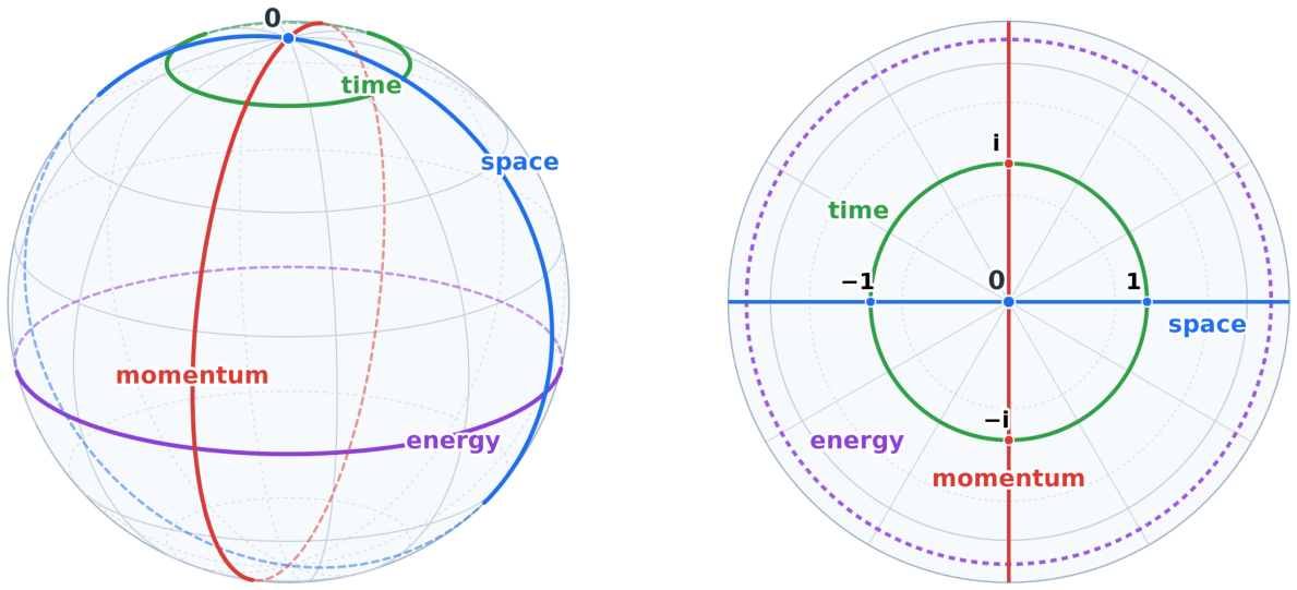
This section states what the operator layer of Section 3, Section 4, Section 5 and Section 6 is, in the geometry of the framed shell. The orbital shell of the frame carries two families of curves [21]: the meridians , the additive rays in the directions , and the latitude circles , the drive orbits at radius a. The additive Fourier pair (space, momentum) lives on two meridians — , the prime meridian in the direction of the unit, and , the quarter-turn meridian in the direction — and the multiplicative Fourier pair (time, energy) on two latitudes — , the drive’s own orbit through the unit, and , one capacity-step down the ladder, the first latitude past the equator. Both dualities are the same index advance by the capacity: , the quarter-turn on the meridian pair, and , the quarter-cycle on the latitude pair. We call motion along the latitudes zonal and motion along the meridians meridional. Figure 2 shows the four domains on the reference shell. The claims of this section are exact; their physical names are tagged identifications of the FRC programme.
Theorem 9
(The free evolution is the drive). Let be the phase cycle and let be the drive pullback, . Then:
- 1.
- D is unitary for the Hermitian form (10).
- 2.
- The multiplicative characters (k on the exponent cycle ) are a K-basis of eigenvectors, withthe winding-k mode acquires phase per chronon — the finite evolution kernel, with the energy read as the winding number; the characters are the shell’s plane waves, and the massive periods of 7 give the finite mass-shell reading.
- 3.
- Every character line is isotropic for the form except and , whose eigenvalues are exactly , the intersection of the norm-one torus with the split phase cycle.
Proof. (1) permutes ; reindex the defining sum. (2) ; the characters are linearly independent by Dedekind’s lemma. (3) The character values lie in and are Frobenius-fixed, so , which vanishes unless ; the exceptional eigenvalues are and , and since and force . □
To place interactions on the same space as the free evolution, equip with the cycle Laplacian of the drive,
which is self-adjoint (D is unitary with ), diagonal on the characters with Frobenius-fixed eigenvalues , and commutes with D. Cayley steps of Hamiltonians on then live in the same unitary group as the drive; the translation Laplacian of Section 3 lives on instead, the two spaces differing by the zero element — the seam between the additive and multiplicative pictures.
Corollary 9
(Two evolution sectors, one space). In the unitary group of there are two structurally distinct families: the split-phase sector — the drive and its powers, with spectrum in the phase cycle on isotropic character lines — and the norm-one sector — the Cayley propagators of Hamiltonians on , with scalar phases in for Frobenius-fixed spectra (Theorem 4; over splitting fields the phases lie in the corresponding norm-one tori, Remark 13). The two phase groups intersect in alone, so the free zonal evolution is not a Cayley step of any Hamiltonian with Frobenius-fixed spectrum: the continuum’s single unit circle appears here as two finite tori, the split cycle carrying the free (registration) kernel and the norm-one torus carrying the interacting (Cayley) and boost transports. Moreover the two sectors compose exactly: for H any polynomial in , , and is a unitary evolution with commuting free and interacting factors.
Proof.
The phases: immediate from Theorems 9 and 4 — a Cayley propagator of a Hamiltonian with spectrum in has scalar phases , while D has an eigenvalue of order . The composite: D commutes with , hence with every rational function of it, including ; a product of commuting unitaries is unitary. Machine-verified at : self-adjoint, , both factors unitary. □
7.0.0.1. Finite Plane Waves, Dispersion, and the Mass Shell.
The two sectors carry their spectral data very differently, and the difference is exact. On the zonal side the characters are the plane waves, and the cycle Laplacian has the closed dispersion relation
the finite band curve (the labelled continuum reading is ), whose Cayley phases populate . On the meridional side there are no plane waves at all: , so K contains no nontrivial -th root of unity and the translations admit no K-valued characters — the kinetic sector is unipotent, which is the operator form of the same fact. The mass shell follows: since is nilpotent, is invertible for every , so the static massive Dirac equation has only on the periodic coordinate shell. Mass is not a kernel condition in the finite register; it is an evolution phase — the norm-one factor of 7 — and the finite energy–momentum–mass relation is carried jointly by the factorization and the period law .
Remark 14
(The shell reading, tagged). With Theorem 9 beside the Dirac layer of Section 5, the two wave formalisms are the two Fourier pairs of one shell.Schrödinger dynamics is the exact zonal evolution: the drive circulates the time latitude , one packet per chronon; its spectrum is the winding ladder read a quarter-cycle down, at the energy latitude (Figure 2). General self-adjoint interactions enter through the norm-one sector as exact Cayley steps.Dirac dynamics is the exact meridional development: the operator is built entirely from translations, its equation balances meridional development rate against the winding rate m (Remark 11), and its covariance group is the boost torus transporting the zonal/meridional split (Lemma 5), with the time coordinate carried in the chronon-count chart on the translation cycle . The three tori of the shell thus hold the three dynamical seats — the free evolution, the meridional translations and kinetic periods, the interactions and boosts — and the light cone between the two developments is a square-class boundary, not a locus of registered motion (Theorem 2). Both dynamical sectors are isentropic in the exact sense of Remark 12: the wave dynamics of the shell neither creates nor destroys distinguishability, and compression is confined to the arithmetic (power-map) layer.
Remark 15
(Programme position). The ontological stance behind this reading treats the primary object as a finite symmetry space of algebraic possibilities, with every description — including the continuum Schrödinger–Dirac formalism — an incomplete projection of it [20]. On that stance, the theorems of this paper say that the projection loses nothing operator-theoretic: preservation, factorization, transport, and now the free evolution and its spectrum are exact at the finite level, and what the continuum adds is chart convenience, at the price of collapsing distinctions the finite register keeps (two unit circles, Corollary 9; two speed-of-light seats, Corollary 1). The theorems stand independently of the stance.
8. Discussion
The construction gives a finite operator layer over the framed shell. The Euclidean side uses as configuration space and K as coefficient field. The Lorentzian side uses as coordinate shell and the same coefficient field K for gamma matrices and spinors. The coordinate/coefficient split is essential: is written over , while the square root w of the nonsquare belongs to K — and the coefficient itself is canonical, , the drive multiplier, the frame’s one universally-nonsquare datum.
The Schrödinger-type results are an exact Cayley preservation theorem and the finite Cayley transform. A self-adjoint finite Hamiltonian generates a finite family of admissible Cayley maps, each preserving the Hermitian form exactly; the scalar Cayley map is a bijection from the Frobenius-fixed projective line onto the norm-one torus ; and the free evolution is the drive itself, exactly, with the winding number as energy (Theorem 9). Since the state space is finite, every trajectory is periodic, and the periods are classified by the shell’s tori: order for kinetic (unipotent) propagators, order dividing for potential (norm-one) propagators (Theorem 8). These are algebraic periodicity statements over a finite field, independent of any continuum spectral theorem.
The Dirac-type results are an exact Clifford, transport, and evolution construction. The gamma matrices encode the diagonal form , the finite Dirac operator factors to the spinorial Klein-Gordon operator, and the boost subgroup transports the standard operator to conjugate finite operators — the subgroup being the norm-one torus itself, by Hilbert 90 (Lemma 5). The symmetric Dirac operator is self-adjoint for the twisted spinor form of 7, so the Dirac sector carries exact unitary Cayley evolution with classified periods (7): -power massless periods, mass phases on . The covariance and evolution statements are equalities of finite operators on the same finite spinor-field set, with the transporting group shared with the evolution phases. The construction is deliberately in its boost content; the full finite orthogonal and spinorial family is left to the open problems.
The finite counts distinguish two algebraic behaviors. Cayley propagators and boost transports are bijections; shell power maps need not be. This is the finite-set content behind the loss factors. The packet, invariant, and fiber structure associated with shell changes is a separate finite-transfer problem.
The finite setting also fixes the level at which the operator identities live. The Hermitian form is a finite sum, the Hamiltonians and Dirac operators are endomorphisms of finite-dimensional K-spaces, Cayley preservation is a matrix identity whenever the denominator is invertible, and the Dirac-to-Klein-Gordon factorization is an exact equality of finite difference operators. This is the algebraic core carried by the construction.
This is the main consolidation supplied by the paper. The finite scheme does not approximate the continuum formalism by adding cutoffs; it isolates the part of the formalism that is already algebraic and makes it exact inside finite arithmetic — and it keeps distinctions the continuum collapses: the single unit circle splits into the split phase cycle and the norm-one torus (Corollary 9), and the single symbol splits into the registered two-way constant and the odd-parity one-way coefficient (Corollary 1). The statistical layer of the programme — the Born rule as registration count, measurement as shared-core comparison, exact composite recurrences — is developed in its companion quantum paper and rides on the operator identities proved here; the interface is one sentence: registered outcomes are counts over shared cores, computed with the same Hermitian pairings and unitary steps this paper constructs.
Several mathematical problems are now well posed. The first is the full period classification for mixed Hamiltonians: distribute the spectrum over the tori and , and determine the unipotent exponent a as a function of dimension and spinor structure (Remark 13 states the conjectured shape, an exact quintic instance, and the exponent formula to be tested). The second is to extend the explicit boost subgroup to larger finite orthogonal and spinorial families; the answer being structural (, Hilbert 90), the higher families should organise by the same torus data. The third is to connect the Dirac transport constructed here with packet-level invariants in the quadratic extension. The fourth is to formulate an observer-local coordinate derivation of the finite Dirac arena from the global shell geometry of [21].
9. Conclusion
For primes , the framed finite field carries a derived Euclidean phase element with . The Lorentzian coordinate form on depends only on the nonsquare class of its coefficient, whose canonical representative is the drive multiplier itself, ; the quadratic extension supplies Frobenius conjugation and spinorial coefficients. From these data one obtains exact finite analogues of Schrödinger and Dirac dynamics.
On Euclidean configuration spaces , finite Hamiltonians built from translations and finite potentials are self-adjoint, admissible Cayley transforms preserve the Hermitian form exactly, and the scalar Cayley map is a bijection from the self-adjoint projective line onto the norm-one torus . The free evolution is the drive itself: winding modes acquire phase per chronon, the winding number playing energy. On the Lorentzian coordinate shell , explicit gamma matrices over K satisfy the Clifford relations for , the finite Dirac difference operator factors into a spinorial Klein-Gordon operator, and the boost subgroup — the norm-one torus, by Hilbert 90 — admits an explicit spin lift and transports the Dirac operator by exact conjugation; the boost content is deliberately , the full finite spin family being future work. The symmetric Dirac operator is self-adjoint for a twisted spinor form forced by the Frobenius arithmetic, so the Dirac sector carries exact unitary Cayley evolution: -power massless periods, the mass phase on the norm-one torus. The worked shells and instantiate the two admissibility classes, the latter the minimal shell of the programme’s admissible congruences.
The resulting maps are finite and reproducible. Cayley propagators and boost transports are bijective, with orbit periods classified by the shell’s tori: for kinetic, for potential propagators. Shell power maps on compress by the exact arithmetic factor — an exact Hartley-entropy account in which the wave dynamics is isentropic and compression is purely arithmetic. Together the layers support one structural reading: Schrödinger dynamics is the exact zonal evolution of the framed shell and Dirac dynamics its exact meridional development — the two wave equations are the two Fourier pairs of one finite shell.
Reproducibility Map
The validation suite maps to the propositions one-to-one: finite_checks (Examples 1, 2, the power-map counts of Proposition 10, the Cayley admissibility and orders over all trace-zero parameters, the Clifford relations of Proposition 3, the conjugation formulas of Proposition 4, the transported family of Proposition 7, and a covariance sample for Corollary 5); o2_checks (Lemmas 1, 2, the square classes of every named residue on all symmetry-complete shells , and the admissibility anchors of Remark 4); o7_checks (Theorems 1, 2 and Corollary 1, with the drive-step parity exhaustive over every primitive root of the worked shells); o134_checks (Lemma 5 by exhaustive torus enumeration with the Hilbert-90 identity per element, Theorem 4, Theorem 8 with attained orders, and the quintic instance of Remark 13); latitude_checks (the latitude indices and terminal-latitude identities of Section 7); shell_checks (Theorem 9 exhaustively over all windings and cycle points, the sector separation of Corollary 9, and the numbers of Example 3); and o8_checks (Lemma 7 at including the failure of the -twist, Theorem 7 with the operator computation at — self-adjointness and unitarity as matrix identities, the massless -power period, the massive factorization — the commuting free–interacting composite of Corollary 9, the spin-lift/form transport of Proposition 8, and the cycle dispersion relation of Section 7). Every script runs in exact arithmetic — no floats, no random sampling — and every number quoted in the manuscript is reproduced by one of them.
Author Contributions
The sole author conceived and directed the research and takes full responsibility for every definition, statement, and argument herein. The development, proofreading and the verification of the claims, were carried out with assistance of an artificial-intelligence system.
Funding
This research received no external funding.
Data Availability Statement
No new empirical data were created or analysed in this study. The exact-arithmetic verification scripts are publicly available on GitHub.
Acknowledgments
The author thanks early readers for comments on earlier versions of this manuscript.
Conflicts of Interest
The author confirms no potential conflict of interest.
References
- Lidl, R.; Niederreiter, H. Finite Fields, 2 ed.; Cambridge University Press: Cambridge, UK, 1997. [Google Scholar] [CrossRef]
- Lam, T.Y. Introduction to Quadratic Forms over Fields. In Graduate Studies in Mathematics; American Mathematical Society: Providence, RI, USA, 2005; Vol. 67. [Google Scholar] [CrossRef]
- Taylor, D.E. The Geometry of the Classical Groups. In Sigma Series in Pure Mathematics; Heldermann Verlag: Berlin, Germany, 1992; Vol. 9. [Google Scholar]
- Chevalley, C. The Algebraic Theory of Spinors and Clifford Algebras. In Collected Works; Springer: Berlin, Germany, 1996; Vol. 2. [Google Scholar]
- Porteous, I.R. Clifford Algebras and the Classical Groups; Cambridge University Press: Cambridge, UK, 1995. [Google Scholar] [CrossRef]
- Crank, J.; Nicolson, P. A Practical Method for Numerical Evaluation of Solutions of Partial Differential Equations of the Heat-Conduction Type. Math. Proc. Camb. Philos. Soc. 1947, 43, 50–67. [Google Scholar] [CrossRef]
- Schwinger, J. Unitary Operator Bases. Proceedings of the National Academy of Sciences of the United States of America 1960, 46, 570–579. [Google Scholar] [CrossRef] [PubMed]
- Wootters, W.K. A Wigner-Function Formulation of Finite-State Quantum Mechanics. Ann. Phys. 1987, 176, 1–21. [Google Scholar] [CrossRef]
- Gibbons, K.S.; Hoffman, M.J.; Wootters, W.K. Discrete Phase Space Based on Finite Fields. Phys. Rev. A 2004, 70, 062101. [Google Scholar] [CrossRef]
- Lev, F.M. Introduction to a Quantum Theory over a Galois Field. Symmetry 2010, 2, 1810–1845. [Google Scholar] [CrossRef]
- Chang, L.N.; Lewis, Z.; Minic, D.; Takeuchi, T. Galois Field Quantum Mechanics. Mod. Phys. Lett. B 2013, 27, 1350064. [Google Scholar] [CrossRef]
- Chang, L.N.; Lewis, Z.; Minic, D.; Takeuchi, T. Spin and Rotations in Galois Field Quantum Mechanics. J. Phys. A Math. Theor. 2013, 46, 065304. [Google Scholar] [CrossRef]
- Schumacher, B.; Westmoreland, M.D. Modal Quantum Theory. Found. Phys. 2012, 42, 918–925. [Google Scholar] [CrossRef]
- Bialynicki-Birula, I. Weyl, Dirac, and Maxwell Equations on a Lattice as Unitary Cellular Automata. Phys. Rev. D. 1994, 49, 6920–6927. [Google Scholar] [CrossRef] [PubMed]
- Meyer, D.A. From Quantum Cellular Automata to Quantum Lattice Gases. J. Stat. Phys. 1996, 85, 551–574. [Google Scholar] [CrossRef]
- Strauch, F.W. Relativistic Quantum Walks. Phys. Rev. A 2006, 73, 054302. [Google Scholar] [CrossRef]
- D’Ariano, G.M.; Perinotti, P. Derivation of the Dirac Equation from Principles of Information Processing. Phys. Rev. A 2014, 90, 062106. [Google Scholar] [CrossRef]
- Bisio, A.; D’Ariano, G.M.; Tosini, A. Quantum Field as a Quantum Cellular Automaton: The Dirac Free Evolution in One Dimension. Ann. Phys. 2015, 354, 244–264. [Google Scholar] [CrossRef]
- Carroll, S.M. Completely Discretized, Finite Quantum Mechanics. Found. Phys. 2023, 53. [Google Scholar] [CrossRef]
- Akhtman, Y. Relativistic Algebra over Finite Ring Continuum. Axioms 2025, 14, 636. [Google Scholar] [CrossRef]
- Akhtman, Y. Geometry and Constants in Finite Ring Continuum. Symmetry 2026, 18. [Google Scholar] [CrossRef]
- Akhtman, Y. Euclidean-Lorentzian Dichotomy and Algebraic Causality in Finite Ring Continuum. Entropy 2025, 27, 1098. [Google Scholar] [CrossRef] [PubMed]
- Hartley, R.V.L. Transmission of Information. Bell Syst. Tech. J. 1928, 7, 535–563. [Google Scholar] [CrossRef]
- Rényi, A. On Measures of Entropy and Information. In Proceedings of the Proceedings of the Fourth Berkeley Symposium on Mathematical Statistics and Probability, Berkeley, CA, USA, 1961; Vol. 1, pp. 547–561. [Google Scholar]
- Landauer, R. Irreversibility and Heat Generation in the Computing Process. IBM J. Res. Dev. 1961, 5, 183–191. [Google Scholar] [CrossRef]
- Bennett, C.H. Logical Reversibility of Computation. IBM J. Res. Dev. 1973, 17, 525–532. [Google Scholar] [CrossRef]
- Fredkin, E.; Toffoli, T. Conservative Logic. Int. J. Theor. Phys. 1982, 21, 219–253. [Google Scholar] [CrossRef]
- Shannon, C.E. A Mathematical Theory of Communication. Bell Syst. Tech. J. 1948, 27, 379–423, 623–656. [Google Scholar] [CrossRef]
Figure 1.
The framed shell . Left: the orbital 2-sphere — observer origin 0 at the north pole, the additive prime meridian (blue), the quarter-turn meridian (red), the multiplicative latitudes (green) forming the phase cycle . Right: the framed-complex chart — the prime meridian as the real axis, the quarter-turn meridian as the imaginary axis, the latitudes as norm circles. All marks are frame data.
Figure 1.
The framed shell . Left: the orbital 2-sphere — observer origin 0 at the north pole, the additive prime meridian (blue), the quarter-turn meridian (red), the multiplicative latitudes (green) forming the phase cycle . Right: the framed-complex chart — the prime meridian as the real axis, the quarter-turn meridian as the imaginary axis, the latitudes as norm circles. All marks are frame data.
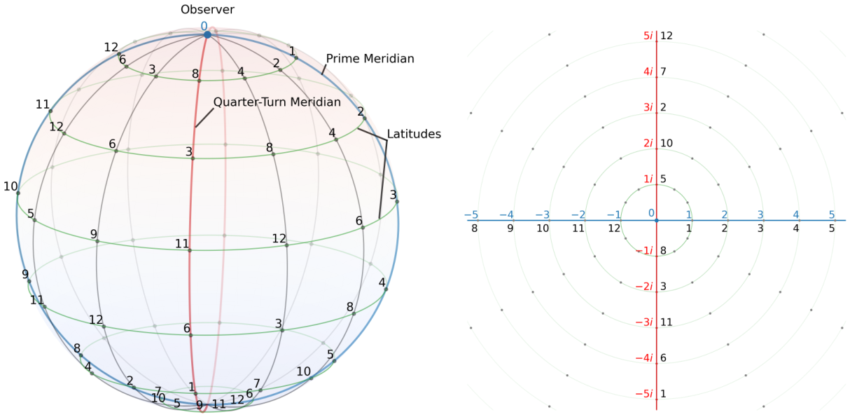
Figure 2.
The four representation domains of one framed shell ( as the reference shape): space (blue, the prime meridian ) and momentum (red, the quarter-turn meridian ) are the additive-Fourier (meridional) pair; time (green, the latitude ) and energy (purple, the latitude ) are the multiplicative-Fourier (zonal) pair, the drive running along time. All marks are frame data. Left: the orbital sphere, origin at the pole. Right: the same data flattened into the observer’s chart.
Figure 2.
The four representation domains of one framed shell ( as the reference shape): space (blue, the prime meridian ) and momentum (red, the quarter-turn meridian ) are the additive-Fourier (meridional) pair; time (green, the latitude ) and energy (purple, the latitude ) are the multiplicative-Fourier (zonal) pair, the drive running along time. All marks are frame data. Left: the orbital sphere, origin at the pole. Right: the same data flattened into the observer’s chart.
Disclaimer/Publisher’s Note: The statements, opinions and data contained in all publications are solely those of the individual author(s) and contributor(s) and not of MDPI and/or the editor(s). MDPI and/or the editor(s) disclaim responsibility for any injury to people or property resulting from any ideas, methods, instructions or products referred to in the content. |
© 2026 by the authors. Licensee MDPI, Basel, Switzerland. This article is an open access article distributed under the terms and conditions of the Creative Commons Attribution (CC BY) license (http://creativecommons.org/licenses/by/4.0/).
Copyright: This open access article is published under a Creative Commons CC BY 4.0 license, which permit the free download, distribution, and reuse, provided that the author and preprint are cited in any reuse.