
Submitted:
15 October 2025
Posted:
21 October 2025
You are already at the latest version
Abstract
Health impact due to population exposure to PM2.5 shows that the densely populated suburbs surrounding the urban core have the largest impact in terms of mortality. Health impact due to air pollution is higher in January (dry season) with estimated 625 deaths and 124 cardiovascular diseases (cvd) hospitalization as compared with estimated 94 deaths and 18 cvd hospitalization in July (wet season). One of the research questions posed by the city authority is whether converting diesel buses to electric buses can yield environmental and health benefits. Our work shows that the scenario of replacing 50% of fossil fuel combustion buses with electric buses does not yield perceptible change in mortality health effect. This is due to emission from buses is small as compared to those from the whole transport sector and other sectors. This study emphasizes the need for integrated, targeted emission control strategies to address spatial and temporal variability in pollution. The findings offer valuable insights for policymakers to develop effective measures in urban planning for improving air quality and protecting the health of people in Hanoi.
Keywords:
air pollution
; health impact
; traffic emission
; fossil fuel
; electric vehicles
; reduction scenarios
; PM2.5
1. Introduction
Air pollution is one of the most serious environmental problems in urban areas. The World Health Organization (WHO) has estimated that air pollution causes the death of more than 8 million people per year in the world, among that there are more than 70% people death per year in developing countries. Millions of people are found to be suffering from various respiratory illnesses related to air pollution in large cities. Therefore, urban air quality management should be urgently considered in order to protect human health. Air quality in developing countries has deteriorated considerably, exposing millions of people to harmful concentrations of pollutants because urban air quality management has not been adopted for a variety of difficulties.
The sources of air pollution can be categorized by their origins, primary or secondary pollutants, stationary or mobile sources, point sources or area sources …. The United States Environmental Protection Agency (US EPA) commonly classifies sources of air pollution by splitting them into two main categories: anthropogenic and natural sources.
Anthropogenic air pollution originates from large stationary sources (e.g., industries, power plants, and municipal incinerators), small stationary sources (e.g., households and small commercial boilers), and mobile sources (e.g., traffic). In addition, anthropogenic sources can be classified into two main source groups: Stationary sources, which are point sources and non-point (Area) sources, and mobile sources, which are on-road and non-road (off-road). Stationary sources include smokestacks of power plants, manufacturing facilities (factories), waste incinerators, furnaces, and other fuel-burning heating devices. Traditional biomass burning is the primary source of air pollutants in developing and poor countries. Traditional biomass includes wood, crop waste, generating NOx, SO2, PM, and CO2. Mobile sources include motor vehicles, marine vessels, and aircraft. In cities, transportation is known as the primary source of air pollution. Along with congestion and large, poorly maintained vehicle fleets pollute air quality in cities.
Air pollution is increasingly problematic in Vietnam due to rising emissions from industrial growth. The country’s reliance on fossil fuels has intensified pollution in recent years, particularly in major cities like Hanoi and Ho Chi Minh City [1,2]. Reports indicate that Hanoi’s annual PM10 and PM2.5 levels often exceed local air quality standards [3] . Key contributors to this pollution include the combustion of coal, oil, and natural gas [4] . Despite Vietnam’s commitment to reducing greenhouse gas emissions through renewable energy by 2030 as in nationally determined contributions (NDC, 2015), ongoing reliance on fossil fuels is expected to persist, potentially increasing emissions over the next decade [5] .
Hanoi, the capital city of Vietnam, has undergone significant urban growth, leading to the conversion of agricultural land into urban areas and an associated rise in pollution from traffic, industry, and residential activities [6] . This rapid development has resulted in increased levels of air pollutants, such as nitrogen dioxide (NO₂) and sulfur dioxide (SO₂), particularly in newly urbanized zones [7]. Pollutant concentration from roadside emission from traffic in Hanoi streets had been modelled using the Operational Street Pollution Model (OSPM) [7] . The predictions from five streets were evaluated against measurements of NOx, SO2), CO, and benzene (BNZ). Calibration of the model was used to calculate the average emission factors of the vehicle fleet for various pollutants. Traffic emissions are a significant source of air pollution, with studies showing that particulate matter (PM₁₀) from transportation contributed to thousands of premature deaths in previous years [1] . Additionally, roadside air pollution presents serious health risks for the city’s population [8]. To address these pressing issues, evaluating air quality in Hanoi, focusing on seasonal changes and the potential impact of reducing traffic emissions, is crucial for implementing effective pollution control measures. Air quality dispersion model on the regional scale such as WRF-Chem (Weather Research Forecast – Chemistry) or WRF-CMAQ (Weather Forecast – Community Multiscale Air Quality) model is used by many authors in various countries to assess the impact of emission from various sources on air quality in the domain under consideration [9,10,11,12]
This study aims to assess air quality in Hanoi (Vietnam) using the Weather Research Forecast - Community Multiscale Air Quality (WRF-CMAQ) model and evaluate air pollution reduction for two emission scenarios. Health impact due to population exposure of PM2.5 air pollutants as simulated from the model will be assessed for the emission scenarios. This study uses the updated emission inventory for thermal power plants, analyzing a variety of pollutants and changes over recent years in Hanoi. This study sets up a meteorological model and simulates air pollution dispersion for Hanoi, calibrating and validating the model. Then, we simulate the dispersion of air pollutants using the photochemical model based on the current and reduced emission scenarios, thereby assessing the impact of road traffic sources on air pollution in Hanoi.
2. Data and Methods
2.1. Emission Inventory in Hanoi
In this study, air emission inventory results were the input of the CMAQ model. We calculated air emission sources based on three main categories: line source, area source, and point source.
2.1.1. Line Source
The EMISENS model is used to calculate emissions from road transportation activities. This study classified streets into five categories: highways, rural roads, urban streets, suburban streets, and industrial streets (located in the industrial zone) [13]. Meanwhile, vehicles were divided into five types: buses/coaches, heavy-duty vehicles (HDVs) with a total gross weight of over 3.5 tonnes, light-duty vehicles (LDVs) which weigh less than 3.5 tonnes, cars (<15 seats), and motorcycles.
The study referenced the number of vehicles in 2022 and surveyed 200 extra questionnaires on 15 streets. Directly interview and collect information directly from vehicle owners for each type of vehicle on each specific road.
2.1.2. Area and Point Sources
We used emissions factors and activity data as the equation below
E = EFs x A x (1-ER/100)
where:
E is emissions (typically in tons/year),
A is activities rate (amount of fuel use, capacity, or number of products)
EF is emission factors (related to A),
ER is emission reduction efficiency (only if abatement devices are used).
For point sources, the key industrial products in Hanoi in 2022 include six products from the mechanical and manufacturing industry (accounting for 18.2%), four products from the electrical and electronic industry (accounting for 12.1%), five products from the information technology industry (accounting for 15.2%); 8 products of the textile, garment, and footwear industry (accounting for 24.2%); 4 products of the agricultural and food processing industry (accounting for 12.1%); 3 products of the chemical, rubber, plastic and pharmaceutical industries (accounting for 9.1%); 2 products of the construction materials industry (accounting for 6.1%) and 1 product of the handicraft industry (accounting for 3%) [18]. CNG was the most significant fuel used in industry, especially in chemical chemistry. The other fuels including oil types (DO, FO, and cashew oil), gasoline, wood and wood products, and coal are used for industry.
Area sources, such as households, restaurants, construction material stores, pagodas, and biogenic sources (straw burning), are calculated.
The sources of EFs considered were referenced from the emission inventory guidebook of the European Environment Agency (EEA) [19,20,21]
2.2. WRF-CMAQ Model
The WRF (Weather Research and Forecasting)-CMAQ model (version 5.3.1, US EPA, 2019) was employed to simulate atmospheric processes using the CB6 (Carbon Bond 6) chemical mechanism. The CB6 mechanism provides a detailed representation of atmospheric chemical reactions, particularly those involving secondary organic aerosol formation [22,23]. The WRF model was first executed to generate meteorological input data for CMAQ using the Meteorology-Chemistry Interface Processor (MCIP).
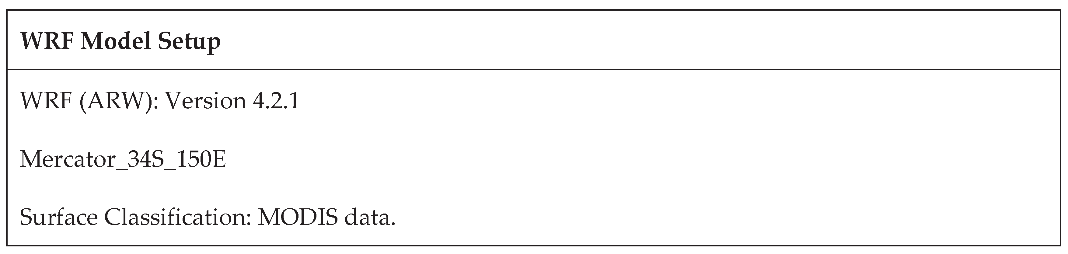
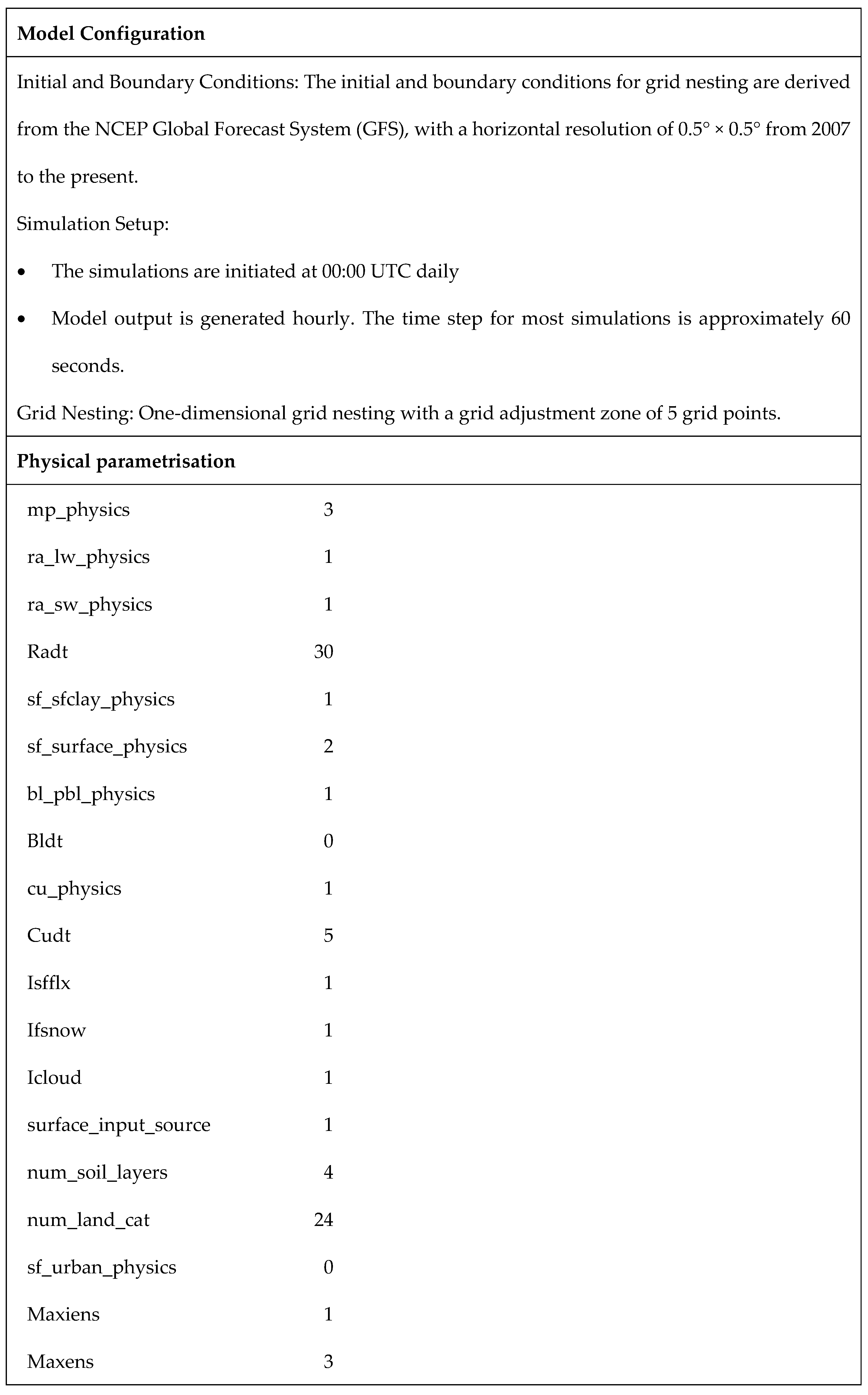
Domain configuration and physics/chemistry options for WRF are detailed in Figure 1 and Table 1. Meteorological data were obtained from the Global Forecast System (GFS) by the National Centers for Environmental Prediction (NCEP). GFS integrates four sub-models (atmosphere, ocean, land/grid, and sea ice) to provide high-resolution forecasts of variables such as temperature, wind, precipitation, soil moisture, and atmospheric ozone.
The WRF-CMAQ simulation employed three nested domains to capture spatial variability across scales. The outermost domain (D1) consisted of a 42 × 42 grid with a horizontal resolution of 27 × 27 km, covering northern and north-central Vietnam, the East Sea, and parts of Laos, Thailand, and China. The second domain (D2) featured a 40 × 43 grid with a resolution of 9 × 9 km, focusing on northern and north-central Vietnam and adjacent regions in Laos and China. The innermost domain (D3) included a 43 × 43 grid with a 3 × 3 km resolution, encompassing Hanoi city and nearby provinces such as Thai Nguyen. This setup ensured high spatial resolution for the areas of interest while accounting for regional-scale meteorological dynamics.
Initial and boundary conditions for chemical species were sourced from the global CAM_Chem model (Community Atmosphere Model—Chemistry), available at NCAR (https://www.acom.ucar.edu/cam-chem/cam-chem.shtml). Anthropogenic emission data were provided by the research team’s 2022 emission inventory for Hanoi. The simulation period covered January and July 2022, representing the winter and summer seasons. Emission data from various sources and formats were processed into CMAQ-compatible inputs using a set of custom-developed Python scripts.
Post-processing tools, including Combine, Sitecmp, Writesite, Panoply, and QGIS, were utilized to analyze and validate the WRF-CMAQ simulation outputs. These tools enabled efficient extraction, organization, and comparison of modeled data with observational datasets, ensuring robust evaluation of the model’s performance in predicting air quality and atmospheric chemical composition.
2.3. Calibration and Validation for the WRF-CMAQ Model
The model performance was evaluated using statistical indices such as the Mean Bias (MB), Root Mean Square Error (RMSE), Mean Absolute Gross Error (MAGE), Index of Agreement (IOA), and Pearson Correlation Coefficient (R). In addition, the Factor 2 coefficient and Standard Deviation (SD) were also used [24] .
The Mean Bias (MB) is calculated as follows:
MB = P ̅ - O ̅ (Equation 1)
where P ̅ is the average value of the model results and O ̅ is the average value of the observed data. An MB value greater than 0 indicates an overestimation of the simulated data, while an MB value less than 0 indicates an underestimation.
The Normalized Mean Bias (NMB) is used as a normalization method to facilitate the analysis across a range of concentration levels. This statistic calculates the average difference between the model and observations relative to the total observed values. NMB is a useful model performance index as it prevents excessive inflation of the observed value range, especially at lower concentration levels. The Normalized Mean Bias is defined as follows:
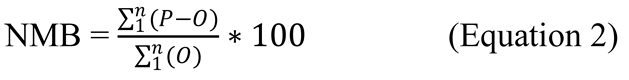
where: Pi represents the model values, Oi represents the observed values, and N is the total number of samples.
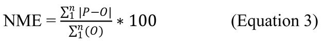
The Normalized Mean Error (NME) is similar to the NMB, in which the perfomance statistic is used to normalize the mean error. NME calculates the absolute value of the difference between the model and the observations relative to the total observed values. The Normalized Mean Error is defined as follows:
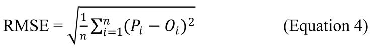
The RMSE (Root Mean Square Error) represents the total error of the model and is equal to zero in ideal cases.
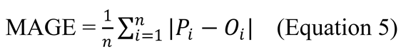
MAGE (Mean Absolute Gross Error) calculates the mean absolute error between simulated values and observed measurements, reflecting the average similarity of simulation errors. Similar to RMSE, lower MAGE values indicate better agreement between the observed data and the model results
The Index of Agreement (IOA) provides a sophisticated measure of model performance. IOA is a dimensionless parameter with values ranging from -1 to 1, where 1 indicates an ideal model. A value of 0 signifies that the total error of the model is equal to the sum of the deviations of the observations from their mean value. A value of 0.5 indicates that the total error of the model accounts for half of the deviations between observed values and their mean. The constant variable c is related to the frequency of model output and is assigned a value of 2 (Josh et al., 2018). The variable Pi represents the predicted value at time point (i), while Oi represents the observed value at the same time point (i), and O̅ represents the mean of the observed values.
Pearson’s correlation coefficient is a measure of the linear relationship between simulated and observed data. Its value is zero when there is no correlation and increases as the coefficient approaches -1 or +1. Values close to +1 indicate a strong positive correlation between the two variables.
 (Equation 8)
The Factor2 coefficient calculates the ratio between the simulated data (Pi) and the observed data (Oi), indicating the percentage of data that falls within the range of 0.5 ≤ Pi / Oi ≤ 2. Clearly, its optimal value is 1.
2.4. Population Exposure and Health Impact
The population exposure to air pollutants, especially PM2.5, and its impact on population health is an active area of epidemiological research in public health. To assess the risk, the relative risk (RR) factor is usually used to determine air pollution impact on health. The World Health Organization’s (WHO) Health Risks of Air Pollution in Europe project (HRAPIE) has recommended concentration-response functions for different health endpoints such as mortality (all cases) and cardiovascular (cvd) diseases for PM2.5 [25] (WHO, 2013).
These RR of each of the health endpoints for a 10μg/m3 increase of PM2.5 on mortality (all cases) and cardiovascular diseases hospitalization are
RR (mortality) = 1.0123 (CI: 1.0045, 1.0201)
RR (cvd) = 1.0091 (CI: 1.0017, 1.0201)
where CI is the confidence interval at a 95% level.
The HRAPIE relative risk for mortality value above means that a 10μg/m3 increase of PM2.5 would increase the mortality of the exposed population by 1.23% (CI: 0.45%, 2.01%). Similarly, an increase of 0.9% (CI: 0.17%, 2.01%) for cvd hospitalization for each increase of 10μg/m3 in PM2.5 concentration.
As in the previous studies, such as [26] , in this study, these recommended short-term concentration response coefficients for mortality and cvd disease hospitalization are used to assess the population health impact due to PM2.5 under different emission scenarios.
From the RR, the impact factor (IF) is then calculated to determine the impact associated with a specific change in air pollution concentration ΔX which is the PM2.5 concentration increase due to a emission change, and IF is calculated as:
IF = RRΔX/10 (Equation 9)
Equation (9) is a log-linear model which states that the logarithm of the impact factor (or relative risk function) is linearly changed with a change in ambient PM concentration.
And finally, the attributable number of the impact on health endpoint due to an increase of ΔX concentration in a population with a specific incidence rate for this endpoint is
AN = (IF-1) × Population × incidence rate (Equation 10)
The above Equations (9) and (10) are used by the US EPA to estimate the health impact due to changes in air quality in the United States [27] and implemented in the BenMAP v1.5 software tool. They are also used by many authors to assess the health impact of air pollution in various countries [28,29,30].
The population data used in this study is the 2019 high resolution population 1km by 1km dataset from the UN Humanitarian Data Exchange in TIFF format. The incidence rate is based on The Global Health Data Exchange (GHDx) from the Institute for Health Metrics and Evaluation (IHME) available from 1990 to 2019 (http://ghdx.healthdata.org, accessed 25 August 2025). According to GHDx data for 2019, the total number of deaths in Vietnam is 631,817 (CI: 538,099, 714,078). The corresponding population and mortality incidence rates Vietnam is derived as (96,372,928; 0.65%).
For the incidence rate of cvd hospitalization in Vietnam, there is currently no data publicly available that we can find. We use the figure similar to the figure of the heart failure (HF) hospitalization rate in Thailand of 168 per 100,000 in 2013 as provided by [31]
The population data at 1km x 1km resolution is converted to Netcdf file and then interpolated to the PM2.5 modelling domain. Population exposure and attributable number of people affected are then calculated from Equations (2) and (3).
The relative risk as a percentage of increase in risk implies that a reference value of PM2.5 is required. This reference value could be determined by either using the lowest value of PM2.5 where there is no effect on population health. The Global Exposure Mortality Model (GEMM), developed by [32], defined the minimum observed PM₂.₅ level in the cohort data as 2.4 µg/m³ below which no effect on mortality. This study is frequently used in global burden assessments. The other value that can be used is the so-called Theoretical Minimum-Risk Exposure Distribution (TMRED) that was proposed by Lim et al. 2012 in the Global Burden of Disease GBD 2010. This value is defined based on the lowest and 5th percentile of PM₂.₅ concentrations observed in major cohort studies from 5.8 to 8.8 µg/m³. In this study we use the WHO value of 5 µg/m³ recommended as a safe level or a reference value below which there is no impact on population health. There are other studies which showed that there is no safe level of PM2.5. But zero PM2.5 level is not real and a practical approach is to use the WHO guideline value.
To calculate health impact due to different scenarios, such as the city authority proposed on vehicle emission fleet having a percentage of electric vehicles (EV) as compared to one with no EVs, we can determine the relative impact between these scenarios without having to use the reference value such as WHO value. Simply use Equations (1) and (2) where ΔX is the change in PM2.5 concentration between the base case emission scenario without EVs and the scenario with EVs in the fleet. In our study, the daily mean of PM2.5 as predicted by WRF-CMAQ at each of the cells in the domain and the population within the same cell represents the exposure and hence the effect on health (mortality) will be calculated. We calculate the effect of PM2.5 on mortality in Hanoi modelling domain.in January (representing dry season) and July (representing wet season) and the corresponding changes in mortality effects when compared between the baseline emission and the scenario when 50% of fossil-combustion buses are replaced with electric buses.
3. Results and Discussion
3.1. Development of Input Emission Datasets for the CMAQ Model
This study used emission inventory results as the input data for the CMAQ model. The summary of Hanoi’s emission sources in 2022 is presented in Table 2 and Figure 2. Overall, traffic line sources accounted for the most significant emissions of all pollutants. The line source accounted for 92.9%, 97.9%, 34.2%, 92.4%, and 92.9% of NOx, CO, SO2, NMVOC, and CH4. Industrial activities contributed 59.9%, 10.1%, and 11.6% of total SO2, PM2.5 and PM10 emissions in Hanoi. The area sources accounted for 28,1% of TSP, 15.2% of PM2.5, and 19.6% of PM10 in Hanoi, whereas others were negligible sources.
3.2. Development of Emission Reduction Scenarios
In this study, alongside simulating air quality for two representative periods representing the rainy and dry seasons in Hanoi for the current state (2022), an emission reduction scenario was also developed to assess the potential for improving air quality by reducing emissions from one type of traffic sources. Specifically, in the reduction scenario (Scenario 2), it is assumed that 50% of the fossil fuel-powered public buses operating in the city are replaced by electric buses. Currently, there are 2,094 public buses operating in Hanoi. By 2030, around 1,047 electric buses are projected to replace traditional buses, representing approximately 2% of the total number of buses and coaches in the city. The emission data was adjusted according to Scenario 2 and then integrated into the CMAQ air quality model. The simulation results from Scenario 2 are compared with the baseline scenario (Scenario 1), as presented in the previous sections. The differences in the concentrations of key pollutants between the two scenarios will provide detailed information on the effectiveness of the traffic emission reduction measures in improving urban air quality.
Table 3 and Table 4 present detailed data on pollutant emissions for both simulation scenarios. In Scenario 2, the substitution of 50% of fossil fuel-powered buses with electric buses leads to a reduction in emissions ranging from 11.32% to 17.27% for key pollutants. Among these, carbon monoxide (CO) demonstrates the most significant reduction, while particulate matter (PM2.5) shows the most minor decrease. However, when evaluating total emissions from all traffic sources, the reduction in Scenario 2 relative to Scenario 1 is relatively modest, with a range of 0.01% to 3.3%. Notably, NOx exhibits the most considerable reduction, at 3.3%. These findings suggest that while introducing electric buses effectively lowers local emissions from this specific source, its impact on the overall reduction in emissions across all traffic sources is limited. It highlights the necessity for supplementary strategies to substantially reduce emissions within urban traffic sectors.
3.3. Model Calibration and Validation of CMAQ
Temperature validation involved extracting values at a height of 2 meters from the Time Series (TS) output files corresponding to the measurement location at Ha Dong station. Since the simulated temperature was provided in Kelvin, these values were converted to Celsius for comparison with observed data. Table 2 presents the comparison results between simulated and observed temperature values. A strong correlation (R = 0.89, Table 2) was observed between the simulated and observed temperature data. The test results indicated that the simulated temperatures met the MAGE and Factor 2 criteria (Table 5), suggesting that the model accurately reflected surface temperature changes during the validation period.
For wind validation, wind speed components in the x and y directions were extracted from the TS output files at a height of 10 meters. These components were then used to calculate the total wind speed and direction. The MAGE indices for wind speed at Ha Dong station met the standard values. The correlation coefficient (R) was 0.59, indicating that the WRF model more accurately reflected surface wind conditions. However, observed data at the station was limited to rounded wind speed and direction values recorded at specific times (1:00, 7:00, 13:00, and 19:00 LCT), restricting statistical comparison. Therefore, wind validation was further conducted by comparing wind rose diagrams and analyzing prevailing wind direction from WRF model output. Figure 3 shows the wind rose diagrams for observed and simulated data at Ha Dong station. A significant similarity in both wind speed and direction distributions was found. Both the WRF model and observations indicated a dominant southwest wind direction during the study period.
For CMAQ result validation, PM2.5 values were extracted from the CCTM-AELMO output file at the U.S. Embassy station in Hanoi. The CMAQ model demonstrated strong performance in simulating PM2.5 concentrations, with a R-value of 0.78 (Figure 4), MB of 0.64, and RMSE of 8.99. Additional performance metrics, including the IOA = -0.5, NMB = 7.11%, and NME = 28.51%, all met the U.S. EPA performance criteria (NMB ≤ ±30%, NME ≤ ±70%). These results indicate that the CMAQ model configuration used in this study is reliable and suitable for simulating air quality in northern Vietnam.
3.4. Air Quality Simulation Results in Hanoi
3.4.1. Temporal Distribution of Air Pollutants in Hanoi
Table 6 summarizes the average concentrations of air pollutants derived from the CMAQ model outputs for January and July 2022, specifically focusing on the northern region, particularly domain D3.
The temporal air quality analysis in Hanoi reveals substantial seasonal variations influenced by meteorological conditions and emission dynamics. In January 2022, pollutant concentrations were significantly higher compared to July 2022, as shown in Table 6. During winter, meteorological conditions such as low temperatures, stable atmospheric layers, and reduced vertical mixing limit pollutant dispersion. It leads to the accumulation of pollutants, particularly PM₂.₅, which exhibited an average concentration nearly six times higher in January than in July. Similarly, CO, NO₂, O₃, and SO₂ concentrations increased by factors of 1.9, 1.8, 1.3, and 2.3 during the winter months. These elevated levels reflect the impact of local and regional emission sources and unfavorable weather conditions.
Despite the seasonal increase in pollution, the average concentrations of some pollutants in January remained within the regulatory limits of QCVN 05:2023/BTNMT. For instance, the average CO concentration was recorded at 1861.8 ± 1535.1 µg/m³, approximately 5.4 times below the standard, while NO₂ and SO₂ concentrations were about 3.3 and 10 times below their respective limits. The average O₃ concentration, at 59.2 ± 10.6 µg/m³, was approximately half of the regulatory threshold. These findings suggest that while pollution levels are higher in winter, they generally comply with Vietnamese air quality standards.
In contrast, the summer season presented a markedly different scenario. Air quality in July 2022 was classified as good, primarily due to favorable meteorological conditions. Prevailing air masses from the ocean, high humidity, and enhanced precipitation facilitated the washout of atmospheric pollutants. This washout effect, combined with cleaner marine-origin air masses, significantly reduced pollutant concentrations. Specifically, PM₂.₅ concentrations decreased substantially, highlighting the influence of precipitation on fine particulate matter removal. CO, NO₂, O₃, and SO₂ concentrations also declined, reflecting reductions in both local emissions and regional contributions. The seasonal variation underscores the critical interaction between emission sources and meteorological factors, providing insights for developing targeted air quality management strategies
3.4.2. Spatial Distribution of Air Pollutants in Hanoi
The spatial distribution of air pollutants in Hanoi highlights distinct patterns across different regions, shaped by the interplay between emission sources, topography, and atmospheric processes. PM₂.₅ concentrations, as illustrated in Figure 5, were significantly higher in suburban areas compared to central urban regions. These elevated levels in the outskirts of Hanoi are linked to contributions from industrial activities and cross-boundary pollutant transport. We also study the backward trajectory analysis (BWT) which indicates air masses moving from the northern part of Vietnam carried pollutants from industrial zones into Hanoi, exacerbating PM₂.₅ pollution in suburban areas. It highlights the role of regional emissions and long-range transport in fine particulate matter accumulation.
In contrast, urban areas exhibited lower PM₂.₅ concentrations, which could be attributed to enhanced dispersion facilitated by urban heat island effects and lower contributions from distant sources. However, urban regions showed higher concentrations of gaseous pollutants such as CO, NO₂, and SO₂ (Figure 6, Figure 7 and Figure 8). These pollutants are closely associated with local emission sources, including traffic, industrial operations, and residential combustion activities. High traffic density, particularly during peak hours, contributes significantly to CO and NO₂ levels, while fossil fuel combustion in industries adds to SO₂ emissions. The concentration of O₃, a secondary pollutant, showed a more complex spatial pattern (Figure 9), influenced by photochemical reactions and precursor emissions from local and regional sources.
The spatial differentiation between PM₂.₅ and gaseous pollutants underscores the distinct mechanisms driving their formation and distribution. While PM₂.₅ pollution is primarily influenced by distant sources, chemical transformations, and accumulation under stable atmospheric conditions, gaseous pollutants are more strongly dependent on localized emission dynamics. Additionally, the presence of fine and coarse particulate matter in suburban areas suggests the contribution of secondary atmospheric reactions, further complicating the pollution landscape.
These spatial and temporal findings emphasize the importance of a comprehensive air quality management strategy for Hanoi. Addressing local emission sources in urban areas is critical to controlling CO, NO₂, and SO₂ concentrations while mitigating PM₂.₅ pollution requires regional cooperation to reduce industrial emissions and manage transboundary pollution. By integrating meteorological considerations and emission control policies, Hanoi can achieve sustainable improvements in air quality and reduce the health risks associated with air pollution.
3.5. Evaluation of Air Quality Simulation Results with Emission Reduction Scenarios
Table 7 presents the difference ratio of average Air Pollutant concentrations for January and July between the two scenarios for domain 3, as calculated from the CMAQ simulation outputs.
Implementing emission reduction measures in Hanoi in January 2022 demonstrated varying levels of effectiveness across different pollutants, as shown by CMAQ model simulations. The concentration differences between the scenarios are summarized in Table 4. The results indicate that bus emission reductions led to concentration changes ranging from approximately -1.9% to 2.96%. However, the overall effectiveness in January was limited, primarily due to unfavorable meteorological conditions, including low temperatures and a shallow boundary layer, facilitating the accumulation of pollutants at the surface. Additionally, long-range pollutant transport from industrial zones in the northern region and beyond significantly influenced air quality in Hanoi, reducing the impact of local mitigation measures.
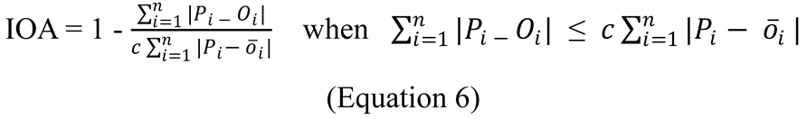
Figure 10.
Map of PM2.5 Concentration Difference Ratio between two scenarios for (a) January, (b) July across Domain 3.
Figure 10.
Map of PM2.5 Concentration Difference Ratio between two scenarios for (a) January, (b) July across Domain 3.
PM2.5 concentration differences showed minimal changes, with an average difference of 0.017% ± 0.041%, ranging from -0.064% to 0.088%. Spatial analysis (Figure 9a) revealed higher reductions in central Hanoi, where traffic emissions are most concentrated. It indicates that traffic-focused measures moderately reduced PM2.5 levels in urban centers. However, the reduction effect was less evident in suburban areas, highlighting the necessity for more comprehensive strategies to manage PM2.5 across the entire region.
For NO2, emission reduction measures achieved a more pronounced effect, with an average concentration reduction of 2.964% ± 0.332%, ranging from 1.592% to 3.420%. It underscores the critical role of controlling traffic emissions in mitigating NO2 pollution. In contrast, SO2 exhibited a modest average reduction of 0.068% ± 0.028%, ranging from -0.075% to 0.158%. The limited decrease in SO2 likely reflects the influence of secondary emissions and atmospheric transport processes. Spatial distribution patterns of NO2 and SO2 reductions (Figure 11a and Figure 12a) suggest shared sources, primarily from traffic emissions, in urban and suburban areas.
CO concentrations showed minor reductions, with an average decrease of 0.007% ± 0.002%, ranging from 0.002% to 0.010%. It indicates a consistent but limited impact of emission reductions on CO levels (Figure 13). Conversely, O₃ concentrations experienced a modest increase under Scenario 2, with an average difference of -1.959% ± 0.664%. The increase from -5.558% to -0.831% can be attributed to reduced NOₓ emissions. In urban environments with high NOₓ levels, NO acts as an O₃ scavenger. Reducing NOₓ emissions diminishes this effect, causing localized increases in O₃ concentrations, particularly in areas previously dominated by high NOₓ levels. Figure 14a illustrates these spatial differences, showing significant increases in central Hanoi.
In July 2022, the application of emission reduction measures led to more substantial reductions compared to January. Concentration difference rates ranged from -0.27% to 3.1%, reflecting the influence of favorable summer meteorological conditions. PM2.5 concentrations decreased by an average of 0.3387% ± 2.8198%, ranging from -5.2564% to 5.1372%. The reduction was more pronounced in urban areas, as shown in Figure 10b, where traffic-related emissions dominate.
NO2 reductions in July were notably higher, with an average rate of 3.1496% ± 0.2045%, ranging from 1.9106% to 3.7838%. Enhanced dispersion and washout effects during summer amplified the effectiveness of emission reductions. CO and SO2 reductions also increased, with average rates of 0.0166 ± 0.0044% and 0.7998 ± 3.1284%, respectively. These results suggest that summer meteorological conditions, such as higher temperatures and solar radiation, improve the efficacy of control measures by facilitating oxidation and dispersion processes.
O₃ concentrations in July exhibited slight increases in the emission reduction scenario, with an average difference of -0.2714% ± 0.2921%, ranging from -1.0228% to 0.0658%. Like January, this trend reflects the complex interplay between reduced NOₓ emissions and O₃ formation dynamics. Figure 10b–14b shows the spatial distribution of concentration differences for July, emphasizing the variability in pollutant responses across the study area.
In general, emission reduction measures demonstrate varying effectiveness depending on the pollutant and season. NO₂, SO₂, and PM2.5 showed significant reductions, especially in summer, while O₃ concentrations exhibited localized increases. These findings underscore the importance of integrating seasonal meteorological conditions and chemical interactions into air
3.6. Health Impact Results with Emission Reduction Scenarios
From the results above on the PM2.5 concentration over the domains, the health impact as indicated by the mortality rate and cvd hospitalization due to emission of anthropogenic sources on the population exposure are calculated and summarized in Table 7 and in Figure 15 (for January 2022). Here we consider health impact due to one pollutant PM2.5 as it has the most impact compared to other gaseous pollutants such as NO2, SO2 or O3. The densely populated area in and around Hanoi Old Quarter has the highest population exposure and high mortality and cvd hospitalization as compared with those in the surrounding areas.
From Table 7, the wet season as in July has less impact on mortality and cvd hospitalization in the Hanoi domain due to lower level of PM2.5. About 625 mortalities in Hanoi and 124 number of hospitalization due to air pollution in January 2022 as compared with estimated 94 mortalities and 18 cvd hospitalization in July. There is no improvement in terms of health impact when 50% of the fossil-fuel combustion engines in the public bus fleet is replaced with EV buses. This is due to the emission from public buses is only a part of the emission in the transport sector and emission from other sectors. Higher proportion of EV buses in public buses and more EVs in the no-buses motor vehicle fleet can yield measurable benefits in population health, The overwhelming vehicle type that contributes most to the air pollution in Hanoi is motorcycles. This should be the focus of the effort of reducing air pollution such as PM2.5 and the health impact.
In this study, we only consider the effect of PM2.5 as it has the major impact but other pollutants such as NO2, SO2 or O3 can have the effect on health. Muti pollutant effects is much more complex to consider in the study.
4. Conclusions
This study utilizes the WRF-CMAQ version 5.4 model with the CB6 chemical mechanism to simulate air quality in Hanoi. The WRF model provides meteorological data to CMAQ through MCIP, using reanalysis data from the US NCEP. Emission data is derived from sources, including the 2022 emission inventory in Hanoi, the EDGAR database, biogenic emissions from MEGAN, and other natural sources. The simulation domain consists of three nested levels: D1 (27 km × 27 km), D2 (9 km × 9 km), and D3 (3 km × 3 km), with a focus on the Hanoi area. Boundary conditions and initial inputs are provided by the global model CAM-Chem. This study offers a comprehensive assessment of air quality in Hanoi city and provides a scientific basis for future air pollution management strategies.
Air quality simulations were conducted for two representative periods: the dry season (January) and the wet season (July) of 2022, while also developing an emission reduction scenario where 50% of fossil fuel-powered buses are replaced by electric buses. The simulation results under the current scenario indicate that air quality in Hanoi during January is polluted at certain times and certain locations, with increasing PM2.5 concentrations due to adverse meteorological conditions, limiting the dispersion of pollutants. The spatial distribution reveals higher pollution levels in suburban areas, mainly due to terrain effects and local emission sources. Backward trajectory analysis shows transboundary air pollution, with air masses from the northern part of the northern region of Vietnam significantly contributing to fine dust concentrations, highlighting the importance of regional cooperation in air pollution management. Concentrations of gaseous pollutants (CO, NO₂, O₃, and SO₂) in January were higher than in July, reflecting seasonal variability, although they remained within the regulatory limits of QCVN 05:2023/BTNMT. Spatial analysis shows elevated CO, NO₂, and SO₂ concentrations in urban areas, primarily due to traffic and industrial emissions, while PM₂.₅ is influenced by long-range transport and atmospheric processes. In July, air quality improved significantly due to favorable meteorological conditions, including clean airflows from the sea and increased rainfall, which helped remove pollutants. Pollutant concentrations decreased by 1.3–5.9 times compared to January, with PM₂.₅ showing different spatial distributions. Higher fine dust concentrations in suburban areas reflect contributions from secondary emission sources and nearby industrial zones.
Simulation data from Scenario 2 were compared with Scenario 1, showing changes in pollutant concentrations. In January, bus emission reductions resulted in concentration changes ranging from -1.9% to 2.96%, with an overall low reduction due to unfavorable meteorological conditions and long-range pollutant transport from northern Hanoi city and the northern part of the north region of Vietnam. The reduction in PM2.5 was not significant, ranging from -0.064% to 0.088%, with the highest reductions in urban areas, where traffic emissions are concentrated. For NO₂, the reduction was more significant at 2.964% ± 0.332%, while SO₂ and CO showed only slight reductions. O₃ showed a slight increase due to reduced NOₓ emissions. In July, the results showed more distinct air quality changes, with pollutant concentration differences ranging from -1.6% to 3.1%. The PM₂.₅ reduction was 0.3387%, with substantial spatial variability. NO₂ decreased by 3.1496% ± 0.2045%, higher than in January, and CO and SO₂ also showed more significant reductions due to favorable meteorological conditions. The results demonstrate that emission reduction measures are effective in mitigating concentrations of NO₂, SO₂, and PM₂.₅, although their impact exhibits temporal and spatial variability.
Health impact assessment based on impact of simulated PM2.5 air pollution in Hanoi on mortality shows that the estimated mortality during January dry season is much higher than that during the July wet season. While the replacement of 50% of fossil-fuel combustion with electric vehicles in the public buses in Hanoi yields no measurable improvement in mortality for both seasons.
Author Contributions
H.D.N.; Methodology, Software, Validation, Formal analysis, Writing – review & editing, .Q.B.H.; Conceptualization, Formal analysis, Writing – Original draft, Supervision, Project Administration, Funding acquisition: K.V.; Methodology, Formal analysis, Investigation, Data Curation, T.T.N.; Methodology, Validation, Investigation. H.N.; Formal Analysis, Investigation, Visualization, LD.; Software, Validation, Formal Analysis, Investigation, Visualisation, N.H.; Validation, Investigation, Data curation, D.N.; Validation, Investigation, Data curation, K.F. and M.K: Resources. All authors have read and agreed to the published version of the manuscript.
Funding
This research was supported by Japan International Cooperation Agency (JICA), Japan and Overseas Environmental Cooperation Center (OECC), Japan, and Vietnam National University Ho Chi Minh City (VNU-HCM) under grant number TX2025-24-01.
Data Availability Statement
The datasets generated during and/or analysed during the current study are available by contacting the corresponding author.
Acknowledgements
We would like to thank the following organisations for the provision of data used in this study. The population-gridded datasets were provided by the UN Humanitarian Data Exchange. For incidence rate of mortality, the data for 2016 of non-communicative diseases (NCD) from WHO are used (https://www.who.int/nmh/countries/tha_en.pdf, https://www.who.int/nmh/countries/khm_en.pdf, https://www.who.int/nmh/countries/vnm_en.pdf and https://www.who.int/nmh/countries/lao_en.pdf accessed 20 February 2024).
Conflicts of Interest
The authors declare no conflict of interest.
References
- Vu, V. H., Le, X. Q., Pham N. H., Luc H. (2013), Health Risk Assessment of Mobility-Related Air Pollution in Ha Noi, Vietnam, Journal of Environmental Protection, 4(10), 1165-1172. [CrossRef]
- Vu, H. N. K., Ha, Q. P., Nguyen, D. H., Nguyen, T. T. T., Nguyen, T. T., Nguyen, T. T. H., Tran, N. D., & Ho, B. Q. (2020). Poor Air Quality and Its Association with Mortality in Ho Chi Minh City: Case Study. Atmosphere, 11(7), 750. [CrossRef]
- Hien, T. T., Chi, N. D. T., Nguyen, N. T., Vinh, L. X., Takenaka, N. & Huy, D. H. (2019). Current Status of Fine Particulate Matter (PM2.5) in Vietnam’s Most Populous City, Ho Chi Minh City. Aerosol Air. Qual. Res, 19, 2239–2251.
- Mac Kinnon, M. A., Brouwer, J. & Samuelsen, S. (2018). The role of natural gas and its infrastructure in mitigating greenhouse gas emissions, improving regional air quality, and renewable resource integration. Progress in Energy and Combustion Science, 64, 62–92. [CrossRef]
- Fulton, L., Mejia, A., Arioli, M., Dematera, K. & Lah, O. (2017). Climate change mitigation pathways for Southeast Asia: CO2 emissions reduction policies for the energy and transport sectors. Sustainability (Switzerland), 9(7). [CrossRef]
- Hien, P. D., Men, N. T., Tan, P. M. & Hangartner, M. (2020). Impact of urban expansion on the air pollution landscape: A case study of Hanoi, Vietnam. Science of the Total Environment, 702, 134635. [CrossRef]
- Hung, N. T., Ketzel, M., Jensen, S. S. & Oanh, N. T. K. (2010). Air pollution modeling at road sides using the operational street pollution model - A case study in Hanoi, Vietnam. Journal of the Air and Waste Management Association, 60(11), 1315–1326. [CrossRef]
- Tang, V. T., Oanh, N. T. K., Rene, E. R. & Binh, T. N. (2020). Analysis of roadside air pollutant concentrations and potential health risk of exposure in Hanoi, Vietnam. Journal of Environmental Science and Health - Part A Toxic/Hazardous Substances and Environmental Engineering, 55(8), 975–988. [CrossRef]
- Nguyen, H. D., Azzi, M., Riley, M., & Monk, K. (2023). Air quality modelling of natural and man-made events in New South Wales using WRF-Chem and WRF-CMAQ. Air Quality and Climate Change, 57(2), 42-50.
- Hu, J., Li, X., Huang, L., Ying, Q., Zhang, Q., Zhao, B., ... & Zhang, H. (2017). Ensemble prediction of air quality using the WRF/CMAQ model system for health effect studies in China. Atmospheric Chemistry and Physics, 17(21), 13103-13118.. [CrossRef]
- Sati, A., Mohan, M. (2021), Impact of increase in urban sprawls representing five decades on summer-time air quality based on WRF-Chem model simulations over central-National Capital Region, India, Atmospheric Pollution Research, 12:2, 404-416. [CrossRef]
- Dou, X., Yu, S., Li, J., Sun, Y., Song, Z., Yao, N., & Li, P. (2024). The WRF-CMAQ Simulation of a Complex Pollution Episode with High-Level O3 and PM2.5 over the North China Plain: Pollution Characteristics and Causes. Atmosphere, 15(2), 198. [CrossRef]
- Ho, B. Q. & Clappier, A. (2011). Road traffic emission inventory for air quality modelling and to evaluate the abatement strategies: A case of Ho Chi Minh City, Vietnam. Atmospheric Environment, 45(21), 3584–3593. [CrossRef]
- Belalcazar, L. C., Fuhrer, O., Ho, M. D., Zarate, E. & Clappier, A. (2009). Estimation of road traffic emission factors from a long term tracer study. Atmospheric Environment, 43(36), 5830–5837. [CrossRef]
- Dung, H. M. & Thang, D. X. (2008). Estimation of emission factors of air pollutants from the road traffic in Ho Chi Minh City. VNU Journal of Science, Earth Sciences, 24(4), 184–192.
- DOSTE. (2001). Urban transport energy demand and emission analysis e case study of Ho Chi Minh city. No 1 (phase II).
- EEA. (2016). Emission inventory guidebook.
- 2022; 18. Hanoi City Statistical Yearbook, 2022.
- EEA. (2009). EMEP/EEA air pollutant emission inventory guidebook.
- EEA. (2013). EMEP/EEA air pollutant emission inventory guidebook 2013. Technical guidance to prepare national emission inventories.
- EEA. (2019). EMEP/EEA air pollutant emission inventory guidebook.
- Fahey, K. M., Carlton, A. G., Pye, H. O. T., Baek, J., Hutzell, W. T., Stanier, C. O., Baker, K. R., Wyat Appel, K., Jaoui, M. & Offenberg, J. H. (2017). A framework for expanding aqueous chemistry in the Community Multiscale Air Quality (CMAQ) model version 5.1. Geoscientific Model Development, 10(4), 1587–1605. [CrossRef]
- Luecken, D. J., Yarwood, G. & Hutzell, W. T. (2019). Multipollutant modeling of ozone, reactive nitrogen and HAPs across the continental US with CMAQ-CB6. Atmospheric Environment, 201(November 2018), 62–72. [CrossRef]
- Colston, J. M., Ahmed, T., Mahopo, C., Kang, G., Kosek, M., de Sousa Junior, F., Shrestha, P. S., Svensen, E., Turab, A. & Zaitchik, B. (2018). Evaluating meteorological data from weather stations, and from satellites and global models for a multi-site epidemiological study. Environmental Research, 165(February), 91–109. [CrossRef]
- WHO (World Health Organization). Health Effects of Black Carbon; WHO Regional Office for Europe: Geneva, Switzerland, 2012.
- Nguyen, H.D.; Bang, H.Q.; Quan, N.H.; Quang, N.X.; Duong, T.A. Effect of Biomass Burnings on Population Exposure and Health Impact at the End of 2019 Dry Season in Southeast Asia. Atmosphere 2024, 15, 1280. [CrossRef]
- USA EPA. Regulatory Impact Analysis for the Final Revisions to the National Ambient Air Quality Standards for Particulate Matter; Office of Air Quality Planning and Standards; Health and Environmental Impacts Division: Research Triangle Park, NC, USA, 2012.
- A Horsley, J.; A Broome, R.; Johnston, F.H.; Cope, M.; Morgan, G.G. Health burden associated with fire smoke in Sydney, 2001–2013. Med. J. Aust. 2018, 208, 309–310. [CrossRef]
- Johnston, F.H.; Borchers-Arriagada, N.; Morgan, G.G.; Jalaludin, B.; Palmer, A.J.; Williamson, G.J.; Bowman, D.M.J.S. Unprecedented health costs of smoke-related PM2.5 from the 2019–20 Australian megafires. Nat. Sustain. 2021, 4, 42–47. [CrossRef]
- Thao, N.N.L.; Pimonsree, S.; Prueksakorn, K.; Thao, P.T.B.; Vongruang, P. Public health and economic impact assessment of PM2.5 from open biomass burning over countries in mainland Southeast Asia during the smog episode. Atmospheric Pollut. Res. 2022, 13, 101418. [CrossRef]
- Janwanishstaporn, S., Karaketklang, K. & Krittayaphong, R., 2022, National trend in heart failure hospitalization and outcome under public health insurance system in Thailand 2008–2013. BMC Cardiovasc Disord 22, 203 (2022). [CrossRef]
- Burnett et al. (2018), Global estimates of mortality associated with long-term exposure to outdoor fine particulate matter, Proceedings of the National Academy of Sciences (PNAS). [CrossRef]
Figure 1.
WRF-CMAQ Modeling Domain for the Hanoi Area: (a) D1: 27 x 27 km, (b) D2: 9 x 9 km, (c) D3: 3 x 3 km.
Figure 1.
WRF-CMAQ Modeling Domain for the Hanoi Area: (a) D1: 27 x 27 km, (b) D2: 9 x 9 km, (c) D3: 3 x 3 km.
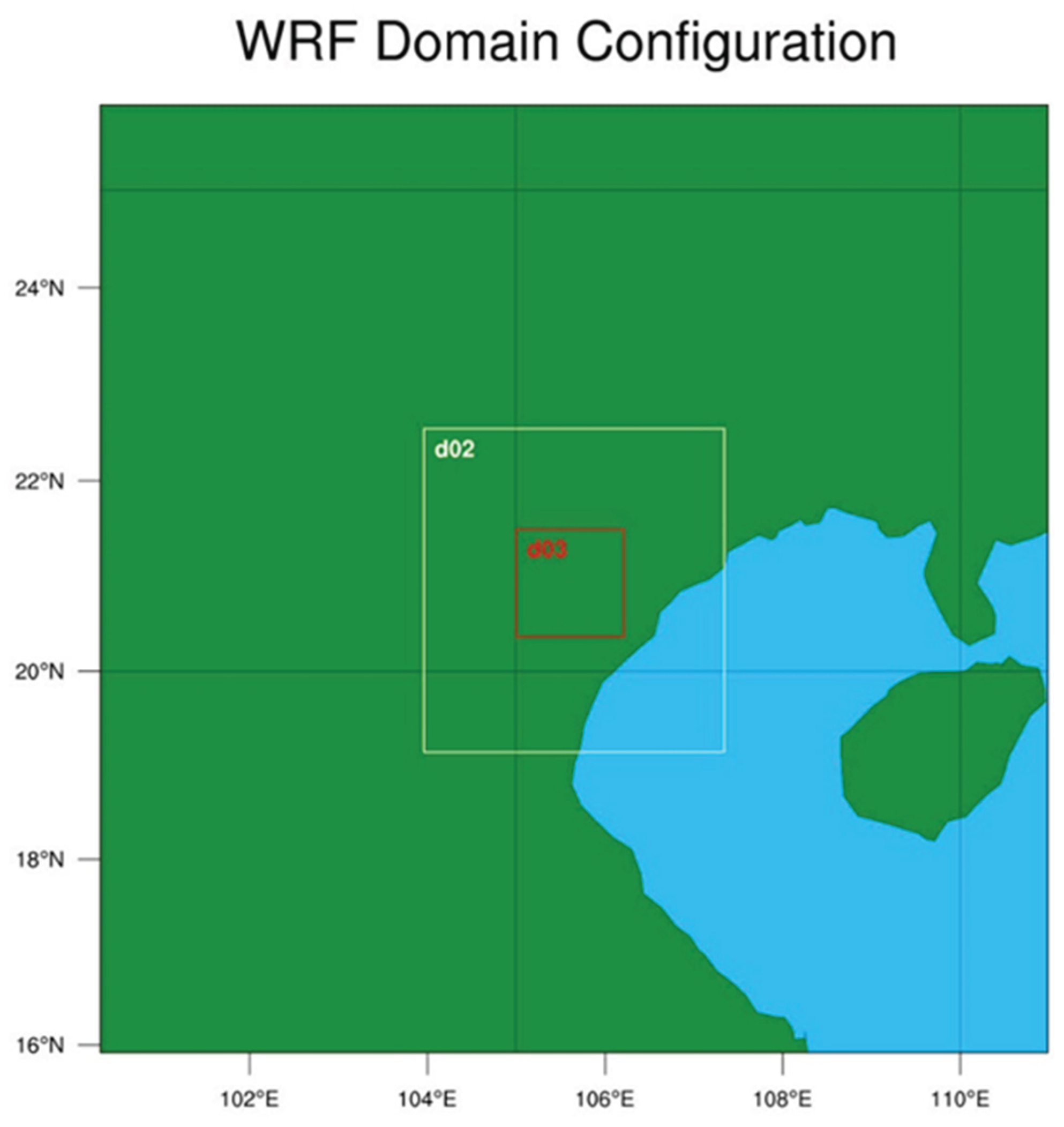
Figure 2.
Percentage contribution of pollutant sources in Hanoi (2022).
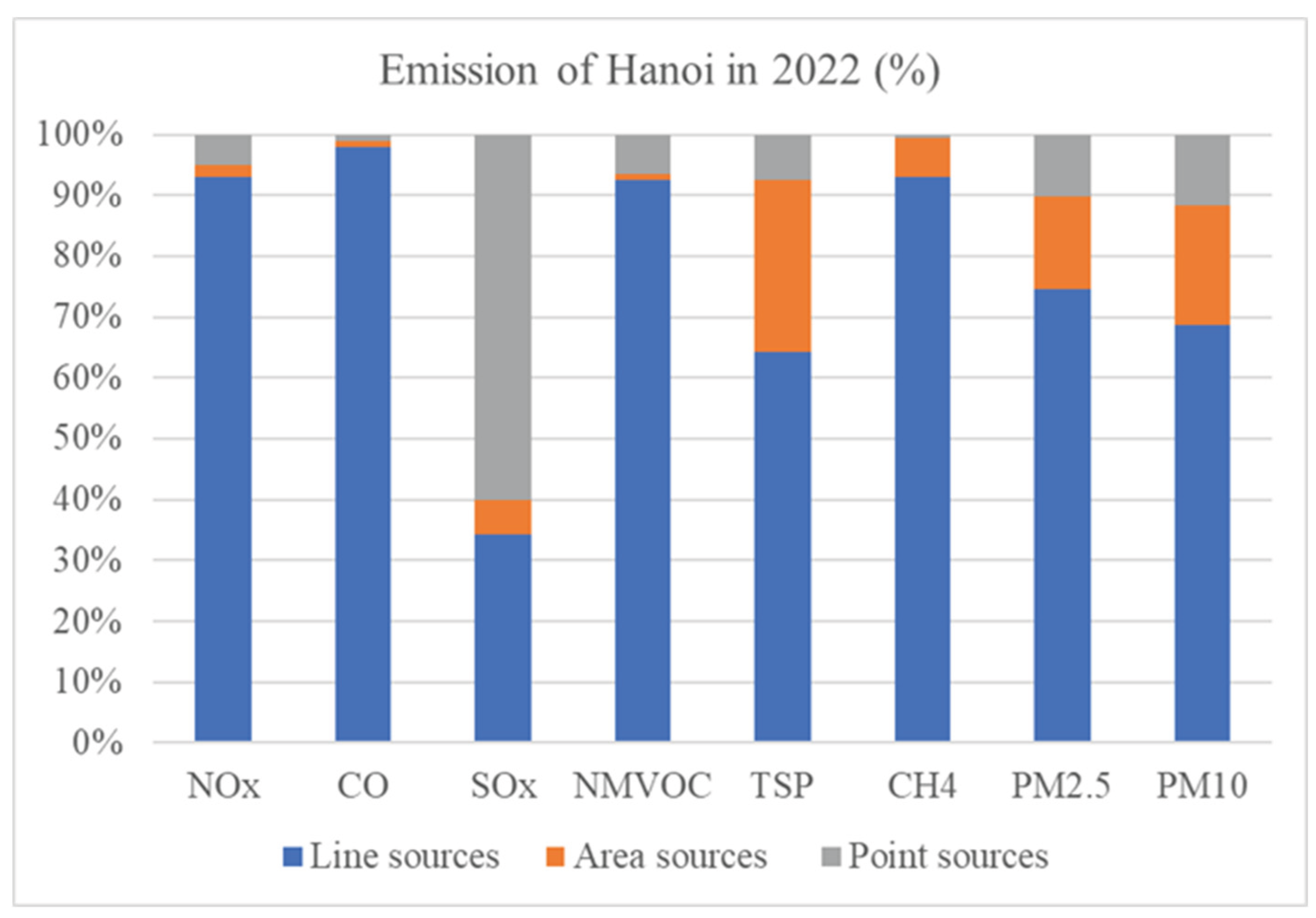
Figure 3.
Wind Rose Diagram at Ha Dong (January 2022) from results: (OBS) Observations, (WRF) Simulations.
Figure 3.
Wind Rose Diagram at Ha Dong (January 2022) from results: (OBS) Observations, (WRF) Simulations.
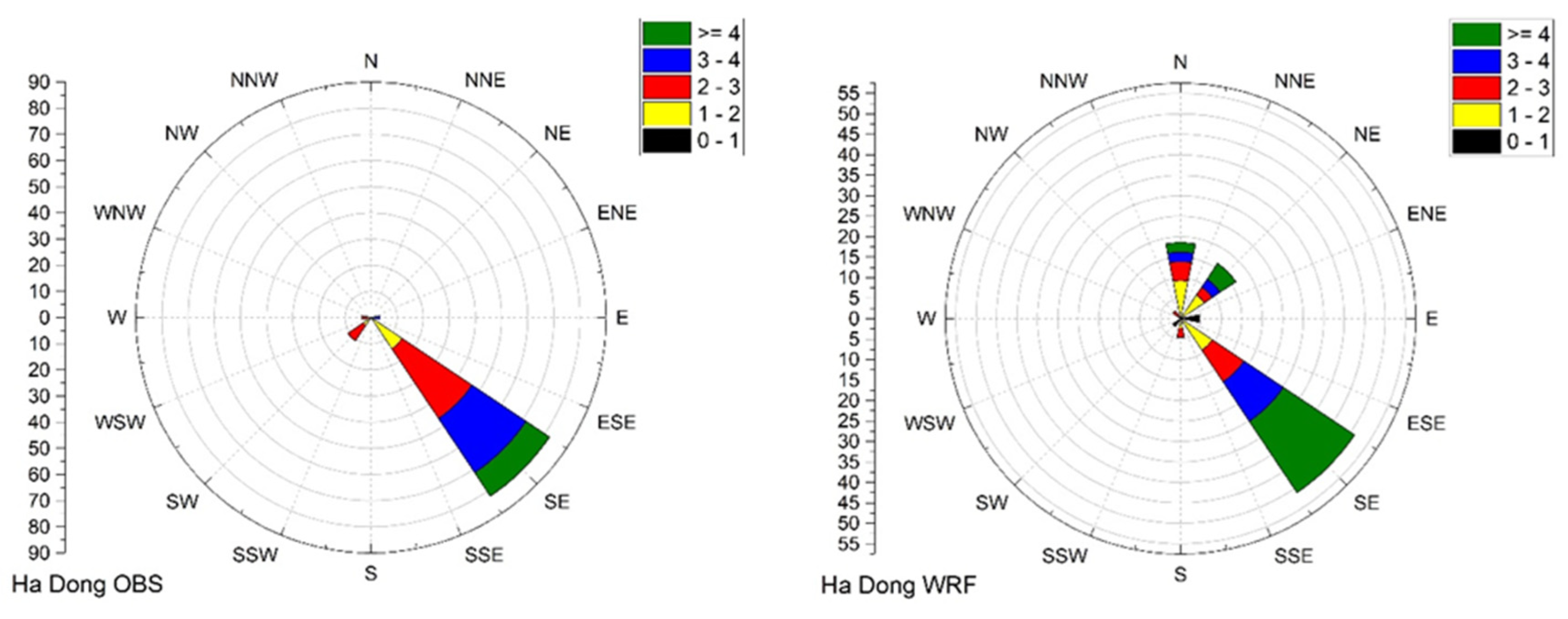
Figure 4.
The correlation coefficient between simulated and observed temperature at the U.S. Embassy station from January 15 to 18, 2022.
Figure 4.
The correlation coefficient between simulated and observed temperature at the U.S. Embassy station from January 15 to 18, 2022.
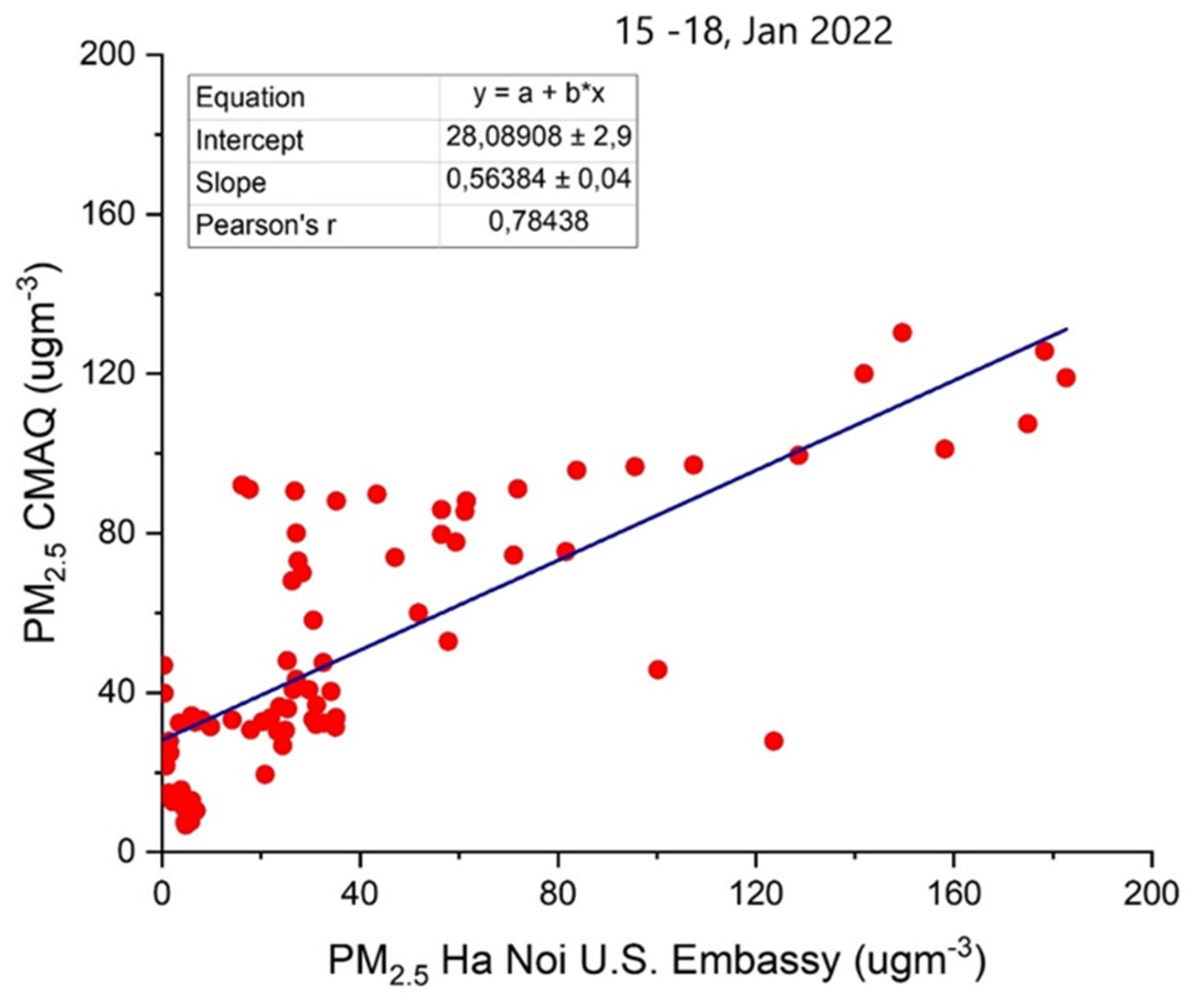
Figure 5.
Map of the average PM2.5 concentration distribution for (a) Jan, (b) July 2022 in the study area, CMAQ simulation results.
Figure 5.
Map of the average PM2.5 concentration distribution for (a) Jan, (b) July 2022 in the study area, CMAQ simulation results.
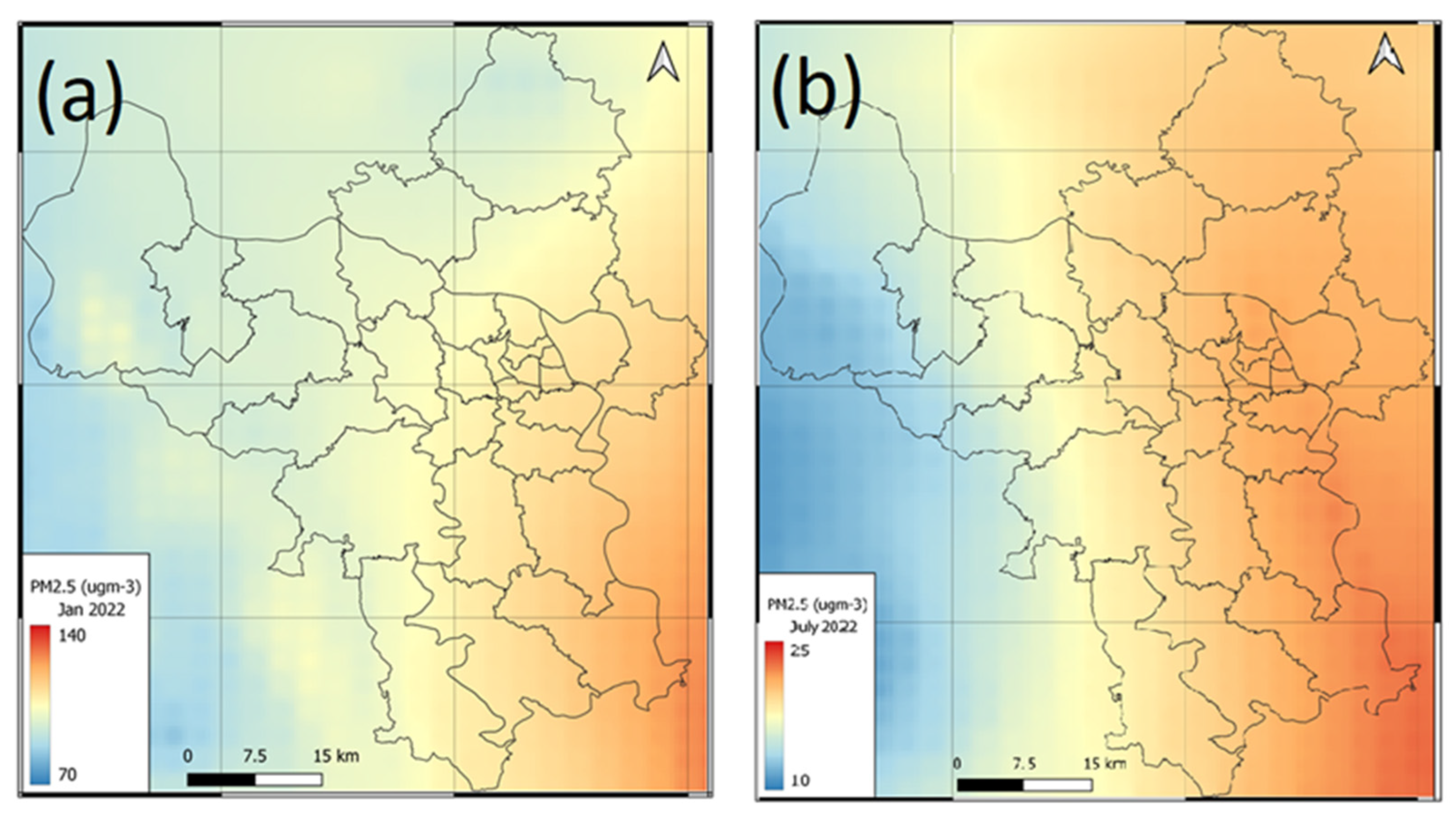
Figure 6.
Map of the average CO concentration distribution for (a) Jan, (b) July 2022 in the study area, CMAQ simulation results.
Figure 6.
Map of the average CO concentration distribution for (a) Jan, (b) July 2022 in the study area, CMAQ simulation results.
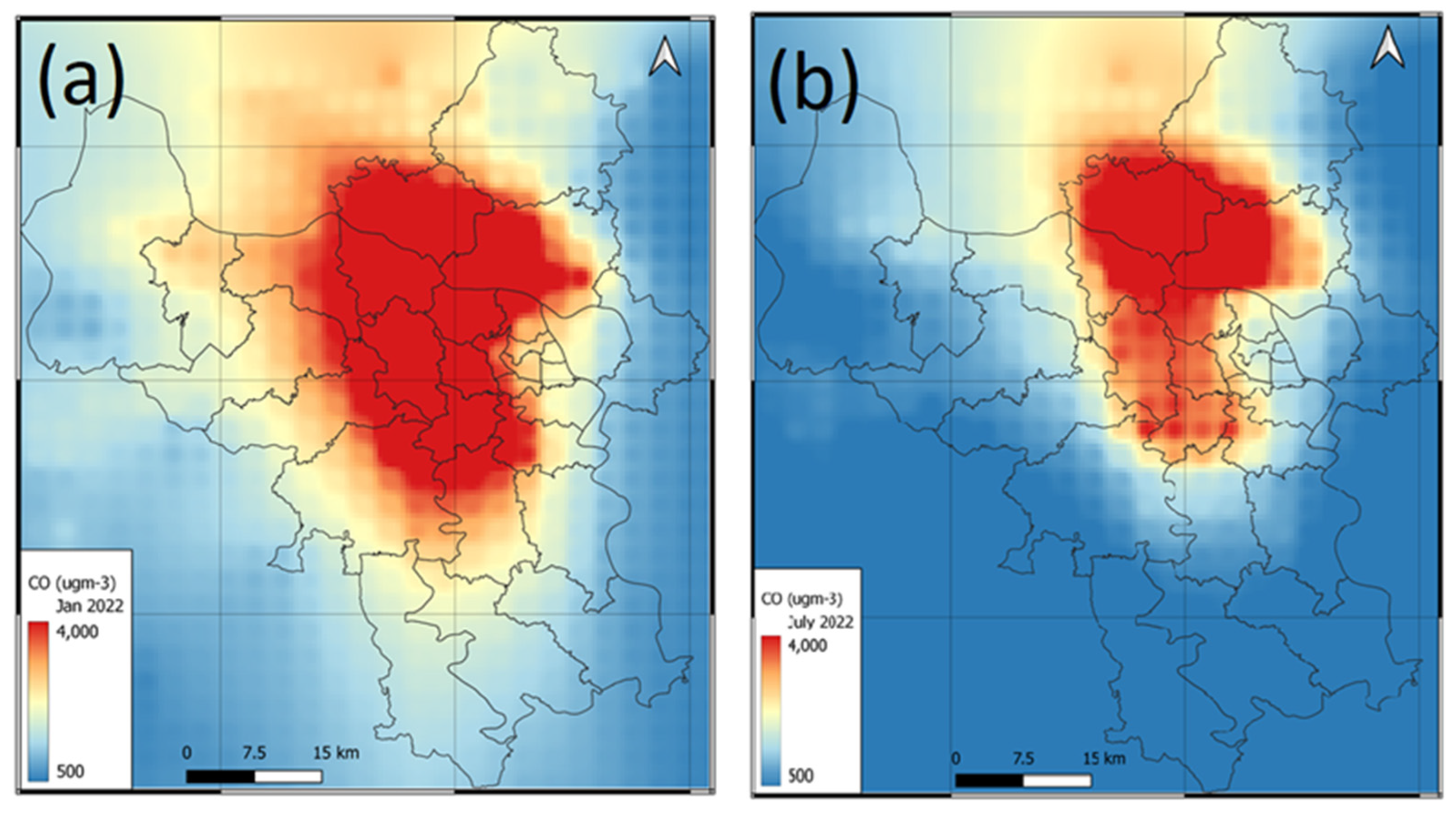
Figure 7.
Map of the average NO2 concentration distribution for (a) Jan, (b) July 2022 in the study area, CMAQ simulation results.
Figure 7.
Map of the average NO2 concentration distribution for (a) Jan, (b) July 2022 in the study area, CMAQ simulation results.
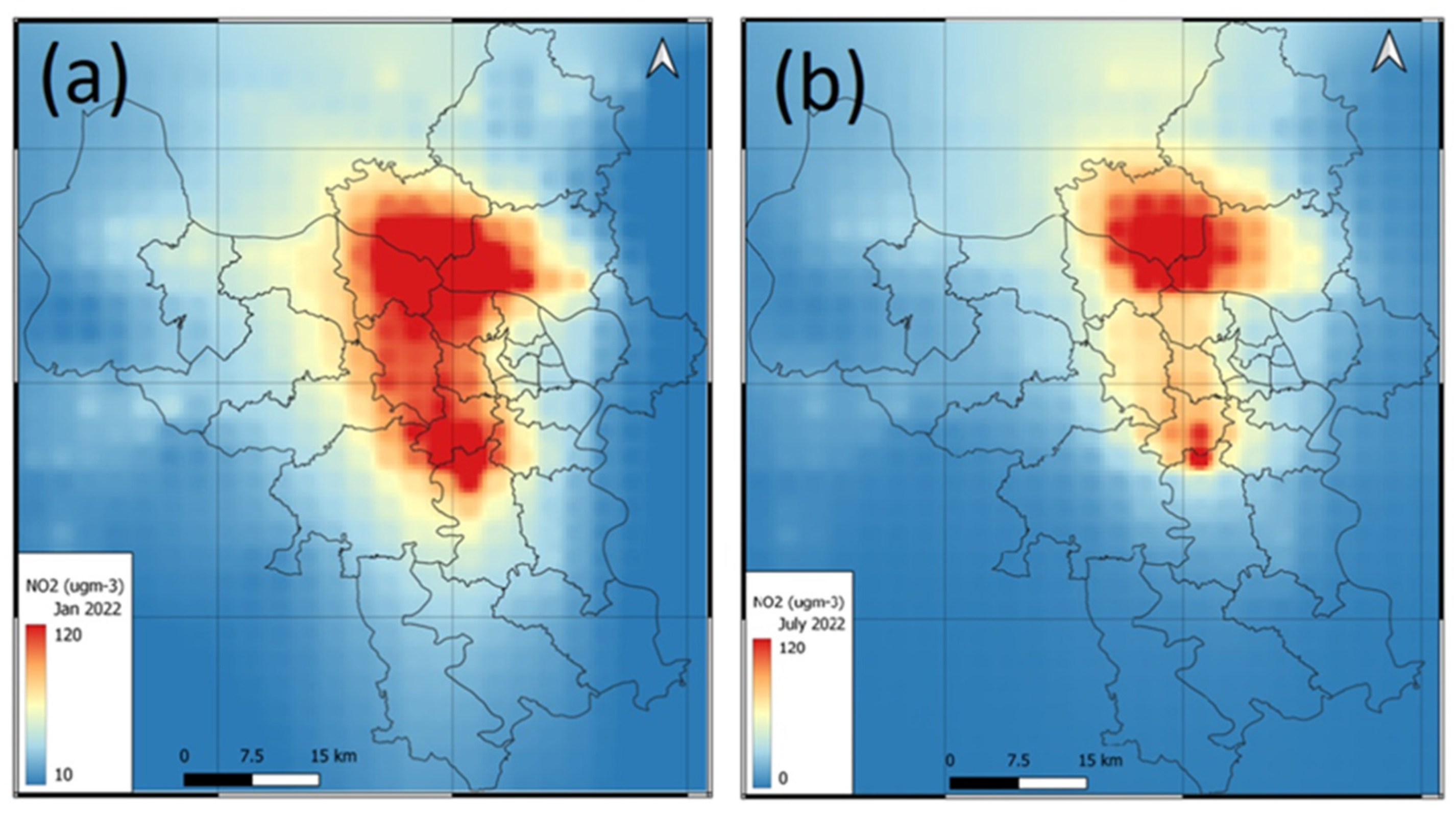
Figure 8.
Map of the average SO2 concentration distribution for (a) Jan, (b) July 2022 in the study area, CMAQ simulation results.
Figure 8.
Map of the average SO2 concentration distribution for (a) Jan, (b) July 2022 in the study area, CMAQ simulation results.
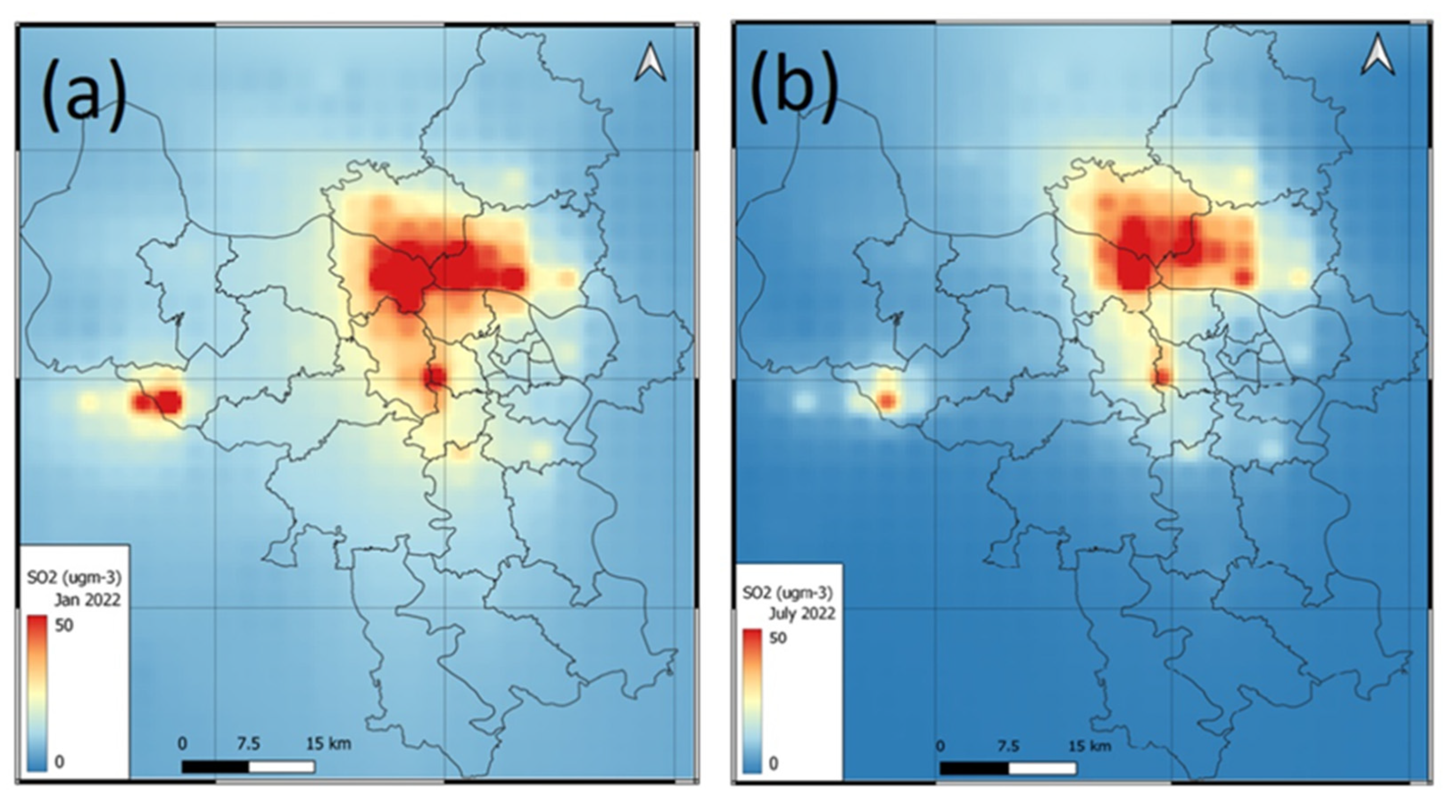
Figure 9.
Map of the average O3 concentration distribution for (a) Jan, (b) July 2022 in the study area, CMAQ simulation results.
Figure 9.
Map of the average O3 concentration distribution for (a) Jan, (b) July 2022 in the study area, CMAQ simulation results.
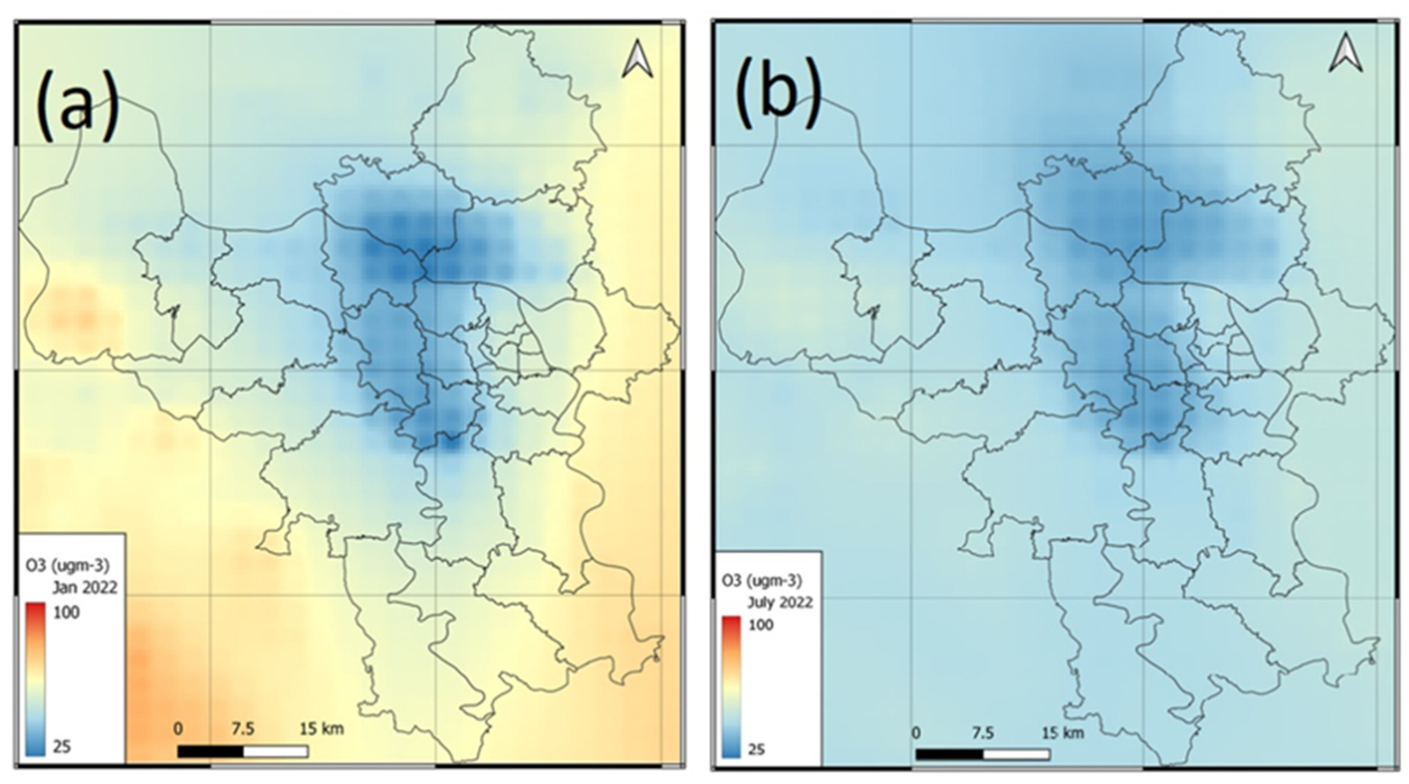
Figure 11.
Map of NO2 Concentration Difference Ratio between two scenarios for (a) January, (b) July across Domain 3.
Figure 11.
Map of NO2 Concentration Difference Ratio between two scenarios for (a) January, (b) July across Domain 3.
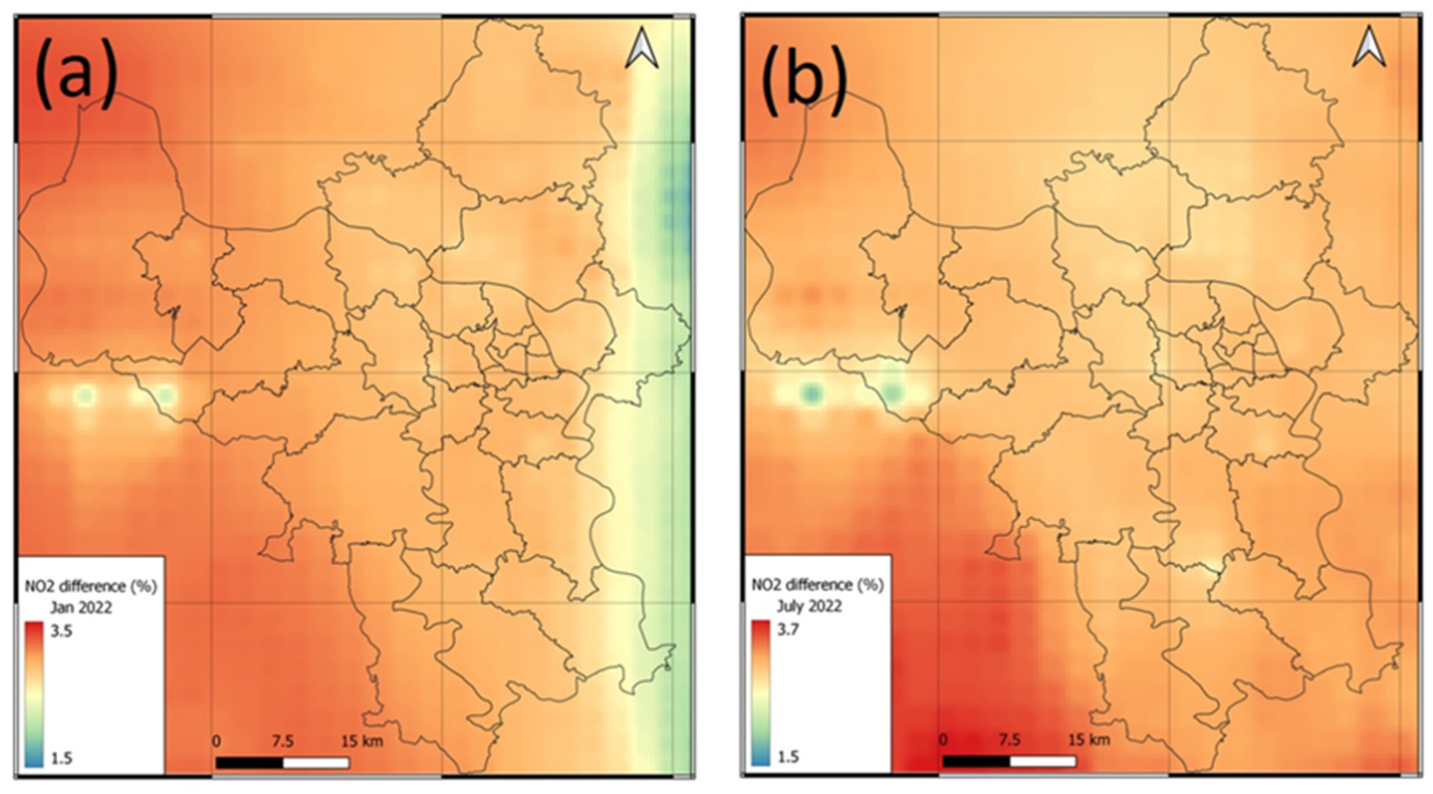
Figure 12.
Map of SO2 Concentration Difference Ratio between two scenarios for (a) January, (b) July across Domain 3.
Figure 12.
Map of SO2 Concentration Difference Ratio between two scenarios for (a) January, (b) July across Domain 3.
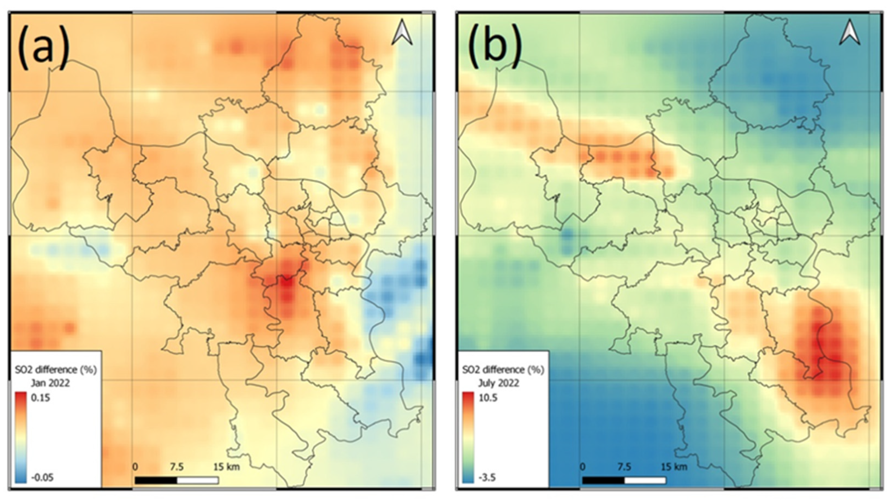
Figure 13.
Map of CO Concentration Difference Ratio between two scenarios for (a) January, (b) July across Domain 3.
Figure 13.
Map of CO Concentration Difference Ratio between two scenarios for (a) January, (b) July across Domain 3.
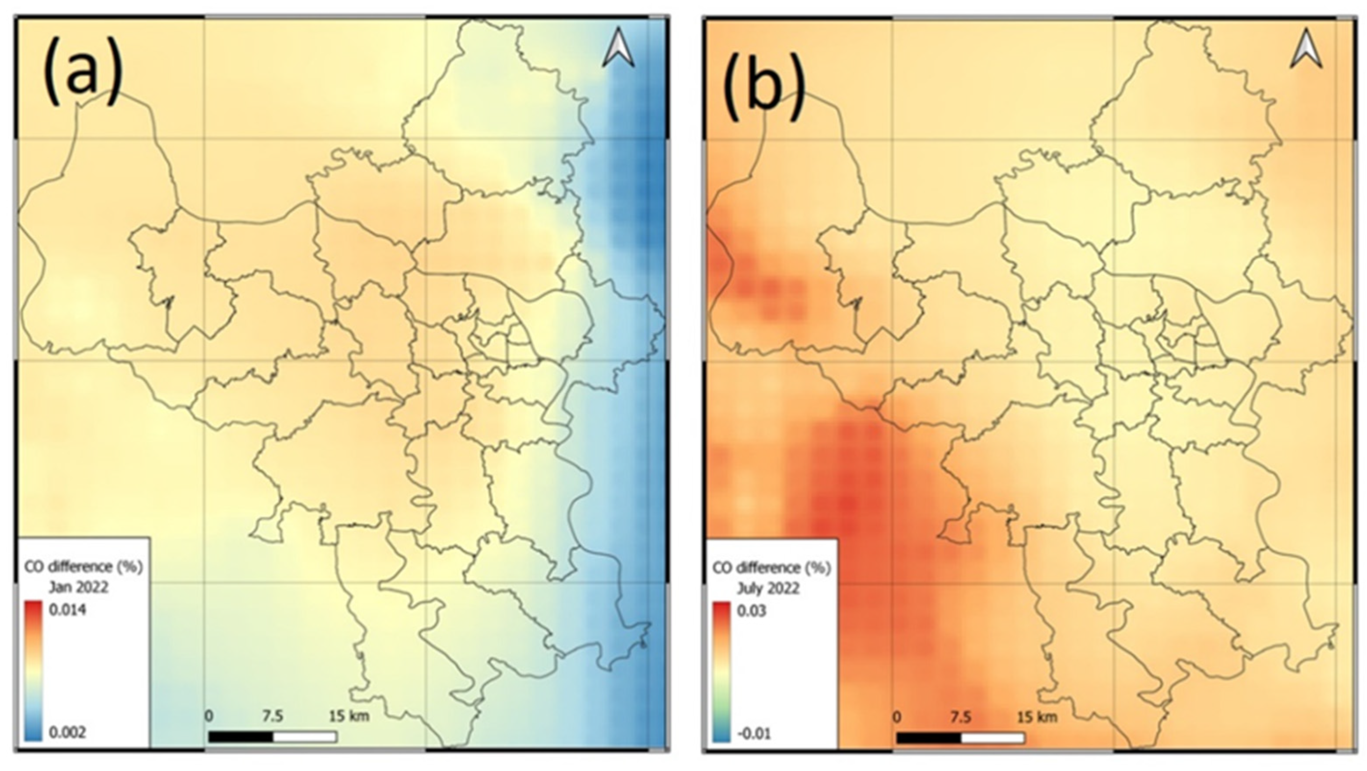
Figure 14.
Map of O3 Concentration Difference Ratio between two scenarios for (a) January, (b) July across Domain 3.
Figure 14.
Map of O3 Concentration Difference Ratio between two scenarios for (a) January, (b) July across Domain 3.
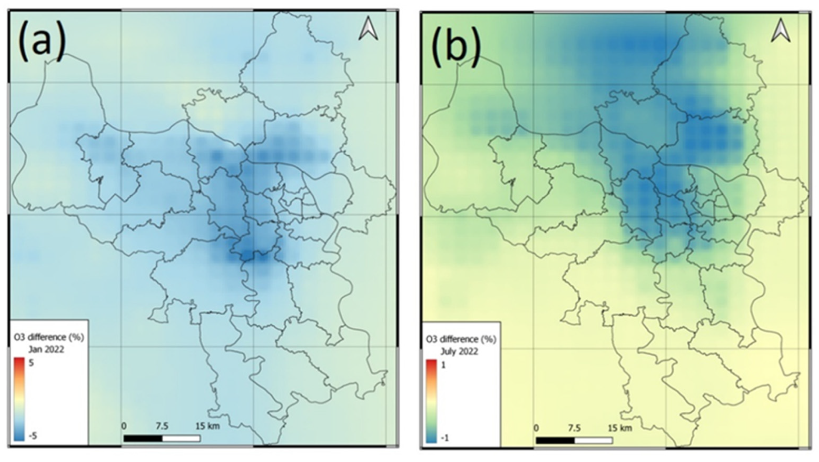
Figure 15.
Simulated PM2.5 concentration in January 2022, population distribution, population exposure and attributable deaths over the modelling domain. The high concentration of PM2.5 and population are concentrated in the Hanoi Old Quarter where the 3 monitoring stations (Minh Khai, Ba Dinh and Trung Yen) are located (marked as •). The old province of Hatay is now part of Hanoi city.
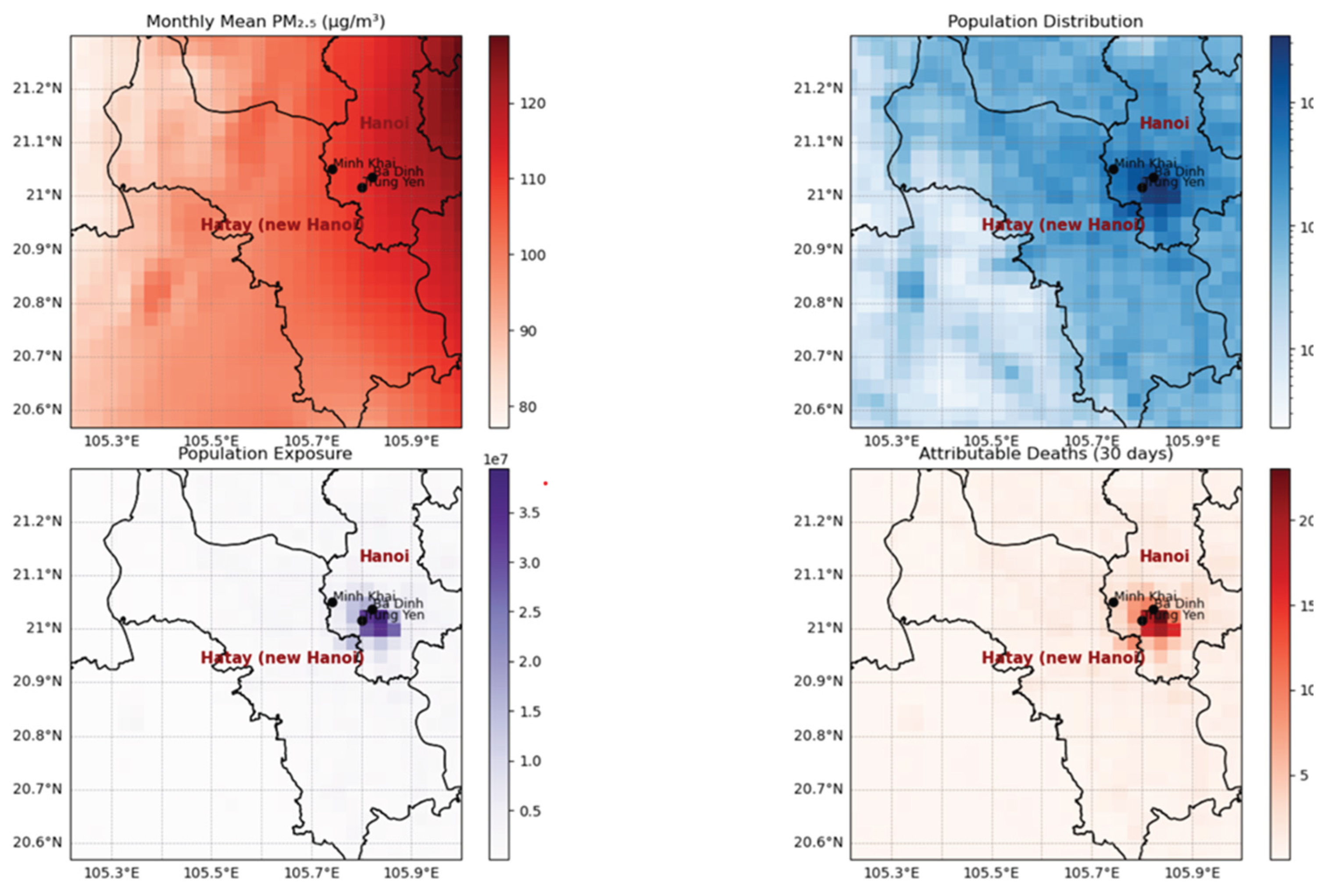

Table 1.
Model Setup and Physical Parameterization Used for WRF Simulation.
|
Table 2.
Emission of Hanoi in 2022 (ton/year).
| NOx | CO | SOx | NMVOC | TSP | CH4 | PM2.5 | PM10 | |
| Line sources | 69,907 | 2,033,569 | 4,025 | 189,225 | 33,271 | 30,826 | 29,757 | 31,388 |
| Area sources (including biomass burning) | 1,560 | 21,639 | 672 | 2,266 | 14,581 | 2,178 | 6,100 | 8,995 |
| Point sources | 3,788 | 21,351 | 7,038 | 13,195 | 3,859 | 165 | 4,044 | 5,312 |
| Total | 75,255 | 2,076,559 | 11,735 | 204,686 | 51,711 | 33,169 | 39,901 | 45,695 |
Table 3.
Emission Results of Pollutants from Bus Sources in 2022 for two Scenarios. (Unit: Tons/year).
Table 3.
Emission Results of Pollutants from Bus Sources in 2022 for two Scenarios. (Unit: Tons/year).
| Pollutant | Emissions from buses in Scenario 1 | Emissions from buses in Scenario 2 | Emission Reduction | Reduction Rate (%) |
| NOx | 14,613.3 | 12,365.7 | 2,247.6 | 15.38 |
| CO | 1,154.2 | 954.9 | 199.3 | 17.27 |
| SO2 | 58.8 | 50.6 | 8.2 | 14.02 |
| VOC | 347.8 | 290.7 | 57.0 | 16.40 |
| CH4 | 83.4 | 71.4 | 12.0 | 14.43 |
| NMVOC | 267.1 | 222.1 | 45.0 | 16.85 |
| PM2.5 | 4,727.5 | 4,192.3 | 535.3 | 11.32 |
Table 4.
Emission Results of Pollutants from Traffic Sources in 2022 for Two Scenarios (Unit: Tons/year).
Table 4.
Emission Results of Pollutants from Traffic Sources in 2022 for Two Scenarios (Unit: Tons/year).
| Pollutant | Emissions from traffic sources in 2022 | ||||
| Scenario 1 | Scenario 2 | Reduction Rate (%) | |||
| NOx | 69,907.4 | 67,600.2 | 3.30 | ||
| CO | 2,033,569.2 | 2,033,365.1 | 0.01 | ||
| SO2 | 4,025.0 | 4,016.5 | 0.21 | ||
| VOC | 150,081.8 | 150,023.3 | 0.04 | ||
| CH4 | 30,825.6 | 30,813.2 | 0.04 | ||
| NMVOC | 189,224.8 | 189,178.7 | 0.02 | ||
| PM2.5 | 29,756.8 | 29,202.2 | 1.86 | ||
Table 5.
The valuation parameters comparing the temperature and wind speed results from the WRF simulation with the observed data at Ha Dong meteorological station.
Table 5.
The valuation parameters comparing the temperature and wind speed results from the WRF simulation with the observed data at Ha Dong meteorological station.
| Index | Temperature | Wind speed | Reference Value |
| MAGE | 1.18 | 0.61 | ≤ 2 |
| RMSE | 1.38 | 0.70 | - |
| Factor 2 | 0.96 | 1.21 | 1.00 |
| R | 0.89 | 0.59 | - |
Table 6.
Monthly average of Air Pollutants in 2022 for Domain 3 (Unit: µg/m³).
| Air Pollutant | Jan | July | |||||||
| Average | Min | Max | Average | Min | Max | ||||
| PM2.5 | 100.1 | 77.3 | 128.9 | 17.0 | 9.3 | 23.2 | |||
| CO | 1861.8 | 505.3 | 11766.6 | 965.3 | 108.6 | 8583.4 | |||
| NO2 | 30.3 | 3.5 | 222.2 | 16.9 | 0.2 | 162.5 | |||
| O3 | 59.2 | 25.0 | 82.2 | 45.5 | 30.7 | 52.3 | |||
| SO2 | 11.8 | 5.4 | 104.9 | 5.2 | 0.3 | 85.0 | |||
* Min, max values across the entire domain D3.
Table 7.
Difference ratio of average Air Pollutant concentrations for January and July between the two scenarios for domain 3.
Table 7.
Difference ratio of average Air Pollutant concentrations for January and July between the two scenarios for domain 3.
| Air Pollutant | Jan | July | |||||
| Average | Min | Max | Average | Min | Max | ||
| PM2.5 | 0.017 | -0.064 | 0.088 | 0.3387 | -5.2564 | 5.1372 | |
| CO | 0.007 | 0.002 | 0.010 | 0.0166 | 0.0107 | 0.0298 | |
| NO2 | 2.964 | 1.592 | 3.420 | 3.1496 | 1.9106 | 3.7838 | |
| O3 | -1.959 | -5.558 | -0.831 | -0.2714 | -1.0228 | 0.0658 | |
| SO2 | 0.068 | -0.075 | 0.158 | 0.7998 | -3.5126 | 10.3743 | |
* Min, max values across the entire domain D3.
Table 7.
Mortality and cvd hospitalisation number with 95% confidence interval due to population exposure to PM2.5 air pollution in Hanoi. The PM2.5 ambient concentration is simulated using WRF-CMAQ air quality model. (*) The WHO PM2.5 safe guideline of 5µg/m3 is used as the reference concentration value below which there is no effect on health.
| January (dry season) | July (wet season) | |||
| Mortality | CVD hospitalization | Mortality | CVD hospitalization | |
| Overall baseline impact due to PM2.5 pollution (*) | 626 [245, 963] | 124 [-1, 232] | 94 [35, 152] | 18 [0,36] |
| Overall impact due to PM2.5 pollution with 50% EV buses in fleet (*) | 625 [245, 962] | 124 [-1, 232] | 94 [35, 152] | 18 [0,36] |
| Change in impact between baseline and 50% EV buses scenarios. | 0.25 [-717, 717) | 0.05 [-233, 234] | 0 [-117, 117] | 0 [-36, 36] |
Disclaimer/Publisher’s Note: The statements, opinions and data contained in all publications are solely those of the individual author(s) and contributor(s) and not of MDPI and/or the editor(s). MDPI and/or the editor(s) disclaim responsibility for any injury to people or property resulting from any ideas, methods, instructions or products referred to in the content. |
© 2025 by the authors. Licensee MDPI, Basel, Switzerland. This article is an open access article distributed under the terms and conditions of the Creative Commons Attribution (CC BY) license (http://creativecommons.org/licenses/by/4.0/).
Copyright: This open access article is published under a Creative Commons CC BY 4.0 license, which permit the free download, distribution, and reuse, provided that the author and preprint are cited in any reuse.


