Submitted:
16 October 2025
Posted:
17 October 2025
You are already at the latest version
Abstract
This study explores the mechanisms through which the street built environment(BE) influences mobile physical activity (MPA) using multi-source data and explainable machine learning methods. The research combines Geographically Weighted Regression (GWR) and Random Forest (RF) models to reveal the complex spatial heterogeneity between BE factors and MPA, and enhances the interpretability of results through the SHAP model, providing theoretical support for future targeted urban planning and MPA interventions. The study finds that the "density" dimension of BE plays a crucial role in MPA, particularly population density and building density. Additionally, accessibility and safety also significantly influence MPA, while design factors such as greening rates, water landscapes, and building façade design promote MPA. The study emphasizes that the influence of BE factors on MPA is nonlinear, with significant interaction effects between different variables, indicating that improving a single variable alone cannot fully explain changes in MPA. This research provides a new theoretical perspective for understanding the impact of BE factors on MPA and offers empirical evidence for precise interventions. In areas with low MPA participation, improving street design, enhancing traffic safety, and increasing green and water-friendly spaces can significantly promote residents' MPA, thereby improving public health.
Keywords:
built environment
; mobile physical activity
; perceptual perspective
; machine learning
; nonlinear effects
; interactive effects
; urban planning
1. Introduction
Since the 21st century, the global health landscape has been undergoing profound changes, with chronic non-communicable diseases becoming the primary threat to human physical and mental health [1]. Physical activity(PA) is widely regarded as the cornerstone of maintaining and promoting health [2]. Regular PA can reduce the risk of chronic diseases and offers numerous benefits for maintaining both physical and mental health. Among various types of PA, mobile physical activities(MPA) such as running and cycling have become key targets for promoting public PA. This is due to their low infrastructure investment and exercise implementation costs, and numerous studies have shown that optimizing the built environment(BE) can significantly enhance the public’s behavioral adherence to MPA [3,4,5,6,7].
Given the effective promotion of MPA by the BE, many scholars have conducted studies on the relationship between BE factors and MPA to develop scientifically effective MPA intervention measures. Previous work on the measurement of BE factors mainly focused on the classic "5Ds" model [8], which includes factors such as the accessibility of service facilities [9,10], population density [11,12,13], intersection density [14,15], landscape features [16,17,18], and visual quality [4,5,19]. Existing research indicates that BE impacts MPA mainly in three aspects: First, BE factors such as road intersections, traffic lights, and road network density significantly affect the frequency of MPA. These traffic organizations disrupt the continuity of MPA, thereby reducing its frequency and environmental attractiveness. Second, the neighborhood environment reflecting greening levels is closely linked to MPA, including green spaces, green coverage, and water-friendly spaces. Third, BE also influences MPA in terms of functionality, with mixed land use, residential density, and open space density showing certain correlations with MPA. It should be noted that regarding mixed land use, some studies have shown its significant effect on commuting-related MPA, but the effectiveness of its impact on recreational MPA remains uncertain [6].
In existing studies, although many scholars have explored the impact of different BE variables on MPA, most of these studies focus on objective environmental measurements and lack a systematic consideration of human perception. In reality, human behavior is not determined solely by the physical environment—perception plays a crucial role [19]. An individual’s perception of the environment influences their behavior choices. For example, certain streets in urban areas may be more likely to attract people to walk or cycle due to greenery, a sense of openness, or perceived safety. These perceptual factors often have a more direct impact on MPA behaviors than objective spatial structural factors. Therefore, from a perceptual perspective, exploring the mediating role of perception in behavior can help reveal the complex relationship between the BE and MPA, fill gaps in existing research, and provide theoretical support for the development of precise intervention strategies.
On the other hand, the impact of BE on MPA is spatially heterogeneous [20], meaning that the influence of BE on residents’ MAP may vary significantly across different geographic regions. Existing statistical methods often assume that the influence of BE on MPA is homogeneous across space, a hypothesis that overlooks the differences in BE characteristics and residents’ MAP behaviors in different areas [5,6,14,21]. Therefore, it is crucial to adopt analytical methods that account for spatial heterogeneity [20]. This study employs a hybrid model that combines Geographically Weighted Regression (GWR) and Random Forest (RF), incorporating spatial weight matrices and machine learning algorithms to effectively handle spatial heterogeneity and non-linear effects. The GWR model assigns different weights to each sample based on geographic location, capturing the variations in local environmental factors; while the RF model efficiently handles complex non-linear relationships, helping to uncover the hidden patterns between BE and MPA. By combining spatial heterogeneity analysis and machine learning methods, we can more accurately reveal the mechanisms through which BE influences MPA.
The innovations of this study are mainly reflected in the following aspects: First, it uses micro-scale street-level data combined with a perceptual perspective to analyze how individuals’ perceptions of the street BE influence their MPA behavior. Second, it introduces spatial heterogeneity and nonlinear analysis methods, enhancing the model’s ability to capture the complex relationship between BE and MPA. Finally, by incorporating the SHAP model, the study provides a clearer framework for the interpretability of the results, further increasing the practical and policy guidance value of the research.
By combining the perception perspective with spatial heterogeneity machine learning methods, the research framework proposed in this study provides greater explanatory power for street-level MPA research. This framework not only reveals the impact mechanisms of various factors in the BE but also provides data support for urban planners and policymakers to implement targeted interventions. Ultimately, this research offers new theoretical foundations and practical pathways for the construction of healthy cities and the promotion of MPA.
2. Materials and Methods
2.1. Framework
The technical framework and workflow of this study are shown in Figure 1. It mainly consists of the following three parts:
(1) Data processing and variable calculation, which includes improving the traditional "5Ds" built environment indicator system from a perceptual perspective to form the built environment variable set used in this study;
(2) Model training and result interpretation, which involves the construction and interpretation of the GW-RF machine learning regression model, balancing the "perception-behavior" logical framework with the "spatial heterogeneity processing ability";
(3) Result analysis, which includes variable importance, direction of effects, nonlinear effects, variable interactions, and spatial interpretation of the effects of some variables.
2.2. Study Area
Chengdu is located in Sichuan Province, China, and has a subtropical monsoon climate with an average annual temperature of 16°C, making the climate pleasant. The region has a flat terrain, crisscrossing river networks, and beautiful scenery, and is known as the "City of Leisure". As the capital of Sichuan Province and a core city in the Chengdu-Chongqing Twin-City Economic Circle, Chengdu has a permanent population of 21.192 million. The roads in the main urban area extend radially from the center to the surrounding areas, with flat roads and numerous sidewalks. Chengdu’s superior natural conditions such as climate and terrain, along with the guidance of leisure and fitness culture, have created a favorable environment for residents in this region to engage in outdoor MPA [22].
This study takes the main urban area of Chengdu as the research object, covering Jinniu District, Qingyang District, Jinjiang District, Wuhou District and Chenghua District. As the core area of Chengdu’s population and economy, the main urban area is not only the political, cultural and commercial center of Chengdu, but also the main place where residents engage in PA. Although the research scope of this study is the main urban area, considering that the public do not take administrative boundaries as rigid activity boundaries when engaging in PA, this chapter finally selects the area formed by expanding a 1500m buffer zone outward based on the boundary of Chengdu’s main urban area as the research area, and the scope is shown in Figure 2.
2.3. Datasets
2.3.1. PA Data
Users’ PA data is recorded by the Keep App1 and does not involve personal privacy. Keep App, along with Codoon App and Yuepaoquan App, is one of the three most popular outdoor fitness tracking apps in China, boasting a large user base. The popular routes on Keep are spontaneously uploaded by users to share high-quality routes in urban spaces that they consider safe and open to the public. They represent a collection of spatial locations in the city, filtered by users, which are suitable for MPAs such as running, walking, and cycling [7].The popular routes on KeepApp include the following information: route name, route ID, route location, venue type, route length, check-in count, proportion of PA types, route creation date and route shape (see Table 1 for detailed data structure). The study area includes a total of 631 popular routes, of which 212 are street routes. After manual verification and excluding non-street routes mistakenly labeled by users, 200 popular routes were selected as the foundational data for this study.
This study completed the vectorization of popular routes using the ArcGIS platform. First, the geographic coordinates of the routes were used to determine their spatial location. Next, the vectorization of the routes was manually completed within the study area’s single street network. For each street (segment) passed by a popular route N times, the "Route-Count" attribute in the street’s attribute table is recorded as N, ensuring that the PA indicators of streets passed by multiple routes or multiple times by a single route are accurately recorded and reasonably calculated. The vectorization results are shown in Figure 3.
Given that the basic unit of study is the "street," specifically referring to the segments in the single-line network vector map formed by processing the study area’s road network into a single centerline, the 200 popular routes are marked onto the study area’s single-line network vector map. This involves 2,019 street segments, with the longest segment measuring 1,364.27 meters, the shortest measuring 18.71 meters, the average length being 202.94 meters, and a standard deviation of 154.15 meters. A summary of the vectorized data for the popular routes within the study area is shown in Figure 4(a).
Since the GW-RF model in the later sections requires the processing of spatial coordinate data for each sample, and "street segments" as linear vector features, are difficult to directly incorporate into the calculation, they need to be abstracted as individual "points" in space, with the "point coordinates" then used as input for the model. Therefore, based on the ArcGIS platform, this study uses the "Feature to Point" tool to convert the line vector features of each street segment into point vector features. It should be noted that in the ArcGIS platform, when converting line features to point features, the resulting points are not necessarily the "midpoints" of the line features. For linear line features, the generated point feature is located at the midpoint of the line segment; however, for polyline or curve line features, the resulting point is located at the weighted average of the x and y coordinates of all the segment midpoints. Specifically, assuming a polyline consists of n segments, the coordinates of the midpoint for each segment are weighted (with the weight being the length of each segment) and averaged to obtain the coordinates of the generated "point feature." The spatial relationship after converting the polyline is shown in Figure 4(b).
2.3.2. Multi-Source Urban Data
The multi-source urban data used in this study includes road network data, water body data, population raster data, street view image data, point of interest data, and building footprint data.
The road network data is sourced from OpenStreetMap. After single centerline processing and manual verification, a total of 25,224 street(segment) samples were obtained. Water body data also comes from OpenStreetMap, including both linear and polygonal water body data. After manual verification, the polygonal water body data covers wider river sections of Fu River, Nan River, Jinjiang, Jiang’an River, Sha River, and Dongfeng Canal that flow through the study area, as well as natural and artificial lakes within the study area. The linear water body data primarily covers the narrower rivers and canals in the remaining parts of the study area. Population raster data is sourced from the WorldPop open data platform. Street view image data is from the Baidu Map. Based on the ArcGIS platform, this study generated a total of 51,127 street view sampling points with 50m intervals using the study area’s single-line network vector map as the base. For road segments shorter than 50m, the midpoint was used as the sampling point. Through the Baidu Street View API, a total of 43,271 unique street view images were collected. Building data is sourced from the Baidu Map. By calling the Baidu Map API and comparing it with manually sampled satellite imagery, a total of 133,239 individual building vector data (including building footprints and number of floors) within the study area was obtained. The POI data is from the Amap. By calling the Amap API and filtering within a 50m buffer zone on both sides of the street using the ArcGIS platform, a total of 196,291 POI points were identified. The data sources and detailed descriptions are provided in Table 2.
2.4. Variables
2.4.1. Dependent Variables
Existing research has indicated that BE factors are the main determinants of the intensity of PA rather than its frequency [7]. Therefore, in this study, when extracting PA indicators, the per capita PA intensity is used as the outcome variable for the model, with the calculation logic as follows:
a. Based on the original data of each popular route, calculate the annual average check-ins W1.
Assuming that the cumulative check-ins for a certain popular route is W0, and the route has been active for N months until the data collection time (June 2024), the annual average check-ins can be calculated as W1.
b. Based on the annual average check-ins, calculate the annual PA intensity I0 for the street segments passed by the popular route.
Assuming that the popular route passes through street segment A, and the number of times it passes through segment A is n, with the length of segment A being L, the total annual PA intensity I0 for segment A can be calculated based on the annual average check-ins W1, along with the number of times segment A is passed (n) and its length (L).
c. Based on the total population near the street segment, calculate the annual per capita PA intensity I1 for the segment.
Considering the proximity characteristic of the public’s daily PAs, taking street segment A as the reference, a buffer zone with a 250m radius at the block scale is defined. Based on the population raster data, the total population P within the buffer zone surrounding the street is extracted, and then the annual per capita PA intensity (I1) for the segment is calculated.
In summary, the formula for calculating physical activity intensity is:
Finally, the descriptive statistical indicators of PA intensity for all street segment samples in this study are as follows: the number of sample segments is 2,019, with a maximum value of 1,698.04m, a minimum value of 0.04m, an average of 27.12m, and a standard deviation of 104.94m. The PA intensity indicator exhibits a distinct concentric distribution pattern, with a general "inner ring low, outer ring high" distribution around the Third Ring Road of Chengdu, as shown in Figure 5.
2.4.2. Environmental Variables
This study is based on the classic "5Ds" framework for describing BE indicators. On this foundation, on one hand, it takes public perception as the starting point and uses the "visually perceptible maximum scale" as the spatial scale basis for statistical indicators (psychologically, it is believed that the maximum distance for social interaction on streets is 100 meters [23,24]). The study selects BE elements that the public can directly or indirectly observe as environmental variables. On the other hand, considering the significant impact of safety perception on public behavior, the "Safety" dimension is added to the "5Ds" framework as a supplement. The definition and description of environmental indicators are detailed in Table 3, and the descriptive statistics of the indicators are shown in Table 4.
①Density
In the "5D model" framework, density refers to the concentration of population, buildings, or facilities within a unit area, reflecting the degree of resource concentration in urban space. Common indicators include population density, building density, and POI density. This study adopts the same 3 indicators, but with a difference in scale compared to previous research. For population density and building density, the street edge is taken as the baseline, and a bidirectional buffer zone is applied within a 100m range, which is the maximum scale of human visual perception. For POI density, only street-facing POIs are included in the statistics to calculate their density. The rationale behind this is that for individuals engaging in regular PA on the street (regular PA is defined as exercise for fitness purposes, rather than for leisure, entertainment, or commuting), the functional attributes provided by commercial facilities (POIs) along the street are not the main focus. Instead, the perception of such individuals is influenced by the decorative storefront designs, such as signs and windows, and the customer flow entering and exiting the stores. Therefore, non-street-facing POIs should have no perceptible effect on this group.
②Diversity
The diversity in the built environment reflects the degree of mixing of different functional spaces within a region, aiming to demonstrate the balance and complexity of regional functions. Land use function mix and POI diversity are commonly used to measure the diversity of facilities. Land use function mix is typically calculated by computing the area proportion of different land use types within a plot to determine the entropy value. On one hand, this approach is more suitable for research scenarios at the scale of blocks or administrative units. On the other hand, since land use data is usually based on land use planning maps, there is often a certain discrepancy between the data and the actual situation.
POI data, as a point-based dataset, although it cannot fully reflect the size differences between facilities (e.g., a convenience store and a large supermarket are both categorized as commercial facilities but offer significantly different shopping opportunities and attractions), it is open-source and, on one hand, facilitates research across different spatial scales based on precise geographic coordinates. On the other hand, POI data can accurately mark the physical locations of facilities serving different functions, such as commercial, residential, and public services, allowing for the measurement of the density and diversity of different functional facilities.
Therefore, this chapter ultimately chooses to use POI data that reflects different types of functional facilities (including living and education facilities, transportation facilities, and recreational and sports facilities) to calculate their density, reflecting the diversity of street functions. The spatial scale is consistent with the "density" section above, and only POIs along the streets are included in the calculation.
③Design
The design dimension of the built environment focuses on the physical characteristics of spatial form and street networks, involving aspects such as architectural design, street design, and public space design. Reasonable architectural design can improve space utilization and environmental comfort, street design affects traffic flow, pedestrian safety, and accessibility, and high-quality public space design can provide residents with good recreational venues, increase community cohesion, and enhance the quality of the built environment. Common design dimension indicators primarily include the following three aspects:
1. Street network structure: Including road intersection density, street network density, etc.
2. Environmental design: Such as building interface continuity, street width-to-height ratio, blue-green landscapes, etc.
3. Facility dimension: Including pedestrian facilities, accessibility facilities, etc.
In this study, at the street network structure level, since street network density is not an environmental indicator directly perceivable by the public, its representation of street network accessibility characteristics will be reflected in the subsequent "Accessibility Dimension" through corresponding indicators. At the environmental design level, this study uses building interface continuity to reflect the regularity of street-facing building facades, and selects the visual exposure of linear water bodies (such as small rivers, ditches, etc.) and polygonal water bodies (such as wide river surfaces and lakes) to reflect the perception of blue landscapes. Furthermore, through the analysis and extraction of street view image data, sky view factor is selected to reflect the openness of the street, and green view factor is chosen to reflect the perception of green landscapes in the street space. At the facility dimension level, the proportion of pedestrian walkways in the street space is extracted from street view images to reflect the distribution of walking facilities in the street environment.
④Distance to Transit
The convenience of the public transportation system measures the proximity between the built environment and public transportation facilities (such as subway stations, bus stops, etc.). The closer the public transportation is to residential areas, the more convenient it is for residents to use public transport, which helps reduce the use of private vehicles, alleviate traffic congestion, lower carbon emissions, and improve the accessibility and convenience of residents’ travel, thus expanding their range of activities. Based on previous research [4,5], this study ultimately selects the number of bus stops and metro stations along the street as indicators for calculation.
⑤Accessibility
Accessibility, as defined in the "5D" framework, refers to the "spatiotemporal convenience of reaching specific functional locations (such as parks, supermarkets, bus stops, etc.)." Its core focus is on the "functional value of the street as a path," which includes the physical distance from the current street to external destinations, functional compatibility, and psychological accessibility (such as the coverage of parks within a 500m buffer zone, or the network distance to a bus stop, etc.). This definition emphasizes the connection between streets and external places, essentially serving the analysis of "travel behavior from A to B." Existing studies have shown that the explanatory power of accessibility for commuting-related PAs is much higher than for recreational PAs [6,20]. This is partly because recreational PAs are inherently harder to predict compared to commuting activities, and partly because of the definition of accessibility itself. The "from A to B" travel behavior is different from recreational PAs aimed purely at exercise, and this difference is, to some extent, distinct from the definition of accessibility in the "5D" framework.
Since this study focuses on "MPAs aimed at exercise occurring on streets," it emphasizes whether streets can attract pedestrian flow for physical exercise, rather than the "convenience of traveling from the street to external places." Therefore, this study, referencing existing research [25,26,27], adopts the "global normalized angular accessibility (NAch_Global)" indicator from space syntax as a substitute variable to describe the accessibility of the street network. Existing studies have shown that the global NAch indicator effectively captures the overall structure of the street network. By quantifying the spatial connectivity depth in the network’s topological structure, it can effectively reflect the convenience of reaching a target location from any point in the network [28,29].
⑥Safety
Existing research has shown that safety perception is a commonly used indicator in studies of the built environment’s impact on PA [3,21,30]. Safety perception mainly refers to residents’ perceptions of neighborhood crime and road safety, with measurements typically including perceived safety of walking paths, crime rates, and traffic hazards. It can be said that safety perception is a fundamental influencing factor for PA and one of the basic needs for residents to engage in MPA on the streets. Among these factors, increased motor vehicle traffic significantly reduces residents’ willingness and frequency of walking, making it the primary factor influencing the perception of safety in PA.
Meanwhile, the NAch indicator has been proven to be scientifically effective in the quantitative analysis of vehicle flow in urban traffic networks. Several empirical studies have shown that the NAch indicator has a good fit with actual traffic data [25,31]. It is important to note that in the space syntax calculation process, the NAch indicator’s description of urban street network structural features and its predictive performance for traffic flow are closely related to its scale. An empirical study on ground traffic flow in Chongqing has shown that the local angular accessibility indicator at a specific scale fits actual traffic flow better than the global integration and global angular accessibility indicators [25].
Given the difficulty in obtaining real traffic flow data for validation, and considering the excellent ability of the machine learning models used in the subsequent regression analysis to handle complex multicollinearity factors. This study based on empirical parameters from previous research [25], incorporates the local NAch indicator (with a radius of 7km, NAch_7k) as a proxy for road motor vehicle flow into the set of indicators.
2.5. Methods
2.5.1. GW-RF Model
This study introduces a hybrid model based on Geographic Weighted Regression (GWR) and Random Forest (RF), called the "Geographic Weighted-Random Forest" (GW-RF) model, to explore and analyze the relationship between the built environment and PA. The GW-RF model combines the spatial heterogeneity modeling capability of GWR with the nonlinear processing ability of RF. In the GW-RF model, the GWR is used to handle local feature differences in the built environment at different geographic locations. It introduces a weighting coefficient spatially to process geographic location differences for each sample, ultimately generating a Spatial Weight Matrix (SWM) based on the spatial position of the samples. Then, in the RF model, the SWM is used to assign different weights to each sample, enhancing the model’s ability to learn from important regional samples. Currently, the GW-RF model has proven to be effective in research areas such as BE and PA [20], street vitality [4], poverty analysis [32], and water resource management [33]. Finally, considering the "black-box" nature of the RF model as a machine learning method, this study overlays the Shapley Additive exPlanations (SHAP) model on top of the GW-RF model for result interpretation, in order to enhance the interpretability of the model’s output.
In the GW-RF model, the SWM matrix is a key component used to describe the spatial interactions between samples. The SWM matrix is a symmetric matrix, where each element W represents the spatial similarity between sample i and sample j. This similarity is typically measured by the distance or adjacency between samples. The most common method for calculating spatial weights is based on the geographic distance between samples (i.e., Euclidean distance), where spatial weight is defined by the physical distance between samples, with shorter distances typically indicating higher similarity. The introduction of bandwidth (ℎ) further adjusts the decay range of the spatial weights. The bandwidth ℎ controls the degree of weight decay, meaning that the bandwidth parameter is typically introduced to limit the influence range between samples. The weighted expression for the spatial weight Wij between sample i and sample j is as follows (In this case, Dij represents the Euclidean distance between sample i and sample j):
2.5.2. SHAP Model
The SHAP model is based on the concept of Shapley values from cooperative game theory, which quantifies the importance of each feature by calculating its marginal contribution to the model’s prediction. Due to its seamless integration with common machine learning models (such as Random Forest, XGBoost, etc.) and its ability to effectively address the "black-box" problem inherent in machine learning, the SHAP model has become a commonly used interpretability tool in empirical research based on machine learning [34,35].The SHAP model provides not only global explanations but also local ones [36]. The formula for the Shapley value of feature i is as follows(3):
Here, represents the contribution of feature i, N denotes the set of features, and represent the model results with and without feature i, respectively.
It should be noted that existing studies have shown that the explanatory power of the spatial distribution of mobile physical activity is higher when different built environment variables interact, compared to a single factor [5,22,37]. Based on this, this study further captures the synergistic or suppressive effects between variables by calculating the interaction values using the SHAP model. The formula for calculating the SHAP interaction effect is as follows:
In this case, represents the interaction feature i and feature j.
3. Results
3.1. Model Performance
Before constructing the GW-RF model, we tested for multicollinearity among the variables and found no variables with a Variance Inflation Factor (VIF) greater than 10. Therefore, all the variables mentioned earlier were included in the model for calculation.
As mentioned earlier, in the calculation of the GWR model, bandwidth is a core parameter that defines the range of data points or the number of neighboring elements included in the local regression equation, thereby controlling the degree of smoothness in the model. Existing literature has shown that multiple studies have verified the existence of an optimal bandwidth for the same sample set using different methods (such as AIC, AICc, CV, and other information criteria). Empirical results indicate that, for the same sample set, when the initial bandwidth is set small, the model fit improves as the bandwidth increases. However, once the bandwidth exceeds a certain value, further increases in bandwidth do not significantly improve the model fit and may even lead to a gradual deterioration of the fit as bandwidth increases [38,39,40]. Based on these conclusions, this study conducted experiments with different bandwidth parameters within a certain range, and the results show that the optimal bandwidth parameter for this sample set is 1800m, as detailed in Table 5.
After confirming the optimal bandwidth, this study used 80% of the entire sample set as the training set and 20% as the test set for the calculation of the GW-RF model. The parameter optimization was carried out using the Optuna module in Python to achieve the highest R2 value on the test set as the optimization objective, with 5-fold cross-validation employed to prevent model overfitting. After 20,000 tuning iterations, the optimal model parameters were obtained as follows: {’n_estimators’: 238, ’max_depth’: 19, ’min_samples_split’: 3, ’min_samples_leaf’: 1, ’max_features’: 0.5993533983005411}. The model performance was evaluated using R2, Mean Absolute Error (MAE), and Root Mean Squared Error (RMSE) as evaluation metrics.
Finally, the model achieved an R² of 0.6079, an MAE of 0.2059, and an RMSE of 0.5105. It should be noted that the aim of this study and similar research is not absolute predictive performance, but rather the mechanisms and principles revealed by the model. Given the complexity of factors influencing PA behavior, the diversity of urban environments, and the variability in indicator selection across studies, it is difficult to establish a unified standard for judging model validity—for example, determining that a model is highly reliable simply because the R² exceeds a certain threshold. Therefore, this study evaluates the reliability of the model by referencing the credibility results of similar research.
Given that the GW-RF model is a relatively cutting-edge research method formed by bridging the Geographic Weighted Regression model with traditional machine learning models, there is currently only one study that applies it to physical activity research. In that study, the R² values of the eight models ranged from 0.48 to 0.64 [5]. Additionally, research has shown that when using machine learning methods, model reliability indicators for studies with buffer zones ranging from 20m to 500m at the block or street level generally fall within the 0.4 to 0.6 range [7]. Based on this and the evaluation of the interpretability of the subsequent model results, this study considers the results of the model to be valid and reliable.
3.2. Model Results
3.2.1. Variables’ Importance and SHAP Value
The contribution values of the 16 BE variables in the model are detailed in Figure 5. The model’s variable importance results extracted from Figure 5 are shown in Table 6. The SHAP values and influence directions of the various built environment variables in the model are shown in Figure 6.
In the GW-RF model, the contributions of the 16 BE variables are generated by calculating the average SHAP value for each variable across all samples. As shown in Figure 5 and Table 6, the eight most important variables are: D_Pop(23.51%), D_BLD(12.77%), Expo_Lake(9.82%), NAch_7k(8.70%), D_POI(7.81%), NAch_Global(7.78%), N_Bus (6.08%), and R_Ped(5.88%).
When the contribution averages are calculated based on the selected dimensions of the indicators, the ranking of each dimension’s contribution to PA is as follows: Density (14.70%), Safety (8.70%), Accessibility (7.78%), Design (4.87%), Distance to Transit (3.06%), Diversity (1.36%).
Figure 7 shows the SHAP summary plot for each sample, as well as the SHAP summary plot after extreme value removal using the quartile method. This plot illustrates the direction of influence that each variable has on MPA for each sample. In the figure, the color of the points represents whether the BE variable is high or low, and the direction indicates whether a particular variable has a positive or negative influence on MPA.
The variables that clearly show a positive contribution include: Expo_Lake, NAch_Global, R_Sky, N_Bus, and D_Trans; while those showing a negative contribution include: D_Pop, D_BLD, D_POI, NAch_7k, and R_BLD, among others.
It should be noted that the positive or negative influence refers to the overall contribution of the variable to MPA, not necessarily implying that an increase in the value of that variable will always result in an increase in MPA. In fact, the influence of most variables on MPA is complex and nonlinear, which will be further discussed in the following sections.
Based on the contribution importance and SHAP value of each variable, the following conclusions can be drawn:
The spatial openness and crowd density represented by the density dimension (with POI density being a reflection of crowd density to some extent) are the most important BE indicators influencing regular MPA in street scenes. The former has a positive contribution, while the latter has a negative contribution.
Accessibility and safety are of equal importance, with a significant gap between them and the density dimension. Road network accessibility has a generally positive contribution to MPA; similarly, the negative impact of vehicle flow simulated by local axial passage (NAch_7k) on MPA proves that improvements in safety have a positive effect on MPA. These results align with expectations and indirectly confirm that distinguishing between axial passage indicators at different scales can effectively reflect different characteristics of road network structures.
The design dimension is ranked next, with Expo_Lake (ranked 4th in importance among all indicators) being significantly more important than other indicators in the same dimension, highlighting the strong supporting role of water-adjacent spaces for MPA. The sharp decline in the importance of Expo_Lake reflects the impact of water landscape quality on this supporting role. Indicators like R_BLD and R_Sky further corroborate the importance of low-density, open spaces for street-level MPA. It is worth noting that the importance ranking of R_Vege is much lower than expected, and from Figure 7(b), it can be observed that the impact of R_Vege on MPA is more complex (with no clear direction). This study suggests that this may be due to the conflict between the high spatial enclosure provided by street trees (high green view ratio) and the public’s high demand for open spaces.
N_Bus in the public transportation accessibility dimension has a significant positive influence on MPA (ranked 7th), while the impact of metro stations is negligible. This aspect currently lacks a strong explanation, and it is hard to imagine people taking the bus to a specific target street for MPA, or choosing to take the bus back home after intense running. Perhaps the label of "popular routes" may trigger a herd mentality, encouraging people to travel long distances to experience the activity, but this cannot be further validated in this study.
The impact of different types of facilities on MPA aligns with the expectations of this study. Most of them have a positive influence, but the degree of influence is relatively low and can be considered negligible. This aligns with the logic of "regular MPA for exercise" represented by "popular routes," meaning that the behavior is primarily motivated by the exercise itself, returning to space preference, rather than the pursuit of a specific functional "destination."
3.2.2. Nonlinear and Threshold Effect of BE Variables
Based on the previous analysis, the SHAP summary chart in Figure 7(b), which removes outliers, shows that the impact of most of the indicators in the model is complex and nonlinear. Additionally, a large number of empirical studies have demonstrated that BE variables has a typical nonlinear impact and threshold effect on outdoor MPA such as jogging and cycling [5,10,22,41,42]. Based on this, the paper further observes the model results to clarify the influence of various indicators within the indicator set on the outcomes.
In this study, the SHAP values for all samples for each indicator are output, and scatter plots are drawn combining the actual values of these indicators to observe their influence on MPA outcome. Furthermore, a local polynomial smoothing function (LOESS) is applied to fit the SHAP values and the actual values of the samples to explore the nonlinear effects of the influencing factors on the outcomes. The fitting results of the top 8 variables are shown in Figure 8.
D_BLD (Figure 8(b)) shows that in the low-density range (around 0-0.1), the LOESS fit curve fluctuates in the positive value range, indicating that in this interval, the overall effect is promoting MPA. However, as the indicator increases, this promoting effect gradually weakens. When D_BLD reaches a certain level (approximately 0.1), the fitted curve rapidly drops and crosses the critical point, with data points gathering in the negative range. This suggests that once D_BLD exceeds the threshold, its impact on MPA shifts from promoting to inhibiting, and the slope of the curve is steep, indicating a significant negative intervention effect on MPA in this sensitive zone. In the middle-high-density range (0.2-0.8), the slope of the curve significantly slows down and becomes flatter, with the SHAP value stabilizing at a low negative range, indicating that the negative effect of D_BLD on MPA becomes saturated and does not increase further with the indicator.
D_Pop (Figure 8(a)) and D_POI (Figure 8(e)) show similar overall changes in impact to D_BLD. Overall, they exhibit the pattern of "promotion at low density, inhibition at high density, and saturation of inhibition after a certain threshold is exceeded." When D_Pop is below 8,000 people/km², the indicator contributes positively to MPA; when D_Pop exceeds 20,000 people/km², the inhibitory effect becomes saturated. The threshold for D_POI is approximately 0.03 per meter and 0.20 per meter.
Figure 8c) illustrates the impact of Expo_Lake on MPA, with its effect being relatively close to linear. The critical point at which Expo_Lake shifts from "negative to positive" occurs at 0.5, indicating that high-quality water landscapes need to reach a certain level of "perceptibility" before they can significantly promote MPA.
The effect of NAch_7k(Figure 8d)), used to simulate traffic flow, is consistent with expectations. The increase in traffic flow overall contributes negatively to MPA. In the low traffic flow range, the indicator has a positive contribution to MPA, meaning "people tend to engage in physical activity on roads with lower traffic flow, but not completely empty," which aligns with the logic of how safety perceptions influence public behavior. As traffic flow increases and surpasses the critical point, this positive effect begins to shift to a negative one. After traffic flow reaches a certain level, the inhibiting effect starts to saturate.
Figure 8f) illustrates the impact of NAch_Global, which represents road network accessibility, on MPA. The fitting results show a "U-shaped" distribution, with the shape resembling a broken line. The overall effect can be divided into four intervals.
Interval 1 (approximately 0-0.72): The contribution to MPA is overall positive, and as the indicator increases, the positive contribution linearly decreases.
Interval 2 (approximately 0.72-1.08): The contribution is overall negative, and as the indicator increases, the inhibiting effect strengthens linearly.
Interval 3 (approximately 1.08-1.41): The contribution remains negative, but the slope of the curve begins to rise, and the inhibiting effect weakens linearly as the indicator increases.
Interval 4 (values > 1.41): The contribution shifts back to positive.
It is worth noting that, as observed in the scatter plot, after the indicator value exceeds 1.3, it starts to show a positive effect in a large number of samples.
It should be noted that both NAch_Global and NAch_7k are values calculated using the space syntax algorithm. Unlike other indicators, the physical meaning of these values is not as clear (for example, a green view percentage of 40% means that 40% of the visible area is covered by green plants). Therefore, merely discussing the numerical range of these indicators may not provide a deeper explanation of the nonlinear effects or threshold behaviors they exhibit. In the following sections, this study will further explore the underlying reasons for these effects by considering the spatial distribution of these indicators.
Figure 8(g) illustrates the impact of N_Nums on MPA. Since the original value of the indicator is the number of bus stops on a segment, the distribution of sample points on the x-axis is discontinuous, which is why the fitted curve appears as a piecewise linear line. Overall, the presence of bus stops promotes MPA, although when the indicator value is 0, it shows some inhibitory effect on MPA.
From the scatter plot of the R_Ped index(Figure 8(h)), it can be observed that at the overall level, as the proportion of walking facilities increases, the inhibitory effect on MPA weakens while the promotional effect strengthens. The R_Ped index "turns from negative to positive" after exceeding 10%; however, within the negative range before 10%, the change in its effect is relatively complex, with the curve fluctuating up and down.
3.2.3. Main Effects and Interaction Effects of BE Variables
In the model, the SHAP values of explanatory variables can be decomposed into main effects (SHAP main effect values) and interaction effects with other variables (SHAP interaction values) using the improved TreeExplainer algorithm. This study visualizes the main effects and interaction effects of the top 7 most important variables by calculating the SHAP interaction values, as shown in Figure 9. In the figure, the SHAP results of a variable interacting with itself represent its main effect, while the interaction results with other variables represent the interaction effects. From the figure, it can be observed that the main effect of most important variables is greater than their interaction effects. However, there are also cases where the interaction effects of certain variables exceed their main effects, such as D_BLD & Den_Pop for D_BLD, and NAch_Global & NAch_7k for NAch_Global, etc.
Furthermore, this study calculated the main effects and interaction effects of global variables. In the global variables, the importance contributions of the main effects and interaction effects were 58.4% and 41.6%, respectively. It means that the analysis of interaction effects is just as important as the analysis of individual variables in explaining MPA.
This study calculated and ranked the importance of the main effects of each variable as well as the interaction effects between variables on the outcome (Figure 10). It further compared the ranking changes of the top 8 variables based on their main effects with the global variable importance ranking (see Section "3.2.1" of this paper), as shown in Table 7.
Upon comparison, it was found that after refining the main effects, the importance rankings of almost all variables were adjusted to some extent compared to the global indicators. For instance, N_Bus, which was previously difficult to interpret, dropped out of the top 8 and fell to the 11th position. By contrast, R_BLD, an indicator that reflects the degree of openness of street space and directly affects the public’s psychological feelings, rose from 9th to 6th place in terms of importance.
Overall, compared to the global importance, the main effect importance ranking seems more intuitive. For example, it further highlights the role of urban features like large water bodies and high-quality landscapes. Additionally, from Figure 10, it can be observed that the variables at the top of the ranking now have a more homogeneous distribution of importance, with no longer the significant lead of D_Pop, which had a 23.51% importance, leading the second-ranked variable by 10 percentage points in the global ranking.
3.2.4. Interaction Effects among BE Variables
Figure 11 shows the top 10 variable combinations by ranking. This study further examines the interaction effects of these 10 variable combinations by analyzing their sample distribution scatter plots, aiming to gain a deeper understanding of the underlying interaction mechanisms.
①Interaction effects of Expo_Lake with other variables.
Figure 12 presents the visualization of the interaction between Expo_Lake and other variables. Each plot corresponds to a pair of interacting variables, with each point representing a street segment sample. The x-axis represents the actual value of variable A in the interaction pair. The color gradient on the right side of the plot represents the actual value of variable B in the interaction pair (with red indicating higher values). The y-axis represents the SHAP interaction value of the pair. A SHAP interaction value of 0 indicates no interaction effect; otherwise, if the value is large or negative, it indicates a positive (synergistic effect) or negative interaction effect.
In Figure 12, panels (a) to (d) represent the four sets of interacting variables between Expo_Lake and the indicators NAch_7k, R_Ped, NAch_Global, and D_BLD, ranked 1st, 3rd, 5th, and 9th in importance, respectively. Given that the original distribution of the surface water exposure indicator is mostly concentrated at the endpoints 0 and 1, the scatter plot distributions of these four sets of interacting variables exhibit a high degree of similarity.
When Expo_Lake is 0, and the other four indicators are in the mid-to-high value range (NAch_7k > approximately 265,598.00; R_Ped > approximately 3.58%; NAch_Global > approximately 1.13; D_BLD > approximately 0.26), the contributions of all four interaction variables are positive. This means that the low value of Expo_Lake, combined with the high values of the other four indicators, jointly promotes MPA through a "low + high interaction." In contrast, when the low values of the other four indicators combine with the low value of Expo_Lake, they jointly suppress MPA through a "low + low interaction."
When the Expo_Lake value is 1, the situation is reversed. That is, Expo_Lake and the other four indicators exhibit a "high + low interaction" that promotes MPA and a "high + high interaction" that suppresses MPA.
When the Expo_Lake value is between 0 and 1, a transition occurs from a "low + high" promoting and "low + low" suppressing interaction to a "high + low" promoting and "low + low" suppressing interaction. The critical point for this transition is approximately when Expo_Lake reaches 0.8.
Based on the above three points, a preliminary conclusion can be drawn: when Expo_Lake < 0.8 (in the low-value range), all four other indicators interact with Expo_Lake to promote MPA through a "low + high" interaction and suppress MPA through a "low + low" interaction. When Expo_Lake ≥ 0.8 (in the high-value range), the interaction pattern changes, exhibiting a "high + low" promoting and "high + high" suppressing interaction.
②Interaction effects of D_BLD with other variables.
Figure 13 illustrates the interaction effects between D_BLD and NAch_7k, NAch_Global, and D_POI, ranked 2nd, 7th, and 8th.
From Figure 13(a), it can be seen that when D_BLD < 0.1 and NAch_7k > 265,598.00, a "low + high" suppressive effect is observed; conversely, a "low + low" promoting effect is observed. This suggests that "low density + high traffic volume" suppresses MPA, likely due to the "sense of insecurity" caused by high traffic, as well as environmental pollution such as noise and exhaust emissions, which diminishes people’s preference for low-density open spaces. On the other hand, "low density + low traffic volume" offers a higher-quality physical activity space, thus promoting MPA through the "low + low" interaction.
When D_BLD > 0.1, the "high + high" suppressive effect observed with NAch_7k is easy to understand, as "high density + high traffic volume" severely affects people’s experience while engaging in MPA. The "high + low" promoting effect, representing "high density + low traffic volume," is believed to be due to the study area being primarily concentrated in the core area of Chengdu, where high-density spaces are more common. Under such conditions, the public can only choose "low traffic" in high-density spaces for the safety and tranquility it provides, which is a "forced choice."
Figure 13(b) shows the interaction between D_BLD and NAch_Global, which represents accessibility. When D_BLD < 0.1 and NAch_Global is at a very high value (approximately > 1.37), a "low density + high accessibility" "low + high" promoting effect is observed; conversely, a "low density + low accessibility" "low + low" suppressive effect is observed. When D_BLD > 0.1, a "high density + low accessibility" "high + low" promoting effect and a corresponding "high + high" suppressive effect are observed.
Figure 13(c) shows the interaction between D_BLD and D_POI density. The graph indicates mainly two situations: the "low density + low POI" suppressive effect and the "high density + high POI" promoting effect. The reason for this is speculated to be the "lack of security" caused by "open spaces + lack of activity" and the "convenience of replenishment" brought about by "high density + high commercial facilities."
③Interaction effects of D_Pop with other variables.
Figure 14 illustrates the interaction between D_Pop and D_BLD as well as D_POI, with the importance rankings of these two sets of interaction variables being 8th and 10th, respectively.
The two sets of interaction variables exhibit highly similar distribution patterns in the scatter plots. When D_Pop is in the range of 0-60,000 people/km² (which is also the range where most of the samples are concentrated), both sets of variables show some level of interaction. However, when D_Pop exceeds this range, the interaction effect gradually approaches 0. In fact, apart from the extreme low values of D_Pop (close to 0), where some outliers of D_BLD and D_POI significantly increase the contribution to the interaction effect (i.e., the absolute value on the y-axis), the interaction effect for the vast majority of samples is very close to 0.
Upon further observation, when D_Pop is at extremely low values, high building density streets greatly increase the contribution to MPA. This may be because "high-density environments in sparsely populated areas" (such as near industrial zones on the outskirts or buildings within large parks) provide a certain sense of security for MPA, while "uninhabited and low building density" areas are clearly unsuitable for MPA. Similarly, in streets with sparse population, the presence of an appropriate number of POIs (about 0.02-0.03 per 100 meters, i.e., 2-3 shops) greatly enhances the positive contribution of the street to MPA.
③Interaction effects of NAch_Global and NAch_7k
Figure 15 presents the interaction between NAch_Global, representing "accessibility," and NAch_7k, representing "traffic volume." The overall interaction between these two variables is negative, with an importance ranking of second. Since the global sample is largely concentrated in the range of NAch_Global from 0.8 to 1.5, this study defines the first half of this range as the low-value interval and the second half as the high-value interval. The following conclusions can be drawn:
First, "low accessibility + low traffic volume" suppresses MPA, and "high accessibility + high traffic volume" also suppresses MPA. The difference lies in the fact that the suppression effect of the "high + high" combination is significantly stronger than that of the "low + low" combination.
Second, "high accessibility" combined with a small amount of "medium-low traffic volume" samples shows a strong synergistic promoting effect. The reason behind this result is easy to understand, but such samples seem rare in urban areas.
Lastly, "medium accessibility + medium-high traffic volume" has a weak promoting effect on MPA. This seems to be another "forced choice" due to the rarity of the previous situation.
4. Discussion
This study explores the impact mechanism of the street built environment on residents’ MPA using multi-source data and explainable machine learning methods. By analyzing BE variables across different dimensions (such as density, design, diversity, traffic safety, etc.), we found that BE has significant differences in its promoting or inhibiting effects on MPA at multiple levels, and this impact exhibits complex nonlinear and threshold effects.
4.1. Main Conclusions of This Study
The main conclusions of this study indicate that the impact of different BE characteristics on MPA varies significantly. In terms of the density dimension, the effects of population density and building density are particularly notable. Specifically, an increase in building density may promote MPA in low-density areas, but once density reaches a certain threshold, its negative inhibitive effect begins to emerge. Similarly, while population density at lower levels helps promote MPA, excessively high population density in high-density areas may inhibit MPA.
In addition, the role of traffic safety factors in promoting MPA should not be overlooked. The negative correlation between simulated traffic flow (NAch_7k) and MPA indicates that higher traffic flow significantly reduces residents’ engaging in MPA, particularly in areas with dense traffic. In contrast, good public transportation accessibility (such as the density of bus and subway stations) has a positive promoting effect on residents’ physical activity, especially in neighborhoods with convenient transportation facilities.
In the design dimension, the exposure to water bodies (Expo_Lake) has a particularly significant promoting effect on MPA. Water landscapes play an important role in the visual attractiveness and spatial openness of streets, especially when the exposure to water bodies is high, as it can effectively stimulate residents’ willingness to engage in MPA. However, the impact of building facade continuity (R_BLD) on MPA exhibits a complex nonlinear relationship. Higher facade continuity tends to suppress residents’ willingness to engage in physical activity to some extent.
4.2. Comparison with Existing Research Results
The findings of this study are consistent with previous research results to some extent. Existing studies generally agree that street density and functional mix have a significant impact on MPA, especially in low-density areas, where open spaces and good public facilities can promote outdoor activities. Consistent with the findings of previous research [6,7,21,22], we found that building density and population density on streets promote MPA at low levels. However, when density becomes too high, it can inhibit MPA due to increased feelings of crowding and safety risks.
However, this study also questions some of the common assumptions in previous literature [16,18,22]. For example, POI density did not show the expected significant impact in this study, which may be due to the fact that the sample primarily focused on MPA for exercise purposes, rather than leisure or recreational activities. Compared to shopping, entertainment, and other functional facilities, sports facilities and recreational spaces (such as parks, gyms, etc.) may have a more significant promoting effect on MPA.
4.2.1. Nonlinear and Threshold Effect
A significant finding of this study is that the impact of BE variables on MPA is not linear. Many variables, such as building density, population density, and traffic flow, exhibit significant nonlinear effects across different value ranges. For example, building density shows a clear "inverted U-shaped" relationship, with a promotion effect in low-density areas and a suppression effect in high-density areas. As density increases, the promotion effect on MPA gradually diminishes, until a certain threshold is reached, after which the suppression effect begins to increase.
Similarly, the impact of population density also exhibits similar nonlinear characteristics. In low-density areas, an increase in population density can promote MPA, but when density exceeds a certain threshold, excessive crowding leads to a decrease in the frequency and intensity of MPA. This finding is consistent with the nonlinear effects observed in existing literature, such as those by Yang et al. (2021) [10] and Liu et al. (2023) [43], who both pointed out that density indicators in the built environment have complex nonlinear effects on physical activity.
The impact of traffic flow on MPA also exhibits a significant threshold effect. On streets with lower traffic flow, the frequency and intensity of MPA are higher, but as traffic flow increases, particularly when it exceeds a certain level, the suppression effect on MPA becomes significant. This finding provides important insights for traffic safety management and urban planning, indicating that reducing traffic flow or improving traffic safety are effective ways to promote MPA.
4.2.2. Interaction Effect of Variables
This study further reveals the interaction effects between various variables in the built environment, particularly the interactions between density, design, accessibility, and safety. The study shows that the factors in the built environment do not act in isolation; their interaction effects play a crucial role in promoting MPA, which aligns with the findings of Yang et al. (2024) [20]. For example, the interaction effect between water exposure and traffic flow or building density indicates that the positive promoting effect of water landscapes is more significant on streets with low traffic flow and low building density, while this positive effect of water exposure significantly weakens on streets with high traffic flow and high building density.
Another key interaction effect is the interplay between building density and population density. This study found that in low-density areas, an increase in building density can effectively promote MPA, while in high-density areas, excessively high building density can suppress residents’ MPA due to the sense of crowding and unsuitable environmental design. This finding aligns with the results of Yang et al. (2024) [22], who also pointed out that the interaction between population density and land-use density has a significant nonlinear effect on outdoor jogging flow.
4.3. Policy Recommendations and Practical Implications
Based on the main findings of this study, we propose the following policy and planning recommendations:
(1) Optimize Street Space Density: When planning new communities or renovating existing neighborhoods, building density should be controlled to avoid overcrowded street environments. Properly reducing building and population density can increase residents’ willingness and intensity to engage in MPA, especially in the renovation of core areas or old neighborhoods.
(2) Improve Traffic Safety: Reducing traffic flow, especially around residential and commercial areas, can effectively minimize the negative impact on residents’ MPA. Increasing green transportation infrastructure (such as sidewalks, pedestrian streets, slow-moving lanes) and traffic safety measures (such as speed bumps, traffic light settings) will help improve the suitability of streets for MPA.
(3) Enhance Public Transportation Accessibility: Increasing the density of bus and subway stations and improving the quality of public transportation services can effectively promote outdoor MPA among residents. In areas with limited public transportation, providing more convenient transportation connections can encourage residents to participate in more outdoor exercise.
(4) Optimize Street Landscape Design: Improving water exposure and green space design, especially on streets frequented by residents, can enhance the attractiveness of the street and encourage MPA. In addition, appropriately increasing the openness of streets and reducing the continuity of building facades can provide a more open and comfortable walking environment.
(5) Strengthen Community Health Interventions: Specific strategies for promoting MPA should be developed for different urban areas, especially low-income or traffic-congested areas. By implementing targeted interventions to improve the built environment in specific regions, resources can be allocated more precisely, and MPA can be more effectively promoted.
4.4. Research Limitations and Future Outlook
Although this study provides an in-depth analysis of the relationship between BE and MPA, there are still some limitations. First, this study primarily relies on spatial and perceptual data, lacking a deeper exploration of socioeconomic factors, cultural backgrounds, and individual differences, which may limit the generalizability and comprehensiveness of the results. Secondly, despite using advanced models for data analysis, the assumptions and parameter selections of the models may affect the accuracy of the results, especially in complex urban environments where multiple BE factors interact, potentially not capturing all the underlying interaction effects. Finally, this study mainly focuses on a specific urban area, and while some conclusions may be generalizable, they still need to be validated in other cities and cultural contexts to assess their external validity.
Future research can be expanded in the following directions. First, more socioeconomic variables and cultural factors should be incorporated into the analytical framework to explore how these factors, in conjunction with BE, influence residents’ MPA behavior, especially in low-income groups and special populations. Secondly, with the continuous development of big data and artificial intelligence technologies, more precise models and broader datasets can be used in the future to further explore the spatial heterogeneity and nonlinear effects of BE on MPA, particularly its impact during different times of the day and under varying weather conditions. Finally, cross-regional comparative studies can be conducted in different urban and cultural contexts to explore how cities and regions of various types can promote residents’ MPA based on their unique BE designs and policies, thus providing broader theoretical support and practical experience for the global development of healthy cities.
5. Results
This study explores the mechanisms through which BE variables influences MPA using multi-source data and interpretable machine learning methods, focusing on the importance, nonlinearity, and interaction effects of BE variables. By combining GWR model with RF model in a hybrid model (GW-RF), the study reveals the complex spatial heterogeneity between BE factors and MPA, and enhances the interpretability of results by incorporating the SHAP model, providing theoretical support for future targeted urban planning and MPA interventions.
The study finds that the "density" dimension of BE plays a crucial role in MPA, especially population density and building density. Moderate density provides more opportunities for exercise and promotes MPA, whereas excessive density leads to spatial crowding and safety concerns, inhibiting the willingness to engage in MPA. Accessibility and safety also significantly impact MPA. Good transportation accessibility and low traffic flow environments increase residents’ participation in MPA, while high traffic flow and low safety perception suppress it. Design factors, such as greening rates, water landscapes, and building facade designs, also have a significant promoting effect on MPA. Visual exposure to water-friendly spaces, building facade continuity, and sky view ratio, particularly in areas with higher green coverage, significantly enhance the frequency of walking, running, and other activities.
Regarding nonlinearity, this study particularly emphasizes the complex effects of BE on MPA. The influence of variables such as density and accessibility on MPA is not linearly increasing but exhibits threshold effects. For example, spacious areas in low-density regions help promote MPA, but as density increases, spatial crowding and traffic pressure gradually suppress MPA. Similarly, the relationship between transportation accessibility and safety perception also shows nonlinear characteristics. High accessibility areas still struggle to promote MPA if safety perception is lacking.
Moreover, the study finds significant interaction effects between different dimensions of the built environment. Improvements in individual variables alone are often insufficient to fully explain changes in MPA. The interaction between variables, such as the distribution of greenery and pedestrian facilities, or the interaction between transportation accessibility and safety perception, also plays a significant role in influencing residents’ willingness and intensity of MPA. Particularly in high-density areas, good transportation accessibility and lower traffic flow can alleviate the negative effects brought by high density, thus promoting MPA.
Overall, this study not only provides a new theoretical perspective for understanding the impact of BE factors on MPA but also offers empirical evidence for promoting residents’ MPA through the optimization of street environments. Urban planners and policymakers can use the model framework proposed in this study, combined with specific city contexts, to design more targeted and effective interventions. Especially in areas with low participation in MPA, improving street design, enhancing traffic safety, increasing green spaces, and creating water-friendly spaces can significantly increase residents’ participation in MPA, ultimately improving public health levels.
Author Contributions
Conceptualization, H.S.,A.L.; methodology, H.S., J.Z.; software, H.S. and A.L.; validation, S.H. and Y.L.; formal analysis, J.Z.; investigation, H.S. and Y.L.; resources, H.S. and J.Z.; data curation, H.S.; writing—original draft preparation, H.S. and Y.L.; writing—review and editing, H.S. and J.Z.; visualization, J.Z. and A.L.; supervision, H.S. and J.Z. All authors have read and agreed to the published version of the manuscript.
Funding
This research was funded by Sichuan Provincial Natural Science Foundation Project, 2022NSFC1152.
Data Availability Statement
Data are contained within the article. The raw data supporting the conclusions of this article will be made available by the authors, without undue reservation.
Conflicts of Interest
All authors declare that the research was conducted in the absence of any commercial or financial relationships that could be construed as a potential conflict of interest.
| 1 | |
| 2 | The image is sourced from the "Help" module of the ArcGIS 10.8.2 platform. |
| 3 | |
| 4 | |
| 5 | |
| 6 |
References
- Strain, T.; Flaxman, S.; Guthold, R.; Semenova, E.; Cowan, M.; Riley, L.M.; Bull, F.C.; Stevens, G.A. National, Regional, and Global Trends in Insufficient Physical Activity among Adults from 2000 to 2022: A Pooled Analysis of 507 Population-Based Surveys with 5·7 Million Participants. Lancet Glob. Health 2024, 12, e1232–e1243. [Google Scholar] [CrossRef]
- Rhodes, R.E.; Janssen, I.; Bredin, S.S.D.; Warburton, D.E.R.; Bauman, A. Physical Activity: Health Impact, Prevalence, Correlates and Interventions. Psychol. Health 2017, 32, 942–975. [Google Scholar] [CrossRef]
- Roberts, I.; Norton, R.; Jackson, R.; Dunn, R.; Hassall, I. Effect of Environmental Factors on Risk of Injury of Child Pedestrians by Motor Vehicles: A Case-Control Study. BMJ 1995, 310, 91–94. [Google Scholar] [CrossRef]
- Yang, D.; Wang, X.; Han, R. Nonlinear and Synergistic Effects of the Built Environment on Street Vitality: The Case of Shenyang. Urban Plan. Forum 2023, 93–102. [Google Scholar] [CrossRef]
- Yang, W.; Fei, J.; Li, Y.; Chen, H.; Liu, Y. Unraveling Nonlinear and Interaction Effects of Multilevel Built Environment Features on Outdoor Jogging with Explainable Machine Learning. Cities 2024, 147, 104813. [Google Scholar] [CrossRef]
- Yang, L.; Yu, B.; Liang, P.; Tang, X.; Li, J. Crowdsourced Data for Physical Activity-Built Environment Research: Applying Strava Data in Chengdu, China. Front. Public Health 2022, 10, 883177. [Google Scholar] [CrossRef]
- Shen, H.; Shu, B.; Zhang, J.; Liu, Y.; Li, A. What Factors Influence the Willingness and Intensity of Regular Mobile Physical Activity?— A Machine Learning Analysis Based on a Sample of 290 Cities in China. Front. Public Health 2025, 13, 1511129. [Google Scholar] [CrossRef]
- Ewing, R.; Cervero, R. Travel and the Built Environment. J. Am. Plann. Assoc. 2010. [Google Scholar] [CrossRef]
- Schnohr, P.; O’Keefe, J.H.; Marott, J.L.; Lange, P.; Jensen, G.B. Dose of Jogging and Long-Term Mortality: The Copenhagen City Heart Study. J. Am. Coll. Cardiol. 2015, 65, 411–419. [Google Scholar] [CrossRef]
- Yang, L.; Ao, Y.; Ke, J.; Lu, Y.; Liang, Y. To Walk or Not to Walk? Examining Non-Linear Effects of Streetscape Greenery on Walking Propensity of Older Adults. J. Transp. Geogr. 2021, 94, 103099. [Google Scholar] [CrossRef]
- Yang, L.; Yu, B.; Liang, P.; Tang, X.; Li, J. Crowdsourced Data for Physical Activity-Built Environment Research: Applying Strava Data in Chengdu, China. Front. Public Health 2022, 10, 883177. [Google Scholar] [CrossRef]
- Cheng, L.; De Vos, J.; Zhao, P.; Yang, M.; Witlox, F. Examining Non-Linear Built Environment Effects on Elderly’s Walking: A Random Forest Approach. Transp. Res. Part Transp. Environ. 2020, 88, 102552. [Google Scholar] [CrossRef]
- Smith, R.A.; Schneider, P.P.; Cosulich, R.; Quirk, H.; Bullas, A.M.; Haake, S.J.; Goyder, E. Socioeconomic Inequalities in Distance to and Participation in a Community-Based Running and Walking Activity: A Longitudinal Ecological Study of Parkrun 2010 to 2019. Health Place 2021, 71, 102626. [Google Scholar] [CrossRef]
- Karusisi, N.; Bean, K.; Oppert, J.-M.; Pannier, B.; Chaix, B. Multiple Dimensions of Residential Environments, Neighborhood Experiences, and Jogging Behavior in the RECORD Study. Prev. Med. 2012, 55, 50–55. [Google Scholar] [CrossRef]
- Chen, E.; Ye, Z.; Wu, H. Nonlinear Effects of Built Environment on Intermodal Transit Trips Considering Spatial Heterogeneity. Transp. Res. Part Transp. Environ. 2021, 90, 102677. [Google Scholar] [CrossRef]
- Jiang, H.; Dong, L.; Qiu, B. How Are Macro-Scale and Micro-Scale Built Environments Associated with Running Activity? The Application of Strava Data and Deep Learning in Inner London. ISPRS Int. J. Geo-Inf. 2022, 11, 504. [Google Scholar] [CrossRef]
- Javanmard, R.; Lee, J.; Kim, J.; Liu, L.; Diab, E. The Impacts of the Modifiable Areal Unit Problem (MAUP) on Social Equity Analysis of Public Transit Reliability. J. Transp. Geogr. 2023, 106, 103500. [Google Scholar] [CrossRef]
- Lu, Y. Using Google Street View to Investigate the Association between Street Greenery and Physical Activity. Landsc. Urban Plan. 2019, 191, 103435. [Google Scholar] [CrossRef]
- Huang, D.; Liu, Y.; Zhou, P. Meta-analysis on Associations Between the Built Environment and Mobile Physical Activity Using Volunteered Geographic Information. Landsc. Archit. 2024, 31, 12–20. [Google Scholar] [CrossRef]
- Yang, W.; Li, Y.; Liu, Y.; Fan, P.; Yue, W. Environmental Factors for Outdoor Jogging in Beijing: Insights from Using Explainable Spatial Machine Learning and Massive Trajectory Data. Landsc. Urban Plan. 2024, 243, 104969. [Google Scholar] [CrossRef]
- Alshahrani, N.Z. Predictors of Physical Activity and Public Safety Perception Regarding Technology Adoption for Promoting Physical Activity in Jeddah, Saudi Arabia. Prev. Med. Rep. 2024, 43, 102753. [Google Scholar] [CrossRef] [PubMed]
- Yang, W.; Hu, J.; Liu, Y. Association and Interaction Between Built Environment and Outdoor Jogging Based on Crowdsourced Geographic Information. Landsc. Archit. 2024, 31, 44–52. [Google Scholar] [CrossRef]
- Swapan, A.Y.; Bay, J.H.; Marinova, D. Built Form and Community Building in Residential Neighbourhoods: A Case Study of Physical Distance in Subiaco, Western Australia. Sustainability 2018, 10, 1703. [Google Scholar] [CrossRef]
- Friesen, A. The Importance of Place A Role for the Built Environment in the Etiology and Treatment of Problematic Substance Use. University of Waterloo, Waterloo, Ontario, Canada, 2018. [Google Scholar]
- Sheng, Q.; Yang, T.; Hou, J. Continuous Movement and Hyper-Link Spatial Mechanisms —A Large-Scale Space Syntax Analysis on Chongqing’s Vehicle and Metro Flow Data. J. Hum. Settl. West China 2015, 16–21. [Google Scholar] [CrossRef]
- Hillier, W.; Yang, T.; Turner, A. Advancing DepthMap to Advance Our Understanding of Cities: Comparing Streets and Cities and Streets with Cities. In Proceedings of the 8th International Space Syntax Symposium; Santiago, Chile; 2012. [Google Scholar]
- Chiaradia, A.; Moreau, E.; Raford, N. Configurational Exploration of Public Transport Movement Networks: A Case Study, the London Underground. In Proceedings of the 5th International Space Syntax Symposium; Delft, Netherlands; 2005. [Google Scholar]
- Yamu, C.; Van Nes, A.; Garau, C. Bill Hillier’s Legacy: Space Syntax—A Synopsis of Basic Concepts, Measures, and Empirical Application. Sustainability 2021, 13, 3394. [Google Scholar] [CrossRef]
- Hillier, W.R.G.; Yang, T.; Turner, A. Normalising Least Angle Choice in Depthmap - and How It Opens up New Perspectives on the Global and Local Analysis of City Space. J. Space Syntax 2012, 3, 155–193. [Google Scholar]
- Bringolf-Isler, B.; Hänggi, J.; Kayser, B.; Suggs, L.S.; De Hoogh, K.; Dössegger, A.; Probst-Hensch, N. Does Growing up in a Physical Activity-Friendly Neighborhood Increase the Likelihood of Remaining Active during Adolescence and Early Adulthood? BMC Public Health 2024, 24, 2883. [Google Scholar] [CrossRef]
- Tao, W.; Gu, H.; Zhang, L.; Shen, M.; Huang, M. Study on the Prediction of Urban Road Traffic from the Perspective of Syntax: A Case Study on Renmin Viaduct Demolition in Guangzho. J. South China Norm. Univ. Nat. Sci. Ed. 2017, 49, 80–86. [Google Scholar] [CrossRef]
- Luo, Y.; Yan, J.; McClure, S.C.; Li, F. Socioeconomic and Environmental Factors of Poverty in China Using Geographically Weighted Random Forest Regression Model. Environ. Sci. Pollut. Res. 2022, 29, 33205–33217. [Google Scholar] [CrossRef]
- Su, Z.; Lin, L.; Xu, Z.; Chen, Y.; Yang, L.; Hu, H.; Lin, Z.; Wei, S.; Luo, S. Modeling the Effects of Drivers on PM2.5 in the Yangtze River Delta with Geographically Weighted Random Forest. Remote Sens. 2023, 15, 3826. [Google Scholar] [CrossRef]
- Lundberg, S.M.; Lee, S.-I. A Unified Approach to Interpreting Model Predictions. In Proceedings of the Advances in Neural Information Processing Systems; Curran Associates, Inc., 2017; Vol. 30. [Google Scholar]
- Ribeiro, M.T.; Singh, S.; Guestrin, C. “Why Should I Trust You?”: Explaining the Predictions of Any Classifier. In Proceedings of the 22nd ACM SIGKDD International Conference on Knowledge Discovery and Data Mining, 13 August 2016; Association for Computing Machinery: New York, NY, USA; pp. 1135–1144. [Google Scholar]
- Li, Z. Extracting Spatial Effects from Machine Learning Model Using Local Interpretation Method: An Example of SHAP and XGBoost. Comput. Environ. Urban Syst. 2022, 96, 101845. [Google Scholar] [CrossRef]
- Wei, D.; Yang, L. Non-Linear and Synergistic Effects of Built Environment Factors on Older People’s Walking Frequency in Chengdu: A Shapley Additive Explanations Analysis. J. Hum. Settl. West China 2024, 39, 75–82. [Google Scholar] [CrossRef]
- Koç, T. Bandwidth Selection in Geographically Weighted Regression Models via Information Complexity Criteria. J. Math. 2022, 2022, 1527407. [Google Scholar] [CrossRef]
- Li, B.; Cao, J.; Guan, L.; Mazur, M.; Chen, Y.; Wahle, R.A. Estimating Spatial Non-Stationary Environmental Effects on the Distribution of Species: A Case Study from American Lobster in the Gulf of Maine. ICES J. Mar. Sci. 2018, 75, 1473–1482. [Google Scholar] [CrossRef]
- Wang, J.; Du, H.; Li, X.; Mao, F.; Zhang, M.; Liu, E.; Ji, J.; Kang, F. Remote Sensing Estimation of Bamboo Forest Aboveground Biomass Based on Geographically Weighted Regression. Remote Sens. 2021, 13, 2962. [Google Scholar] [CrossRef]
- Salon, D.; Wang, K.; Conway, M.W.; Roth, N. Heterogeneity in the Relationship between Biking and the Built Environment. J. Transp. Land Use 2019, 12, 99–126. [Google Scholar] [CrossRef]
- Kim, S.; Lee, S. Nonlinear Relationships and Interaction Effects of an Urban Environment on Crime Incidence: Application of Urban Big Data and an Interpretable Machine Learning Method. Sustain. Cities Soc. 2023, 91, 104419. [Google Scholar] [CrossRef]
- Liu, Y.; Li, Y.; Yang, W.; Hu, J. Exploring Nonlinear Effects of Built Environment on Jogging Behavior Using Random Forest. Appl. Geogr. 2023, 156, 102990. [Google Scholar] [CrossRef]
Figure 1.
The technical framework and workflow in this study.
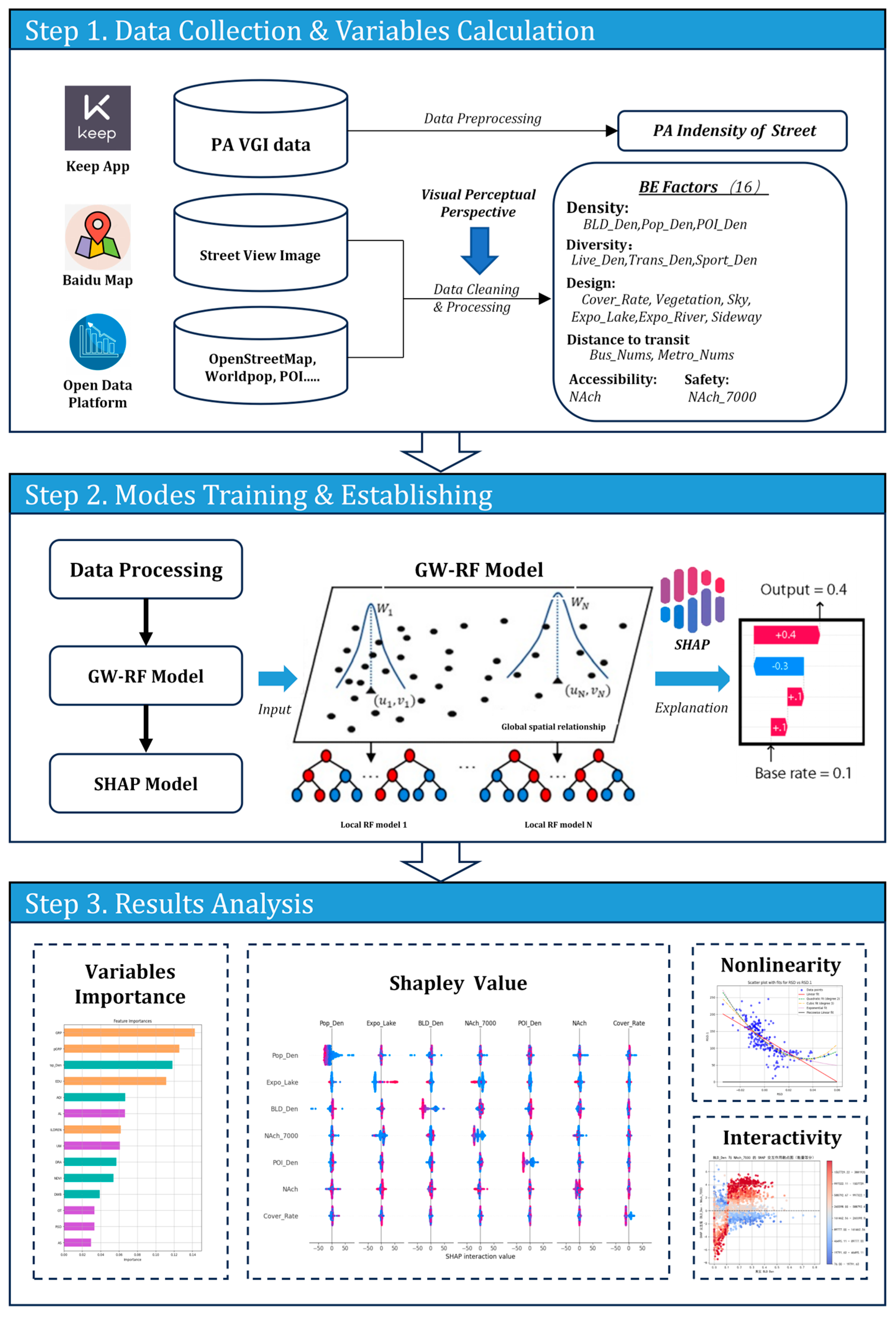
Figure 2.
The study area: main districts of Chengdu with a 1500m buffer.
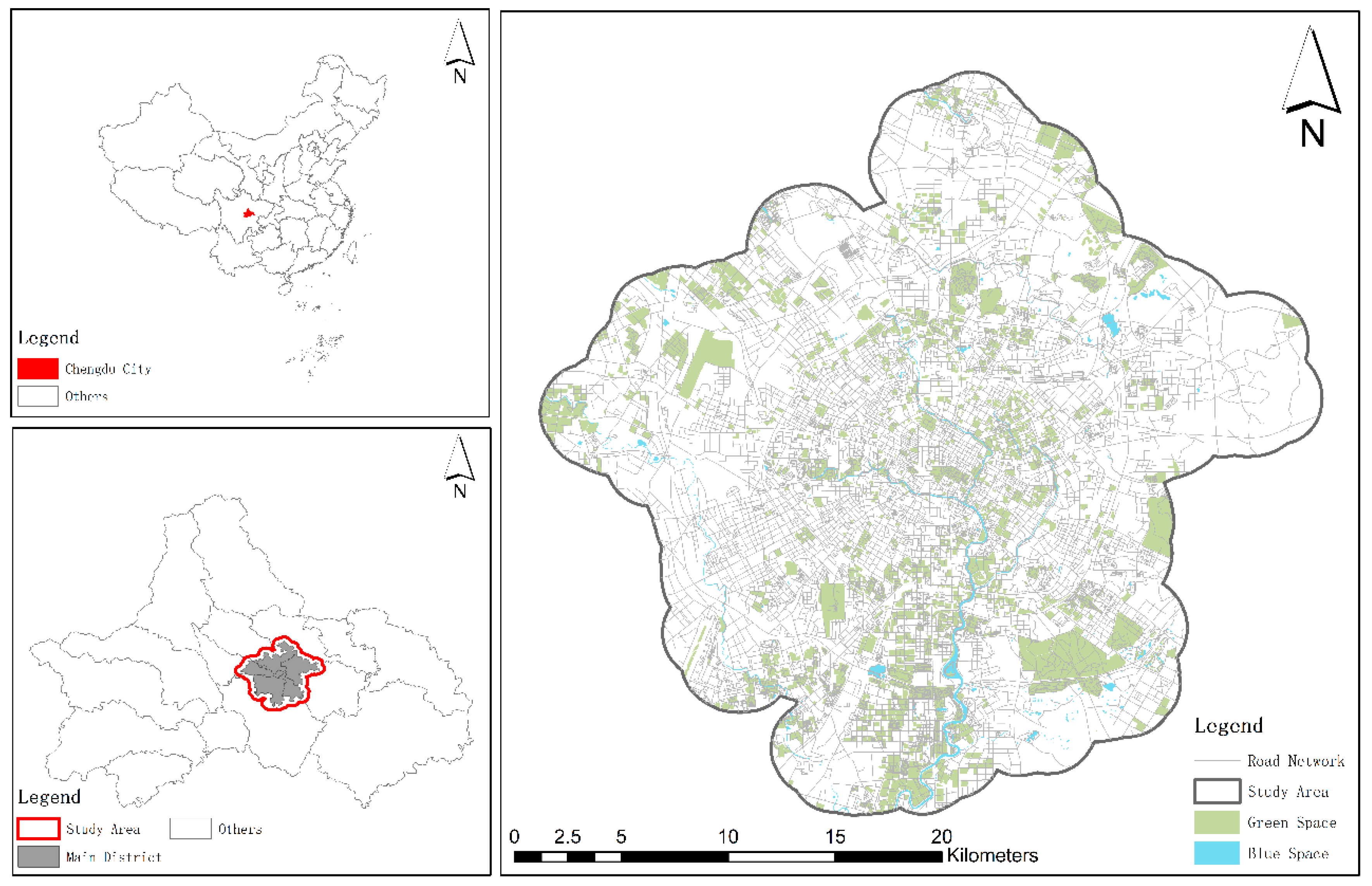
Figure 3.
Illustration of the vectorization results of popular routes.: (a) Route shapefile from the popular route data; (b) Vectorization results of the popular routes in ArcGIS platform (red indicates the street is passed by the route 2 times, green indicates the street segment is passed by the route 1 time).
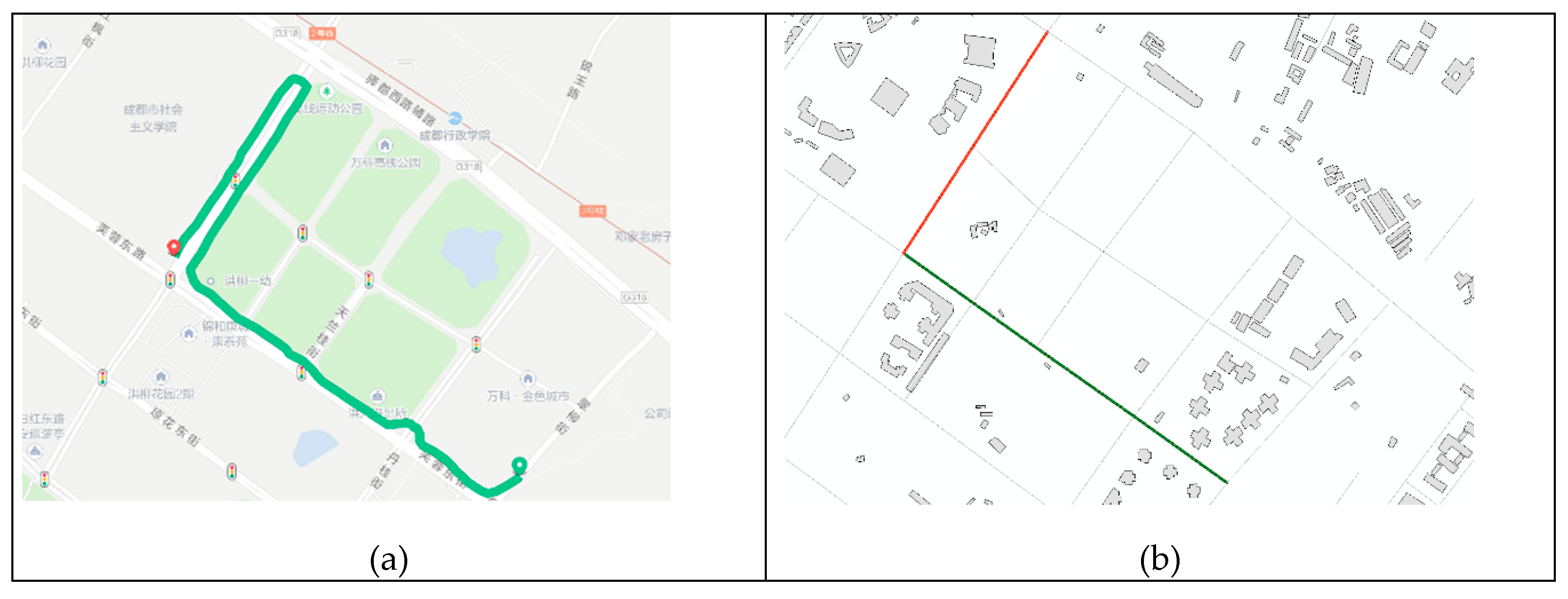
Figure 4.
Summary of the vectorization results of popular routes: (a) Spatial distribution of popular routes within the study area; (b) Illustration of the spatial relationship between polyline features and the converted point features.
Figure 4.
Summary of the vectorization results of popular routes: (a) Spatial distribution of popular routes within the study area; (b) Illustration of the spatial relationship between polyline features and the converted point features.
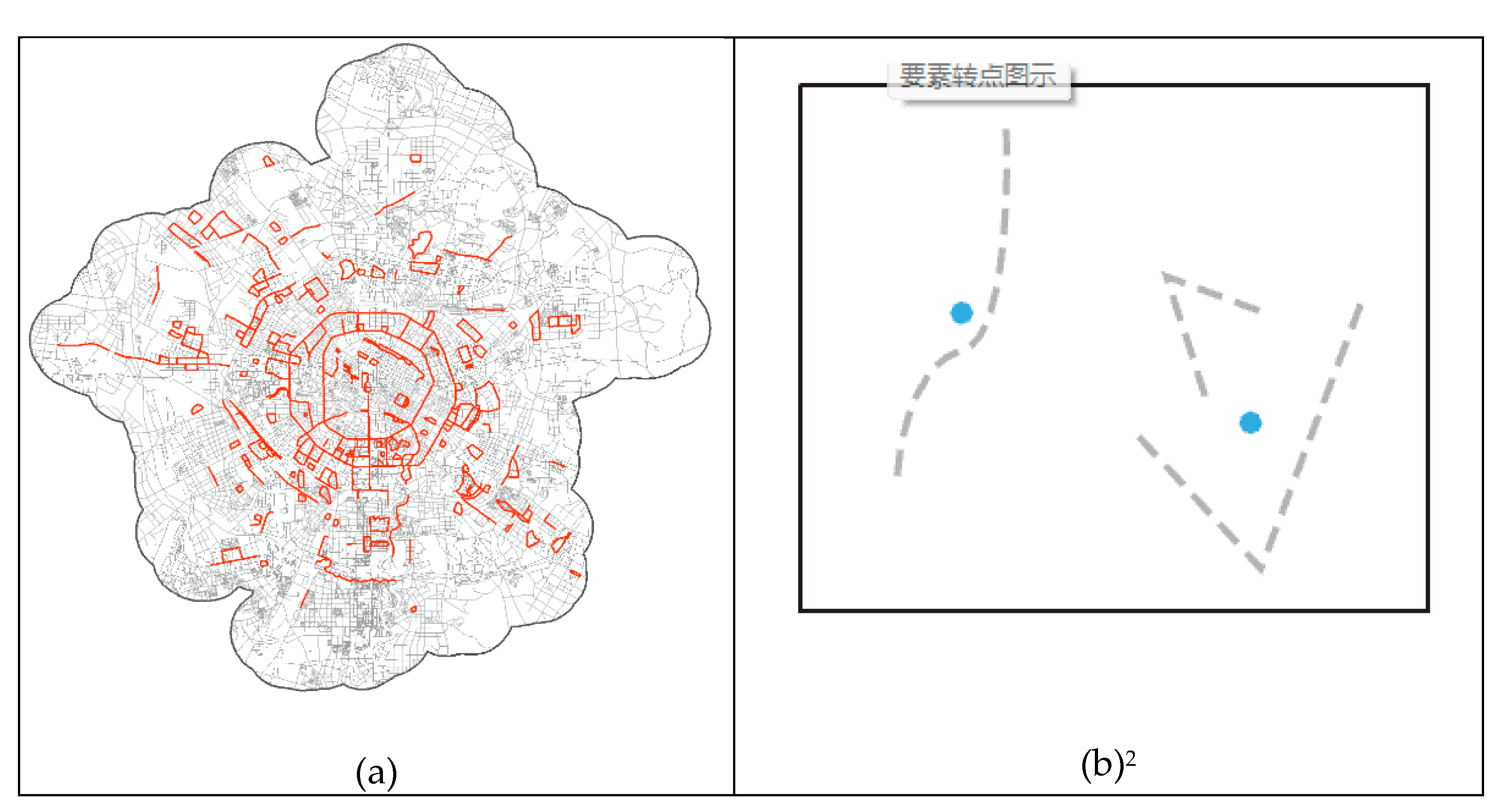
Figure 5.
Spatial distribution map of MPA intensity.
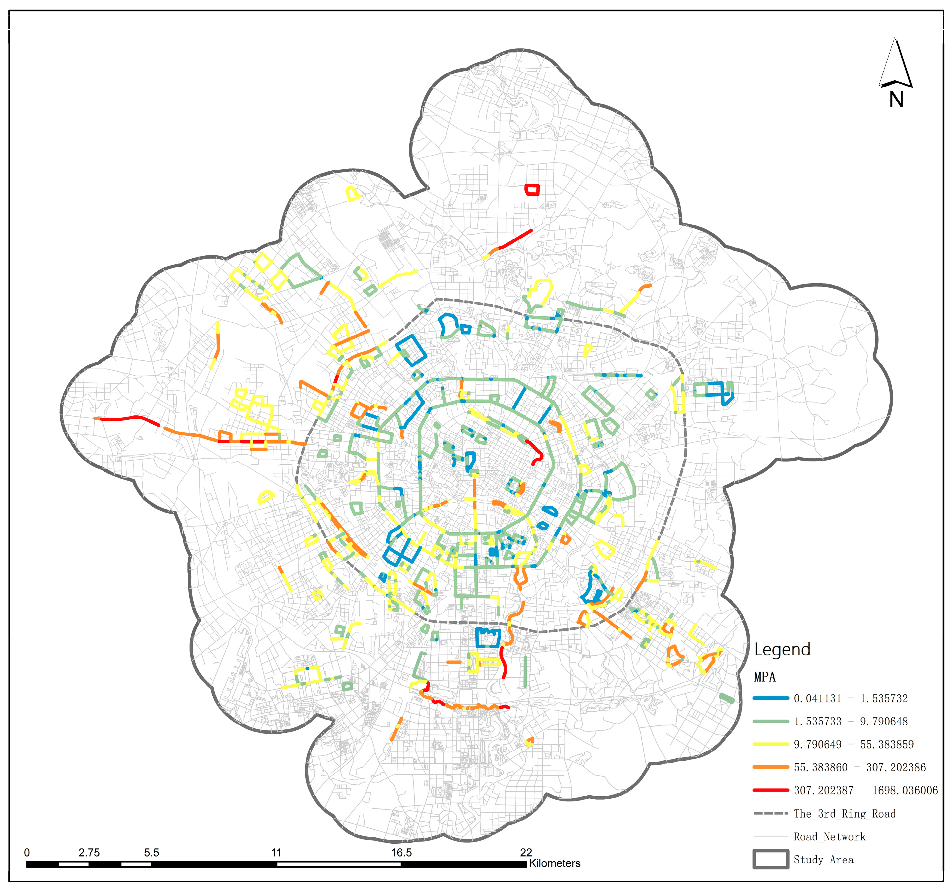
Figure 6.
Variables’ importance of the model.
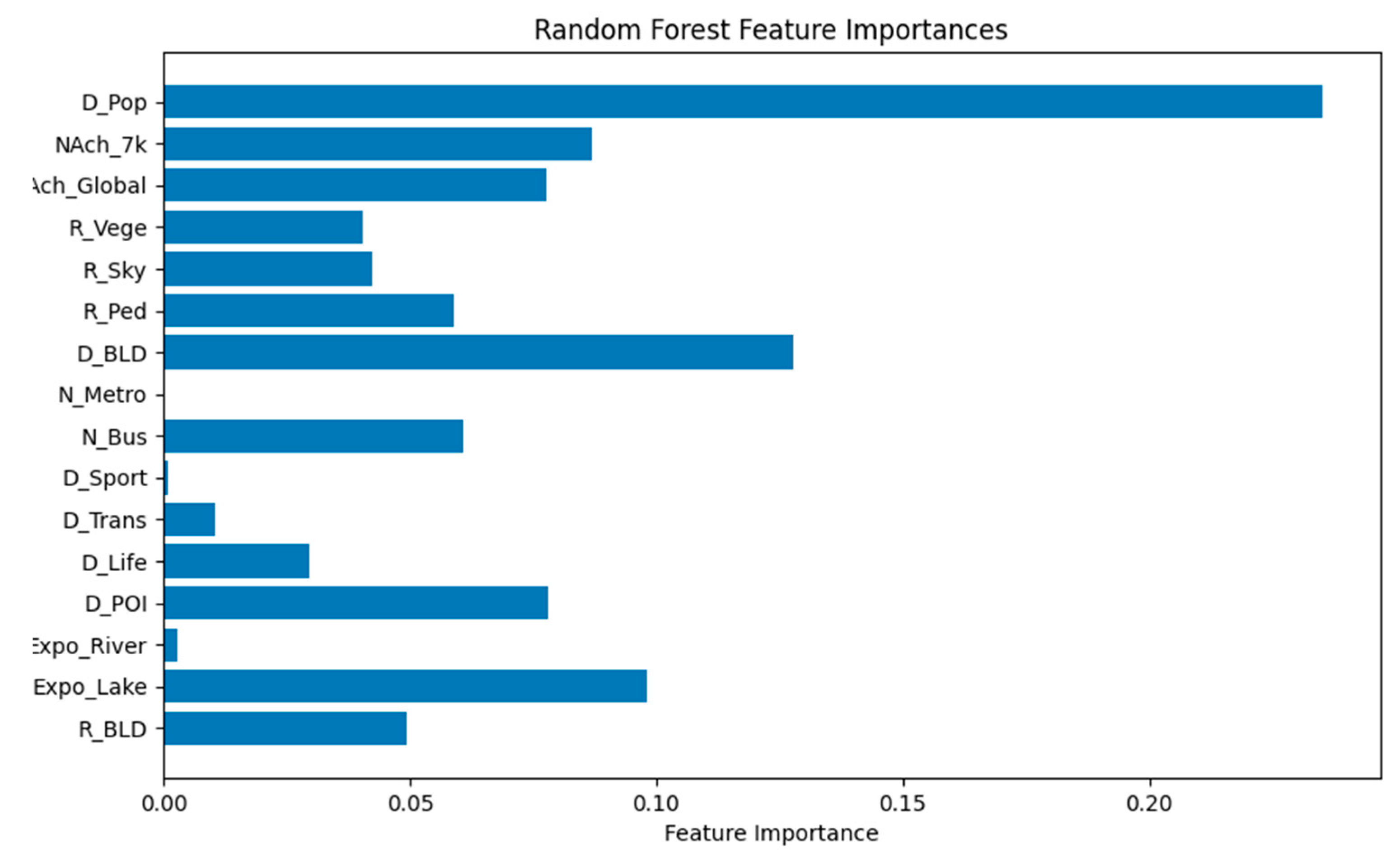
Figure 7.
SHAP summary plot: (a) SHAP summary plot for all samples; (b) SHAP summary plot after extreme value removal.
Figure 7.
SHAP summary plot: (a) SHAP summary plot for all samples; (b) SHAP summary plot after extreme value removal.
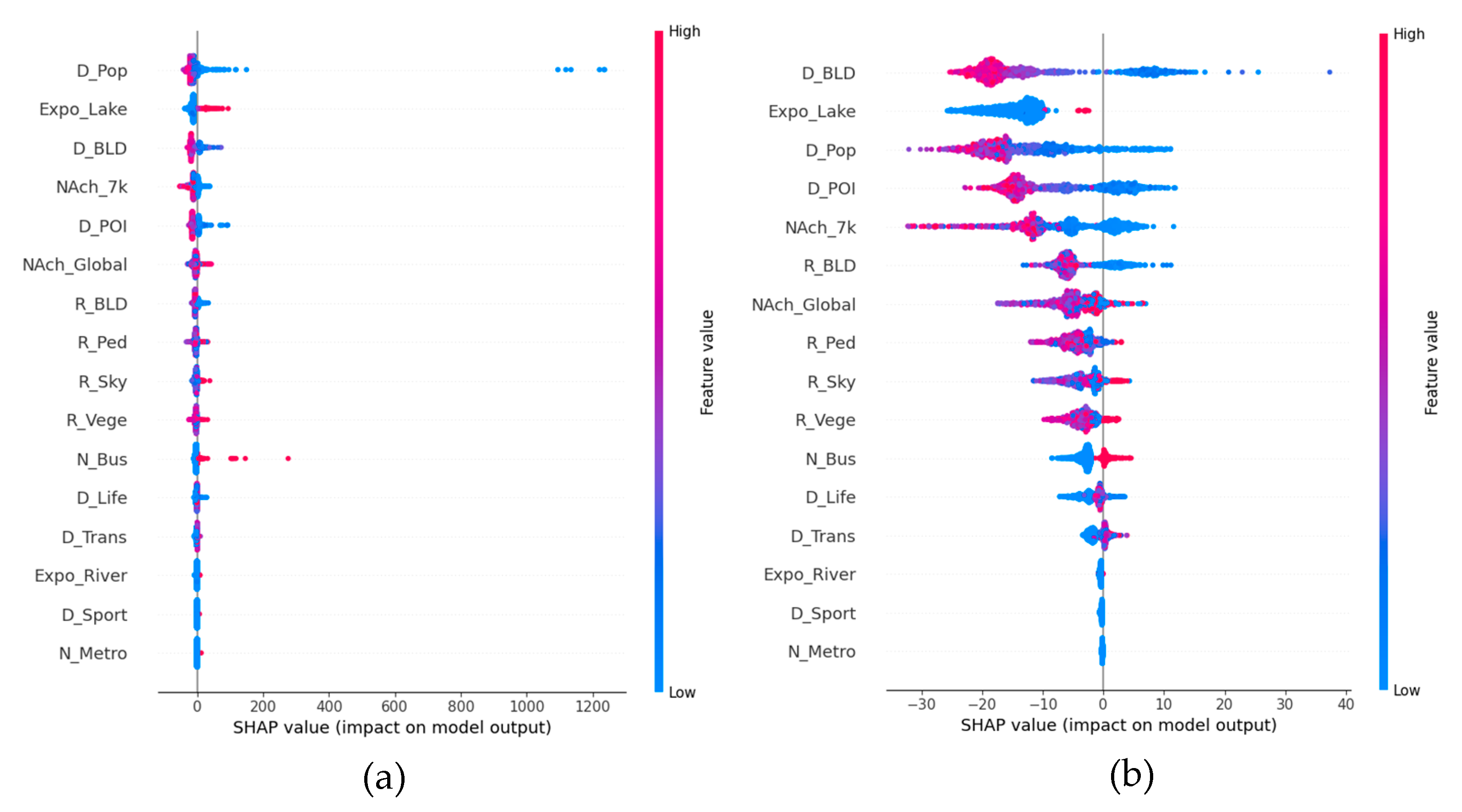
Figure 8.
Nonlinear Effects of Top 8 BE Variables. (The X-axis represents the actual values of the variables, and the Y-axis represents the SHAP values of the variables; a SHAP value greater than 0 indicates a positive contribution, while a value less than 0 indicates a negative contribution.).
Figure 8.
Nonlinear Effects of Top 8 BE Variables. (The X-axis represents the actual values of the variables, and the Y-axis represents the SHAP values of the variables; a SHAP value greater than 0 indicates a positive contribution, while a value less than 0 indicates a negative contribution.).
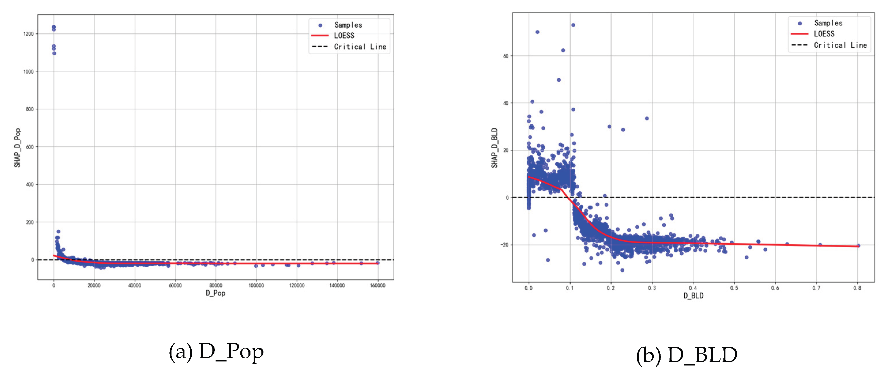
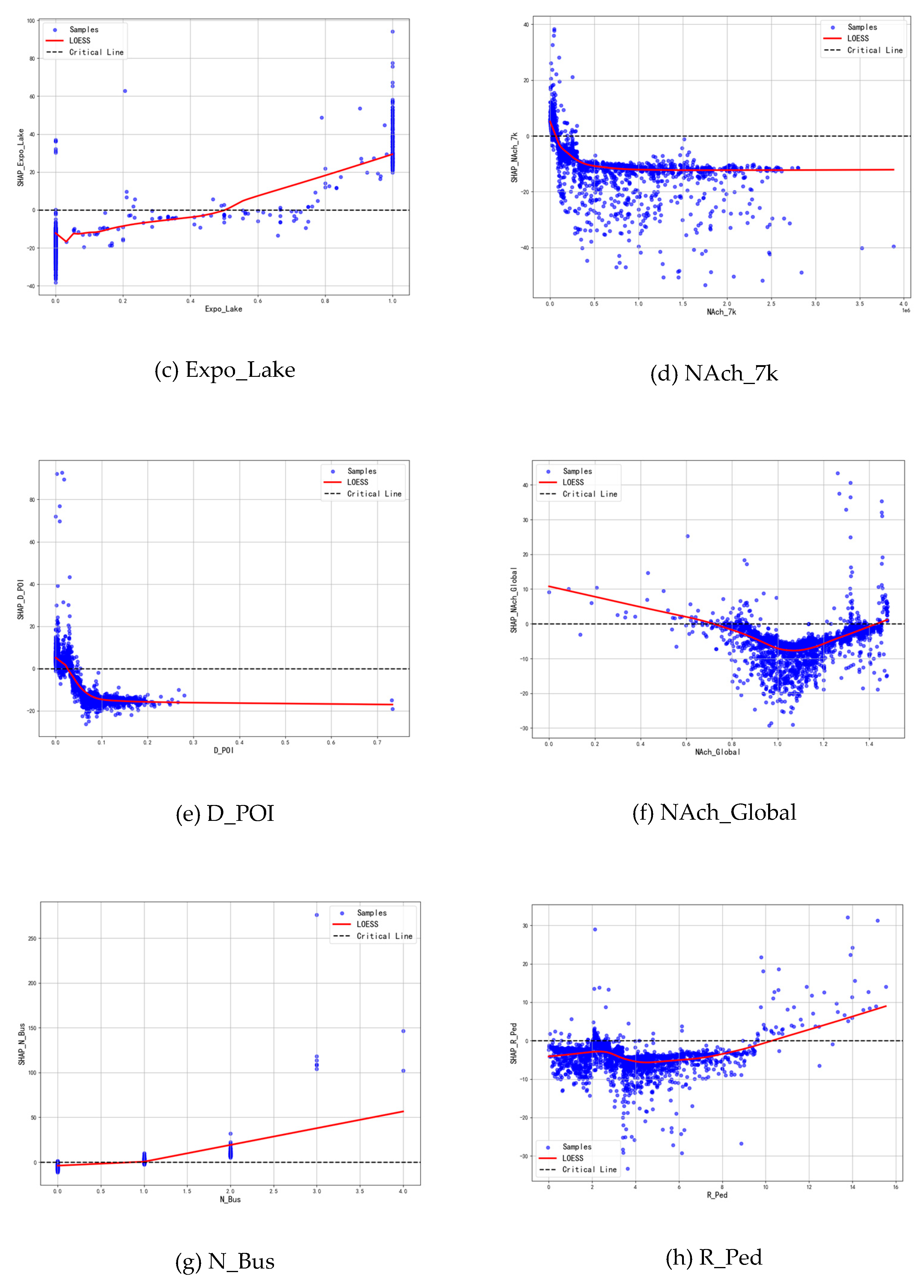
Figure 9.
SHAP summary plot of main effects and interaction effects.
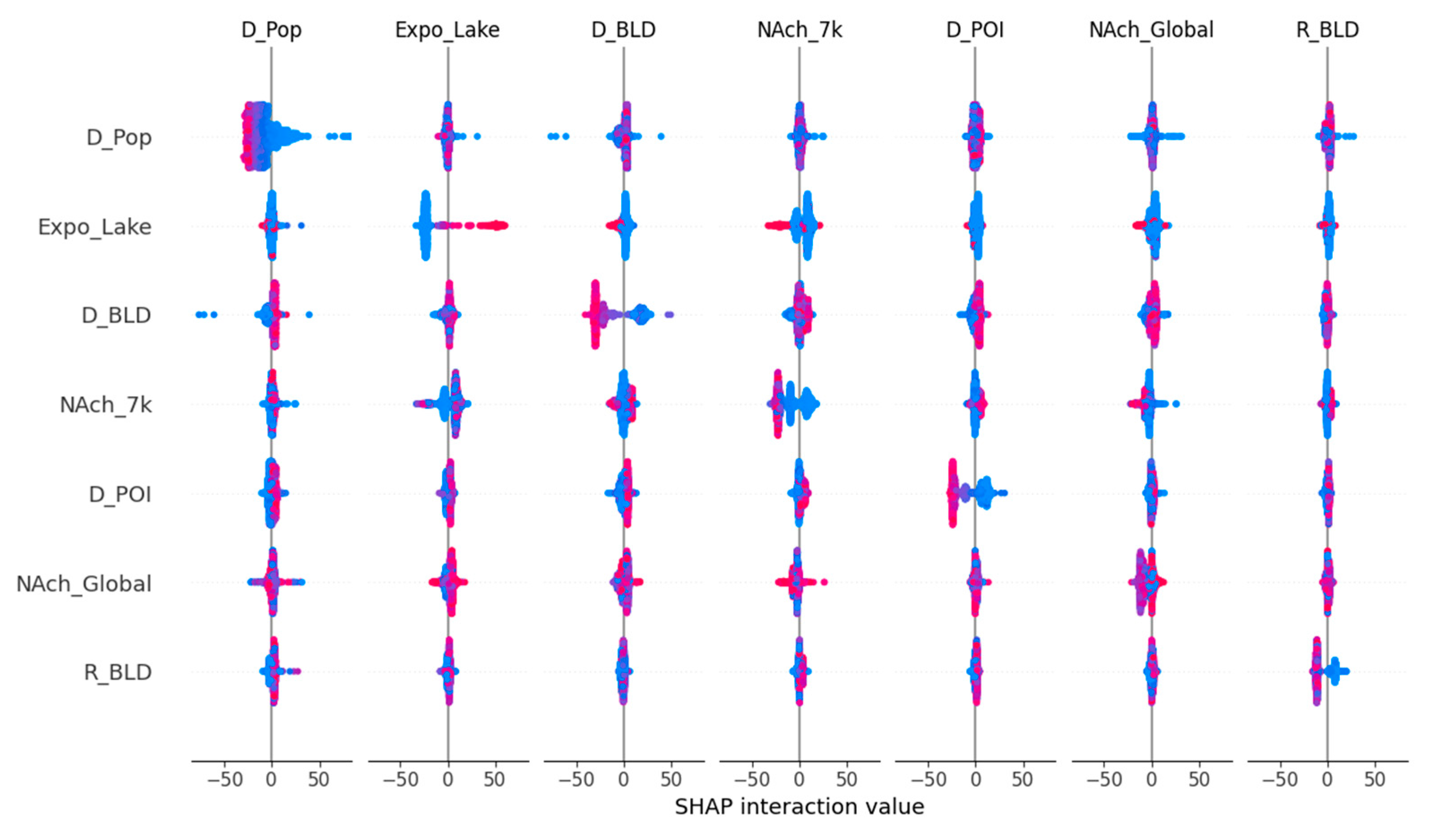
Figure 10.
Ranking of the importance of variables’ main effects.
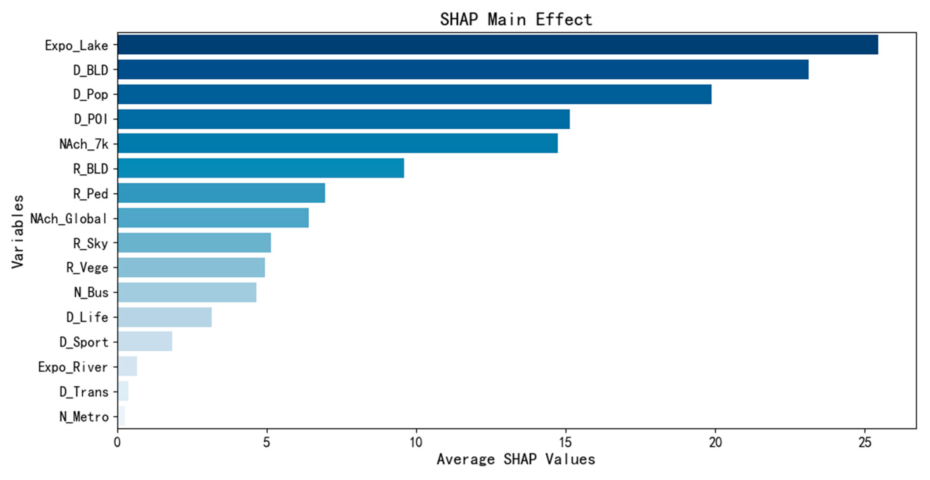
Figure 11.
Top 10 pairs of interaction variables by importance.
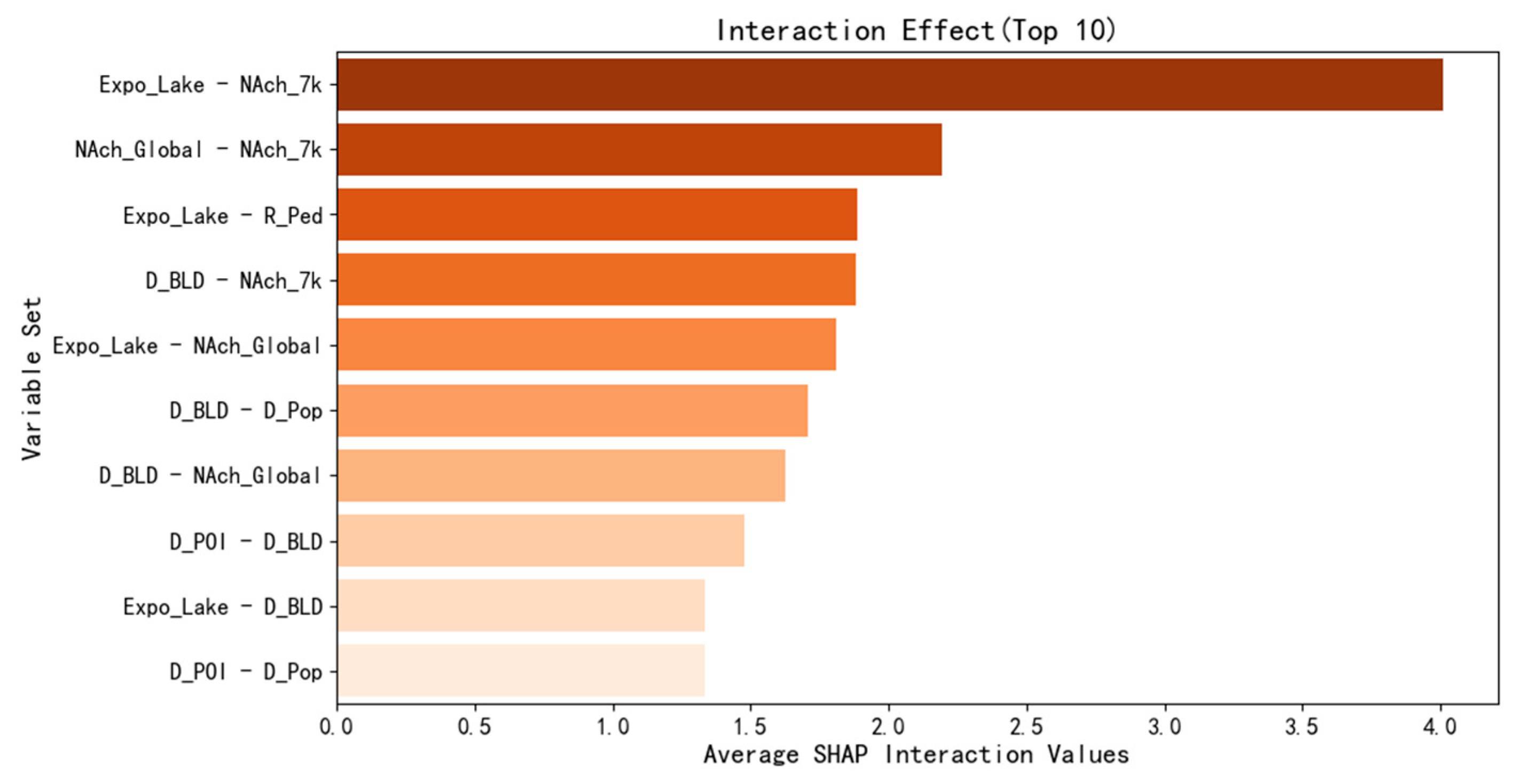
Figure 12.
Expo_Lake with other variables. (The X-axis represents the SHAP values of Variable A, and the Color Bar represents the SHAP values of Variable B; the Y-axis represents the interaction contribution value of this variable set. A Y-value greater than 0 indicates a positive interaction contribution, while a Y-value less than 0 indicates a negative interaction contribution.).
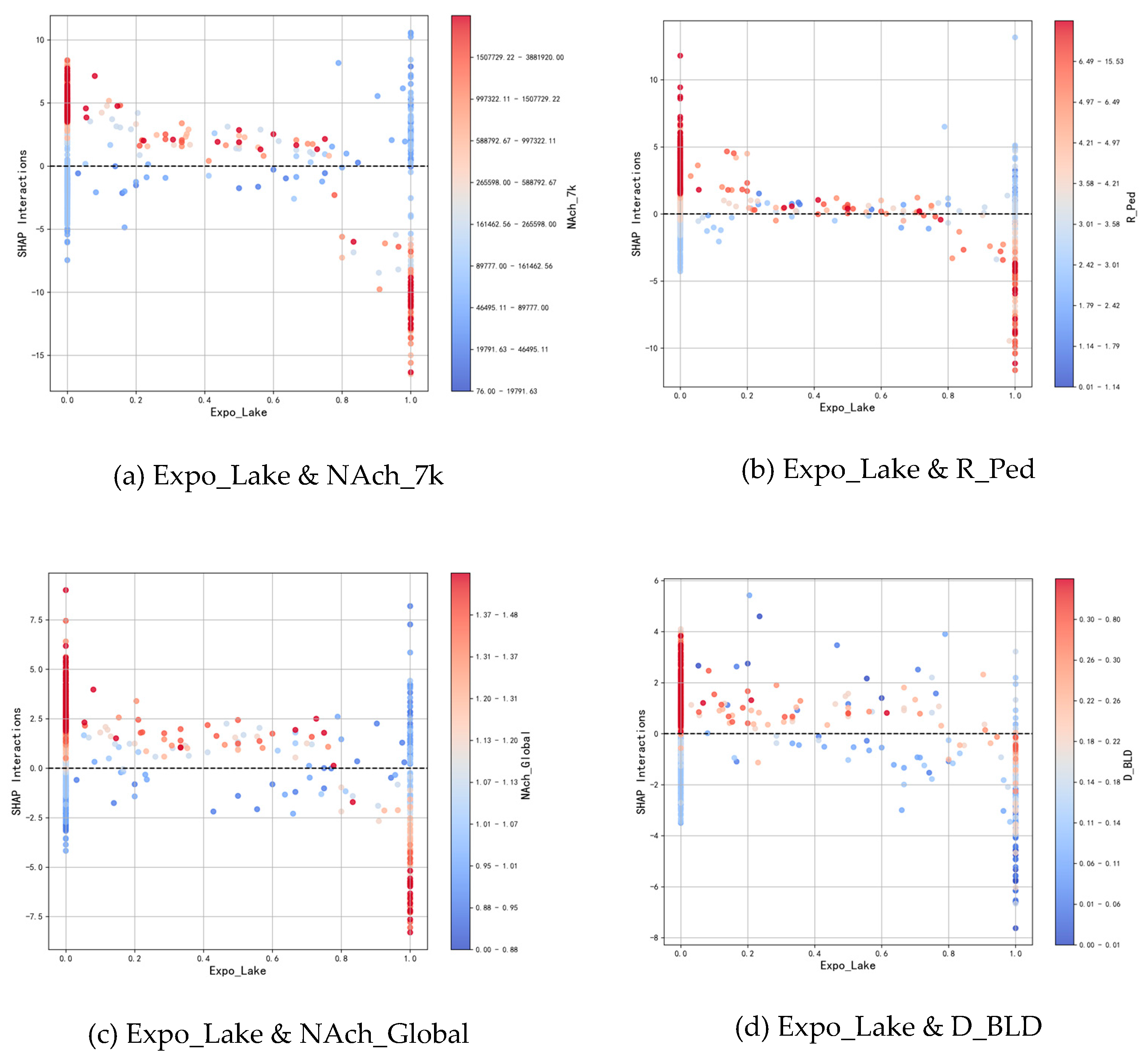
Figure 13.
D_BLD with other variables.

Figure 14.
D_Pop with other variables.
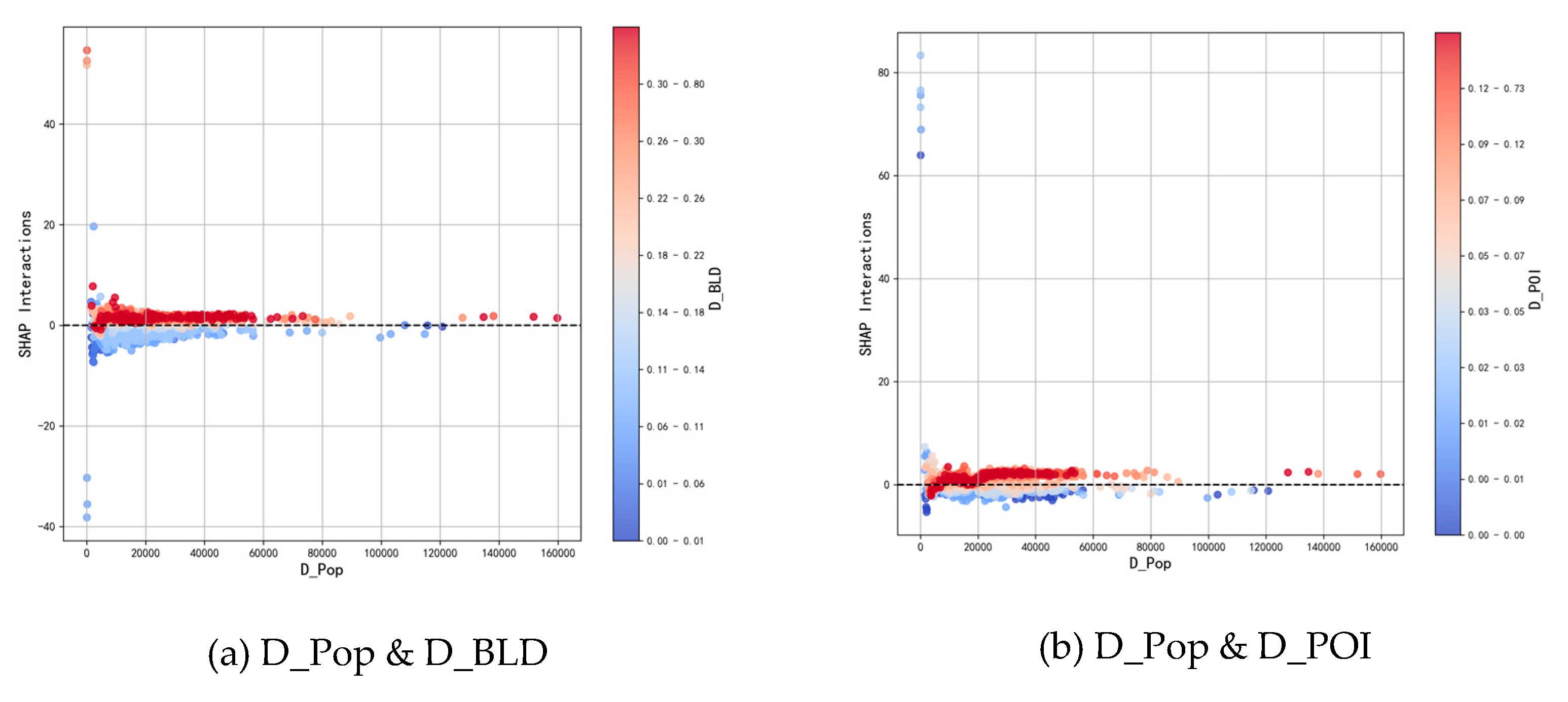
Figure 15.
NAch_Global with NAch_7k.
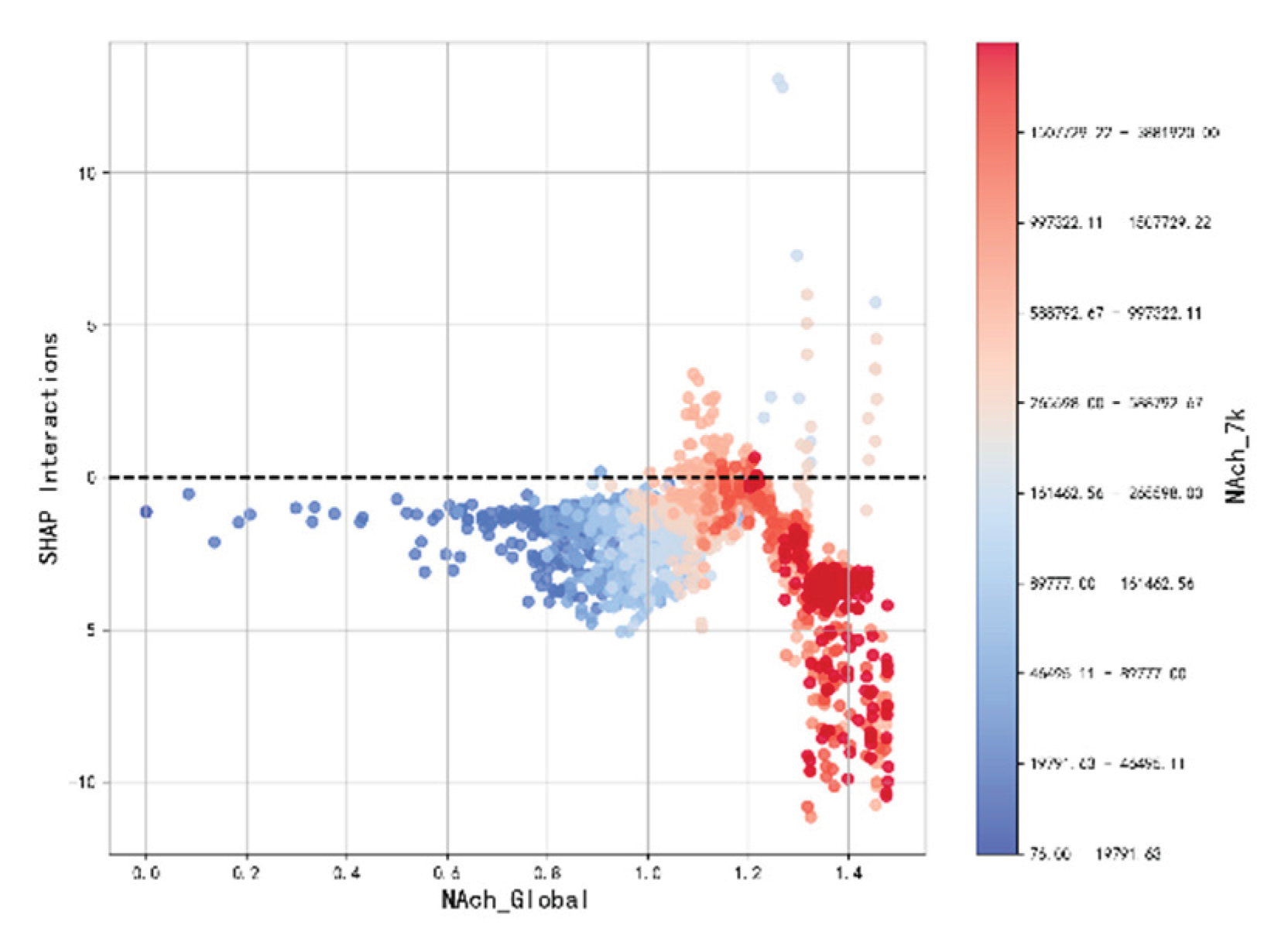

Table 1.
PA data descriptions.
| Information | Description | Sample |
|---|---|---|
| Route name | The custom name provided by the user when creating a route. | Vanke Loop Line |
| Route ID | Assigned by the system upon creation. | 5f145f0a88d6fe70e739556f |
| Route location | Geographical coordinates of the starting point of the route. | Longitude:30.5908 Latitude:104.1723 |
| Venue type | Including: Park, Street, Playground, Field and Others. | Street |
| Route length | - | 1671.2m |
| Check-in count | Cumulative check-ins since the creation of the route. | 814 times |
| Proportion of PA types | Proportion of running, walking, and cycling activities. | Running: 75% Walking: 9% Cycling: 16% |
| Route creation date | - | 2020-07-19, 22:56:10 |
| Route shape | The shape of the route on the online map. |  |
Table 2.
Data source descriptions.
| Data | Source | Recency | Accuracy |
|---|---|---|---|
| Road Network Data | Open Street Map3 | 2024.06 | - |
| Water Body Data | Open Street Map | 2024.06 | - |
| Population Raster Data | WorldPop4 | 2018 | 100m |
| Street View Image | Baidu Map5 | 2024.06 | - |
| Point of Interest | Gaode Map6 | 2024.06 | - |
| Building Footprint | Baidu Map | 2024.06 | - |
Table 3.
Definition and description of BE indicators.
| Dimensions | Variables | Abbr. | Description or calculation | Scale | Units |
|---|---|---|---|---|---|
| Density | Building Density | D_BLD | Building/Population/POI density within the street visual perception range. | 100m | % |
| Population Density | D_Pop | 100m | Persons/m2 | ||
| POI Density | D_POI | Along the Street | Nums/m | ||
| Diversity | Density of Life and Education-related POIs | D_Life | Types of POI density within the street visual perception range. | Along the Street | Nums/m |
| Density of Sports and Leisure-related POIs | D_Sport | ||||
| Density of Transportation-related POIs | D_Trans | ||||
| Design | Building Façade Enclosure | R_BLD | The ratio of total building façade width to street length. | Along the Street | % |
| Green View Ratio | R_Vege | The Proportion of Sky, Greenery, and Pedestrian Path Extracted from Street View Images. | - | ||
| Sky View Ratio | R_Sky | ||||
| Pedestrian Path Coverage Ratio | R_Ped | ||||
| Polygonal Water Exposure Ratio | Expo_Lake | The ratio of the area visible to pedestrians, where the view through buildings reveals water bodies, to the total length of the street. | 80m | ||
| Linear Water Exposure Ratio | Expo_River | 50m | |||
| Distance to Transit | Numbers of Bus Stops | N_Bus | The number of public transportation stops along the street. | Along the Street | Nums |
| Numbers of Metro Stations | N_Metro | ||||
| Accessibility | Road Network Accessibility | NAch_Global | Use the global and local NAch indicators from space syntax to express accessibility and simulate street motor vehicle flow. | Global | - |
| Safety | Simulated Traffic Flow in the Road Network | NAch_7k | 7000m | - |
Table 4.
The descriptive statistics of the BE indicators
| Dimensions | Indicators | Max | Min | Mean | Std.Dev | Units |
|---|---|---|---|---|---|---|
| Density | D_BLD | 100.00 | 0.00 | 17.11 | 0.14 | % |
| D_Pop | 186,191.09 | 25.87 | 14987.16 | 13711.98 | Persons/m2 | |
| D_POI | 6.92 | 0 | 0.05 | 0.09 | Nums/m | |
| Diversity | D_Life | 0.29 | 0 | 0.01 | 0.02 | Nums/m |
| D_Sport | 0.20 | 0 | 0.005 | 0.01 | ||
| D_Trans | 0.10 | 0 | 0.004 | 0.003 | ||
| Design | R_BLD | 99.55 | 0.00 | 20.26 | 0.20 | % |
| R_Vege | 91.12 | 0.00 | 27.02 | 0.12 | ||
| R_Sky | 44.50 | 0.00 | 8.69 | 0.07 | ||
| R_Ped | 17.06 | 0.00 | 3.31 | 0.02 | ||
| Expo_Lake | 100.00 | 0 | 5.28 | 0.20 | ||
| Expo_River | 100.00 | 0.00 | 10.27 | 0.28 | ||
| Distance to Transit | N_Bus | 5 | 0 | 0.15 | 0.42 | Nums |
| N_Metro | 8 | 0 | 0.04 | 0.31 | ||
| Accessibility | NAch_Global | 1.48 | 0 | 0.90 | 0.28 | - |
| Safety | NAch_7k | 3,907,158 | 0 | 174,492.87 | 377,905.64 |
Table 5.
Optimal bandwidth test results for the GW-RF model.
| Bandwidth | Model Performance | ||
|---|---|---|---|
| Max | Min | Std.Dev | |
| 1500m | 0.5605 | 20.65 | 56.74 |
| 1600m | 0.5668 | 20.15 | 56.34 |
| 1700m | 0.5546 | 20.79 | 57.12 |
| 1800m | 0.5852 | 20.12 | 55.13 |
| 1900m | 0.5690 | 21.12 | 56.19 |
| 2000m | 0.5643 | 20.26 | 56.50 |
Table 6.
Variables’ importance and ranking results.
| Dimensions | Variables | Importance Value | Ranking |
|---|---|---|---|
| Density | D_BLD | 0.1277 | 2 |
| D_Pop | 0.2351 | 1 | |
| D_POI | 0.0782 | 5 | |
| Diversity | D_Life | 0.0295 | 12 |
| D_Sport | 0.0008 | 15 | |
| D_Trans | 0.0105 | 13 | |
| Design | R_BLD | 0.0494 | 9 |
| R_Vege | 0.0405 | 11 | |
| R_Sky | 0.0423 | 10 | |
| R_Ped | 0.0513 | 9 | |
| Expo_Lake | 0.0982 | 3 | |
| Expo_River | 0.0030 | 14 | |
| Distance to Transit | N_Bus | 0.0608 | 7 |
| N_Metro | 0.0004 | 16 | |
| Accessibility | NAch_Global | 0.0778 | 6 |
| Safety | NAch_7k | 0.0870 | 4 |
Table 7.
Comparison between the main effects of certain variables and the global variable importance ranking.
Table 7.
Comparison between the main effects of certain variables and the global variable importance ranking.
| Variables | Ranking of Main Effects | Ranking of Global Importance |
|---|---|---|
| Expo_Lake | 1 | 3 |
| D_BLD | 2 | 2 |
| D_Pop | 3 | 1 |
| D_POI | 4 | 5 |
| Nach_7k | 5 | 4 |
| R_BLD | 6 | 9 |
| R_Ped | 7 | 8 |
| NAch_Global | 8 | 6 |
Disclaimer/Publisher’s Note: The statements, opinions and data contained in all publications are solely those of the individual author(s) and contributor(s) and not of MDPI and/or the editor(s). MDPI and/or the editor(s) disclaim responsibility for any injury to people or property resulting from any ideas, methods, instructions or products referred to in the content. |
© 2025 by the authors. Licensee MDPI, Basel, Switzerland. This article is an open access article distributed under the terms and conditions of the Creative Commons Attribution (CC BY) license (http://creativecommons.org/licenses/by/4.0/).
Copyright: This open access article is published under a Creative Commons CC BY 4.0 license, which permit the free download, distribution, and reuse, provided that the author and preprint are cited in any reuse.


