
Submitted:
16 October 2025
Posted:
17 October 2025
You are already at the latest version
Abstract
Geographic Information Systems (GIS) have consolidated as essential analytical tools for addressing public health and urban security challenges, yet the available evidence remains fragmented due to methodological heterogeneity and geographical inequalities. This study applied a fused pipeline integrating Systematic Mapping (SM) and Systematic Review (SR), grounded in the PICOS (health) and SPICE (security) frameworks, which systematically reduced an initial corpus of 7,106 records to 65 core articles through multi-layered screening and a 1–4 technical quality scoring matrix. Results indicate sustained growth in scientific production, peaking in 2023 (32.3% of all publications). Geographically, research is concentrated in Asia (33.8%) and North America (16.9%), while Africa (12.3%) and South America (9.2%) remain underrepresented. Methodologically, a dominant core was identified around accessibility metrics (36.9%) and spatial autocorrelation (27.7%), with a prevalence of cross-sectional observational designs and limited adoption of advanced models such as Bayesian inference and machine learning (9.2%). The technological ecosystem is dominated by ArcGIS (61.5%) and QGIS (23.1%), complemented by open-source environments such as R, Python, and SaTScan. Overall, the fused SM+SR pipeline provides a transparent and replicable framework that exposes key strengths—high spatiotemporal resolution and scalability—while revealing critical gaps related to data openness and reproducible validation, offering concrete guidelines for future research and evidence-based policymaking.
Keywords:
Geographic Information Systems (GIS)
; systematic mapping
; systematic review
; public health
; urban security
; spatial epidemiology
; accessibility analysis
; spatial autocorrelation
; PICOS
; SPICE
1. Introduction
Geographic Information Systems (GIS) have become essential tools for understanding the complex interactions between health, environment, and urban security. Their capacity to integrate spatial, temporal, and multivariate data has enabled significant advances in spatial epidemiology, healthcare accessibility, disease surveillance, and crime prevention. Nevertheless, the field remains fragmented, with marked heterogeneity in data quality, study designs, and methodological approaches.
Recent studies have demonstrated that, although Geographic Information Systems (GIS) have proven effective in identifying spatial patterns of health inequities and risk distribution across diverse populations [1,2,3], persistent methodological and contextual limitations continue to constrain the generalizability of these findings—particularly in low- and middle-income settings where data completeness and comparability remain limited [4,5]. Similarly, in the domain of urban security, spatial modeling approaches have been recognized for their technological innovation and contribution to predictive analytics [6,7], yet they have also been questioned for their ethical implications, methodological biases, and risks of poor replicability [8,9].
Against this backdrop, the present study introduces a fused pipeline combining Systematic Mapping (SM) and Systematic Review (SR), designed to characterize the available evidence, identify recurrent strengths and limitations, and highlight critical research gaps. As an added value, the study applies internationally recognized frameworks—PICOS for public health and SPICE for urban security—thus ensuring traceability, comparability, and reproducibility of the results.
To complete the methodological framework, the analytical narrative is organized into three complementary levels—descriptive, intermediate, and advanced—corresponding to the needs of early-stage researchers (ESR), mid-career researchers (MCR), and senior researchers (SR). This design not only guarantees a comprehensive synthesis but also facilitates the transfer of knowledge across diverse professional and scientific audiences, thereby strengthening the relevance of GIS-based evidence in both health and urban security domains.
Previous evidence synthesis studies have rigorously applied PRISMA and PICOS frameworks to ensure methodological transparency and reproducibility in domains such as medical image processing and sensor-based cancer detection [10,11]. These works established a robust methodological foundation and demonstrated the applicability of systematic evidence synthesis in biomedical research. Building upon this foundation, the present study expands the scope to the health domain, providing a broader analytical perspective and addressing research gaps that remain underexplored in the current literature.
In this study, GIS are conceptualized as programmable analytical environments that integrate vector and raster operations, spatial statistics, and open data workflows. Under the PRISMA–PICOS/SPICE framework, the software environments employed (ArcGIS, QGIS, R, Python, and SaTScan) and their coordinate reference systems (CRS) are explicitly documented to ensure geocomputational reproducibility. This approach establishes a technological bridge between spatial modeling and its applications in public health and urban security, where transparency and replicability serve as core scientific principles for long-term methodological synthesis.
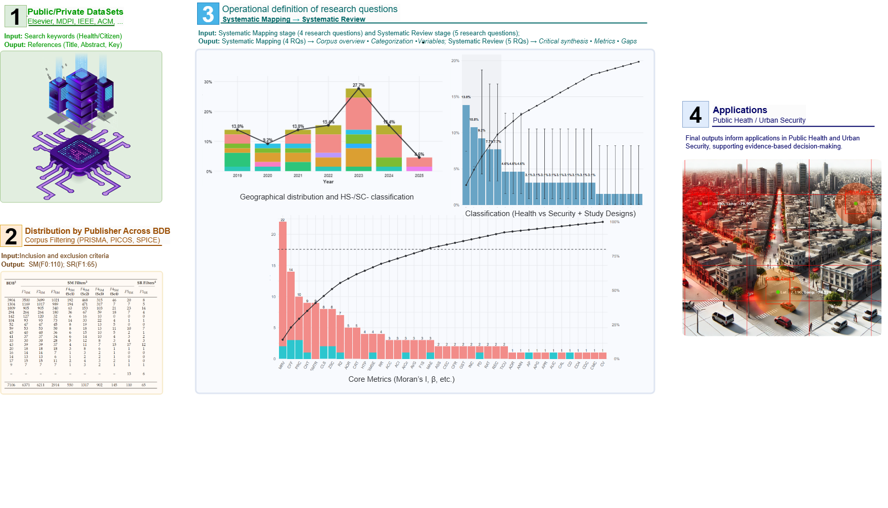
2. Baseline Benchmark of the Systematic Mapping and Review Corpus
2.1. Public and Private Data Sources
The main public databases used in the publications included in this research are summarized below. Each dataset is reported following the producing agency, year, and official documentation, ensuring transparency and traceability.
DBO49 – The DHS Program. This program provides country-specific survey reports with their own bibliographic references; there is no single DOI or generic citation for the dataset. References must therefore cite the country, year, and producing agency.
Ethiopia DHS 2016. Ethiopia Demographic and Health Survey 2016 [Dataset]. Women aged 15–49 receiving antenatal care from skilled personnel increased from 27% in 2000 to 62% in 2016, although only 32% achieved four or more visits. The most frequent controls were blood pressure (75%) and blood testing (73%), followed by urine analysis and nutritional counseling (66%). Institutional deliveries rose from 5% (2000) to 26% (2016), while home births decreased from 95% to 74%. Postnatal care within the first two days was received by 17% of women and 13% of newborns. Barriers to accessing medical care fell from 96% in 2005 to 70% in 20161 [12].
India NFHS-5 (2019–21). International Institute for Population Sciences (IIPS) and ICF. India National Family Health Survey (NFHS-5), 2019–21 [Dataset]. Fieldwork was conducted in two phases: Phase I (June 2019–January 2020) covering 17 states and 5 Union Territories, and Phase II (January 2020–April 2021) covering 11 states and 3 Union Territories. Data collection involved 636,699 households, 724,115 women, and 101,839 men2 [13].
Uganda DHS 2016. Uganda Bureau of Statistics (UBOS) and ICF. Uganda Demographic and Health Survey 2016 [Dataset]. Kampala, Uganda, and Rockville, Maryland, USA: UBOS and ICF. The survey shows progress in family planning indicators: modern contraceptive use among married women increased from 14% (2000–2001) to 35% (2016), with injectables as the most common method. However, discontinuation rates remained high (45% stopped within 12 months, mostly due to health concerns or side effects). Total demand for family planning rose from 54% to 67%, but only 52% was met by modern methods. Unmet need persisted (28% of married and 32% of sexually active single women). Among non-users, 64% expressed future intention to use contraceptives3 [14].
Cameroon DHS 2018. Cameroon Demographic and Health Survey 2018 [Dataset]. The survey highlights relatively high knowledge of HIV prevention, but marked inequalities by education and gender. While 70% of individuals aged 15–49 acknowledged condom use and monogamy reduce infection risk, only 42% of uneducated men knew this, compared to 85% with higher education. Regarding mother-to-child transmission, 71% of women and 68% of men recognized pregnancy as a risk period, and three-quarters of women reported awareness of antiretroviral use. Behavioral indicators show that 22% of women and 38% of men reported non-marital sex in the past year, with condom use limited (43% in women and 63% in men). Lifetime sexual partners differed by gender (4.2 in women vs. 9.7 in men). Although nearly 90% knew where to get tested, 29% of women and 43% of men had never been tested; among those tested, 40% of women and 34% of men did so in the previous year. Coverage of HIV counseling during antenatal care reached 55% of pregnant women4 [15].
DBO41 – IBGE, Brazil Census 2010. Sinopse do Censo Demográfico 2010 [Dataset]. Brazil reached 5,565 municipalities in 2010, with higher concentration in the Northeast (32%) and Southeast (30%). Minas Gerais stood out as the state with the largest number of municipalities (853)5 [16].
DBO8 – WorldPop Hub. Estimated total number of people per grid-cell [Dataset]. Data are available in GeoTIFF format at a resolution of 3 arc-seconds (approx. 100m at the equator), using a Geographic Coordinate System (WGS84). Units are number of people per pixel, derived from Random Forest-based dasymetric redistribution6 [17].
In contrast to these public datasets, private or licensed datasets were used in 29 studies, with access restricted to the producing institutions or the participating research teams. This condition inherently limits independent replication and reduces methodological transparency. Within this group, some studies relied exclusively on proprietary experimental datasets generated by the authors themselves, which reinforces the contextual validity of findings by ensuring direct control over data collection and processing, but at the same time restricts external verification and complicates cross-study comparability.
Beyond these qualitative descriptions of the three most relevant datasets, the systematic mapping also quantified the overall distribution of datasets across the 65 included articles. Figure 1 summarizes these findings: panel ( 1a) shows the top-10 public datasets, dominated by large-scale demographic surveys such as DHS (DBO49) and census-based sources like IBGE (DBO41), alongside global population grids (WorldPop, DBO8). Panel ( 1b) illustrates the distribution of private datasets, where a single source (DBP5) accounts for more than 85% of the cases. This contrast highlights both the diversity and openness of public data, as well as the concentration and restricted accessibility of private sources, with direct implications for replicability and transparency.
GIS provide a methodological framework to integrate, manage, and transform georeferenced data from multiple sources. As summarized in Figure 2 and detailed in Table 1, the framework links software ecosystems to analytical domains (Health and Urban Safety) and spatial techniques, providing the technological baseline for the review. Examples across public health include spatio-temporal pandemic analyses [18], optimization of prehospital coverage [2], interpolation of pollutants such as PM2.5 [3], and vector-borne risk assessment (e.g., dengue) [19]; within security, GIS support crime mapping, hotspot identification, and predictive modeling [6,20,21], as well as protection of critical infrastructures and territorial resilience [22]. The decision-support potential of GIS depends on data quality/resolution and the robustness of applied models, including the translation of analytical outputs into operational interventions [8,23,24,25,26].
2.2. Technological Benchmark: Integration of Software and Spatial Techniques
This subsection establishes the technological baseline of the analytical ecosystem identified across the corpus of 65 studies. It characterizes the diversity of software environments and spatial analytical approaches used to address health- and security-related problems through GIS. The analysis integrates three complementary dimensions: (i) the type of GIS and computational environments employed, (ii) the methodological domains in which they operate, and (iii) the spatial techniques most frequently applied within each ecosystem.
The corpus reveals a balanced yet heterogeneous technological landscape in which proprietary GIS and statistical packages (e.g., ArcGIS, IBM SPSS, Stata) coexist with open-source environments (QGIS, R, Python, GeoDa, SaTScan). Each platform is associated with specific analytical strengths: for instance, ArcGIS and QGIS dominate in cartographic visualization and network-based accessibility analysis, GeoDa and R support inferential spatial statistics (e.g., Moran’s I, LISA, GWR), and SaTScan specializes in cluster detection using Poisson or Bernoulli models. Python environments extend this ecosystem through automated processing, machine learning, and spatial data integration workflows.
Figure 2.
Conceptual GIS integration framework: schematic taxonomy linking software ecosystems, analytical domains (Health and Urban Safety), and spatial techniques. This model guides reproducibility verification (Section 3.4) and the quantitative synthesis of technological ecosystems (Section 4.2.3).
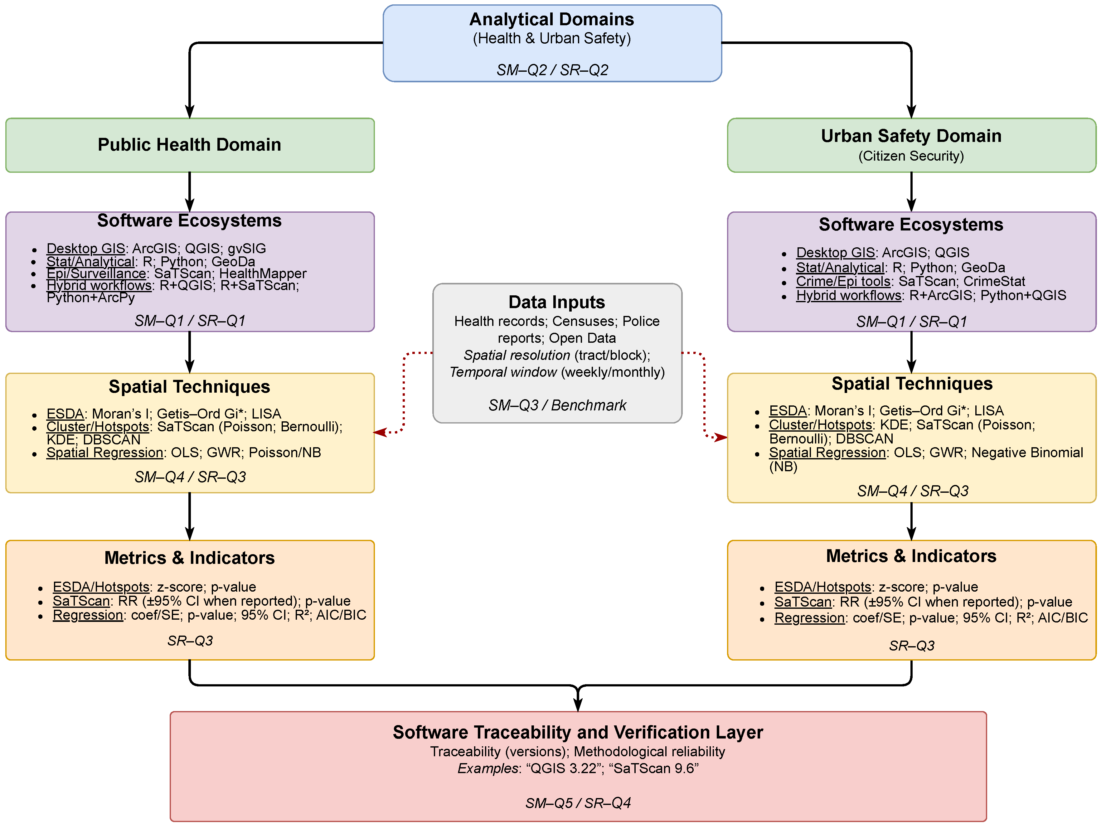

Table 1.
GIS and computational environments identified in the corpus. Dominant techniques correspond to the most frequent spatial analyses associated with each ecosystem.
Table 1.
GIS and computational environments identified in the corpus. Dominant techniques correspond to the most frequent spatial analyses associated with each ecosystem.
| Software / Platform | Dominant Spatial Techniques and Applications | Category |
|---|---|---|
| ArcGIS (Esri) | Hotspot mapping, network analysis, raster interpolation, polygon overlay | Proprietary GIS |
| QGIS (Open source) | Geoprocessing, density mapping, accessibility surfaces, visualization | Open-source GIS |
| GeoDa | Spatial weights matrices, LISA, spatial regression (OLS, GWR) | Open-source analytics |
| SaTScan | Space–time cluster detection (Poisson, Bernoulli) | Specialized cluster analysis |
| R (CRAN ecosystem) | Spatial regression, kriging, simulation, spatial autocorrelation | Statistical computing |
| Python (Anaconda / Jupyter) | Machine learning, geoprocessing, automated workflows | Open-source programming |
| Stata | Spatial econometrics, health-risk modeling | Proprietary statistics |
| IBM SPSS | Descriptive and inferential modeling | Proprietary statistics |
Table 2.
Operational definition of variables derived from research questions in the fused pipeline (SM→SR).
Table 2.
Operational definition of variables derived from research questions in the fused pipeline (SM→SR).
| Variable (with guiding question in context) | Operational / Source in dataset | Level1 |
|---|---|---|
| Systematic Mapping (SM) | ||
|
Scientific production : In which years and regions is the production of GIS-related articles in public health and citizen security concentrated? |
Publication year of each record + Country/Region | ESR |
| As summarized in Table 2, this dual organization serves a twofold purpose: framing the analytical scope of the study and providing an operational dictionary of variables applied consistently throughout the fused pipeline (SM→SR). In practice, the table functions simultaneously as a framework of research questions and as a concrete guide for variable extraction. Application scenarios : Which urban/rural/regional settings predominate, and how are they distributed between health and security studies? |
Application scenario (SPICE–Setting) + Theme [health vs. security] | ESR |
|
CTechniques and metrics applied : What combinations of study type and methodological design predominate in the GIS literature applied to public health and citizen security, and which are the most frequent within the analyzed corpus? |
Study type × Methodological design | MCR |
|
Publication channels : Which journals and categories publish the greatest volume, and which concentrate the core high–impact GIS and health/security articles? |
Journal × Publisher × Quartile × Impact Factor | SR |
| Systematic Review (SR) | ||
|
Simple metrics : How is the use of standardized metrics organized across the recent literature, and what differences emerge across application areas? |
Cross-sectional distribution (top vs. long tail), domain split (Health vs. Public Safety), Pareto concentration. | ESR |
|
Temporal and domain dynamics : How is the use of standardized metrics characterized, and how does it change across domains and over time? |
Period bins (2019 – 2024); proportions with 95% Wilson CIs; Health vs. Public Safety comparison | ESR |
|
Software tools and platforms : Which software tools, platforms, and libraries are most frequently reported in GIS-based health and public-safety studies, and how concentrated is their usage? |
Tools (GIS desktop/platforms, statistics/data analysis, spreadsheets, portals/viewers, programming languages, geospatial libraries, APIs, databases, image processing) + Frequency (%) | MCR |
|
Inferential techniques + outcomes : Which inferential spatial techniques are applied and with what results? |
Technique (Moran’s I, Gi*, SaTScan, E2SFCA, AUC, regressions) + Outcomes (OR, RR, coefficients, AI, CFR) | MCR |
|
Methodological assessment : Which methodological strengths, limitations, and research gaps predominate in the GIS health/public-safety literature, and which Limitation–Gap pairs show non-random co-occurrence, indicating priorities to improve replicability and validity? |
Strengths vs. weaknesses (resolution, cost, bias, data scarcity) | SR |
1 ESR=Early-Stage Researchers, MCR=Mid-Career Researchers, SR=Senior Researchers.
Overall, this technological benchmark consolidates a descriptive foundation for understanding how GIS environments, computational tools, and spatial methodologies converge across domains. By clarifying these associations, it provides the conceptual groundwork for assessing reproducibility and methodological consistency in subsequent sections of this study. Importantly, this benchmark also establishes the structural context for the inferential analyses developed in Section 4.2.4, where the spatial techniques identified here (e.g., Moran’s I, Getis–Ord Gi*, SaTScan, GWR, OLS, Poisson models) are quantitatively evaluated according to their statistical significance, effect strength, and robustness tiers (Effect–canonical vs. Performance domains).
3. Methodology: Fused Pipeline SM→SR
Based on the PICOS (health) and SPICE (security) frameworks, the methodological design formulated the research questions directly from the dataset fields (title, year, journal, thematic area, analytical technique, geographical area, and application scenario). These questions were organized by researcher levels (ESR, MCR, SR) and translated into operational variables directly extractable from the dataset, thereby ensuring methodological transparency and reproducibility.
Which software tools, platforms, and libraries are most frequently reported in GIS-based health and public-safety studies, and how concentrated is their usage?
3.1. Information Sources and Search Strategy
The systematic mapping protocol incorporated complementary technical criteria aligned with the PICOS (health) and SPICE (urban security) frameworks. Search strings were formulated using the logical operator OR between predefined keywords, maximizing sensitivity while maintaining adequate specificity and ensuring full traceability of the initial bibliographic corpus.
The search was limited to established scientific repositories and publishers (Elsevier, IEEE, MDPI, Springer, ACM, Taylor & Francis, SciELO, PLOS, Wiley, SAGE, Frontiers Media, Springer Nature, BMJ, Hindawi, ASCE, Emerald, and JMIR) covering the period 2019–2025, and was applied to titles, abstracts, and keywords. The distribution of records by publisher and by SM pipeline phase is reported in Table 3, with the cells corresponding to the SLR retained as reference points for the subsequent SR flow. The last column in Table 3 reports the first systematic review filter (F1SR). Its methodological description, including the master inclusion and exclusion criteria, is provided in the subsequent subsection to preserve the sequential consistency of the SM–SR pipeline. PICOS (Health). Example search string:
("spatial analysis" OR "GIS" OR "geographic information system") AND ("epidemiology" OR "mortality" OR "risk" OR "health" OR "COVID-19") AND ("sensitivity" OR "accuracy" OR "correlation" OR "mse") AND ("deep learning" OR "machine learning") AND ("monitoring" OR "disease")
SPICE (Security). Example search string:
("spatial analysis" OR "GIS" OR "spatial distribution") AND ("crime" OR "crime mapping" OR "urban security") AND ("drones" OR "AI" OR "facial recognition") AND ("accuracy" OR "sensitivity" OR "correlation") AND ("effectiveness" OR "crime reduction")
This search strategy ensures transparency and reproducibility, in line with PRISMA and related methodological guidelines. The retrieved records constitute the initial evidence base for the SM and serve as the entry point for the subsequent SR workflow. All records were exported to a reference manager, where duplicates were removed and metadata were standardized to guarantee consistency throughout the analysis pipeline.
This search strategy ensures transparency and reproducibility, in line with PRISMA and related methodological guidelines. In line with this design, previous systematic mapping and review studies have applied PRISMA and PICOS frameworks in biomedical domains such as medical image processing and sensor-based cancer detection [10,11]. These works established a methodological foundation upon which the present study builds, extending the scope to the health domain while maintaining continuity with best practices in evidence synthesis.
3.2. Eligibility Criteria and PRISMA Flow
The selection for the SM was based exclusively on metadata (title, abstract, and keywords). Inclusion and exclusion criteria were operationalized using a compact notation: Cin/Cex for PICOS and Cin/Cex for SPICE, where x indicates the component (p, i, c, o, s in PICOS; s, p, i, c, e in SPICE). In addition, a master criterion was defined for the systematic review (SR), denoted as .
The literal inclusion and exclusion criteria applied in the SM and SR pipelines are presented in the following tables.
These compact inclusion and exclusion criteria, summarized in Table 4, Table 5 and Table 6, established the operational definitions for each stage of the SM pipeline (–) and for the master filter of the systematic review (). The detailed application of these criteria across filters, together with the quantitative results of included and excluded records, is presented in the following subsection.
3.3. Classification and Data Extraction: Filters –
The systematic mapping followed five consecutive filters (–), each addressing specific research questions defined in the ESR–MCR–SR framework. Results are reported with absolute numbers and percentages, ensuring transparency and replicability.
Filter 1 (): Technical verification and deduplication.
A total of 7,106 records were initially identified. After exact (DOI/PMID) and fuzzy (title–author–year) deduplication, normalization of metadata (journal, publisher, language, year), and title/abstract screening by two independent reviewers, 6,371 (89.7%) were retained and 735 (10.3%) excluded. This stage ensured basic metadata validity and reproducibility, forming the input for thematic filtering.
Filter 2 (): Thematic and methodological eligibility.
From the 6,371 technically valid references, thematic eligibility was assessed against PICOS and SPICE criteria — Cin (health/security domain), Cin (territorial setting), and Cin (actors/policies). As a result, 6,211 (97.5%) were included and 160 (2.5%) excluded. This stage contributed to ESR and MCR questions concerning geographical contexts, application scenarios, and thematic areas.
Filter 3 (): Full-text content verification.
Full-text screening verified population, objectives, and study setting, contrasting alignment with PICOS/SPICE. The criteria applied included Cin (comparison terms), Cin (metrics, datasets), and Cin (spatial/temporal comparisons). A total of 2,914 (46.9%) references were retained, while 3,297 (53.1%) were excluded. This filter refined the evidence base for ESR and MCR questions on application scenarios and thematic areas.
Filter 4 (): Scoring matrix (1–4).
The retained 2,914 articles were evaluated with a scoring matrix (1–4) based on dataset availability, metrics, magnitude of quantitative values, and validation/replicability. Results: 145 (4.98%) with Score 4, 902 (30.95%) with Score 3, 1,317 (45.20%) with Score 2, and 550 (18.87%) with Score 1. Only Score 4 articles advanced to the next stage. This directly addressed MCR and SR questions on analytical techniques, metrics, and their association with specific domains.
Filter 5 (): Final consistency check and snowballing.
A manual consistency check verified completeness and replicability, applying criteria Cin1 (replicable results), Cin (indexed, English, methodological rigor), and Cin1 (replicable evaluation). Backward and forward citation tracking (snowballing) was also applied. From the 145 Score 4 articles, 97 were retained, and 13 additional articles were identified, yielding a final corpus of 110 articles. This stage ensured SR-level questions were addressed regarding advanced techniques, cross-domain relations, and the definition of the SR core corpus.
Filter 1 (): Master inclusion/exclusion criteria.
After horizontal screening of the 110 references, considering all textual variables, the master inclusion criteria were applied: concrete techniques, quantitative metrics, replicability, and potential impact on public health/citizen security policies (Cin). The exclusion criteria (Cex) removed domains outside scope (e.g., agriculture, hydrology, energy) or studies without quantitative metrics. As a result, the corpus was reduced to 65 included articles (59.1%) and 45 excluded (40.9%). This final corpus ensures thematic pertinence and methodological robustness, defining the evidence base for the SR.
A consolidated overview of records included and excluded across filters is presented in Table 7, where each stage is explicitly linked to the corresponding PICOS and SPICE criteria applied.
In summary, the sequential application of filters – reduced the initial set of 7,106 records to a refined corpus of 110 high-quality articles, representing the core evidence base of the SM. The subsequent master filter further reduced this set to 65 articles (59.1%), ensuring methodological rigor, thematic relevance, and replicability. This final set defines the evidence base for the SR and establishes a transparent and reproducible selection pathway consistent with PRISMA guidelines.
3.4. Software Identification and Reproducibility Verification
Building directly upon the technological benchmark described in Section 2.2, this stage verified the reproducibility and traceability of the computational environments reported across the corpus. Each study was systematically coded for explicit mentions of GIS software tools and analytical platforms to ensure methodological reproducibility and traceability.
A total of 38 studies (58.5 % of the corpus) provided reproducible version metadata, primarily those employing ArcGIS [1,2,8,9,23,25,26,27,28,29,30,31,32,33,34,35,36,37,38,39,40,41], QGIS [19,42,43,44,45,46], R [1,8,19,31,35,36,37,47,48,49], and SaTScan [5,6,7,35,42]. Python-based workflows were also documented [20,30,32,33,40,50,51,52,53], often associated with automated processing and visualization routines.
This proportion corresponds to approximately 80 % of the studies that reported any GIS or computational environment (73.1 % of the total, according to Q3SR), revealing a strong correspondence between reported use and verifiable technical documentation. Accordingly, this reproducibility verification framework strengthens the empirical foundation of the study by demonstrating that more than half of the corpus provides sufficient technical detail to replicate analytical environments and ensure software traceability.
Collectively, the integration of the technological benchmark (Section 2.2) and the reproducibility verification (Section 3.4) provides the methodological infrastructure necessary to advance toward the quantitative synthesis of this systematic review. The subsequent sections (Section 4.2.3 and Section 4.2.4) analyze, respectively, the concentration of software tools, libraries, and computational environments within the corpus, and the inferential spatial techniques—such as Moran’s I, Getis–Ord Gi*, SaTScan, GWR, OLS, and Poisson models—evaluated in terms of effect strength, robustness, and statistical consistency across domains.
4. Results
4.1. Evidence Landscape (Mapping Layer – SM)
The results are presented according to the nine research questions derived from the fused pipeline, which combines systematic mapping (SM) and systematic review (SR). To ensure transparency and traceability, each question is addressed sequentially, following the logic of the PICOS (health) and SPICE (security) frameworks. The answers are reported with quantitative evidence extracted from the dataset (percentages, frequencies, and distributions), complemented by figures and tables for visual support. This structure guarantees consistency across the four SM-related questions (Q1SM–Q4SM) and the five SR-related questions (Q1SR–Q5SR), thus enabling both a descriptive overview and an analytical synthesis of GIS applications in health and urban security.
4.1.1. Early-Stage Researcher (ESR) –
Research question: In which years and study regions is the GIS-related research in public health and citizen security concentrated?
In terms of cumulative study–region distribution, the evidence shows a marked concentration of studies in Asia and North America, with 22 records (33.8%) and 11 (16.9%), respectively. Africa ranks third with eight studies (12.3%), followed by Europe with seven (10.8%) and South America with six (9.2%). Minor contributions correspond to Western Asia with four studies (6.2%), Continents with three (4.6%), and finally Global, Middle East, Republic of Korea, and Saudi Arabia, each with one study (1.5%). These results confirm a strong pattern of geographical concentration of study sites, where a limited number of regions dominate the corpus (Figure 3).
The domain-based analysis reveals that most of the studies are oriented towards public health, accounting for approximately 86% of the total corpus. Citizen security represents about 11%, with visible contributions in Asia, Europe, and South America, while non-core or residual studies remain below 5%. In Asia, of the 22 studies identified, four (18.2%) address citizen security topics, while the remaining 18 (81.8%) focus on public health. In North America, all 11 studies are devoted exclusively to public health. Africa shows a similar pattern, with 100% of its eight studies centered on health. Europe presents a dual profile: five of its seven studies focus on health, whereas two explicitly address citizen security. In South America, although public health remains predominant, citizen security attains a comparatively larger share than in other regions. These findings confirm that the surge in 2023–2024 is driven primarily by public health studies conducted in Asia, North America, and Africa, while citizen security remains incipient, though it is beginning to consolidate in Europe and South America (Figure 4).
Taken together, these findings reveal a clear concentration of study-site geography, with Asia, North America, and Africa dominating the distribution of cases—particularly in public health. By contrast, citizen security remains marginal, with only incipient contributions in Europe and South America. This asymmetry highlights opportunities and gaps for future agendas, especially regarding regional equity and thematic diversification. The next subsection () builds upon these results by examining application scenarios, specifically how urban, rural, and regional settings are distributed between health and security studies.
4.1.2. Early-Stage Researcher (ESR) –
Research question: Which urban/rural/regional settings predominate, and how are they distributed between health and security studies?
The distribution of the analyzed settings shows clear differences between the health and security domains. In health-related studies (), national (38.5%) and regional (38.5%) contexts concentrate the majority of articles, particularly in areas of healthcare access and epidemiological surveillance. In contrast, security studies () are primarily developed in urban and subnational/regional contexts, encompassing subdomains such as crime prediction, surveillance technologies, occupational monitoring, and critical infrastructure (13.8% combined).
The analysis indicates that health studies tend to adopt broader and more scalable population-based approaches, whereas security research is oriented toward specific and localized territorial vulnerabilities. This contrast suggests that, while public health seeks solutions applicable at national and regional system levels, citizen security emphasizes the management of immediate risks in concrete territories.
The Figure 5 and Table 8 complement these results with the full breakdown of categories, percentages, and article identifiers, ensuring data traceability and reproducibility.
Table 8 summarizes the refined categories of health (HS-), security (SC-), and other domains, including illustrative descriptions that directly reflect the operationalization of study objectives. These descriptions exemplify the types of populations, infrastructures, datasets, and environmental factors analyzed across the literature, thus linking the conceptual categories of the research with the empirical evidence reported.
Overall, these findings highlight a structural divergence between the two domains: public health studies privilege national and regional strategies aimed at strengthening healthcare systems, whereas citizen security studies remain constrained to localized territorial risks. This divergence has methodological implications for replicability and policy design, since the scalability of health-focused GIS models contrasts with the case-specific and context-dependent nature of security-oriented applications.
4.1.3. Mid-Career Researcher (MCR) –
Research question: What combinations of study type and methodological design predominate in the GIS literature applied to public health and citizen security, and which are the most frequent within the analyzed corpus?
To contextualize the findings, we first provide an overview of how the study type–methodological design combinations are distributed and concentrated across the corpus. Figure 6 presents a Pareto-based visualization in which bars represent the relative share of each combination within the 65 reviewed studies, and the black cumulative line quantifies concentration using 95% Wilson binomial confidence intervals. This dual representation transparently identifies the methodological core and the surrounding exploratory configurations.
At the level of specific combinations, five categories exceed the 7% threshold: C_E5 (Quantitative / Ecological / Observational, 13.8%), C_E4 (Quantitative / Ecological / Epidemiological, 10.8%), C_O1 (Quantitative / Observational / Cross-sectional, 9.2%), C_M3 (Quantitative / Modeling / Simulation, 7.7%), and C_O2 (Quantitative / Observational / Epidemiological, 7.7%). Together, these five combinations account for 49.2% of the corpus, quantitatively defining the methodological nucleus of GIS-based research in health and security contexts.
Expanding to the top ten combinations—adding, among others, C_Ex2 (Experimental / Validation), C_L1 (Longitudinal), and C_M1 (Modeling)—the cumulative coverage surpasses 70%. This pattern highlights the prevalence of empirical, model-based, and comparative frameworks that dominate applied GIS research in both domains.
Beyond this core, the “long tail” encompasses more than twenty combinations with frequencies of 3.1% or less.
Although individually marginal, these configurations embody methodological experimentation and adaptation to diverse geographic, epidemiological, and social contexts.
Collectively, this tail represents about 30% of the corpus and supports a skewed 80/20 distribution consistent with Pareto dynamics. The quantitative indicators (HHI = 0.067, Gini = 0.367, Shannonn = 0.926) corroborate the moderate concentration and sustained methodological diversity of the field.
Overall, these results confirm the coexistence of a stable methodological core—ensuring comparability and replicability across studies—and an experimental peripheral front, where less frequent designs are tested, some of which may consolidate in future work. The explicit reporting of confidence intervals in Figure 6, in conjunction with the structured synthesis in Table 9, reinforces the statistical validity of these observations and provides a reproducible framework for the critical interpretation of evidence.
Taken together, these results highlight a strong methodological bias toward observational cross–sectional approaches in GIS-based research on health and security. While such designs enable broad descriptive mapping, they limit the capacity for causal inference and experimental validation. The next subsection () shifts the focus from methodological design to the publication channels, examining which journals and categories publish the greatest volume of studies and which concentrate the high–impact core of GIS-related health and security research.
4.1.4. Senior Researcher (SR) –
Research question: Which journals and categories publish the greatest volume, and which concentrate the core high–impact GIS and health/security articles?
The dataset () reveals a dual structure in the publication patterns of GIS research applied to health and security. A limited set of journals and parent categories dominate the overall volume, while high–impact (Q1 & Active JCR) contributions are selectively concentrated in more specialized outlets.
Journals (J1–J12). PLOS ONE (J1) is the leading outlet in absolute volume, accounting for ∼18% of the dataset (). However, only ∼28% of its contributions qualify as core (Q1 & Active JCR). IEEE Access (J2) follows with ∼12% (), mostly focused on applied computing and security. In contrast, the International Journal of Public Health (J3) and Environmental Science and Pollution Research (J4) publish smaller shares of the dataset ( each) but exhibit much higher internal core proportions ( of their articles). This demonstrates that volume leaders ensure visibility, whereas high–impact contributions cluster in domain–focused outlets (Figure 7; Table 10).
Categories (C1–Ck). At the thematic level, Epidemiology and Surveillance (C1) emerges as the largest parent category, comprising ∼20% of all articles. Public Health Infrastructure (C2) and Environment and Climate (C3) together add nearly 28%, with C2 standing out for a markedly higher internal core share (∼55%), compared to C1 (∼35%). Security–related categories (e.g., crime prediction, surveillance technologies, and critical infrastructure) contribute fewer articles ( combined) but often place a significant proportion in high–impact outlets (Figure 8; Table 10).
The results reveal a structural duality: (i) high–volume diffusion is concentrated in multidisciplinary journals such as J1 (PLOS ONE) and broad categories such as C1 (Epidemiology and Surveillance), and (ii) high–impact concentration is anchored in domain–specific outlets (J3, J4) and thematic niches such as C2 (Public Health Infrastructure). Consequently, although PLOS ONE and Epidemiology and Surveillance lead in overall production, the most influential GIS knowledge is found in specialized journals such as the International Journal of Public Health and Environmental Science and Pollution Research, together with focused categories like Public Health Infrastructure.
4.2. Critical Deepening (Systematic Review Layer – SR)
4.2.1. Early-Stage Researcher (ESR) –
Research question: How is the use of standardized metrics organized across the recent literature, and what differences emerge across application areas?
To contextualize the results, we first provide a global view of how metrics are distributed and concentrated across the corpus. The associated Figure 9 and Table 11 offer, respectively, (i) a visual read of domain-specific concentration patterns and (ii) a family-structured synthesis, enabling identification of the methodological core and its peripheral diversity.
Table 11 organizes metrics by families and, for each, reports the absolute count of unique articles (N), the proportion relative to the 65-article corpus (Percent), the domain breakdown (Health, Public Safety), and article-level traceability via Ref.. Note that this version omits Rank and cumulative %, prioritizing family-wise and domain-wise comparisons with explicit reproducibility.
At the level of individual metrics, Moran’s I value (MRV) leads with (14.0%), followed by Coefficient β (CFF) with (21.5%) and Prevalence ratio (PRC) with (15.4%). In aggregate, the top five metrics (MRV, CFF, PRC, CNT, SMTR) account for 40.8% of all occurrences (Figure 9), and the top ten (through R2) exceed 60%, evidencing strong concentration around spatial autocorrelation, regression models, and determination measures.
The domain breakdown shows a predominance of the Health domain, which concentrates most mentions among leading metrics, whereas Public Safety contributes more selectively (e.g., CNT, CLS, ACC)—consistent with the asymmetry observed in Figure 9. Finally, the “long tail” of less frequent metrics ( metrics with ) constitutes roughly 25% of total mentions, suggesting exploratory use without consolidation; this structure reinforces the Pareto-like (80/20) pattern and motivates the standardization of a reduced set of core metrics to ensure cross-study comparability.
4.2.2. Early-Stage Researcher (ESR) –
Research question: How is the use of standardized metrics characterized, and how does it change across domains and over time?
The temporal analysis of Figure 10a show the evolution in the use of standardized metrics, expressed as proportions of unique articles normalized across periods (≤2019, 2020–2021, 2022–2023, ≥2024). Table 12 summarizes absolute and relative frequencies, normalized by the number of articles in each period, together with 95% confidence intervals (CIs) computed using Wilson’s method. This approach was chosen for its robustness when handling heterogeneous sample sizes and low-frequency events, thus avoiding the biases of the classical Wald approximation.
A marked intensification of accessibility-related metrics is observed, particularly Travel time and Two-Step Floating Catchment Area (2SFCA), which together account for more than 40% of all articles since 2020 (95% CI: 35.2–45.1%). In contrast, classical measures such as Euclidean distance and Kernel Density Estimation (KDE) remain relatively stable at around 10% or less, while other metrics (e.g., network decay functions and accessibility coverage ratios) display more erratic trajectories with greater uncertainty. Overall, five metrics (Travel time, 2SFCA, Euclidean distance, Coverage ratios, KDE) form a canonical core consistently concentrating between 60% and 70% of studies per period, reflecting a strong methodological concentration. Less frequent metrics constitute a long tail of exploratory alternatives that emerge sporadically but without significant consolidation. This observed heterogeneity in peripheral metrics reinforces the need for careful statistical treatment when assessing temporal trends. Accordingly, Figure 10b provides a methodological note: the lines represent, for each period, the percentage of articles reporting each metric, while the shaded bands correspond to 95% Wilson binomial confidence intervals, computed with denominator (number of unique articles in that period). The interval is defined as:
where is the proportion of articles using a given metric, x is the number of articles, the total number of articles in that period, and for a 95% CI. All estimates are reproducible using the supplementary dataset provided, which includes standardized metric labels, article identifiers, and all period-based frequency calculations with their corresponding 95% confidence intervals. Detailed variable names and data structures are documented in the Supplementary Materials to ensure full transparency and replicability..
4.2.3. Mid-Career Researcher (MCR) –
Research question: Which software tools, platforms, and libraries are most frequently reported in GIS-based health and public-safety studies, and how concentrated is their usage?
The quantitative synthesis of the sixty-five studies included in this review identified thirteen distinct software tools, platforms, and computational environments used in Geographic Information Systems (GIS) research applied to health and public-safety contexts. These tools were classified into six methodological categories—desktop GIS platforms, statistical environments, programming languages, geospatial portals, spreadsheets, and application programming interfaces (APIs)—reflecting the diversity of analytical frameworks reported across the corpus. Figure 11 and Table 13 jointly present the empirical evidence and technical descriptions supporting this classification.
A clear pattern of methodological concentration emerges from these results. More than eighty percent of all studies rely on only six software tools, confirming the existence of a highly clustered analytical ecosystem. ArcGIS (55.4%) and GeoDa (24.6%) dominate this landscape, jointly accounting for nearly seventy percent of the corpus. This central pair forms the structural backbone of GIS-based analytical practice in health and urban safety research. A secondary cluster—Stata (18.5%), R (15.4%), Python (13.8%), and IBM SPSS (12.3%)—illustrates a gradual transition toward reproducible, script-oriented computational workflows. Additional tools such as Microsoft Excel (7.7%), Google Earth (4.6%), and specialized APIs or libraries (e.g., Leaflet, Earth Engine, MATLAB, each ≈1.5%) play complementary roles in data management and visualization.
From a quantitative perspective, the distribution shown in Figure 11 follows a classical Pareto pattern: fewer than five tools explain approximately 80% of all implementations. The Herfindahl–Hirschman Index (HHI = 0.36) confirms a moderately high level of methodological dependence, while the non-overlapping 95% Wilson confidence intervals for ArcGIS (43.2–67.2%) and GeoDa (16.0–35.0%) statistically corroborate their predominance. These metrics, documented in the corresponding audit spreadsheet, constitute verifiable indicators of methodological centralization within the field and provide a replicable baseline for future comparative reviews.
The joint interpretation of Figure 11 and Table 13 reveals a dual structural logic in the analytical ecosystem. Proprietary GIS platforms—principally ArcGIS—sustain the cartographic and institutional tradition of spatial representation, emphasizing licensed workflows and standardization. Conversely, open and semi-open environments such as GeoDa, R, and Python embody an emerging culture of computational reproducibility, oriented toward spatial inference, model transparency, and code sharing. Stata and SPSS act as transitional bridges, preserving classical biostatistical approaches while progressively interfacing with spatial analysis through external GIS integration.
This distribution illustrates an epistemic transformation of GIS from a mapping technology to a computational science. The vocabulary used in recent publications reinforces this shift: whereas early studies referred to GIS in generic, map-centric terms, recent works explicitly mention programming libraries such as GeoPandas, NumPy, or scikit-learn, signaling an analytical turn toward open, algorithmic, and reproducible spatial workflows. Such convergence between statistical computing and geospatial analysis strengthens reproducibility as a central tenet of contemporary GIS-based health and safety research.
Beyond descriptive outcomes, the Q3SR analysis provides an auditable and quantitative lens on the technological dependency of current spatial practice. The combined evidence of the 80% Pareto threshold, the Herfindahl–Hirschman Index (0.36), and the 95% Wilson intervals establishes a transparent framework for measuring methodological concentration. Documenting these metrics within the audit sheet ensures reproducibility and enables future systematic reviews to evaluate the pace of methodological diversification across time and domains.
4.2.4. Mid-Career Researcher (MCR) –
Research question: Which inferential spatial techniques are applied and with what results?
The analytical framework is articulated along two complementary axes: Effect–canonical (strength of effect evidence) and Robustness/Performance (consistency and performance). In the corpus (65 articles) we identified 89 unique techniques: 18 appear only in Effect–canonical (20.2%), 51 only in Robustness/Performance (57.3%), and 20 in the intersection (22.5%). Consequently, Effect–canonical gathers 38 techniques (18 exclusive + 20 intersecting), whereas Robustness/Performance totals 71 (51 exclusive + 20 intersecting). Within Effect–canonical, all techniques report p-values (100%) and 17 employ strict canonical metrics (RR, LLR, , z, I, NNI, G); the remainder report p-values on metrics outside these seven, which we treat as secondary evidence and, when appropriate, standardize prior to comparison. In Robustness/Performance, 11 techniques contribute canonical p-value evidence (basis for the consistency analysis, G3) and 7 report auxiliary metrics (, AIC, BIC, RMSE/MAE/MSE, AUC) used to characterize model performance (B2).
Next, Figure 12 integrates both perspectives. In Figure 12a, the top 20 Effect–canonical metrics highlight three dominant techniques—coefficient of variation (CV), Moran’s I (v), and the t-test—all truncated at (), positioning them as particularly robust indicators for effect detection. A second tier comprises SaTScan and Moran’s I (t), with between 3 and 4 (–), consistent with their typical use in cluster detection and temporal autocorrelation. Finally, support techniques such as ANOVA, connectivity and density analyses, ELISA assays (e.g., FABP4, P. gingivalis), GIS mapping, GLM, Getis–Ord Gi*, robust LM test, Logit, variants of Moran’s I (bv, l–c), OLS, periodontal probing, and Poisson models cluster in a moderate range (–3; p between 0.01 and 0.001), retaining statistical validity but showing smaller effect strength and a more complementary role. In this context, the visual distinction between filled and hollow markers (solid vs. outline) helps identify techniques with dual support (Effect–canonical∩Robustness/Performance) versus those limited to effect-only evidence; Figure 12b completes the picture by displaying the proportion of significant results () with 95% Wilson intervals, and encoding the robustness tier by line color and thickness (R1 high; R2 moderate; R3 limited).
Finally, Table 14 summarizes the correspondence between techniques, evidence, and sources. Specifically, the field “Technique (techniques related within the study)” lists the primary technique (e.g., SaTScan, Moran’s I, ANOVA) and, in parentheses, the complementary methods reported; “” documents the evidence level (e.g., 3–4, 4–), and “Evidence” provides a qualitative translation of that magnitude (e.g., high 3–4); “Group” discriminates consistent presence across both axes (• solid circle) from single-axis evidence (∘ hollow circle); and “Ref.” links each technique to the supporting articles. Taken together, the table allows identification—transparently—of which methods exhibit greater reproducibility and robustness across multiple studies and which are more specific or contextual, thereby connecting quantitative evidence (p-values) with the methodological diversity reported in the literature.
4.2.5. Senior Researcher (SR) –
Research question: Which methodological strengths, limitations, and research gaps predominate in the GIS health/public-safety literature, and which Limitation–Gap pairs show non-random co-occurrence, indicating priorities to improve replicability and validity?
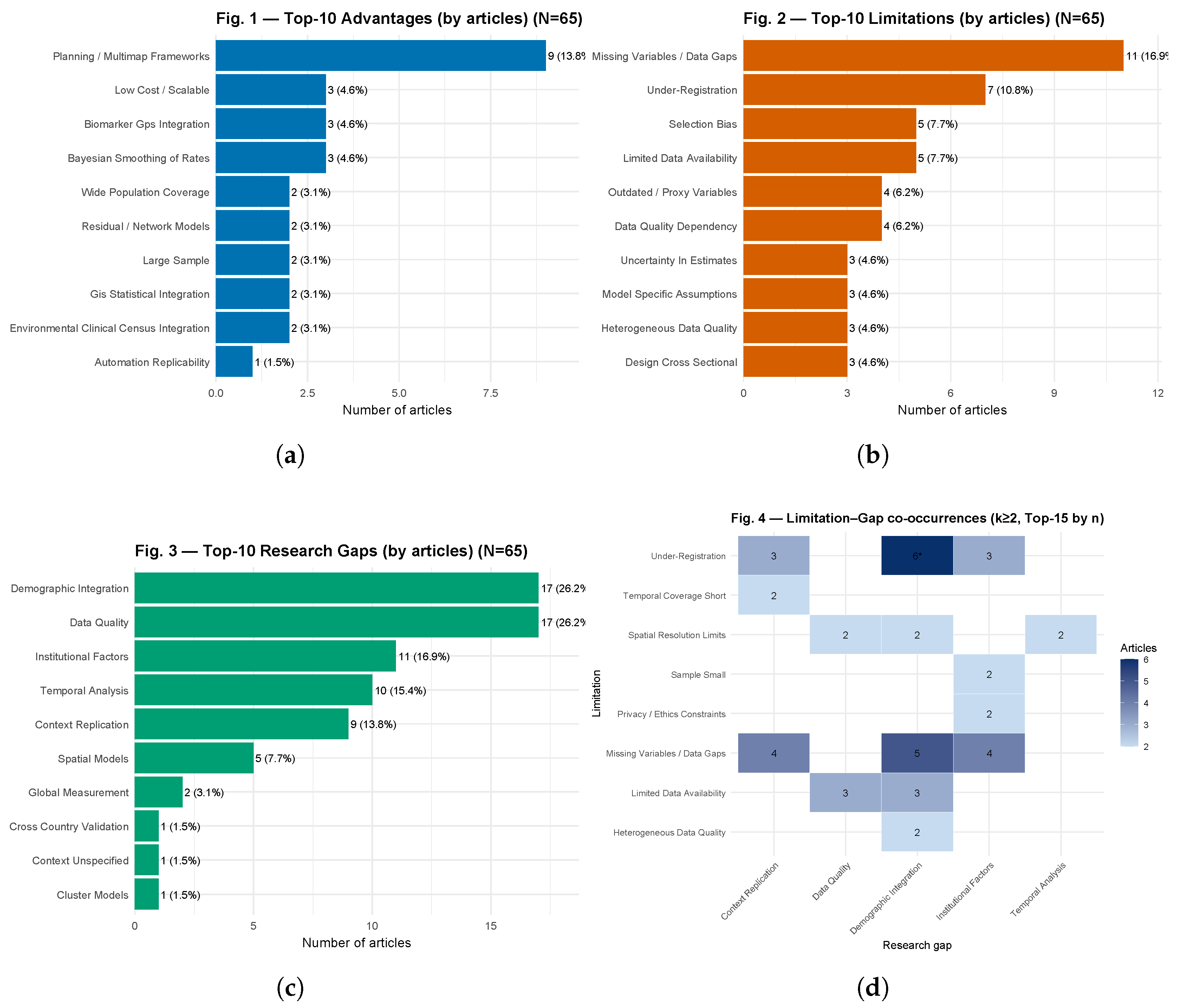
To answer the guiding question, we proceed as follows: Figure 13a outlines the methodological strengths; Figure 13b synthesizes the recurring limitations; Figure 13c elevates these to field-level research needs; and Figure 13d with Table 15 operationalizes the links between limitations and gaps through article-level co-occurrences (), effect sizes, and BH-adjusted evidence, producing a coherent path from data to implications.
The Figure 13a quantifies methodological strengths reported in the corpus (), setting a baseline to interpret subsequent results. In particular, Planning / Multimap Frameworks appears in 9/65 studies (13.8%), while recurrent advantages at 3/65 (4.6%) include Bayesian Smoothing of Rates, Biomarker–GPS Integration, and Low Cost / Scalable. A further set at 2/65 (3.1%)—Environmental–Clinical–Census Integration, GIS–Statistical Integration, Large Sample, National Coverage, and Residual / Network Models—plus one instance at 1/65 (1.5%, Automation / Replicability) collectively point to standardized pipelines, multi-source integration, and stabilized small-area estimates (e.g., via Bayesian smoothing). This baseline previews mechanisms for replicability (traceable procedures) and validity (internal and external) that are contrasted below against limitations and gaps.
Second, Figure 13b identifies bottlenecks that can counteract those strengths and thus guide interpretation: Missing variables / data gaps (11/65; 16.9%) and Under-registration (7/65; 10.8%) top the list, followed by Limited data availability and Selection bias (5/65; 7.7% each), Data quality dependency and Outdated / proxy variables (4/65; 6.2%), and four items at 3/65 (4.6%): Data quality heterogeneous, Uncertainty estimates, Cross-sectional design, and Model-specific assumptions. Accordingly, incompleteness and under-registration threaten internal validity (measurement error/selection bias) and hinder reproduction; at the same time, scarcity and source bias constrain external validity and cross-context generalization.
Third, to translate these risks into actionable needs, Figure 13c prioritizes research gaps: Data Quality and Demographic Integration lead with 17/65 (26.2%) each, followed by Institutional Factors (11/65; 16.9%), Temporal Analysis (10/65; 15.4%), Context Replication (9/65; 13.8%), Spatial Models (5/65; 7.7%), and targeted gaps at 1–2/65 (1.5–3.1%). Consequently, it is most urgent to standardize data quality and metadata, implement reproducible demographic linkage, make institutional constraints transparent, and strengthen spatial and spatiotemporal modelling.
Finally, Figure 13a–d, together with Table 15, operationalize the link between weaknesses and needs by reporting Limitation–Gap co-occurrences () together with effect sizes and evidence. Notably, three pairs show (4.6%): Under-Registration→Institutional Factors (lift , , , ; IDs: [37,58,61]), Limited Data Availability→Data Quality (lift , , , ; IDs: [25,30,53]), and Limited Data Availability→Demographic Integration (same metrics; IDs: [25,55,61]). In addition, two (3.1%) signals exhibit high enrichment—Privacy / Ethics Constraints→Institutional Factors (lift , , , ; IDs: [24,66]) and Sample Small→Institutional Factors (same metrics; IDs: [59,66])—which remain exploratory due to lower support. No Top-10 pair meets (BH), so we treat them as auditable hypotheses; article IDs are listed directly in the table for full traceability. Statistical note for Table ??. For each Limitation–Gap pair, a table over the article universe is formed with counts a (both), b (limitation only), c (gap only), d (neither), with . Columns report , , the enrichment
and the binary effect size
Two-sided Fisher tests are used for inference; multiplicity is controlled with Benjamini–Hochberg to obtain . In exploratory screening we flag as “robust” pairs with and ; otherwise, results should be interpreted cautiously and validated with additional evidence.
Together, (i) Figure 13a profiles reported strengths; (ii) Figure 13b pinpoints recurrent bottlenecks; (iii) Figure 13c elevates these into field-level needs; and (iv) Figure 13d with Table 15 empirically link limitations to gaps through article-level co-occurrences with effect sizes and BH-adjusted evidence—providing a traceable path from data →implications→ actions.
Figure 13.
(a) Top-10 Advantages: most frequent methodological/operational strengths in GIS-based health and citizen-security studies; bars show article counts with percent of the corpus (). (b) Top-10 Limitations: counts with percents; missing variables/data gaps and under-registration dominate, followed by limited data availability and source bias—drivers of lower replicability and external validity. (c) Top-10 Research Gaps: demographic integration and data quality lead, then institutional factors and context replication—priority areas to improve reproducibility and validity. (d) Limitation–Gap co-occurrences (, Top-15 by n): heatmap of limitation (y) vs. gap (x); cell labels are article counts; an asterisk denotes BH-adjusted .
4.3. Integrated Synthesis (SM + SR)
The integrated synthesis connects the descriptive patterns identified through the SM with the quantitative findings derived from the SR. This cross-layer perspective reveals how global production trends and geographical concentrations are linked to specific methodological practices and outcomes, such as accessibility analysis, spatial autocorrelation, and predictive risk modeling. The comparative analysis further highlights relationships between thematic domains, application scenarios, technical parameters, and measurable outcomes, providing a coherent picture of both methodological strengths and persistent gaps. In practical terms, this integration consolidates evidence on accessibility inequities, epidemiological surveillance, and crime reduction, thereby reinforcing the translational value of GIS-based research for evidence-informed public health and urban security policies.
5. Discussion
This study represents the first systematic synthesis that jointly integrates SM and SR of GIS applications in the domains of health and urban security. The findings reveal a methodological ecosystem concentrated on accessibility metrics, spatial autocorrelation, and cluster detection, with a strong geographical bias toward Asia and North America. This concentration demonstrates both the consolidation of GIS as strategic analytical tools and the persistent underrepresentation of highly vulnerable regions where data availability and quality remain uneven.
From a methodological standpoint, this work extends the application of the PRISMA, PICOS, and SPICE frameworks by incorporating quality and reproducibility filters that reinforce evidence traceability [10,11]. The analytical pipeline (7,106 → 65 articles) and the scoring matrix (1–4) provide a transparent and replicable pathway for future geospatial reviews. However, the dominance of cross-sectional observational designs and the limited use of advanced models—such as Bayesian inference, machine learning, or hybrid approaches—confirm persistent methodological gaps within the field.
At an applied level, the results underscore the potential of GIS to assess health inequalities and to inform evidence-based urban security policies. The high spatial resolution and modeling versatility of GIS confirm their suitability for territorial planning and public-policy design. Nevertheless, technological dependency on proprietary platforms (ArcGIS, QGIS) and the coexistence between open datasets—such as DHS, IBGE, or WorldPop—and institutionally restricted databases continue to constrain full replicability and scientific equity. Addressing these challenges requires regulatory frameworks that promote interoperability, data openness, and standardized protocols for spatial validation.
Looking forward, advancing the field will require the opening of multisectoral data sources, the adoption of computationally efficient models suitable for resource-limited environments, and the integration of GIS within reproducible ecosystems combining artificial intelligence and high-performance computing (HPC). Such integration will strengthen transparency, methodological comparability, and the long-term societal impact of geospatial science.
6. Conclusions
The results of this study confirm that GIS have consolidated as strategic analytical tools for addressing public health and urban security challenges, although their application remains characterized by significant geographical and thematic inequalities. Research output is heavily concentrated in Asia and North America, whereas Africa and South America remain underrepresented. This territorial imbalance limits the generalizability of evidence and highlights the need to strengthen research capacities in vulnerable regions.
Methodologically, the fused SM+SR pipeline applied in this study combined the PICOS (health) and SPICE (security) frameworks, systematically filtering an initial corpus of 7,106 references down to 65 core articles. This structured process enhanced reproducibility and enabled the differentiation between robust and weak methodological contributions.
The analysis identified a predominance of cross-sectional observational designs and a methodological core centered on accessibility and spatial autocorrelation indicators. While these approaches offer comparability across contexts, the limited adoption of advanced models—such as Bayesian inference, machine learning, and hybrid AI–GIS pipelines—constrains predictive and causal insights.
The software ecosystem remains highly dependent on ArcGIS and QGIS, complemented by emerging open-source environments such as R, Python, and SaTScan. This configuration promotes standardization but raises concerns about technological dependency and uneven access to computational resources. Expanding interoperability and promoting open geospatial infrastructures are therefore essential steps toward greater scientific equity.
From a scientific standpoint, the most consistent strengths observed across studies include high spatial and temporal resolution, scalability, and multivariate precision. Conversely, key limitations involve the scarcity of openly available data, the predominance of static designs, and the absence of reproducible validation protocols. Addressing these gaps requires methodological standardization, multisource data integration, and computationally efficient modeling suited for resource-limited settings.
In summary, this fused SM+SR framework provides a transparent, replicable, and scalable foundation for synthesizing GIS-based evidence in health and urban security. Advancing toward open data, reproducible validation workflows, and spatially explicit artificial intelligence will be critical to enhancing predictive capacity and policy relevance—particularly in high-vulnerability regions where GIS can directly inform equitable and data-driven decision-making.
Author Contributions
Conceptualization, W.R.M. and I.M.G.; methodology, W.R.M. and V.D.T.; validation, W.R.M., I.M.G. and V.D.T.; formal analysis, W.R.M.; investigation, I.M.G. and V.D.T.; resources, V.D.T. and L.G.G.; data curation, I.M.G. and V.D.T.; writing—original draft preparation, W.R.M. and E.E.G.; writing—review and editing, W.R.M. and E.E.G.; visualization, I.M.G. and E.E.G.; supervision, L.G.G.; project administration, L.G.G.; funding acquisition, L.G.G. All authors have read and agreed to the published version of the manuscript.
Funding
This research received no external funding.
Conflicts of Interest
The authors declare no conflicts of interest.
Abbreviations
The following abbreviations are used in this manuscript:
| GIS | Geographic Information Systems |
| HS | Health-related macro-areas |
| SC | Security-related subdomains |
| SM | Systematic Mapping |
| SR | Systematic Review |
| RQ | Research Question |
| PRISMA | Preferred Reporting Items for Systematic Reviews and Meta-Analyses |
References
- Astuti, E.P.; Dhewantara, P.W.; Prasetyowati, H.; Ipa, M.; Herawati, C.; Hendrayana, K. Paediatric dengue infection in Cirebon, Indonesia: A temporal and spatial analysis of notified dengue incidence to inform surveillance. Parasit Vectors 2019, 12(1), 186. [CrossRef]
- Han, B.; Hu, W.; Tang, X.; Zheng, J.; Hu, M.; Li, Z. Optimization of pre-hospital emergency facility layout in Nanjing: A spatiotemporal analysis using multi-source big data. International Journal of Applied Earth Observation and Geoinformation 2024, 133. [CrossRef]
- Wei, P.; Xie, S.; Huang, L.; Liu, L.; Cui, L.; Tang, Y.; Zhang, Y.; Meng, C.; Zhang, L. Spatial interpolation of regional PM(2.5) concentrations in China during COVID-19 incorporating multivariate data. Atmos Pollut Res 2023, 14(3), 101688. [CrossRef]
- Kendagannaswamy, M.S.; Roopa, C.K.; Harish, B.S.; Mukesh, M.S. Multi-criteria decision analysis for regional-scale flood susceptibility mapping in Kerala State, India. Discover Appl. Sci. 2025, 7, 598. [CrossRef] . [CrossRef]
- Kobayashi, T.; Yamada, K.; Murakami, M.; Ozaki, A.; Torii, H.A.; Uno, K. Assessment of attitudes toward critical actors during public health crises. International Journal of Disaster Risk Reduction 2024, 108. [CrossRef]
- Bediroglu, G.; Colak, H.E. Analysis and visualization of crime data using GIS technology: Understanding crime patterns and distribution. Journal of Geodesy and Geoinformation 2023, 10(2), 151–163. [CrossRef]
- Mishra, P.S.; Kumar, P.; Srivastava, S. Regional inequality in the Janani Suraksha Yojana coverage in India: A geo-spatial analysis. Int J Equity Health 2021, 20(1), 24. [CrossRef]
- Asi, Y.; Mills, D.; Greenough, P.G.; Kunichoff, D.; Khan, S.; van den Hoek, J.; Scher, C.; Halabi, S.; Abdulrahim, S.; Bahour, N.; Ahmed, A.K.; Wispelwey, B.; Hammoudeh, W. ‘Nowhere and no one is safe’: Spatial analysis of damage to critical civilian infrastructure in the Gaza Strip during the first phase of the Israeli military campaign, 7 October to 22 November 2023. Confl Health 2024, 18(1), 24. [CrossRef]
- Nunes, P.S.; Guimaraes, R.A.; Martelli, C.M.T.; de Souza, W.V.; Turchi, M.D. Zika virus infection and microcephaly: Spatial analysis and socio-environmental determinants in a region of high Aedes aegypti infestation in the Central-West Region of Brazil. BMC Infect Dis 2021, 21(1), 1107. [CrossRef]
- Carrasco, K.; Tomalá, L.; Ramírez Meza, E.; Meza Bolaños, D.; Ramírez Montalván, W. Computational Techniques in PET/CT Image Processing for Breast Cancer: A Systematic Mapping Review. ACM Comput. Surv. 2024, 56(8), 197 (38 pp.). [CrossRef]
- Ramírez, W.; Pillajo, V.; Ramírez, E.; Manzano, I.; Meza, D. Exploring Components, Sensors, and Techniques for Cancer Detection via eNose Technology: A Systematic Review. Sensors 2024, 24(23), 7868. [CrossRef]
- Central Statistical Agency (CSA) [Ethiopia]; ICF. Ethiopia Demographic and Health Survey 2016; CSA and ICF: Addis Ababa, Ethiopia, 2017. Available online: http://dhsprogram.com/pubs/pdf/FR328/FR328.pdf.
- International Institute for Population Sciences (IIPS) [India]; ICF. National Family Health Survey (NFHS-5), 2019–21: India: Volume I; IIPS: Mumbai, India, 2022. Available online: https://www.dhsprogram.com/pubs/pdf/FR375/FR375.pdf.
- Uganda Bureau of Statistics (UBOS); ICF. Uganda Demographic and Health Survey 2016; UBOS and ICF: Kampala, Uganda, 2018. Available online: http://dhsprogram.com/pubs/pdf/FR333/FR333.pdf.
- National Institute of Statistics (Cameroon); ICF. 2018 Cameroon DHS Summary Report; NIS and ICF: Rockville, MD, USA, 2020. Available online: https://dhsprogram.com/pubs/pdf/SR266/SR266.pdf.
- Instituto Brasileiro de Geografia e Estatística (IBGE). Sinopse do Censo Demográfico: 2010; IBGE: Rio de Janeiro, Brazil, 2011; 265 p.; ISBN 9788524041877. Available online: https://biblioteca.ibge.gov.br/visualizacao/livros/liv49230.pdf.
- WorldPop (School of Geography and Environmental Science, University of Southampton); Department of Geography and Geosciences, University of Louisville; Département de Géographie, Université de Namur; Center for International Earth Science Information Network (CIESIN), Columbia University. Global High Resolution Population Denominators Project—Funded by The Bill and Melinda Gates Foundation (OPP1134076). Dataset 2018. [CrossRef]
- Kianfar, N.; Mesgari, M.S. GIS-based spatio-temporal analysis and modeling of COVID-19 incidence rates in Europe. Spat Spatiotemporal Epidemiol 2022, 41, 100498. [CrossRef]
- Marcelo-Diaz, C.; Lesmes, M.C.; Santamaria, E.; Salamanca, J.A.; Fuya, P.; Cadena, H.; Munoz-Laiton, P.; Morales, C.A. Spatial analysis of dengue clusters at department, municipality and local scales in the Southwest of Colombia, 2014–2019. Trop Med Infect Dis 2023, 8, 262. [CrossRef]
- Shoaib, M.; Ullah, A.; Abbasi, I.A.; Algarni, F.; Khan, A.S. Augmenting the robustness and efficiency of violence detection systems for surveillance and non-surveillance scenarios. IEEE Access 2023, 11, 123295–123313. [CrossRef]
- Sritart, H.; Miyazaki, H.; Kanbara, S.; Taertulakarn, S. Geospatial patterns of property crime in Thailand: A socioeconomic perspective for sustainable cities. Sustainability 2025, 17(14). [CrossRef]
- Gordan, M.; Kountche, D.A.; McCrum, D.; Schauer, S.; König, S.; Delannoy, S.; Connolly, L.; Iacob, M.; Durante, N.G.; Shekhawat, Y.; Carrasco, C.; Katsoulakos, T.; Carroll, P. Protecting critical infrastructure against cascading effects: The PRECINCT approach. Resilient Cities and Structures 2024, 3(3), 1–19. [CrossRef]
- Belay, A.S.; Sarma, H.; Yilak, G. Spatial distribution and determinants of unmet need for family planning among all reproductive-age women in Uganda: A multi-level logistic regression modeling approach and spatial analysis. Contracept Reprod Med 2024, 9(1), 4. [CrossRef]
- Chen, X.; Chen, B.; Zhang, H.; Wong, C.U.I. Research on the spatial and temporal distribution evolution and sustainable development mechanism of smart health and elderly care demonstration bases based on GIS. Applied Sciences 2024, 14(2). [CrossRef]
- Pesaresi, C.; Pavia, D.; De Vito, C.; Barbara, A.; Cerabona, V.; Di Rosa, E. Dynamic space-time diffusion simulator in a GIS environment to tackle the COVID-19 emergency: Testing a geotechnological application in Rome. Geographia Technica 2021(Special Issue), 82–99. [CrossRef]
- Yongheng, D.; Shan, X.; Fei, L.; Jinglin, T.; Liyue, G.; Xiaoying, L.; Tingxiao, W.; Hongrui, W. GIS-based assessment of spatial and temporal disparities of urban health index in Shenzhen, China. Front Public Health 2024, 12, 1429143. [CrossRef]
- Parandin, F.; et al. Risk mapping and spatial modeling of human cystic echinococcosis in Iran from 2009 to 2018: A GIS-based survey. Iran. J. Parasitol. 2022, 17(3), 306–316. [CrossRef] . [CrossRef]
- Alamneh, T.S.; Teshale, A.B.; Yeshaw, Y.; Alem, A.Z.; Ayalew, H.G.; Liyew, A.M.; Tessema, Z.T.; Tesema, G.A.; Worku, M.G. Barriers for health care access affect maternal continuum of care utilization in Ethiopia: Spatial analysis and generalized estimating equation. PLoS ONE 2022, 17(4), e0266490. [CrossRef] . [CrossRef]
- Brown-Amilian, S.; Akolade, Y. Disparities in COPD hospitalizations: A spatial analysis of proximity to toxics release inventory facilities in Illinois. Int J Environ Res Public Health 2021, 18(24). [CrossRef]
- Das, S.; Bikram, P.; Biswas, A.; C, V.; Sinha, P. Multilayer optimized deep learning model to analyze spectral indices for predicting the condition of rice blast disease. Remote Sensing Applications: Society and Environment 2025, 37. [CrossRef]
- Gausman, J.; Pingray, V.; Adanu, R.; Bandoh, D.A.B.; Berrueta, M.; Blossom, J.; Chakraborty, S.; Dotse-Gborgbortsi, W.; Kenu, E.; Khan, N.; Langer, A.; Nigri, C.; Odikro, M.A.; Ramesh, S.; Saggurti, N.; Vazquez, P.; Williams, C.R.; Jolivet, R.R. Validating indicators for monitoring availability and geographic distribution of emergency obstetric and newborn care (EmoNC) facilities: A study triangulating health system, facility, and geospatial data. PLoS One 2023, 18(9), e0287904. [CrossRef]
- Lardier, D.T., Jr.; Blackwell, M.A.; Beene, D.; Lin, Y. Social vulnerabilities and spatial access to primary healthcare through car and public transportation system in the Albuquerque, NM, Metropolitan Area: Assessing disparities through GIS and multilevel modeling. J Urban Health 2023, 100(1), 88–102. [CrossRef]
- Mollalo, A.; Mao, L.; Rashidi, P.; Glass, G.E. A GIS-based artificial neural network model for spatial distribution of tuberculosis across the continental United States. Int J Environ Res Public Health 2019, 16(1). [CrossRef]
- Naboureh, A.; Feizizadeh, B.; Naboureh, A.; Bian, J.; Blaschke, T.; Ghorbanzadeh, O.; Moharrami, M. Traffic accident spatial simulation modeling for planning of road emergency services. ISPRS Int. J. Geo-Inf. 2019, 8(9). [CrossRef]
- Sandie, A.B.; Tchatchueng Mbougua, J.B.; Nlend, A.E.N.; Thiam, S.; Nono, B.F.; Fall, N.A.; Senghor, D.B.; Sylla, E.H.M.; Faye, C.M. Hot-spots of HIV infection in Cameroon: A spatial analysis based on Demographic and Health Surveys data. BMC Infect Dis 2022, 22(1), 334. [CrossRef]
- Scott, L.E.; Shapiro, A.N.; Da Silva, M.P.; Tsoka, J.; Jacobson, K.R.; Emch, M.; Moultrie, H.; Jenkins, H.E.; Moore, D.; Van Rie, A.; Stevens, W.S. Integrating molecular diagnostics and GIS mapping: A multidisciplinary approach to understanding tuberculosis disease dynamics in South Africa using Xpert MTB/RIF. Diagnostics (Basel) 2023, 13(20). [CrossRef]
- Tan, L.M.; Hung, D.N.; My, D.T.; Walker, M.A.; Ha, H.T.T.; Thai, P.Q.; Hung, T.T.M.; Blackburn, J.K. Spatial analysis of human and livestock anthrax in Dien Bien province, Vietnam (2010–2019) and the significance of anthrax vaccination in livestock. PLoS Negl Trop Dis 2022, 16(12), e0010942. [CrossRef]
- Tilahun, W.M.; Tesfie, T.K. Spatial variation of premarital HIV testing and its associated factors among married women in Ethiopia: Multilevel and spatial analysis using 2016 demographic and health survey data. PLoS One 2023, 18(11), e0293227. [CrossRef]
- Weliange, S.S.; Fernando, D.; Withanage, S.; Gunatilake, J. A GIS based approach to neighbourhood physical environment and walking among adults in Colombo municipal council area, Sri Lanka. BMC Public Health 2021, 21(1), 989. [CrossRef]
- Yang, Q.; Liu, G.; Gonella, F.; Chen, Y.; Liu, C.; Zhao, H.; Yang, Z. Assessing the temporal–spatial dynamic reduction in ecosystem services caused by air pollution: A near-real-time data perspective. Resources, Conservation and Recycling 2022, 180. [CrossRef]
- Wang, S.; Ren, Z. Spatial variations and macroeconomic determinants of life expectancy and mortality rate in China: A county-level study based on spatial analysis models. Int J Public Health 2019, 64(5), 773–783. [CrossRef]
- Alsharif, A.T. Georeferencing of Current Dental Service Locations to Population Census Data: Identification of Underserved Areas in Al Madina, Saudi Arabia. SAGE Open 2020, 10(4). [CrossRef]
- Cardoso, D.T.; de Souza, D.C.; de Castro, V.N.; Geiger, S.M.; Barbosa, D.S. Identification of priority areas for surveillance of cutaneous leishmaniasis using spatial analysis approaches in Southeastern Brazil. BMC Infect Dis 2019, 19(1), 318. [CrossRef]
- Ghazvini, A.; Abdullah, S.N.H.S.; Hasan, M.K.; Bin Kasim, D.Z.A. Crime spatiotemporal prediction with fused objective function in time delay neural network. IEEE Access 2020, 8, 115167–115183. [CrossRef]
- Schultes, O.L.; Morais, M.H.F.; Cunha, M.; Sobral, A.; Caiaffa, W.T. Spatial analysis of dengue incidence and Aedes aegypti ovitrap surveillance in Belo Horizonte, Brazil. Trop Med Int Health 2021, 26(2), 237–255. [CrossRef]
- Zaidi, S.M.A.; Jamal, W.Z.; Mergenthaler, C.; Azeemi, K.S.; Van Den Berge, N.; Creswell, J.; Khan, A.; Khowaja, S.; Habib, S.S. A spatial analysis of TB cases and abnormal X-rays detected through active case-finding in Karachi, Pakistan. Sci Rep 2023, 13(1), 1336. [CrossRef]
- MacPherson, P.; Khundi, M.; Nliwasa, M.; Choko, A.T.; Phiri, V.K.; Webb, E.L.; Dodd, P.J.; Cohen, T.; Harris, R.; Corbett, E.L. Disparities in access to diagnosis and care in Blantyre, Malawi, identified through enhanced tuberculosis surveillance and spatial analysis. BMC Med 2019, 17(1), 21. [CrossRef]
- Rudisill, T.M.; Barbee, L.O.; Hendricks, B. Characteristics of fatal, pedestrian-involved, motor vehicle crashes in West Virginia: A cross-sectional and spatial analysis. Int J Environ Res Public Health 2023, 20(7). [CrossRef]
- Sahat, O.; Kamsa-Ard, S.; Suwannatrai, A.T.; Lim, A.; Kamsa-Ard, S.; Bilheem, S.; Daoprasert, K.; Leklob, A.; Uadrang, S.; Santong, C.; Sriket, N.; Chansaard, W. Spatial analysis of cholangiocarcinoma in Thailand from 2012 to 2021: A population-based cancer registries study. PLoS One 2024, 19(12), e0311035. [CrossRef]
- Baligh Jahromi, A.; Attarian, K.; Asgary, A.; Wu, J. Advancing indoor epidemiological surveillance: Integrating real-time object detection and spatial analysis for precise contact rate analysis and enhanced public health strategies. Int J Environ Res Public Health 2024, 21(11). [CrossRef]
- Cowton, J.; Kyriazakis, I.; Bacardit, J. Automated individual pig localisation, tracking and behaviour metric extraction using deep learning. IEEE Access 2019, 7, 108049–108060. [CrossRef]
- Lin, Y.; Hoover, J.; Beene, D.; Erdei, E.; Liu, Z. Environmental risk mapping of potential abandoned uranium mine contamination on the Navajo Nation, USA, using a GIS-based multi-criteria decision analysis approach. Environ Sci Pollut Res Int 2020, 27(24), 30542–30557. [CrossRef]
- Umair, A.; Masciari, E. Sentimental and spatial analysis of COVID-19 vaccines tweets. J Intell Inf Syst 2023, 60(1), 1–21. [CrossRef]
- Vurro, F.; Croci, M.; Impollonia, G.; Marchetti, E.; Gracia-Romero, A.; Bettelli, M.; Araus, J.L.; Amaducci, S.; Janni, M. Field plant monitoring from macro to micro scale: Feasibility and validation of combined field monitoring approaches from remote to in vivo to cope with drought stress in tomato. Plants 2023, 12(22), 3851. [CrossRef] . [CrossRef]
- Bauer, J.; Bruggmann, D.; Klingelhofer, D.; Maier, W.; Schwettmann, L.; Weiss, D.J.; Groneberg, D.A. Access to intensive care in 14 European countries: A spatial analysis of intensive care need and capacity in the light of COVID-19. Intensive Care Med 2020, 46(11), 2026–2034. [CrossRef]
- Dessie, A.M.; Zemene, M.A.; Gebeyehu, A.A.; Gebeyehu, N.A.; Adella, G.A.; Kassie, G.A.; Mengstie, M.A.; Seid, M.A.; Abebe, E.C.; Gesese, M.M.; Kebede, Y.S.; Moges, N.; Bantie, B.; Feleke, S.F.; Dejenie, T.A.; Chanie, E.S.; Bayih, W.A.; Tesfa, N.A.; Aychew, E.W.; Mekuriaw, B.Y.; Anley, D.T. Hotspot areas of tetanus-unprotected births and its associated factors in Ethiopia: Spatial analysis of EDHS data. Hum Vaccin Immunother 2024, 20(1), 2298062. [CrossRef]
- Meher, T.; Sahoo, H. Dynamics of usage of menstrual hygiene and unhygienic methods among young women in India: A spatial analysis. BMC Womens Health 2023, 23(1), 573. [CrossRef]
- San Sebastian, M.; Vives-Cases, C.; Goicolea, I. “Closer to the unfair reality”: Magnitude and spatial analysis of femicides in Ecuador. J Interpers Violence 2021, 36(17–18), NP9982–NP9993. [CrossRef]
- Song, J.; Ok, S.M.; Kwon, E.Y.; Kim, H.J.; Lee, J.Y.; Joo, J.Y. Fatty acid binding protein 4 could be a linking biomarker between periodontitis and systemic diseases. Biomedicines 2025, 13(2). [CrossRef]
- Sun, H.; Wang, A.; He, S. Temporal and spatial analysis of Alzheimer’s disease based on an improved convolutional neural network and a resting-state fMRI brain functional network. Int J Environ Res Public Health 2022, 19(8). [CrossRef]
- Calo, F.D.; Quinco, M.K.C.; Lachica, Z.P.T.; Logrosa, G.T.; Diche, Z.J.I.; Roxas, P.G.J.; Ligue, K.D.B.; Bompat, J.M.A.; Catalan, J.M.G.; Yumang, A.P.; Mata, M.A.E. Retrospective spatial analysis of the COVID-19 threat to the high-risk population in Davao Region, Philippines from March 2020 to August 2021. Philipp. J. Sci. 2023, 152(3), 897–917. https://philjournalsci.dost.gov.ph/images/pdf/pjs_pdf/vol152no3/retrospective_spatial_analysis_covid19.pdf.
- Anwer, S.; Li, H.; Antwi-Afari, M.F.; Umer, W.; Mehmood, I.; Al-Hussein, M.; Wong, A.Y.L. Test–retest reliability, validity, and responsiveness of a textile-based wearable sensor for real-time assessment of physical fatigue in construction bar-benders. Journal of Building Engineering 2021, 44. [CrossRef]
- Kibuuka, D.; Mpofu, C.; Neave, P.; Manda, S. A spatial analysis of tuberculosis related mortality in South Africa. Int J Environ Res Public Health 2021, 18(22). [CrossRef]
- Kundu, S.; Sharma, P.; Singh, S.; Kumar, P. District-level heterogeneity in overweight or obesity among women of reproductive age: A geo-spatial analysis in India. PLoS One 2023, 18(8), e0290020. [CrossRef]
- Tuntun, M.; Aminah, S.; Yusrizal, C.H. Distribution pattern and spatial analysis of factors for tuberculosis (TB) cases in Bandar Lampung City in 2022. Bali Medical Journal 2022, 12(1), 50–58. [CrossRef]
- Vedaei, S.S.; Fotovvat, A.; Mohebbian, M.R.; Rahman, G.M.E.; Wahid, K.A.; Babyn, P.; Marateb, H.R.; Mansourian, M.; Sami, R. COVID-SAFE: An IoT-based system for automated health monitoring and surveillance in post-pandemic life. IEEE Access 2020, 8, 188538–188551. [CrossRef]
- Audi, M.N.; Mwenda, K.M.; Wei, G.; Lurie, M.N. Healthcare accessibility in preconflict Syria: A comparative spatial analysis. BMJ Open 2022, 12(5), e059210. [CrossRef]
- Ramirez-Aldana, R.; Gomez-Verjan, J.C.; Bello-Chavolla, O.Y. Spatial analysis of COVID-19 spread in Iran: Insights into geographical and structural transmission determinants at a province level. PLoS Negl Trop Dis 2020, 14(11), e0008875. [CrossRef]
- Cabrera-Barona, P.F.; Jimenez, G.; Melo, P. Types of crime, poverty, population density and presence of police in the Metropolitan District of Quito. ISPRS Int. J. Geo-Inf. 2019, 8(12). [CrossRef]
- Yu, J.; Leung, M.Y.; Ma, G.; Xia, J. Older adults’ access to and satisfaction with primary hospitals based on spatial and non-spatial analyses. Front Public Health 2022, 10, 845648. [CrossRef]
- Garnica-Monroy, R.; Garibay-Bravo, V.; Gonzalez-Gonzalez, A.; Martínez Salgado, H.; Hernández-Reyes, M. Spatial analysis of exposure to traffic-related air pollution in Mexico: Implications for urban planning to improve public health. Applied Spatial Analysis and Policy 2021, 15(3), 647–665. [CrossRef]
- Maxwell, S.P.; Brooks, C.; Kim, D.; McNeely, C.L.; Cho, S.; Thomas, K.C. Improving surveillance of human tick-borne disease risks: Spatial analysis using multimodal databases. JMIR Public Health Surveill 2023, 9, e43790. [CrossRef]
- Guevara, C.; Penas, M.S. Surveillance routing of COVID-19 infection spread using an intelligent infectious diseases algorithm. IEEE Access 2020, 8, 201925–201936. [CrossRef]
| 1 | |
| 2 | |
| 3 | |
| 4 | |
| 5 | |
| 6 |
Figure 1.
Distribution of articles by year and publisher (GIS + Health + Security). Stacked bar chart (a) showing the annual production of articles aggregated by the six most prolific publishers and grouped as “Others.” Line chart (b) illustrating temporal trends from 2019 to 2025. Data correspond to the systematic mapping dataset (n = 65 articles).
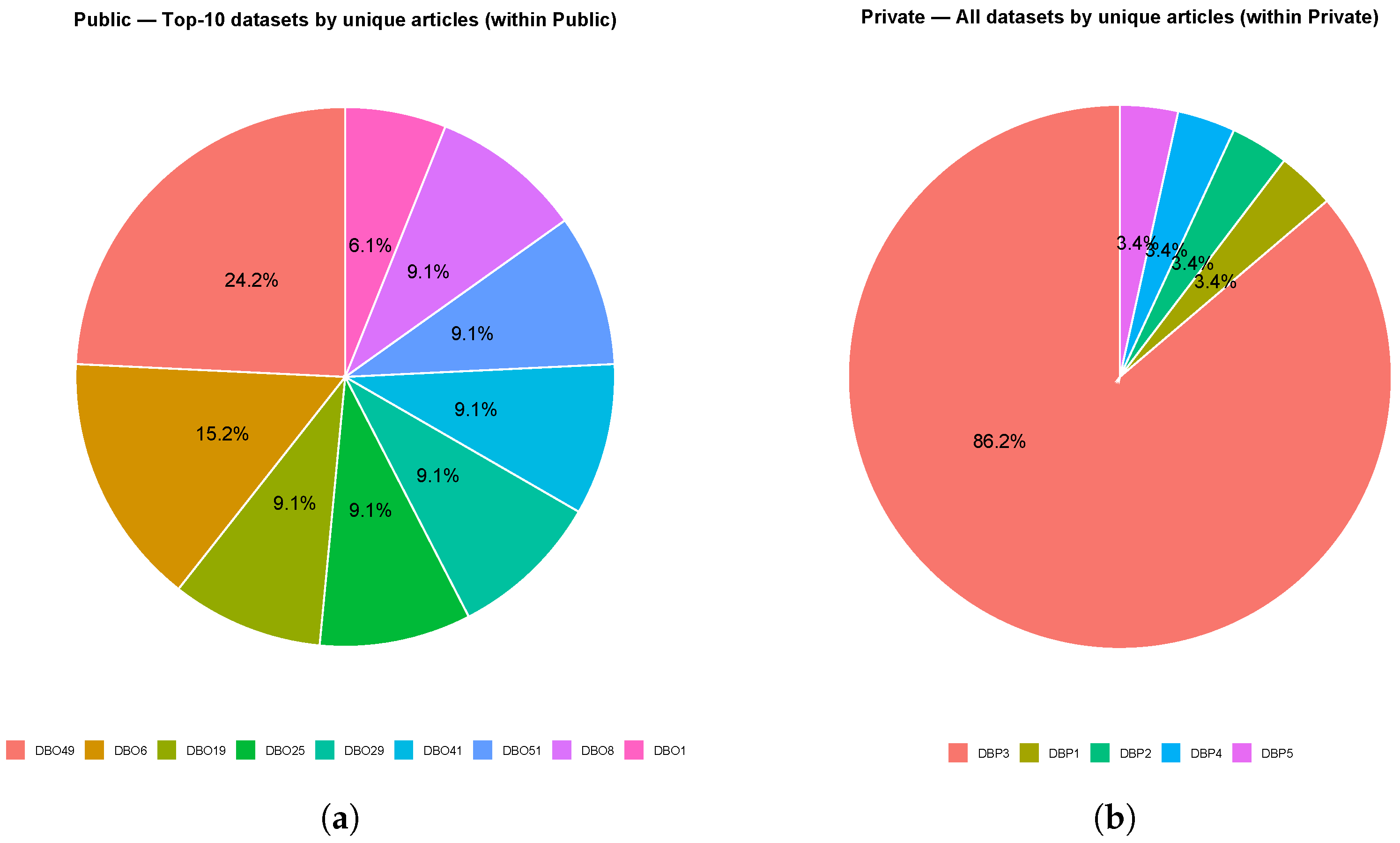
Figure 3.
The regions represent the geographic areas where the study was conducted (variables Geographic Area / Country–Region), and not the institutional affiliation or editorial location. The stacked bars display the annual territorial distribution, while the line indicates the annual percentage relative to the total corpus ().
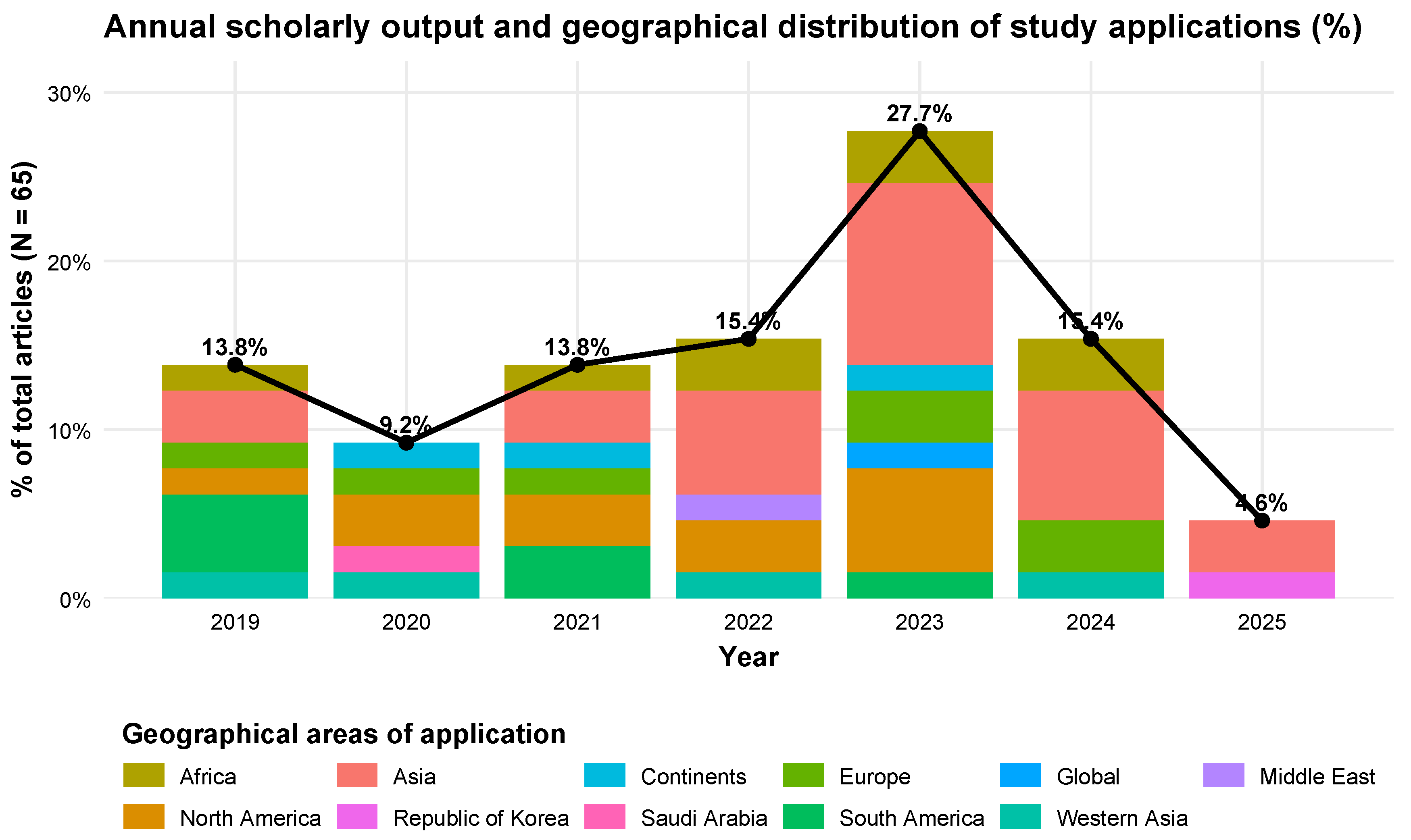
Figure 4.
The cumulative distribution is shown by macro-region (x-axis) and percentage over the total (y-axis), with stacking by domains (Domain = Health / Public Safety). The top label of each bar reports both the absolute count and the percentage per region.
Figure 4.
The cumulative distribution is shown by macro-region (x-axis) and percentage over the total (y-axis), with stacking by domains (Domain = Health / Public Safety). The top label of each bar reports both the absolute count and the percentage per region.
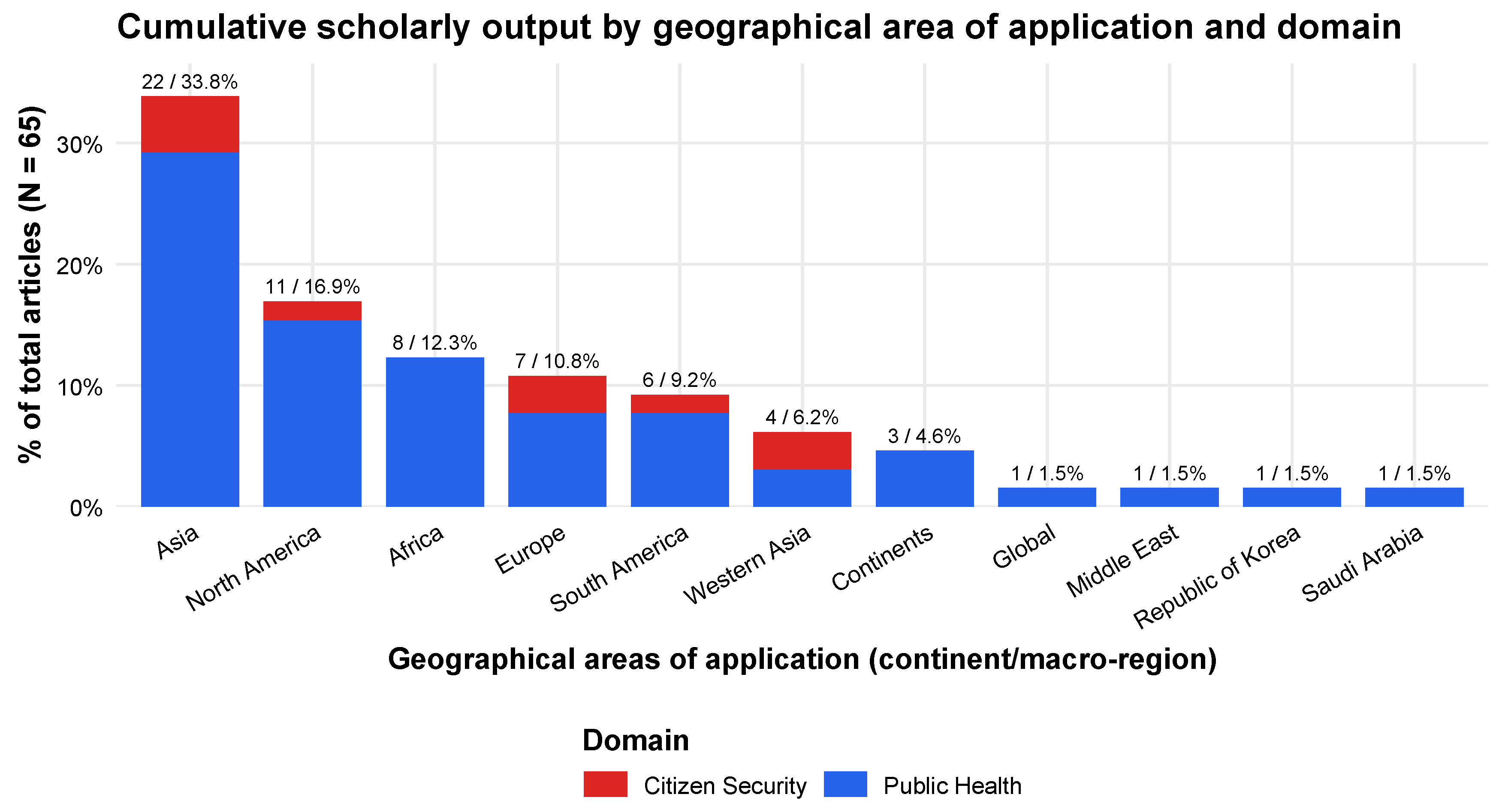
Figure 5.
Distribution of the 65 articles classified into health (HS-) macro-areas and security (SC-) subdomains by application setting. Bars show the number of articles (n) with absolute counts and percentages of the global corpus (N = 65). Health-related studies are mainly situated in national and regional contexts, whereas security-related studies concentrate in urban and subnational/regional contexts.
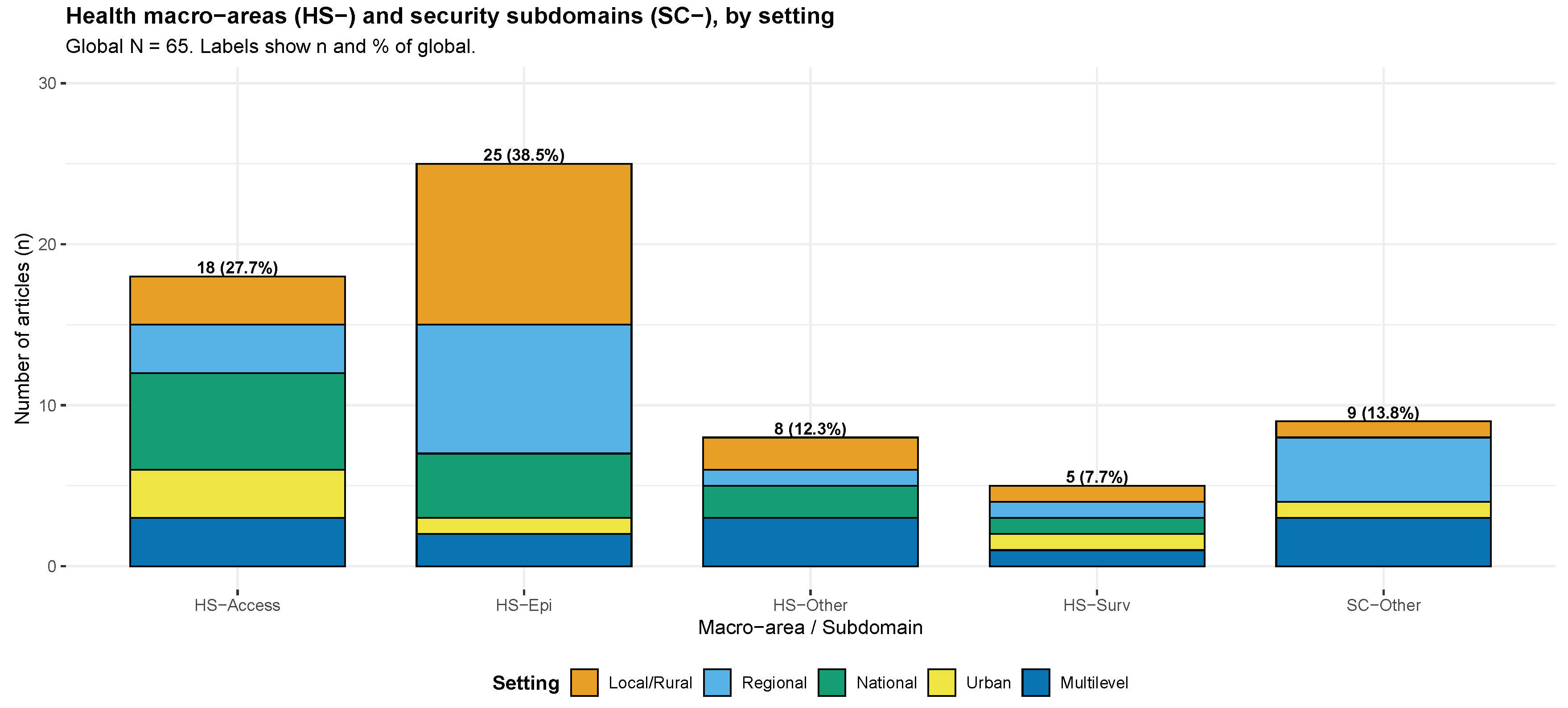
Figure 6.
Study Type × Methodological Design (Pareto). Cumulative coverage of 65 combinations with 95% Wilson confidence intervals. Top-5 categories account for 49.2% of the corpus; diversity indices (HHI = 0.067, Gini = 0.367, Shannonn = 0.926) reflect moderate concentration and methodological diversity.
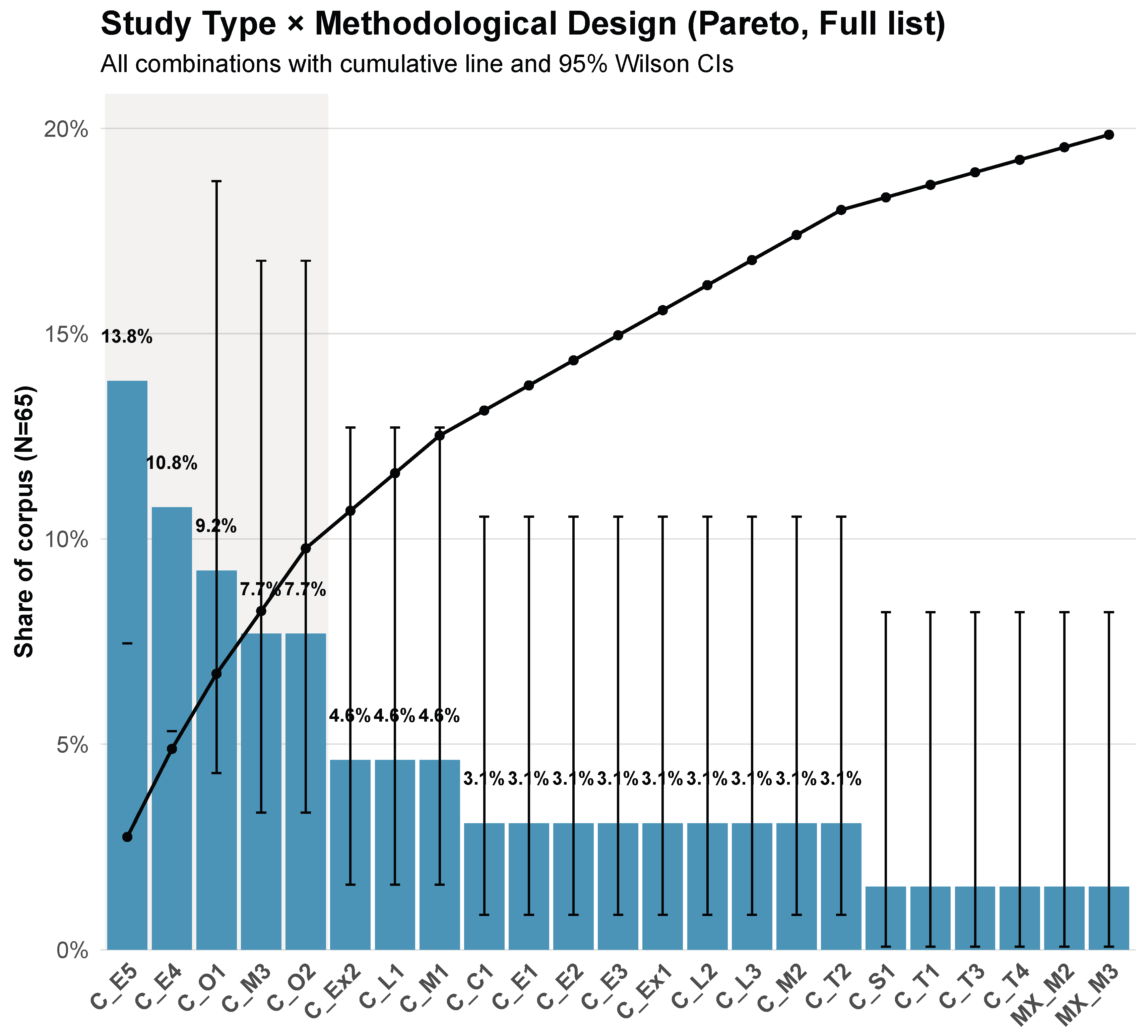
Figure 7.
Distribution of total and core high–impact articles (Q1 & Active JCR) across the top-12 journals. Values above bars indicate absolute counts with global percentages (Total) and internal percentages (Core). Journals are abbreviated J1–J12, see Table 10.
Figure 7.
Distribution of total and core high–impact articles (Q1 & Active JCR) across the top-12 journals. Values above bars indicate absolute counts with global percentages (Total) and internal percentages (Core). Journals are abbreviated J1–J12, see Table 10.
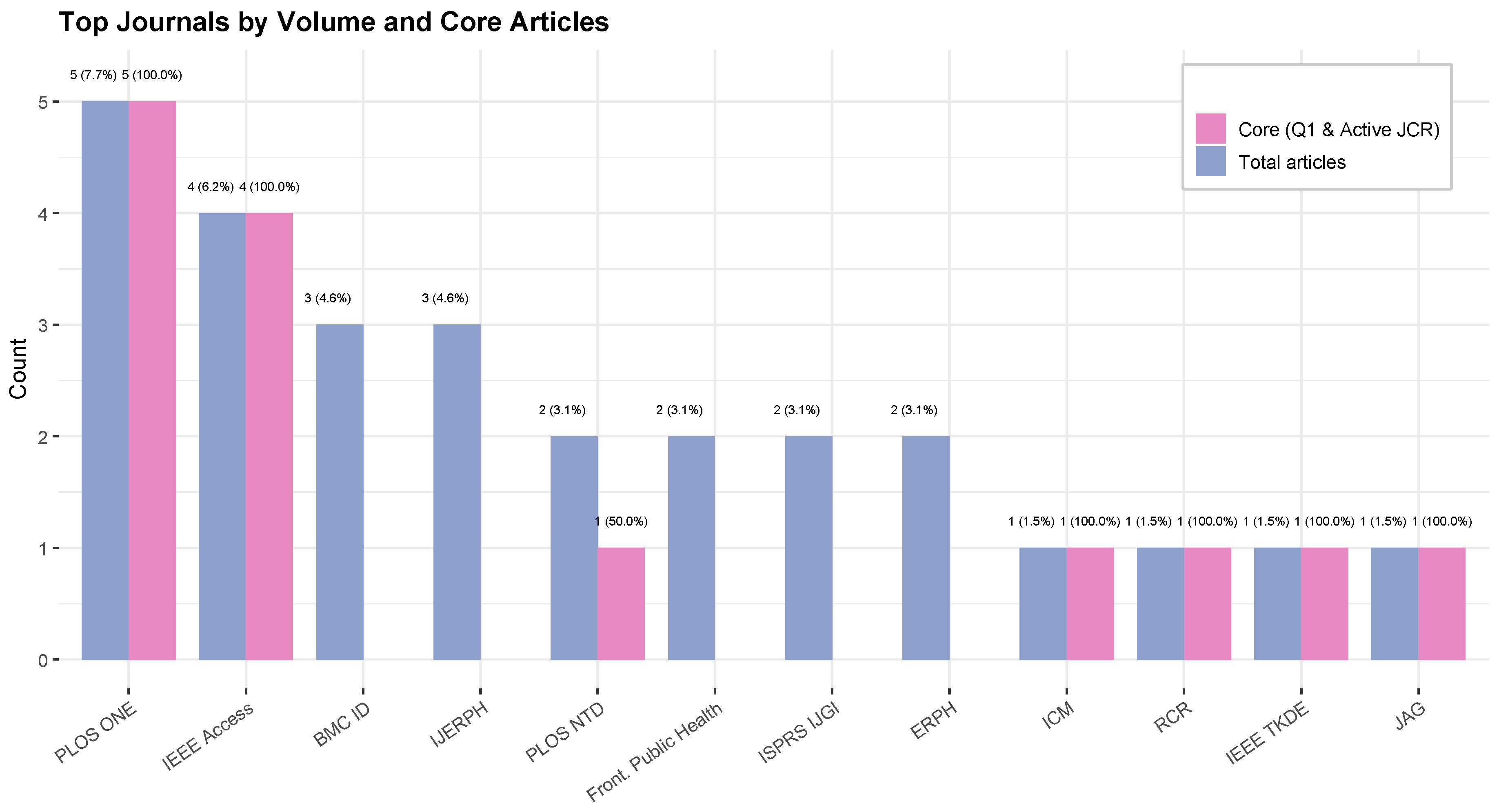
Figure 8.
Distribution of total and core high–impact articles (Q1 & Active JCR) across parent categories. Mean impact factor is indicated by the red line and points (secondary axis). Values above bars indicate absolute counts with global percentages (Total) and internal percentages (Core). Categories are abbreviated C1–Ck, see Table 10.
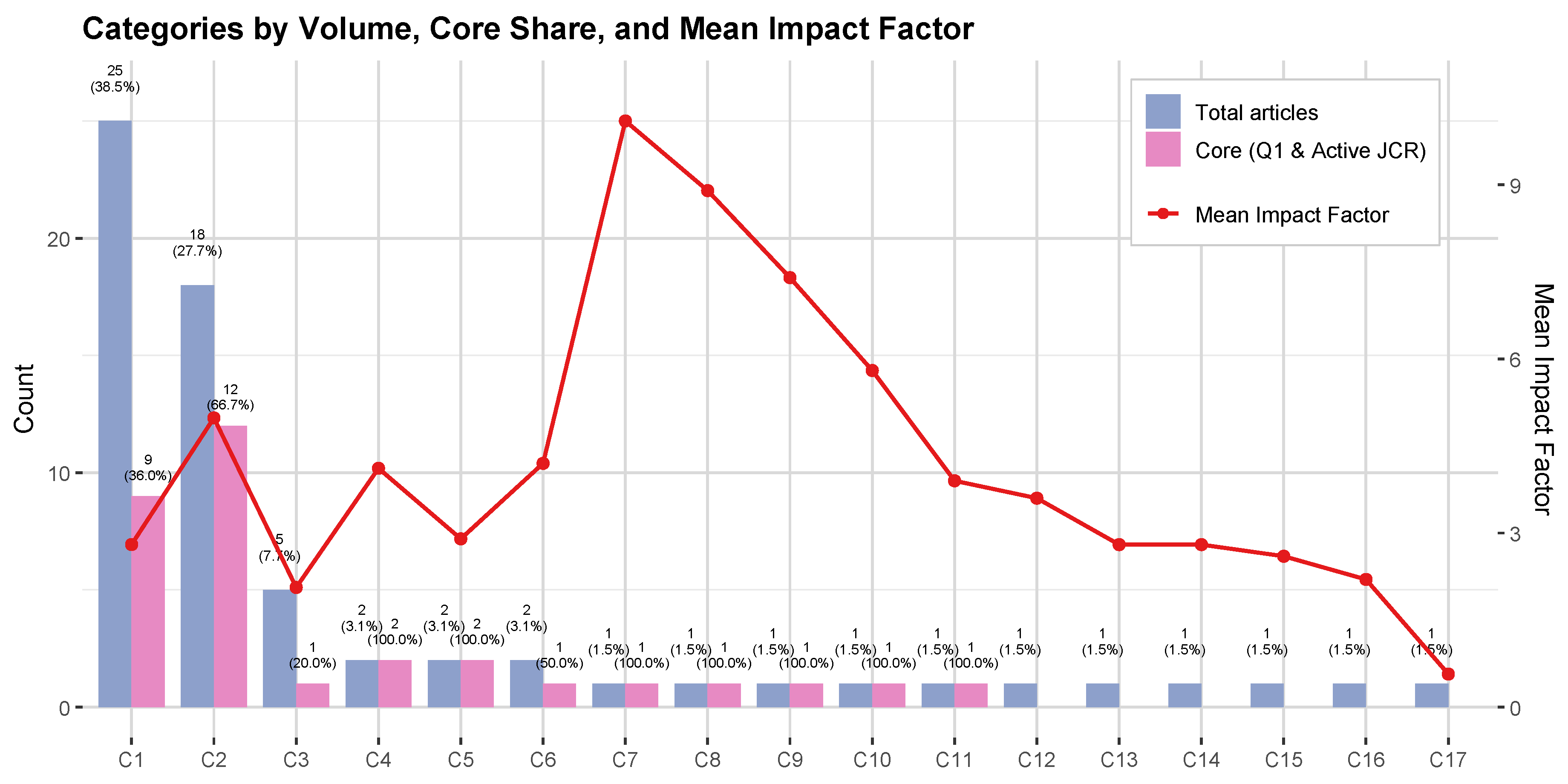
Figure 9.
Pareto chart of the 40 most frequent metrics, stacked by domain (health = red, security = blue). Bars indicate absolute frequencies (N) with cumulative proportion (black line). The top five metrics (MRV, CFF, PRC, CNT, SMTR) cover > 40% and the top ten > 60%, revealing strong methodological concentration and domain asymmetry favoring health.
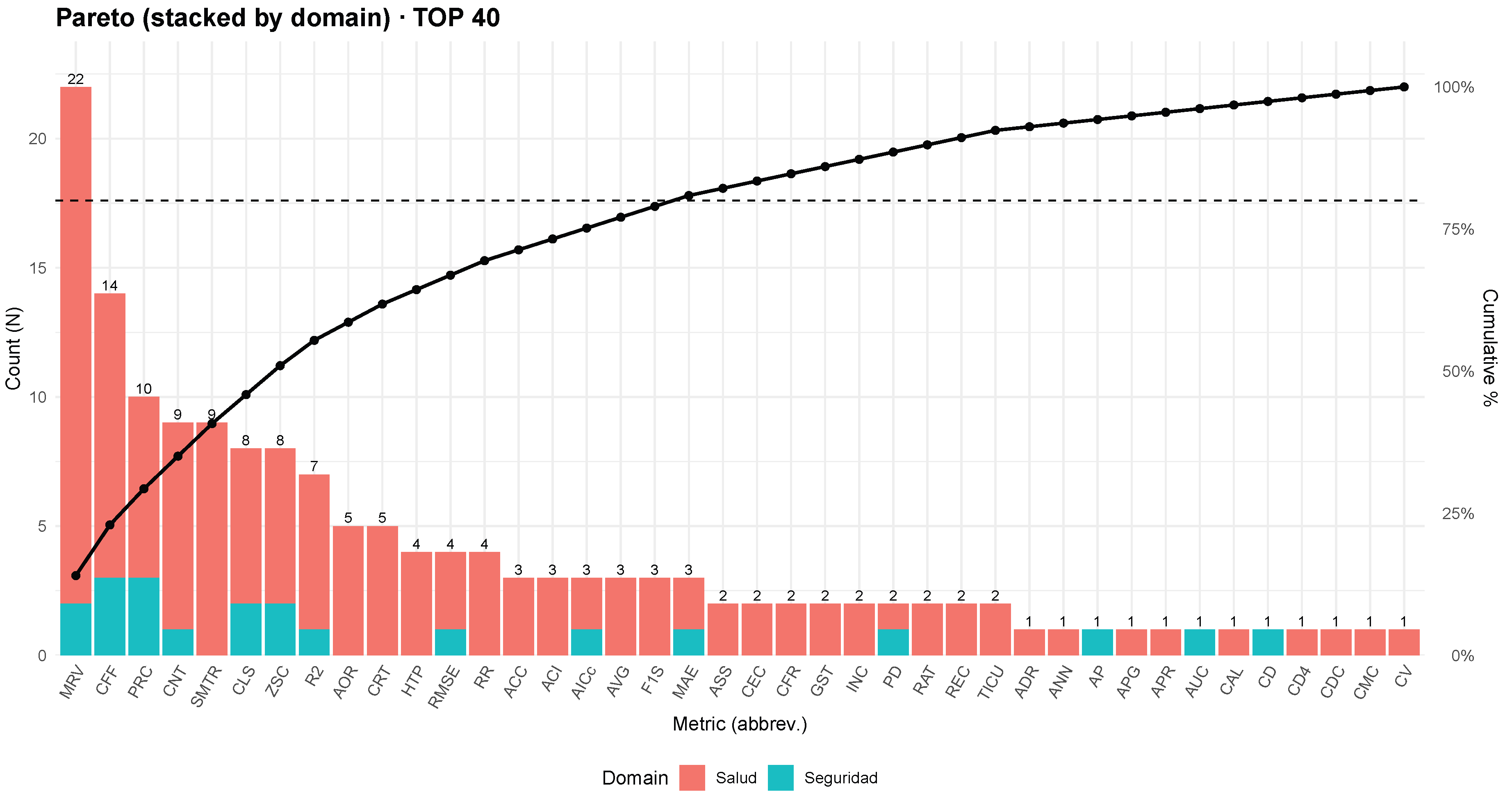
Figure 10.
Distribution of articles by year and publisher (GIS + Health + Security). Stacked bar chart (a) Temporal evolution of the Top-10 metrics with 95% confidence intervals. Lines show, for each period (≤2019, 2020–2021, 2022–2023, ≥2024), the percentage of unique articles reporting each metric. Shaded bands correspond to 95% Wilson binomial confidence intervals, computed with denominator (number of unique articles in that period). (b) Heatmap of Top-10 metrics by period. The color gradient represents the proportion of unique articles using each metric within a given period, normalized by . Darker shades highlight peaks of adoption (e.g., Moran’s I in ≥2024).

Figure 11.
Distribution of the 13 tools and platforms reported across the 65 GIS-based health and public-safety studies. Bars indicate the number of unique articles (n) with 95% Wilson binomial confidence intervals. The black line denotes cumulative coverage, and the dashed vertical line marks the 80% Pareto threshold.

Figure 12.
(a) Effect (Top-20): vertical lollipops of (winsorized at 6); dashed lines at , , . Line color encodes group (green: both; orange: de_punta_only). Symbols: ◯ canonical / □ secondary; solid = both, hollow = de_punta_only. Label “” indicates truncation. (b) Robustness (BOTH): vertical lollipops showing proportion of significant tests (); color and thickness indicate robustness tier (R1 high; R2 moderate; R3 limited). Thin segments show 95% Wilson CIs; dashed line at marks null expectation; labels above points: , † for .
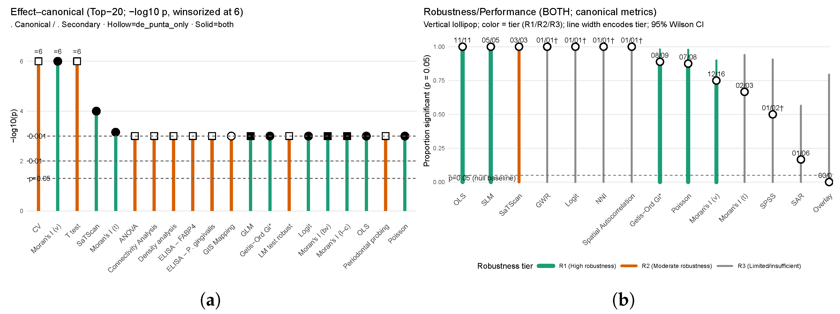
Table 3.
Distribution by publisher across BDB / SM Filters and SR.
| Publisher | BDB1 | SM Filters3 | SR Filters4 | |||||||||
|---|---|---|---|---|---|---|---|---|---|---|---|---|
| (Sc1) | (Sc2) | (Sc3) | (Sc4) | |||||||||
| Elsevier | 3904 | 3500 | 3499 | 1021 | 192 | 468 | 315 | 46 | 20 | 8 | ||
| IEEE | 1304 | 1169 | 1017 | 989 | 194 | 471 | 317 | 7 | 7 | 5 | ||
| MDPI | 1009 | 905 | 905 | 340 | 63 | 153 | 103 | 21 | 23 | 14 | ||
| Springer | 294 | 264 | 264 | 180 | 36 | 67 | 59 | 18 | 7 | 4 | ||
| ACM | 142 | 127 | 120 | 32 | 6 | 16 | 10 | 0 | 0 | 0 | ||
| Taylor & Francis | 104 | 93 | 93 | 73 | 14 | 33 | 22 | 4 | 1 | 1 | ||
| SciELO | 52 | 47 | 47 | 45 | 8 | 19 | 13 | 5 | 0 | 0 | ||
| PLOS | 59 | 53 | 53 | 50 | 8 | 18 | 13 | 11 | 10 | 7 | ||
| Wiley | 45 | 40 | 40 | 36 | 6 | 15 | 10 | 5 | 2 | 1 | ||
| SAGE | 41 | 37 | 37 | 34 | 6 | 14 | 10 | 4 | 3 | 2 | ||
| Frontiers Media | 33 | 30 | 30 | 28 | 5 | 12 | 8 | 3 | 4 | 3 | ||
| Springer Nature | 43 | 39 | 39 | 37 | 4 | 11 | 7 | 15 | 17 | 12 | ||
| BMJ | 20 | 18 | 18 | 18 | 3 | 8 | 6 | 1 | 1 | 1 | ||
| Hindawi | 16 | 14 | 14 | 7 | 1 | 3 | 2 | 1 | 0 | 0 | ||
| ASCE | 14 | 13 | 13 | 6 | 1 | 2 | 2 | 1 | 0 | 0 | ||
| Emerald | 17 | 15 | 15 | 11 | 2 | 4 | 3 | 2 | 1 | 0 | ||
| JMIR | 9 | 7 | 7 | 7 | 1 | 3 | 2 | 1 | 1 | 1 | ||
| Snowballs2 (IOP, GSI, CSCE-T, CUP-R, CUP, NAM, NP, UA, UMP, UFPR, SGH, DST, TUMS) | – | – | – | – | – | – | – | – | 13 | 6 | ||
| Totals | 7106 | 6371 | 6211 | 2914 | 550 | 1317 | 902 | 145 | 110 | 65 | ||
1 BDB: Bibliographic database count. 2 Snowballs: {IOP=Institute of Physics; GSI=Geological Society of India (Bengaluru); CSCE-T=Chamber of Survey and Cadastre Engineers of Turkey; CUP-R=Cluj University Press; CUP=Cambridge University Press; NAM=National Academy of Medicine; NP=Nature Portfolio; UA=Universitas Airlangga; UMP=Universitas Muhammadiyah Palu; UFPR=Universidade Federal do Paraná; SGH=Sanglah General Hospital; DST=Department of Science and Technology; TUMS=Tehran University of Medical Sciences}. 3 SM = Systematic Mapping: {F1SM–F5SM = SM Filters 1–5; Sc1–Sc4 = Score 1–4}. 4 SR = Systematic Literature Review: {F1SR–F3SR = SR Filters 1}.
Table 4.
Inclusion and exclusion criteria for systematic mapping (SM) based on the PICOS framework (metadata only).
Table 4.
Inclusion and exclusion criteria for systematic mapping (SM) based on the PICOS framework (metadata only).
| PS1 | Inclusion Criteria (Cin) | Exclusion Criteria (Cex) |
|---|---|---|
| P | Explicit mention of public health, citizen security, territorial or urban analysis () — | Absence of reference to public health, security, or territorial context () — |
| I | Geospatial technologies in metadata: GIS, georeferencing, remote sensing, spatial models () — | No geospatial mention or irrelevant reference () — |
| C | Presence of comparison/analysis terms () — | Purely descriptive metadata () — |
| O | Spatial metrics/indicators, maps, rates, patterns or datasets (, , ) — ; Replicable quantitative results () — | Absence of metrics/values; lack of replicability (, , , ) — |
| S | Publications from 2019–2025, indexed, in English, with methodology and discussion () — | No clear academic provenance, language other than English, or missing methodology/discussion () — |
1 PICOS (PS) = {P = Problem/Population, I = Intervention, C = Comparison, O = Outcome, S = Study type}. Both PICOS and SPICE frameworks were applied at the metadata level during the SM filtering stages.
Table 5.
Inclusion and exclusion criteria for systematic mapping (SM) based on the SPICE framework (metadata only).
Table 5.
Inclusion and exclusion criteria for systematic mapping (SM) based on the SPICE framework (metadata only).
| SE1 | Inclusion Criteria (Cin) | Exclusion Criteria (Cex) |
|---|---|---|
| S | Mention of territorial settings: urban, districts, regions, maps () — | No territorial/spatial mention () — |
| P | Mention of communities, institutions, public actors/policies () — | Purely technical metadata without actors/policies () — |
| I | Explicit mention of GIS, remote sensing, sensors, or spatial techniques () — | No geospatial technical intervention or missing methodology () — |
| C | Spatial/temporal comparison terms (hotspots, time series) () — | No evidence of comparison () — |
| E | Dataset/metrics/values/validation () — ; Replicable results () — | No metrics; lack of replicability (, ) — |
1 SPICE (SE) = {S = Setting, P = Perspective, I = Intervention, C = Comparison, E = Evaluation}. Both PICOS and SPICE frameworks were applied at the metadata level during the SM filtering stages.
Table 6.
Master inclusion and exclusion criteria () applied after the horizontal screening of the 110 records.
Table 6.
Master inclusion and exclusion criteria () applied after the horizontal screening of the 110 records.
| Inclusion Criteria (Cin) | Exclusion Criteria (Cex) |
|---|---|
| Concrete spatial techniques, quantitative metrics, replicability, and potential impact on public health or citizen security policies. | Domains outside scope (e.g., agriculture, hydrology, energy) or studies without quantitative metrics. |
The master criteria () determined the final corpus of 65 included studies (59.1%) and 45 excluded studies (40.9%).
Table 7.
Summary of inclusion and exclusion across filters – and .
| Filter | Included (n, %) | Excluded (n, %) | Criteria/Notes |
|---|---|---|---|
| Technical verification | 6,371 (89.7%) | 735 (10.3%) | Deduplication, metadata normalization |
| Thematic eligibility | 6,211 (97.5%) | 160 (2.5%) | |
| Full-text verification | 2,914 (46.9%) | 3,297 (53.1%) | |
| Scoring matrix (1–4) | 145 (4.98%) | 2,769 (95.0%) | Quantitative scoring (datasets, metrics, validation) |
| Consistency + snowballing | 110 (100%) | – | |
| Master criteria | 65 (59.1%) | 45 (40.9%) | Concrete techniques, quantitative metrics, replicability |
Table 8.
Distribution of scenarios in health (HS-) and security (SC-) domains according to refined categories and validated IDs (N=65; HS = 56, 86.2%; SC = 9, 13.8%).
Table 8.
Distribution of scenarios in health (HS-) and security (SC-) domains according to refined categories and validated IDs (N=65; HS = 56, 86.2%; SC = 9, 13.8%).
| Label: Category (Illustrative Descriptors) | % (N=65) | Ref. |
|---|---|---|
| Health (HS-) | ||
| HS-Access: Health Access (Accessibility to hospitals and health services; Maternal and reproductive health; Health infrastructure and EmONC availability; Services for vulnerable populations; Emergency medical stations; Dental services; Older adults’ access; Hospital data and spatial equity; Urban health index; Spatial accessibility of facilities) | 29.2 | [1,2,5,9,24,26,28,29,31,32,33,41,42,54,55,56,57,58,59,60] |
| HS-Epi: Epidemiology / Diseases (Spatiotemporal analysis of infectious diseases; COVID-19 diffusion; Dengue, Zika, Leishmaniasis, Tuberculosis, Anthrax clusters; Bayesian/regression disease models; Population health surveys—DHS, NFHS, EDHS; Risk mapping; Spatial dependence in epidemiology; Multilevel morbidity/mortality) | 44.6 | [3,7,8,18,23,25,35,36,38,39,40,43,46,48,49,51,52,53,61,62,63,64,65,66] |
| HS-Surv: Health Surveillance (Epidemiological/environmental surveillance with GIS; Human–vector data integration; RS indicators—NDVI, precipitation, temperature; Hotspots/cluster detection) | 7.7 | [6,8,21,22,30] |
| HS-Infra: Health Infrastructure and Resources (Infrastructure quality and coverage; Resource allocation; Emergency logistics and networks; Geocoded facilities and density) | 4.6 | [50,67,68] |
| Security (SC-) | ||
| SC-UrbanCrim: Urban Crime / Public Safety (Urban criminology and vulnerability mapping; Spatial distribution of incidents; Hotspots and predictive policing) | 3.1 | [4,20] |
| SC-CritInfra: Critical Infrastructure / Environmental Hazards (Protection and risk of critical infrastructure; Landslide/hazard layers and prioritization) | 3.1 | [8,34] |
| SC-CompVis / OccMon: Computational Vision / Occupational Monitoring (Video datasets for surveillance; Sensors and occupational risk monitoring) | 3.1 | [21,44,69] |
Table 9.
Study type–design combinations and units of analysis (N=65).
| Label: Type–Design (Units of analysis) | % (N=65) | Ref. |
|---|---|---|
| Health | ||
| C_E5: Quantitative / Ecological / Observational (Hospitalized COPD patients; Climatic indices; ZIKV and microcephaly cases; Women 15–49 years; TB cases; Elderly / health services) | 13.8 | [9,29,33,54,64,70] |
| C_E4: Quantitative / Ecological / Epidemiological (DHS surveys; Indigenous CL; femicide in 24 provinces; TB mortality in 52 districts; patients and medical services; cases + NDVI/climate; georeferenced dengue) | 10.8 | [19,27,35,43,47,58,63] |
| C_O1: Quantitative / Observational / Cross-sectional (Emergency medical stations; Conditioning factors (slope, lithology, land use, precipitation, NDVI, drainage, road/fault proximity); Public and private dental clinics; Confirmed TB patients) | 9.2 | [2,4,28,31,42,65] |
| C_M3: Quantitative / Modeling / Simulation (Spatiotemporal models of affected population; Geotechnological diffusion simulator; Road accidents, affected population, road network; Geotechnological diffusion simulator; Geospatially modeled COVID-19 cases) | 7.7 | [18,25,34,61] |
| C_O2: Quantitative / Observational / Epidemiological (Wastewater data / epidemiological surveillance; Reported dengue cases (0–19 years); TB cases + abnormal X-rays; DHS 2016 survey (18,506 women); Urban Health Index (UHI)) | 7.7 | [1,5,23,26,46] |
| C_Ex2: Quantitative / Experimental / Validation (Water resources (rivers, water bodies); Individual pigs (detection by computer vision); Exposed population + students + hospitals) | 4.6 | [7,51,71] |
| C_L1: Quantitative / Longitudinal (Adults with periodontitis; Pedestrian collision reports (2011–2015); Surveillance videos (datasets)) | 4.6 | [20,48,59] |
| C_M1: Quantitative / Modeling (Exposed population / interpolation models; Hospital data and geospatial accessibility) | 4.6 | [3,67] |
| C_L2: Quantitative / Longitudinal / Observational (6,379 cancer registry cases; Indoor monitoring data (IoT, sensors)) | 3.1 | [49,50] |
| C_T2: Quantitative / Cross-sectional / Observational (NFHS-5 survey (women 15–24 years); EDHS 2016 data (cross-sectional analysis)) | 3.1 | [56,57] |
| C_M2: Quantitative / Modeling / Observational (Urban ecosystem services; Criminal incidents (serial cases)) | 3.1 | [40,44] |
| C_L3: Quantitative / Longitudinal / Case-control, Longitudinal / Spatio-temporal (Molecular TB results + GPS facilities; Anthrax cases in humans and livestock (2010–2019)) | 3.1 | [36,37] |
| C_E3: Quantitative / Ecological / Criminological (Geocoded criminal events; Criminal incident reports (fraud, homicide)) | 3.1 | [6,69] |
| C_Ex1: Quantitative / Experimental (Multispectral satellite images) | 3.1 | [30] |
| C_E2: Quantitative / Ecological / Environmental (Human subjects; Georeferenced human cases + entomological count) | 3.1 | [45,60] |
| C_E1: Quantitative / Ecological (Mining sites / risk maps; Soils and vegetation in watersheds) | 3.1 | [41,52] |
| C_C1: Quantitative / Comparative / Observational (Waste disposal areas) | 3.1 | [62] |
| C_S1: Quantitative / Observational / Cross-sectional (Coordinates of 89 health bases) | 1.5 | [24] |
| C_T1: Quantitative / Cross-sectional (Vulnerable population and service accessibility) | 1.5 | [32] |
| C_T3: Quantitative / Cross-sectional / Ecological (Primary survey + GPS (284 adults)) | 1.5 | [39] |
| C_T4: Quantitative / Cross-sectional / Multilevel (EDHS 2016 survey (married women)) | 1.5 | [38] |
| MX_M2: Mixed / Hybrid / Modeling / Observational (Human cases / spatial surveillance) | 1.5 | [72] |
| MX_M3: Mixed / Hybrid / Modeling / Simulation (Tweets and COVID cases in China) | 1.5 | [53] |
| Security | ||
| C_E5: Quantitative / Ecological / Observational (Critical infrastructures; Police records aggregated by province (76 provinces); Critical infrastructure facilities) | 4.6 | [8,21] |
| C_E3: Quantitative / Ecological / Criminological (Geocoded criminal events; Criminal incident reports (fraud, homicide)) | 3.1 | [6,69] |
| C_L1: Quantitative / Longitudinal (Surveillance videos (datasets)) | 1.5 | [20] |
| C_M2: Quantitative / Modeling / Observational (Criminal incidents (serial cases)) | 1.5 | [44] |
| C_M3: Quantitative / Modeling / Simulation (Road accidents, affected population, road network) | 1.5 | [34] |
| C_O1: Quantitative / Observational / Cross-sectional (Road accidents, affected population, road network) | 1.5 | [4] |
Table 10.
Correspondence between figure labels (C1–Ck, J1–J12) and their full names. and their share in the dataset (N=65), corresponding to Figure 7 and Figure 8.
| Label:Description | % (N=65) | Ref. |
|---|---|---|
| Category | ||
| C1: Epidemiología/Enfermedades | 38.5 | [1,3,9,18,19,23,25,29,33,35,36,37,38,39,43,46,49,53,61,63,64,65,68,72,73] |
| C2: Acceso Salud | 27.7 | [2,5,24,26,28,31,32,42,47,48,55,56,57,58,59,60,67,70] |
| C3: Vigilancia | 7.7 | [27,45,50,66,71] |
| C4: Ciencias Agrarias | 3.1 | [30,51] |
| C5: Infraestructura Crítica | 3.1 | [8,22] |
| C6: Medio Ambiente | 3.1 | [7,54] |
| C7: Crimen y seguridad ciudadana | 1.5 | [6] |
| C8: Criminología Espacial | 1.5 | [21] |
| C9: Criminología Urbana | 1.5 | [69] |
| C10: Epidemiología/Determinantes Salud | 1.5 | [41] |
| C11: Gestión de Riesgos/Desastres | 1.5 | [4] |
| C12: Predicción Criminal | 1.5 | [44] |
| C13: Salud Ambiental | 1.5 | [40] |
| C14: Salud Ocupacional/Prevención | 1.5 | [62] |
| C15: Salud/Toxicología ambiental | 1.5 | [52] |
| C16: Seguridad Vial y Emergencias | 1.5 | [34] |
| C17: Visión Computacional | 1.5 | [20] |
| Journal | ||
| J1: PLOS ONE | 7.7 | [28,31,38,49,64] |
| J2: IEEE Access | 6.2 | [20,51,66,73] |
| J3: BMC Infectious Diseases | 4.6 | [9,35,43] |
| J4: International Journal of Environmental Research and Public Health | 4.6 | [33,48,63] |
| J5: Environmental Research and Public Health | 3.1 | [50,60] |
| J6: Front. Public Health | 3.1 | [26,70] |
| J7: PLOS Neglected Tropical Diseases | 3.1 | [34,69] |
| J8: Applied Sciences | 3.1 | [37,68] |
| J9: Atmospheric Pollution Research | 1.5 | [3] |
| J10: BMC Medicine | 1.5 | [24] |
| J11: BMC Public Health | 1.5 | [47] |
| J12: BMC Women’s Health | 1.5 | [39] |
Table 11.
Top-30 metrics (by frequency), grouped by families, with domain breakdown and references.
| Metric | N | Percent | Health | Public Safety | Ref. |
|---|---|---|---|---|---|
| Family: Association ratios (risk/odds/prevalence) | |||||
| PRC: Prevalence ratio | 10 | 15.4 | 7 | 3 | [8,20,31,35,42,44,48,51,60,71] |
| AOR: Adjusted Odds Ratio | 5 | 7.7 | 5 | 0 | [7,23,28,36,56] |
| RR: Relative Risk | 4 | 6.2 | 4 | 0 | [19,23,28,37] |
| Family: Error / performance metrics | |||||
| RMSE: Root Mean Square Error | 4 | 6.2 | 3 | 1 | [3,4,33,45] |
| ACC: Accuracy | 3 | 4.6 | 3 | 0 | [51,60,66] |
| F1S: F1-Score | 3 | 4.6 | 3 | 0 | [51,53,66] |
| MAE: Mean Absolute Error | 3 | 4.6 | 2 | 1 | [3,4,33] |
| REC: Recall | 2 | 3.1 | 2 | 0 | [53,60] |
| Family: Model fit / selection | |||||
| R2: Coefficient of determination (R²) | 7 | 10.8 | 6 | 1 | [3,33,38,45,49,52,69] |
| AICc: Corrected Akaike Information Criterion | 3 | 4.6 | 2 | 1 | [38,45,69] |
| Family: Other / to-verify | |||||
| SMTR: Summary trend ratio | 9 | 13.8 | 9 | 0 | [7,9,26,57,58,63,64,65,68] |
| Family: Other quantitative metrics | |||||
| ACI: Area Concentration Index | 3 | 4.6 | 3 | 0 | [32,55,67] |
| AVG: Average | 3 | 4.6 | 3 | 0 | [2,29,70] |
| ASS: Association index | 2 | 3.1 | 2 | 0 | [7,65] |
| CEC: Cost-effectiveness coefficient | 2 | 3.1 | 2 | 0 | [5,50] |
| CFR: Case Fatality Rate | 2 | 3.1 | 2 | 0 | [55,61] |
| INC: Incidence rate | 2 | 3.1 | 2 | 0 | [27,43] |
| PD: Population density | 2 | 3.1 | 1 | 1 | [20,39] |
| RAT: Ratio (general) | 2 | 3.1 | 2 | 0 | [42,47] |
| TICU: Time in ICU | 2 | 3.1 | 2 | 0 | [32,55] |
| Family: Regression coefficients / effects | |||||
| CFF: Coefficient | 14 | 21.5 | 11 | 3 | [5,9,21,27,33,34,38,45,49,57,63,64,69,70] |
| CRT: Cumulative risk trend | 5 | 7.7 | 5 | 0 | [33,46,62,64,68] |
| HTP: Hypothesis test p-value | 4 | 6.2 | 4 | 0 | [33,46,55,61] |
| Family: Spatial autocorrelation / clustering | |||||
| MRV: Moran’s I value | 22 | 33.8 | 20 | 2 | [1,2,7,8,18,19,21,23,24,26,28,32,35,36,38,40,41,43,45,49,64,68] |
| CNT: Case counts | 9 | 13.8 | 8 | 1 | [1,6,25,27,35,43,61,71,73] |
| CLS: Clusters | 8 | 12.3 | 6 | 2 | [9,28,29,34,41,46,69,73] |
| ZSC: Z-score | 8 | 12.3 | 6 | 2 | [6,18,23,28,38,40,49,69] |
| GST: Getis–Ord Gi* statistic | 2 | 3.1 | 2 | 0 | [24,63] |
Table 12.
Temporal evolution of the most frequently reported standardized metrics across study periods, normalized by the number of unique articles per period. Only metrics with are shown.
Table 12.
Temporal evolution of the most frequently reported standardized metrics across study periods, normalized by the number of unique articles per period. Only metrics with are shown.
| Period | Metric (abbr: full name) | % | 95% CI | Refs. | |
|---|---|---|---|---|---|
| ≤2019 | MRV: Moran’s I value | 9 | 33.3 | 12.1–64.6 | [1,41,43] |
| ≤2019 | CLS: Clusters | 9 | 33.3 | 12.1–64.6 | [34,41,69] |
| ≤2019 | CFF: Coefficient | 9 | 33.3 | 12.1–64.6 | [33,34,69] |
| ≤2019 | CNT: Counts | 9 | 22.2 | 6.3–54.7 | [1,43] |
| ≤2019 | R2: R² | 9 | 22.2 | 6.3–54.7 | [33,69] |
| 2020–2021 | CFF: Coefficient | 15 | 20.0 | 7.0–45.2 | [9,45,63] |
| 2020–2021 | MRV: Moran’s I value | 15 | 20.0 | 7.0–45.2 | [7,45,68] |
| 2020–2021 | CLS: Clusters | 15 | 20.0 | 7.0–45.2 | [9,29,73] |
| 2020–2021 | CNT: Counts | 15 | 13.3 | 3.7–37.9 | [25,73] |
| 2020–2021 | R2: R² | 15 | 13.3 | 3.7–37.9 | [45,52] |
| 2022–2023 | MRV: Moran’s I value | 28 | 28.6 | 15.3–47.1 | [19,28,32,35,36,38,40,64] |
| 2022–2023 | CFF: Coefficient | 28 | 21.4 | 10.2–39.5 | [5,27,38,57,64,70] |
| 2022–2023 | PRC: Coverage / Proportion | 28 | 21.4 | 10.2–39.5 | [20,31,35,48,60,71] |
| 2022–2023 | CNT: Counts | 28 | 17.9 | 7.9–35.6 | [6,27,35,61,71] |
| 2022–2023 | ZSC: Z-score | 28 | 14.3 | 5.7–31.5 | [6,28,38,40] |
| ≥2024 | MRV: Moran’s I value | 13 | 61.5 | 35.5–82.3 | [2,8,18,21,23,24,26,49] |
| ≥2024 | ZSC: Z-score | 13 | 23.1 | 8.2–50.3 | [18,23,49] |
| ≥2024 | CFF: Coefficient | 13 | 15.4 | 4.3–42.2 | [21,49] |
| ≥2024 | PRC: Coverage / Proportion | 13 | 15.4 | 4.3–42.2 | [8,44] |
| ≥2024 | AOR: Adjusted Odds Ratio | 13 | 15.4 | 4.3–42.2 | [23,56] |
Table 13.
Technical Description of Tools and Platforms
| Label: Technical Description | % total | Ref. |
|---|---|---|
| Geographic Information Systems (GIS) – Desktop / Platforms | ||
| TGIS-1: ArcGIS (Esri – Environmental Systems Research Institute) | 55.4 | [1,2,4,6,8,9,19,21,23,24,25,26,27,28,29,30,31,32,33,34,35,36,37,38,39,40,41,52,53,55,56,61,65,67,70,72] |
| TGIS-3: GeoDa (Spatial Data Analysis Laboratory, University of Chicago/Arizona State University) | 24.6 | [1,26,29,33,36,37,38,41,43,45,46,57,63,64,65,68] |
| TGIS-2: QGIS (Quantum Geographic Information System) | 9.2 | [19,42,43,44,45,46] |
| TGIS-4: GIS (Generic mention of GIS software) | 1.5 | [71] |
| Statistics / Data Analysis | ||
| TSDA-2: Stata (StataCorp LLC – Statistical Software for Data Science) | 18.5 | [1,5,9,23,28,31,32,38,46,56,58,64] |
| TSDA-1: R (Project for Statistical Computing) | 15.4 | [1,8,19,31,35,36,37,47,48,49] |
| TSDA-3: IBM SPSS Statistics (Statistical Package for the Social Sciences) | 12.3 | [23,26,27,29,39,41,55,62] |
| Spreadsheets | ||
| TSS-1: Microsoft Excel | 7.7 | [25,42,46,56,58] |
| Geospatial Portals / Platforms and Viewers | ||
| TGPV-1: Google Earth (Google LLC – 3D geospatial and satellite imagery explorer) | 4.6 | [27,61,71] |
| Programming Languages / Scientific Libraries | ||
| TLEL-1: Python (NumPy, pandas, GeoPandas, SciPy, scikit-learn ecosystem) | 13.8 | [20,30,32,33,40,50,51,52,53] |
| TLEL-2: MATLAB (Matrix-based numerical computing environment) | 1.5 | [73] |
| APIs | ||
| TAPI-2: Google Earth Engine API (JavaScript/Python for planetary-scale analysis) | 1.5 | [27] |
Table 14.
Overview of the main techniques, related methods, evidence level, and supporting references.
Table 14.
Overview of the main techniques, related methods, evidence level, and supporting references.
| Technique (Related techniques in the study) | Evidence | Group | Ref. | |
|---|---|---|---|---|
| SaTScan (Moran’s I (Global), Getis–Ord Gi*, Generalized Estimating Equations, Logistic Regression) | 4– | High (4–) | • | [23,28] |
| Moran’s I (t) (Generalized Linear Model, Hotspot/Coldspot Analysis, Moran’s I (Local), Multiscale Geographically Weighted Regression) | 3–4 | High (3–4) | • | [1,18] |
| ANOVA (Gravity-based 2-Step Floating Catchment Area / Enhanced 2SFCA, KFCRNet, Piecewise Regression, Poisson Regression, Tukey’s Honestly Significant Difference (HSD) Test) | 3–4 | High (3–4) | ∘ | [5,20,70] |
| Density Analysis, Connectivity Analysis (GIS) | 3–4 | High (3–4) | ∘ | [39] |
| Periodontal Probing, ELISA – FABP4, ELISA – P. gingivalis (Clinical Index (Silness-Löe), ELISA (Human FABP4 Kit), ELISA (P. gingivalis antibody kit), Periodontal Probing, Spearman Correlation) | 3–4 | High (3–4) | ∘ | [59] |
| GIS Mapping (Logistic Regression, Xpert MTB (GeneXpert Assay)) | 3–4 | High (3–4) | ∘ | [36] |
| GLM (Moran’s I (Local), Moran’s I (Temporal Series)) | 3–4 | High (3–4) | • | [1] |
| Getis–Ord Gi* (Bayesian INLA, Epidemiological Outcome Analysis, Generalized Estimating Equations, Geographically Weighted Regression, Hexagon Grid Mapping, Kernel Density Estimation, Linear Regression, Logistic Regression, Moran’s I (Global), Moran’s I (Local – Clusters), Moran’s I (Temporal Series), Multi-Layer Perceptron, Multiscale Geographically Weighted Regression, Nearest Neighbor Index, Network/Graph Analysis, Ordinary Least Squares Regression, Poisson Regression, Spatial Scan Statistic, Spearman Correlation, Two-Step Floating Catchment Area) | 3–4 | High (3–4) | • | [6,9,18,19,23,28,33,38,40,46,49,55] |
| LM Test Robust (Moran’s I (Bivariate), Moran’s I (Global), Spatial Lag Model) | 3–4 | High (3–4) | ∘ | [68] |
| Logistic Regression (Fatality Analysis Reporting System, GIS – Mapping (Spatial Autocorrelation), Hotspot/Coldspot Analysis, Linear Regression, Moran’s I (Global), Moran’s I (Local – Clusters), Multi-Layer Perceptron, Spatial Scan Statistic, Xpert MTB) | 3–4 | High (3–4) | • | [23,33,36,46,48,56] |
| Moran’s I (Bivariate) (Diagnostics (Robust LM Test), Diagnostics (LM Test), Moran’s I (Global), Moran’s I (Local), Ordinary Least Squares Regression, Spatial Error Model, Spatial Lag Model, Structural Equation Modeling) | 3–4 | High (3–4) | • | [7,64,68] |
| Moran’s I (Local – Clusters) (GIS – (General Use), Hotspot/Coldspot Analysis, Logistic Regression, Moran’s I (Global), Principal Component Analysis) | 3–4 | High (3–4) | • | [26,46] |
| Ordinary Least Squares Regression (BiLISA (GeoDa), Geographically Weighted Regression, Hotspot/Coldspot Analysis, IDW Interpolation (ArcGIS), Moran’s I (Bivariate), Moran’s I (Global), Moran’s I (Local), Poisson Regression, Spatial Error Model, Spatial Lag Model, Structural Equation Modeling) | 3–4 | High (3–4) | • | [29,38,49,57,64,69] |
| Poisson Regression (ANOVA, Bayesian INLA (Integrated Nested Laplace Approximation), Geographically Weighted Regression, Hotspot/Coldspot Analysis, Moran’s I (Global), Nearest Neighbor Index, Ordinary Least Squares Regression, Spearman Correlation) | 3–4 | High (3–4) | • | [5,9,19,21,38] |
| Spatial Error Model (Moran’s I (Bivariate), Moran’s I (Global), Moran’s I (Local), Ordinary Least Squares Regression, Spatial Lag Model, Structural Equation Modeling) | 3–4 | High (3–4) | • | [7,57,64] |
| Spatial Lag Model (Diagnostics (Robust LM Test), Diagnostics (LM Test), Moran’s I (Bivariate), Moran’s I (Global), Moran’s I (Local), Ordinary Least Squares Regression, Spatial Error Model, Spatial Lag Model, Structural Equation Modeling) | 3–4 | High (3–4) | • | [41,57,64,68] |
| Spearman Correlation (Bayesian INLA (Integrated Nested Laplace Approximation), Clinical Index (Silness-Löe), ELISA (Human FABP4 Kit), ELISA (P. gingivalis antibody kit), Epidemiological Outcome Analysis, Hotspot/Coldspot Analysis, Moran’s I (Global), Network/Graph Analysis, Periodontal Probing, Poisson Regression, Two-Step Floating Catchment Area) | 3–4 | High (3–4) | ∘ | [9,55,59] |
Table 15.
Top-10 reported items by dimension. Counts and percentages are computed over the corpus (). Full ID lists are provided in the Supplement.
Table 15.
Top-10 reported items by dimension. Counts and percentages are computed over the corpus (). Full ID lists are provided in the Supplement.
| Label (rief description) | n | % (N=65) | Ref. |
|---|---|---|---|
| (A) Advantages — matches Figure 13a | |||
| Planning / Multimap Frameworks (Use of nationally representative data and advanced spatial techniques; location-actionable results.) | 9 | 13.8% | [26,27,36,38,49,60,65,68,72] |
| Bayesian Smoothing of Rates (Controls spatial autocorrelation; Bayesian rate smoothing.) | 3 | 4.6% | [33,37,58] |
| Biomarker–GPS Integration (Use of verified official data and household-level GPS geocoding.) | 3 | 4.6% | [8,38,64] |
| Low Cost / Scalable (Real-time signals, capture of latent attitudes, low cost.) | 3 | 4.6% | [5,19,66] |
| Environmental–Clinical–Census Integration (Combined use of environmental, clinical, and census data; GIS and spatial statistics integration.) | 2 | 3.1% | [19,21] |
| GIS–Statistical Integration (National coverage, large samples; integration of spatial and statistical analysis.) | 2 | 3.1% | [1,57] |
| Large Sample (Large sample size; GIS–statistics integration.) | 2 | 3.1% | [51,54] |
| National Coverage (National coverage; high statistical power; representative NFHS use.) | 2 | 3.1% | [1,64] |
| Residual / Network Models (Captures spatial heterogeneity and reduces residual autocorrelation; maps hot/cold spots and explanatory factors.) | 2 | 3.1% | [30,69] |
| Automation / Replicability (Automation, replicability, interoperability, integrated simulation.) | 1 | 1.5% | [22] |
| (B) Limitations — matches Figure 13b | |||
| Missing Variables / Data Gaps (Unknown residential address; female under-registration.) | 11 | 16.9% | [2,21,24,27,32,37,46,48,49,58,73] |
| Under-Registration (Under-registration; limited female sample; drug type unknown.) | 7 | 10.8% | [1,21,33,37,48,58,61] |
| Selection Bias (SNS user bias; lack of full representativeness.) | 5 | 7.7% | [5,7,55,57,72] |
| Limited Data Availability (Not explicitly declared as a limitation; scarcity of data and risks of over/underfitting acknowledged.) | 5 | 7.7% | [25,30,53,55,61] |
| Data Quality Dependency (Method depends on the quality of available thematic data.) | 4 | 6.2% | [4,24,33,73] |
| Outdated / Proxy Variables (Explanatory variables not updated to 2020; population projections used.) | 4 | 6.2% | [63,68,70,72] |
| Heterogeneous Data Quality (Variability in records; heterogeneous definitions; possible overestimation in prior studies.) | 3 | 4.6% | [31,55,58] |
| Uncertainty in Estimates (Uncertainty in per-capita emergy and DALYs; mean data may underestimate impacts.) | 3 | 4.6% | [19,24,40] |
| Cross-Sectional Design (Cross-sectional design, recall bias, use of circular windows.) | 3 | 4.6% | [28,38,56] |
| Model-Specific Assumptions (Cross-sectional design, recall bias, use of circular windows.) | 3 | 4.6% | [21,28,56] |
| (C) Research Gaps — matches Figure 13c | |||
| Data Quality (Merge Facebook/WeChat/Instagram data; translate posts into multiple languages; real-time dashboard for continuous monitoring) | 17 | 26.2% | [4,5,6,8,18,20,25,29,30,33,36,40,49,52,53,63,69] |
| Demographic Integration (Need studies of non-fatal crashes and built-environment factors) | 17 | 26.2% | [1,19,21,23,25,36,37,43,45,46,48,55,57,58,61,63,68] |
| Institutional Factors (Lack of large clinical studies; need integration with health policies) | 11 | 16.9% | [7,24,25,27,37,56,58,59,61,64,66] |
| Temporal Analysis (Dynamic models for future urban planning) | 10 | 15.4% | [2,3,18,21,23,29,54,57,59,64] |
| Context Replication (Validate in other profiles and tasks) | 9 | 13.8% | [1,3,21,22,27,37,49,57,62] |
| Spatial Models (Wind speed not included; no formal uncertainty analysis) | 5 | 7.7% | [6,21,22,30,52] |
| Global Measurement (Deepen “smart ageing” conceptualization; improve operational recommendations and sustainability assessments) | 2 | 3.1% | [24,31] |
| Context Unspecified (Not explicitly declared; absence of full road network suggests network-based buffers) | 1 | 1.5% | [39] |
| Cluster Models (Lack of longitudinal analysis and models with irregular clusters) | 1 | 1.5% | [28] |
| Cross-Country Validation (Comparative studies across countries are lacking; validation needed with incomplete data) | 1 | 1.5% | [73] |
Disclaimer/Publisher’s Note: The statements, opinions and data contained in all publications are solely those of the individual author(s) and contributor(s) and not of MDPI and/or the editor(s). MDPI and/or the editor(s) disclaim responsibility for any injury to people or property resulting from any ideas, methods, instructions or products referred to in the content. |
© 2025 by the authors. Licensee MDPI, Basel, Switzerland. This article is an open access article distributed under the terms and conditions of the Creative Commons Attribution (CC BY) license (http://creativecommons.org/licenses/by/4.0/).
Copyright: This open access article is published under a Creative Commons CC BY 4.0 license, which permit the free download, distribution, and reuse, provided that the author and preprint are cited in any reuse.


