
Submitted:
16 October 2025
Posted:
16 October 2025
You are already at the latest version
Abstract
Vision–language models (VLMs) show promise for remote-sensing scene classification but still struggle with fine-grained categories and distribution shifts. We present a hierarchical prompting framework that decomposes recognition into a coarse-to-fine decision process with structured outputs, paired with parameter-efficient adaptation (LoRA/QLoRA). To assess robustness without relying on multiple external datasets, we construct five protocol variants of the AID dataset (V0-V4) that systematically vary label granularity, class consolidation, and augmentation settings. The design goals and construction rules of these variants, as well as their alignment with prompt styles, are summarized in Section 3.1.1 and Table 1. We enforce a split-before-augment pipeline (augmenting the training split only) to preclude leakage[27]. We further conduct a leakage audit using rotation/flip–invariant perceptual hashing across splits[28] to guarantee reproducibility.Experiments across these AID variants show that hierarchical prompting consistently outperforms non-hierarchical prompts and matches or exceeds full fine-tuning while requiring substantially less compute. Ablations on prompt design, adaptation strategy, and model capacity, together with confusion matrices and class-wise metrics, demonstrate improved coarse- and fine-grained recognition as well as resilience to rotations and flips. The approach provides a strong, reproducible baseline for remote-sensing classification under constrained compute, with complete prompt templates and processing scripts supplied for replication.
Keywords:
remote sensing
; scene classification
; hierarchical prompting
; LoRA/QLoRA
; data leakage prevention
; split-before-augment
; AID
1. Introduction
Remote sensing scene classification has become a pivotal task in the field of geospatial analysis, driven by its critical applications in urban planning, agricultural monitoring, disaster management, and environmental surveillance. Accurately identifying and categorizing land cover and land use types from aerial or satellite imagery provides essential information for decision-making in both civilian and governmental sectors. Traditionally, scene classification approaches have relied on handcrafted feature extraction methods or supervised deep learning frameworks, such as convolutional neural networks (CNNs), which require extensive labeled datasets and considerable computational resources [1,2]. Although deep learning methods have substantially improved classification performance, their dependence on task-specific annotations and limited generalization to unseen scenarios remain significant challenges.
The advent of large-scale vision-language models (VLMs), such as CLIP [3] and Flamingo [4], has opened new avenues for remote sensing applications. By pretraining on massive image-text pairs, VLMs possess the ability to encode rich multimodal representations that generalize across diverse domains without requiring extensive retraining. This capability is particularly promising for remote sensing, where annotated data are often scarce or costly to obtain. However, effectively adapting these powerful models to specialized tasks like scene classification remains a non-trivial problem. The performance of VLMs heavily depends on the design of prompts used to query the model, and naive prompting often fails to elicit optimal task-specific behavior.
In this work, we investigate how structured, hierarchical prompt engineering can enhance the performance of VLMs for remote sensing scene classification. Instead of relying on a single-step prediction, we propose a hierarchical framework that decomposes the task into two sequential stages: an initial coarse-classification followed by fine-grained category selection. This structure mirrors the human cognitive process of progressively refining visual interpretations and enables the model to leverage contextual reasoning more effectively. To rigorously evaluate the proposed framework, we conduct systematic comparisons across different prompt designs, fine-tuning techniques (including LoRA-based adaptation and quantization strategies), and model scales ranging from 7B to 72B parameters.
Moreover, we present comprehensive ablation studies and accuracy analyses across multiple variants of the Aerial Image Dataset (AID) [5,23,24], progressively refining both data quality and task complexity. Our results demonstrate that hierarchical prompting not only improves classification accuracy but also enhances model robustness and interpretability, offering a scalable solution for applying VLMs to remote sensing tasks with limited labeled data.
The remainder of this paper is organized as follows. Section 2 reviews related work in remote sensing classification and vision-language modeling. Section 3 details the dataset preparation, prompt design, and model fine-tuning strategies. Section 4 presents experimental results and evaluations. Section 5 discusses key findings, limitations, and future directions, and Section 6 concludes the paper.
2. Related Work
Remote sensing scene classification has been a longstanding research topic in geospatial analytics. Early methods predominantly relied on handcrafted features, such as textures, edges, or spectral signatures, combined with traditional machine learning classifiers [6]. With the advent of deep learning, convolutional neural networks (CNNs) became the dominant paradigm, achieving substantial performance improvements on various remote sensing benchmarks [7,8,17,18,19]. Despite their success, these models typically require large amounts of labeled data for each task and often lack generalization capabilities across different domains or sensor types [20].
In parallel, the development of large-scale vision-language models (VLMs) has revolutionized multimodal understanding tasks. Models like CLIP [9] and Flamingo [10], trained on billions of image-text pairs, exhibit remarkable zero-shot transferability and cross-modal reasoning abilities. While VLMs have demonstrated impressive results in natural image domains, their application to remote sensing remains relatively underexplored [16], with challenges arising from domain shifts, specialized scene semantics, and differences in visual patterns compared to natural images.
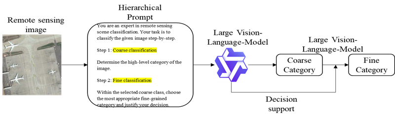
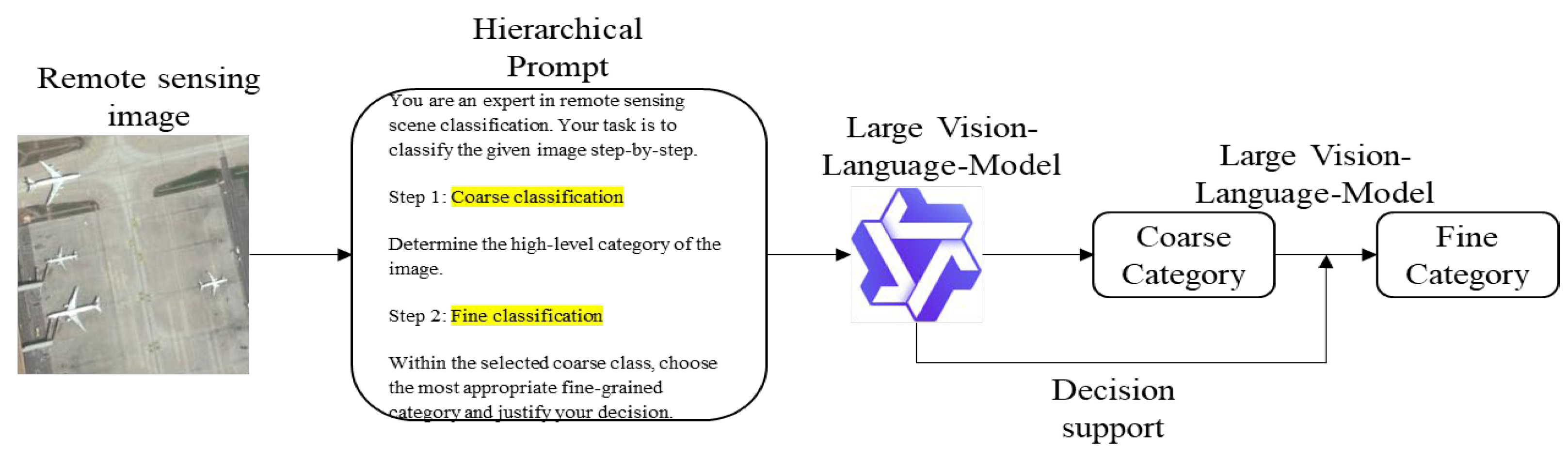
Figure 1.
Implementation of the hierarchical prompting pipeline.
Prompt engineering has emerged as a crucial technique for adapting pretrained VLMs to downstream tasks without requiring extensive retraining. Structured prompt designs have been shown to significantly influence model outputs by steering attention and reasoning pathways [11,12]. Hierarchical reasoning strategies [21,22], which decompose complex classification tasks into sequential sub-decisions, further align model processing with human cognitive mechanisms and have been successfully applied in few-shot and multimodal contexts [13,25,26].
Parameter-efficient fine-tuning approaches, such as Low-Rank Adaptation (LoRA) [14] and Quantized LoRA (QLoRA) [15], have been proposed to enable the efficient adaptation of large models with minimal computational overhead. These methods introduce a small number of trainable parameters into the frozen backbone of the model, allowing for rapid task-specific specialization without full-parameter updates. In resource-constrained environments or when fine-tuning ultra-large models, such techniques offer a practical alternative to traditional training pipelines, balancing performance gains with efficiency.
Building upon these prior advancements, this work explores the integration of hierarchical prompting and LoRA-based fine-tuning to adapt large vision-language models for remote sensing scene classification, aiming to bridge the gap between general-purpose multimodal pretraining and specialized geospatial applications.
3. Materials and Methods
We present our hierarchical prompting framework for coarse-to-fine remote sensing classification.
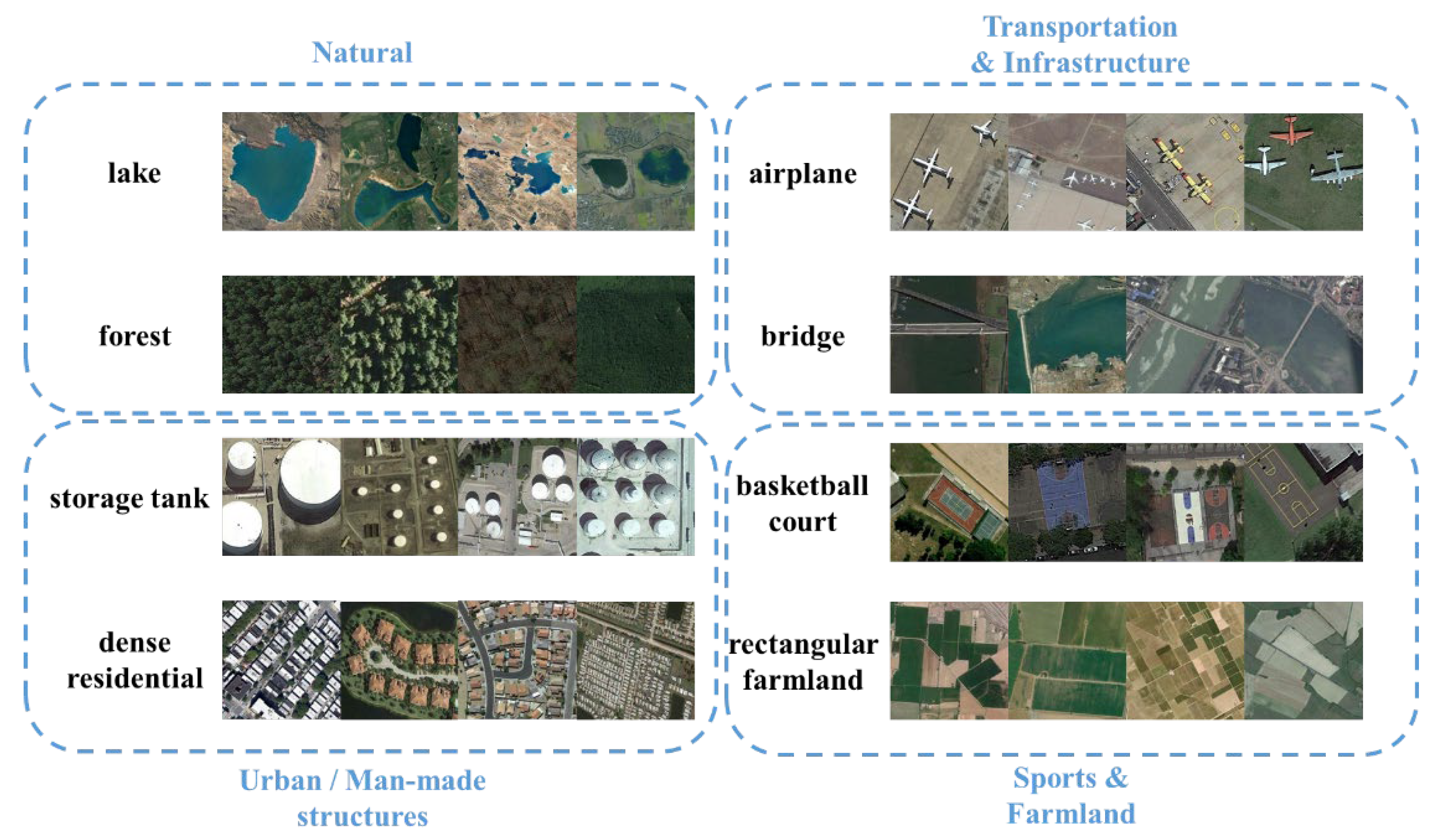
Figure 2.
Example Images of Selected Categories from the AID Dataset.
3.1. AID Dataset Preparation
We construct five versions of the Aerial Image Dataset (AID) to progressively improve data quality for evaluation. is the original dataset with 45 categories and no augmentation. applies standard geometric transformations to expand the data. performs augmentation only on the training set after a predefined split. refines the dataset by merging similar categories and cleaning ambiguous samples. applies post-cleaning augmentation based on . These steps systematically enhance generalization, address label noise, and create a more reliable benchmark [28]. Detailed dataset construction strategies are summarized in Table 1.
3.2. Prompt Design
To effectively guide large vision language models (VLMs) in remote sensing scene classification, we designed a series of progressively refined prompt templates, evolving from direct classification to hierarchical reasoning formats across versions to . The detailed prompt contents are provided in the Appendix A.
We design three prompt templates to guide model reasoning. requires direct category selection without explanation, emphasizing speed but risking misclassification. introduces a coarse-to-fine hierarchical process, where the model first selects a broad scene type and then a fine-grained class, providing explanations at each step to enhance interpretability. retains the hierarchical structure but streamlines the instructions, requiring concise outputs with brief justifications in a fixed format. Full prompt designs are detailed in Table 2.The adoption of a coarse-to-fine hierarchical structure is motivated by cognitive theories of visual recognition, where humans typically classify scenes by progressing from high-level to low-level categorizations. This approach reduces semantic confusion across unrelated categories, promotes focused discrimination within contextually similar options, and enhances classification accuracy, particularly in fine-grained tasks. Furthermore, requiring reasoning outputs fosters model self-validation and improves the transparency of the decision-making process, which is essential for trustworthy deployment in remote sensing applications.
Detailed construction rules of the dataset variants () and the rationale for aligning prompt styles with each variant are provided in Appendix B (Table A1).
3.3. External Evaluation Datasets and Label Mapping
We further evaluate cross-domain generalization on three small but widely used remote-sensing datasets: UC Merced [36] (UCM, 21 classes), WHU-RS19 [37] (19 classes), and RSSCN7 [38] (7 classes). To ensure a consistent hierarchy, classes from each dataset are mapped to our four coarse groups (Natural, Urban/Man-made, Transportation & Infrastructure, Sports & Farmland). Fine-grained evaluation is conducted on the intersection of class names with AID; non-overlapping classes contribute to the coarse metric only. Detailed class-name mapping is provided in Appendix C.
4. Experiments and Results
4.1. Experimental Setup
4.1.1. Hyperparameters
VLM Baselines. We used a fixed set of hyperparameters across all experiments unless otherwise specified. The learning rate was set to and the number of training epochs was typically 5, 10, or 15 depending on the experimental configuration. The primary training strategy was Low-Rank Adaptation (LoRA), while full fine-tuning and LoRA combined with DeepSpeed ZeRO-3 optimization [29] were also explored for comparison. A size scaling factor of 8 was employed by default, with some experiments adopting a larger factor of 28 to assess its impact on memory and performance. For large models such as Qwen2VL-72B and Qwen2.5VL-72B, 4-bit quantization was applied to enable efficient training and inference [30,31]. All experiments were implemented on the ms-swift framework [32] and optimized using the AdamW optimizer, with mixed-precision (FP16) training to accelerate convergence and improve computational efficiency.
CNN Baselines. To contextualize the benefits of hierarchical prompting beyond VLMs, we train classical CNNs under the same data splits and augmentations as our VLM experiments. We use ImageNet-pretrained ResNet-50, MobileNetV2 and EfficientNet-B0 with a linear classification head. Training uses SGD with momentum 0.9, cosine learning-rate decay from 0.01, weight decay 1e-4, label smoothing 0.1, batch size 64, early stopping (patience=5), and a maximum of 5 epochs. We report Top-1 accuracy and macro-F1, and profile efficiency (trainable parameters, peak GPU memory) to assess deployability.
4.1.2. Evaluation Metrics
To evaluate the performance of the models, we primarily adopted top-1 accuracy and macro f1 score as the metric for both coarse- classification and fine-classification tasks. Coarse-classification accuracy measures the model’s ability to correctly classify images into high-level categories such as Natural, Urban/Man-made, Transportation & Infrastructure, and Sports & Farmland. Fine-grained accuracy evaluates the correctness within each coarse category, targeting specific sub-classes. Additionally, we report per-category coarse accuracy to analyze model performance across different scene types. All results are reported on the validation set corresponding to each dataset split.
4.2. Main Results
4.2.1. Prompt Engineering Analysis
We compare three prompt versions (V0–V2) with Qwen2VL-72B and Qwen2.5VL-7B, both fine-tuned using LoRA and evaluated in the ms-swift framework. V0 is a generic, unstructured instruction; V1 introduces explicit coarse→fine hierarchical cues aligned with the label taxonomy; V2 preserves the same hierarchical content as V1 but expresses it in a more compact format. Across both model scales, the decisive factor is the presence of hierarchical guidance: moving from V0 to V1 increases Top-1 accuracy from 29.33% → 52.00% on Qwen2VL-72B and from 90.67% → 96.44% on Qwen2.5VL-7B, whereas changing formatting alone (V1→V2) yields only marginal differences (51.78% vs. 52.00% for 72B; 96.11% vs. 96.44% for 7B). These results indicate that structuring the decision process to mirror the label hierarchy—rather than cosmetic prompt reformatting—drives the gains, with noticeable error reductions in categories prone to cross-group confusion (e.g., Transportation & Infrastructure, Urban/Man-made). Overall, the quantitative trends are summarized in Table 3 and visualized in Figure 3, confirming that hierarchical prompting delivers model-agnostic improvements while formatting choice is secondary.
4.2.2. Model Architecture Comparison
To isolate the effect of architecture, we compare Qwen2VL-72B with its upgraded variant Qwen2.5VL-72B, both fine-tuned via LoRA under 4-bit quantization with an identical prompting/training protocol. The upgraded model delivers a substantial gain in coarse-level classification, raising Top-1 accuracy from 51.78% to 96.56% (+44.78 pp). Consistent improvements appear in every coarse category: Natural improves from 44.62% to 93.85%, Urban / Man-made from 13.64% to 78.64%, Transportation & Infrastructure from 18.08% to 91.15%, and Sports & Farmland from 2.50% to 95.00%. The coarse-level confusion matrices show markedly cleaner diagonals and far fewer cross-group confusions for Qwen2.5VL, particularly within classes that are small-scale or visually ambiguous, whereas Qwen2VL exhibits frequent misallocations across these groups. Taken together, these results (summarized in Table 4 and visualized in Figure 4 and Figure 5) indicate that the architectural advances in Qwen2.5VL—enhancing multimodal representation and vision–language alignment—are pivotal for robust remote-sensing scene understanding under the same fine-tuning and quantization budget.
4.2.3. Effect of Model Size
To assess parameter scaling under the same training budget, we compare Qwen2.5VL-7B and Qwen2.5VL-72B, both fine-tuned with LoRA and evaluated under identical settings and hierarchical prompts. Despite the >10× gap in parameter count, the coarse-level Top-1 accuracy improves only marginally from 96.11% (7B) to 96.56% (72B). Category-wise trends are similarly modest: Natural rises from 92.31% to 93.85%, Transportation & Infrastructure from 90.77% to 91.15%, and Sports & Farmland from 89.38% to 95.00%, whereas Urban / Man-made slightly decreases from 81.36% to 78.64%. The coarse confusion matrices show clean diagonals for both models, with the 72B variant exhibiting only a slightly sharper separation; overall differences do not scale proportionally with model size. Taken together, these results (summarized in Table 5 and visualized in Figure 6 and Figure 7) indicate that—once hierarchical prompting provides a strong inductive bias—smaller VLMs such as Qwen2.5VL-7B deliver competitive accuracy with a far better cost–efficiency profile, while scaling to 72B yields only incremental gains in this setting.
4.2.4. Data Version Impact
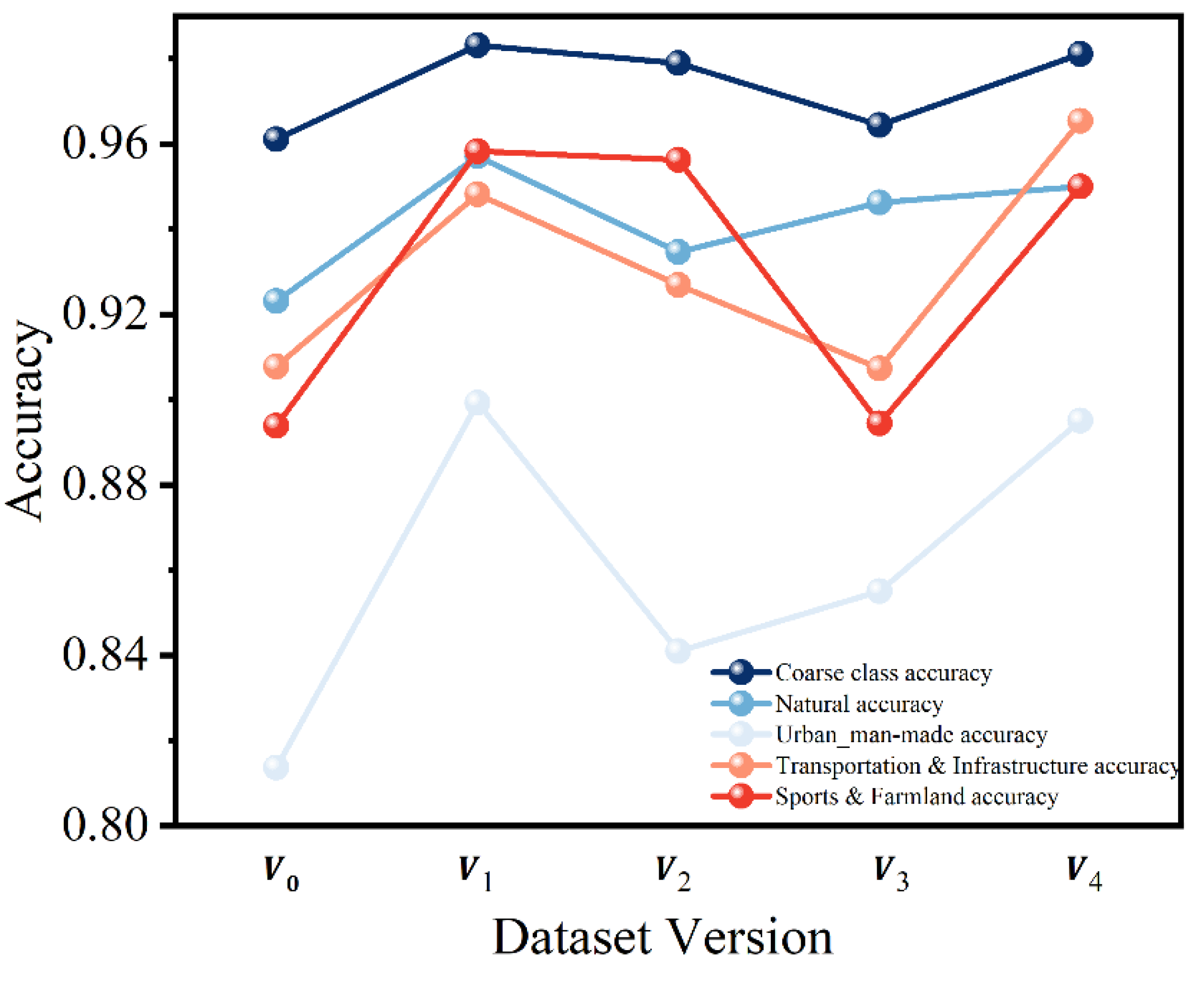
We assess the influence of dataset versions on classification performance across five variants (–), involving progressive data augmentation, class merging, and dataset cleaning strategies.Overall, versions and achieve the best results, highlighting the importance of dataset construction for model generalization.
Specifically, , with extensive augmentation techniques such as rotation and flipping, boosts the recognition of minority classes, achieving a coarse classification accuracy of 98.31% and notable gains in Natural (95.71%), Urban / Man-made (89.92%), Transportation & Infrastructure (94.81%), and Sports & Farmland (95.83%)., integrating both category refinement and data augmentation, maintains competitive performance with 98.11% coarse accuracy and particularly excels in the Transportation & Infrastructure class (96.53%).
In contrast, and exhibit slight degradations, especially in the Urban category, suggesting that aggressive restructuring without adequate data diversity may impair fine-classification discrimination.
These results demonstrate that data augmentation and semantic refinement are crucial for enhancing model robustness, while indiscriminate dataset restructuring may have adverse effects, particularly for complex scene classification.
Figure 8.
Accuracy Trends Across Dataset Versions.
4.2.5. Training Strategy Comparison
We compare LoRA-based tuning with full fine-tuning on Qwen2.5VL-7B under identical data, prompts, and optimization settings. At the coarse level, the two strategies are essentially indistinguishable—96.11% for LoRA versus 96.00% for full tuning. Class-wise differences are small and mixed (Table 6): Natural and Urban / Man-made are marginally higher with full tuning (93.08% vs. 92.31%, 81.82% vs. 81.36%), whereas Transportation & Infrastructure and Sports & Farmland favor LoRA (90.77% vs. 90.38%, 89.38% vs. 88.12%). The coarse confusion matrices (Figure 9) show similarly clean diagonals for both strategies, and the bar plots (Figure 10) confirm that variations remain within about one percentage point across categories. Taken together, these results indicate that LoRA matches the accuracy of full tuning while adapting only a small fraction of parameters, leading to substantially lower memory and training cost. For remote-sensing deployments where compute and energy are constrained, LoRA offers a more practical path without sacrificing classification performance.
4.2.6. Comparison with Classical CNNs
Setup. Table 7 compares three ImageNet-pretrained CNNs (ResNet-50 [33], MobileNetV2 [34], EfficientNet-B0 [35]) with our VLM (Qwen2.5-VL-7B) fine-tuned via LoRA under the proposed hierarchical prompting. All methods use the same AID- split and the same augmentations to ensure fairness. We report fine class Top-1 accuracy, macro-F1, the number of trainable parameters, and peak GPU memory.
Results and analysis. The hierarchical-prompted VLM achieves the best accuracy: 91.33% Top-1 and 91.32% macro-F1, surpassing ResNet-50 by +0.66 / +0.86 points, MobileNetV2 by +1.55 / +1.51 points, and EfficientNet-B0 by +0.22 / +0.23 points, respectively. The improvement is slightly larger on macro-F1 than on Top-1, indicating better class-balance and sensitivity to minority categories. In terms of tunable parameters, LoRA updates 8.39M parameters—only ~35.6% of ResNet-50’s 23.60M trainable parameters (and far below full 7B fine-tuning)—while CNNs require updating all model weights end-to-end. As expected, the VLM incurs higher peak memory (14.00 GB) than CNNs (2.63–3.14 GB), but remains feasible on a single modern GPU and substantially reduces the number of parameters that must be optimized.
Takeaway. Under matched data and augmentations, hierarchical prompting on a VLM delivers consistent accuracy gains over strong CNN baselines while requiring fewer trainable parameters than end-to-end CNN training. The trade-off is higher VRAM usage, which is acceptable for workstation-class GPUs. These results demonstrate tangible benefits beyond classical CNNs, supporting the practicality of the proposed approach when memory resources are available.
4.2.7. Data Efficiency Under Limited Labels
Setup. To evaluate label efficiency, we randomly subsample 1% / 5% / 10% / 25% of the training labels on AID- while keeping the validation sets unchanged. We compare three ImageNet-pretrained CNNs (ResNet-50, MobileNetV2, EfficientNet-B0) with our Qwen2.5-VL-7B + LoRA under hierarchical prompting. All other settings (split, augmentations, optimizer) follow Sec. 4.1; LoRA uses early stopping. Results (Top-1 / Macro-F1, %) are averaged over the same seeds and reported in Table 8.
Results and analysis. At 1% labels, the hierarchical-prompted VLM reaches 81.44 / 82.63, outperforming the best CNN (MobileNetV2, 53.44 / 53.46) by +28.00 / +29.17 points, and exceeding ResNet-50 by +53.55 / +56.38. At 5% labels, our method attains 87.22 / 87.90, ahead of MobileNetV2 (67.00 / 65.94) by +20.22 / +21.96; notably, it already surpasses EfficientNet-B0 at 25% (86.22 / 86.13) and ResNet-50 at 25% (84.33 / 84.22). At 10% labels, the VLM obtains 85.22 / 84.92, still better than ResNet-50 (69.44 / 69.44) and EfficientNet-B0 (75.00 / 74.51), and slightly above MobileNetV2 at the same fraction (81.11 / 80.98; +4.11 / +3.94). At 25% labels, MobileNetV2 (90.00 / 89.94) becomes competitive and slightly surpasses the VLM (87.11 / 87.04, −2.89 / −2.90), reflecting the well-known scaling of CNNs with abundant labels. Across all fractions, however, the VLM maintains high and stable performance with far fewer annotated samples.
Label-efficiency takeaway. The hierarchical-prompted VLM exhibits strong data efficiency: with only 1% labels it matches/exceeds MobileNetV2 trained on 10% labels (≈10× fewer labels), and with 5% labels it already outperforms ResNet-50/EfficientNet-B0 trained on 25% labels (≈5× fewer labels). These results indicate that hierarchical prompting leverages VLM priors to deliver high accuracy under scarce supervision, while CNNs need substantially more labels to reach comparable performance.
4.2.8. Cross-Domain Generalization
To assess whether the model trained on AID generalizes beyond its source domain, we evaluate on three small but widely used remote-sensing datasets—UC Merced (UCM), WHU-RS19, and RSSCN7—without changing the prompting pipeline. Because the fine-classification taxonomies of these datasets differ from AID (e.g., heterogeneous splits of residential/urban sub-classes), we report coarse-level metrics only (Top-1 accuracy and Macro-F1) for fair, cross-dataset comparison. The class-name mapping to our four coarse groups is provided in the Supplementary Material. Training details (optimizer, early stopping, label smoothing) follow Section 4.1.
We consider two protocols: Zero-shot, where the model trained on AID-V2 is evaluated directly on the target dataset; and Few-shot LoRA, where we adapt the model with K=16 labeled samples per class on the target dataset for ≤5 epochs using LoRA (lightweight parameter-efficient tuning). Table 9 summarizes the results. Zero-shot generalization is already strong on UCM (87.20% Top-1 / 87.04% F1) and WHU-RS19 (93.90% / 91.98%), while RSSCN7 is more challenging due to class imbalance and texture shifts (74.07% / 28.11%). With few-shot LoRA, performance improves consistently across all targets: UCM gains +8.50 Top-1 and +8.51 F1 (to 95.70% / 95.55%), WHU-RS19 gains +2.91 / +3.94 (to 96.81% / 95.92%), and RSSCN7 gains +8.30 / +34.53 (to 82.37% / 62.64%). These results indicate that (i) the hierarchical prompting framework transfers well in a zero-shot manner, and (ii) minimal labeled data and lightweight LoRA adaptation suffice to bridge remaining domain gaps efficiently.
Note that zero-shot numbers for AID-V2 are not applicable (marked “—“) because AID-V2 serves as the source training set. Full implementation details and the class-mapping tables are released with the code.
4.3. Hierarchical Multi-Label Extension
Remote-sensing scenes frequently contain multiple coexisting semantics (e.g., forest + river, residential + road). Our framework naturally extends to hierarchical multi-label classification by predicting a probability for each node in the label tree and enforcing parent–child consistency.
Label tree and outputs. Let denote the label hierarchy (coarse → fine). For every node the model outputs a logit and probability . Ground-truth labels are multi-hot vectors that can activate multiple leaves and their ancestors.
Loss. We optimize a hierarchical binary cross-entropy with a consistency regularizer:
which discourages a child being more probable than its parent and promotes coherent top-down predictions. This loss is model-agnostic and plugs into our LoRA/QLoRA heads without changing the VLM backbone.
Inference (top-down decoding).
- Start from the root; apply a calibrated threshold for each node.
- If , expand to its children; otherwise prune the subtree.
- Return all activated leaves and (optionally) their ancestors. A simple repair step sets to satisfy ancestry.
Prompting. The hierarchical prompts remain unchanged; we only instruct the model to “list all applicable fine-classes” within the selected coarse branch and to justify each label briefly. This keeps the coarse→fine reasoning intact while allowing multiple fine labels.
Evaluation. We recommend reporting mAP, micro/macro-F1, and a hierarchical-F1 (counting a leaf as correct only if its ancestors are also correct). This complements the top-1 accuracy used in the single-label setting.
Practical note. When the training set is single-label (e.g., AID), the above can be used as-is by treating the single label as an active leaf and implicitly activating its ancestors; true multi-label behavior can be fully validated on public multi-label RS datasets and is left as future work.
5. Conclusions
This work investigated hierarchical (coarse→fine) prompting for remote-sensing scene understanding with parameter-efficient adaptation (LoRA/QLoRA) under leakage-safe data protocols. Across extensive ablations and cross-domain evaluations (Secs. 4.2.6–4.2.8), we show that the proposed pipeline improves accuracy, interpretability, and data efficiency while keeping training and memory costs practical.
5.1. Effectiveness of Hierarchical Prompting
Hierarchical prompting consistently strengthens classification by decomposing decisions into coarse then fine stages, which reduces the search space, curbs semantic confusion, and aligns with expert practice (broad context before detail). The fine stage also acts as an explicit self-check constrained by the selected coarse category, yielding more deliberate and interpretable outputs. Beyond in-domain gains, zero-shot tests on UCM/WHU-RS19/RSSCN7 (Sec. 4.2.6) show that hierarchical prompting retains its advantages under domain shift when evaluated with a consistent label hierarchy (coarse metrics for all classes; fine metrics on class intersections with AID). Moreover, few-shot LoRA adaptation (Sec. 4.2.7/4.2.8) further boosts target-domain performance with only a handful of labeled samples per class and ≤5 training epochs, indicating strong data efficiency and practical deployability.
5.2. Trade-offs Between Model Size and Accuracy
Larger models (e.g., Qwen2.5VL-72B) offer higher peak accuracy on visually subtle cases, but improvements diminish with scale, and the extra cost in memory, wall-time, and deployment complexity grows steeply. Mid-sized/backbone-efficient settings combined with LoRA/QLoRA strike a favorable balance, delivering accuracy close to full fine-tuning with a small fraction of trainable parameters. In addition, comparisons against classical CNN baselines confirm that the gains stem from the coarse→fine reasoning itself rather than sheer model size: the hierarchy adds robustness to acquisition changes and class imbalance while keeping compute modest. Finally, few-shot LoRA on target datasets provides a lightweight path to close most of the remaining domain gap without retraining the full model.
5.3. Limitations and Potential Failure Cases
Several limitations remain. Coarse-stage errors propagate to the fine stage, so early mistakes can bias final decisions; confidence-aware repair or joint decoding is a promising remedy. Fine-classification errors persist for visually overlapping classes (e.g., texture-centric categories) and for datasets whose taxonomies do not perfectly align with AID—some external classes are generic (e.g., Buildings, Agriculture), hence evaluated at the coarse level only. Results can be sensitive to prompt phrasing in mid-sized models; prompt calibration or instruction distillation may reduce variance. While 4-bit quantization and LoRA lower resource demands, real-time onboard inference under strict SWaP constraints and very-large-model scaling still require further engineering.
5.4. Future Work
Our framework naturally extends to hierarchical multi-label prediction using node-wise probabilities, consistency-aware losses, and top-down decoding; we will conduct a dedicated evaluation on multi-label remote-sensing corpora, including threshold calibration and imbalance-aware training. Future directions also include: (i) prompt-robust or prompt-free variants via distillation; (ii) broader cross-sensor generalization (e.g., SAR/multispectral) and temporal reasoning; (iii) tighter domain-gap diagnostics with feature-space metrics; and (iv) compression/acceleration tailored to onboard UAV deployment.
Appendix A. Prompt Templates
To ensure reproducibility and transparency of our prompt design, we provide the complete templates used in different dataset versions below.
A.1. Prompt: Direct Category Selection
<image>
You must choose **only one** category name from the following list that best matches the image. Do not explain. Just return the category name exactly as it appears.
Categories: {category_str}
A.2. Prompt: Coarse-to-Fine Step-by-Step Classification
<image>
You are an expert in remote sensing scene classification. Your task is to classify the given image step-by-step. Follow this two-step reasoning process:
### Step 1: Coarse classification
Determine the high-level category of the image based on the following four options:
1. Natural:
- mountain, lake, forest, beach, cloud, desert, island, river, meadow, snowberg, sea_ice, chaparral, wetland
2. Urban / Man-made:
- dense_residential, medium_residential, sparse_residential, mobile_home_park, industrial_area, commercial_area, church, palace, storage_tank, terrace, thermal_power_station
3. Transportation & Infrastructure:
- airport, airplane, freeway, bridge, railway, railway_station, harbor, intersection, overpass, roundabout, runway, parking_lot, ship
4. Sports & Farmland:
- baseball_diamond, basketball_court, tennis_court, golf_course, ground_track_field, stadium, circular_farmland, rectangular_farmland
Explain your reasoning and select one coarse class.
### Step 2: Fine classification
Within the selected coarse class, choose the most appropriate fine-grained category and justify your decision.
Expected output format:
|<Coarse class>|XXX|<Fine class>|XXX|<Reasoning>|XXX
A.3. Prompt: Streamlined Coarse-to-Fine Reasoning
<image>
You are an expert in remote sensing scene classification. Your task is to classify the given image step-by-step.
Step 1: Coarse classification
Determine the high-level category of the image.
Step 2: Fine classification
Within the selected coarse class, choose the most appropriate fine-grained category and justify your decision.
Expected output format:
|<Coarse class>|XXX|<Fine class>|XXX|<Reasoning>|XXX
Appendix B. Dataset Variant Design and Prompt–Variant Alignment
B.1. Goals
We define five protocol variants to stress different robustness axes and to keep prompt design purposeful rather than ad-hoc: baseline comparability, orientation/flip invariance, leakage-safe augmentation, semantic cleaning, and the combined setting.
B.2. Variant Construction and Prompt Rationale (Table A1).

Table A1.
Construction rules and why each variant uses a specific prompt style.
| Variant | Design goal (robustness axis) | Construction rule (leakage control) | Prompt alignment (why this prompt) | Artifacts |
| Baseline comparability | Standard random split; no augmentation | Generic flat prompt, used as the neutral reference | Split index (train/val/test) | |
| Orientation/flip invariance stress | Global rotations (0/90/180/270) and H/V flips applied naïvely | Add orientation-invariant wording and spatial cues | Augmentation list | |
| Leakage-safe augmentation | Split-before-augment: apply all augmentations only to training; validation/test untouched | Keep wording to isolate protocol effect (naïve vs. leakage-safe) | Train-only aug manifests | |
| Semantic disambiguation / label noise | Merge near-synonymous/ambiguous classes; remove borderline samples; run near-duplicate audit across splits | Emphasize structural/semantic descriptors in a coarse→fine template | Cleaned indices + audit logs | |
| Clean + invariance (combined) | Apply’s leakage-safe augmentation aftercleaning | Streamlined hierarchical prompt (coarse→fine) for efficiency and clarity | All manifests & scripts |
B.3. Leakage Prevention and Duplicate Audit
Adopt split-before-augment: generate the split first, then apply augmentations only to the training subset.
Screen near-duplicates across splits via perceptual image hashing; compute pairwise Hamming distances and remove pairs below a fixed threshold τ (chosen from the distance histogram; the exact τ and logs are released with the scripts).
Manually spot-check borderline cases to avoid class drift.
Release indices, augmentation manifests and audit logs for exact reproducibility.
B.4. Reproducibility
We release (i) the split files for –, (ii) augmentation recipes, and (iii) the prompt templates used in each variant, together with training seeds and code for re-running all results. https://github.com/qlj215/HPE-RS
Appendix C. Label Mapping for External Datasets
C.1. Mapping Policy and Notation
To ensure a consistent evaluation hierarchy across datasets, each external class is mapped to one of our four coarse groups—Natural, Urban / Man-made, Transportation & Infrastructure, Sports & Farmland—and, when there is an exact or 1-to-1 synonym match, to an AID fine class. If no exact fine-level counterpart exists, the class contributes coarse metrics only (“—“ in the AID Fine Class column). Class names are matched case-insensitively with minor normalization (hyphen/underscore/space). Two authors independently verified all mappings; disagreements were resolved by discussion.
C.2. UC Merced (UCM) → Our Hierarchy / AID Fine Classes
Notes (no one-to-one AID fine match):
- 1)
- Agriculture — generic farmland (AID distinguishes circular vs. rectangular farmland).
- 2)
- Buildings — generic built-up category (AID uses more specific urban subclasses).
Table A2.
UC Merced (UCM, 21 classes) → Coarse groups.
| UCM Class | Coarse Class | UCM Class | Coarse Class | UCM Class | Coarse Class |
| Agriculture | Sports & Farmland | Forest | Natural | Overpass | Transportation & Infrastructure |
| Airplane | Transportation & Infrastructure | Freeway | Transportation & Infrastructure | Parking lot | Transportation & Infrastructure |
| Baseball diamond |
Sports & Farmland | Golf course | Sports & Farmland | River | Natural |
| Beach | Natural | Harbor | Transportation & Infrastructure | Runway | Transportation & Infrastructure |
| Buildings | Urban / Man-made | Intersection | Transportation & Infrastructure | Sparse residential |
Urban / Man-made |
| Chaparral | Natural | Medium residential | Urban / Man-made | Storage tanks | Urban / Man-made |
| Dense residential |
Urban / Man-made | Mobile home park | Urban / Man-made | Tennis court | Sports & Farmland |
C.3. WHU-RS19 → Our Hierarchy / AID Fine Classes
Notes (no one-to-one AID fine match):
- 1)
- Farmland — generic farmland (AID splits by geometry).
- 2)
- Park — urban green/parkland (no exact AID fine class).
- 3)
- Residential area — density not specified (AID separates dense/medium/sparse).
- 4)
- (Ambiguity handled at fine level but irrelevant here) Football field — could appear with or without athletics track; we evaluate at the coarse level.
Table A3.
WHU-RS19 (19 classes) → Coarse groups.
| WHU Class | Coarse Class | WHU Class | Coarse Class | WHU Class | Coarse Class |
| Airport | Transportation & Infrastructure | Football field | Sports & Farmland | Parking lot | Transportation & Infrastructure |
| Beach | Natural | Forest | Natural | Pond | Natural |
| Bridge | Transportation & Infrastructure | Industrial area | Urban / Man-made | Port | Transportation & Infrastructure |
| Commercial area | Urban / Man-made | Meadow | Natural | Railway station | Transportation & Infrastructure |
| Desert | Natural | Mountain | Natural | Residential area | Urban / Man-made |
| Farmland | Sports & Farmland | Park | Urban / Man-made | River | Natural |
| - | - | Viaduct | Transportation & Infrastructure | - | - |
C.4. RSSCN7 → Our Hierarchy / AID Fine Classes
Notes (no one-to-one AID fine match):
- 1)
- Field — generic farmland (AID splits circular/rectangular).
- 2)
- Residential — density not specified (AID distinguishes dense/medium/sparse).
Table A4.
RSSCN7 (7 classes) → Coarse groups.
| RSSCN7 Class | Coarse Class | RSSCN7 Class | Coarse Class | RSSCN7 Class | Coarse Class |
| Grass | Natural | Industrial | Urban / Man-made | Residential | Urban / Man-made |
| River | Natural | Field | Sports & Farmland | Parking | Transportation & Infrastructure |
| - | - | Forest | Natural | - | - |
References
- G. Cheng, J. Han, and X. Lu, “Remote sensing image scene classification: Benchmark and state of the art,” Proceedings of the IEEE, vol. 105, no. 10, pp. 1865–1883, Oct. 2017.
- G.-S. Xia, J. Hu, F. Hu, B. Shi, X. Bai, Y. Zhong, L. Zhang, and X. Lu, “AID: A Benchmark Dataset for Performance Evaluation of Aerial Scene Classification,” IEEE Transactions on Geoscience and Remote Sensing, vol. 55, no. 7, pp. 3965–3981, Jul. 2017.
- A. Radford, J. W. Kim, C. Hallacy, A. Ramesh, G. Goh, S. Agarwal, and I. Sutskever, “Learning Transferable Visual Models from Natural Language Supervision,” in Proceedings of the 38th International Conference on Machine Learning (ICML), Jul. 2021.
- J.-B. Alayrac, J. Donahue, P. Luc, A. Miech, I. Barr, Y. Li, et al., “Flamingo: A Visual Language Model for Few-Shot Learning,” arXiv preprint, arXiv:2204.14198, 2022.
- Yang, Yi and S. Newsam. “Bag-of-visual-words and spatial extensions for land-use classification.” ACM SIGSPATIAL International Workshop on Advances in Geographic Information Systems (2010).
- M. Castelluccio, G. Poggi, C. Sansone, and L. Verdoliva, “Land Use Classification in Remote Sensing Images by Convolutional Neural Networks,” arXiv preprint, arXiv:1508.00092, 2015.
- S. Basu, S. Ganguly, S. Mukhopadhyay, et al., “DeepSat: A Learning Framework for Satellite Imagery,” in Proceedings of the 23rd ACM SIGSPATIAL International Conference on Advances in Geographic Information Systems (SIGSPATIAL), 2015.
- G.-S. Xia, J. Hu, F. Hu, et al., “AID: A Benchmark Dataset for Performance Evaluation of Aerial Scene Classification,” IEEE Transactions on Geoscience and Remote Sensing, vol. 55, no. 7, pp. 3965–3981, Jul. 2017.
- Chen, Ting et al. “A Simple Framework for Contrastive Learning of Visual Representations.” ArXiv abs/2002.05709 (2020): n. pag.
- J.-B. Alayrac, J. Donahue, P. Luc, et al., “Flamingo: A Visual Language Model for Few-Shot Learning,” arXiv preprint, arXiv:2204.14198, 2022.
- T. Zhao, X. Wu, et al., “Exploring Prompt-Based Learning for Text-to-Image Generation,” arXiv preprint, arXiv:2203.08519, 2022.
- J. Gao, X. Han, et al., “Scaling Instruction-Finetuned Language Models,” arXiv preprint, 2022.
- X. Li, C. Yin, et al., “Decomposed Prompt Learning for Language Models,” in Advances in Neural Information Processing Systems (NeurIPS), 2022.
- E. Hu, Y. Shen, P. Wallis, et al., “LoRA: Low-Rank Adaptation of Large Language Models,” arXiv preprint, arXiv:2106.09685, 2021.
- Dettmers, Tim, et al. “Qlora: Efficient finetuning of quantized llms.” Advances in neural information processing systems 36 (2023): 10088-10115.
- Y. Zhang, Y. Wang, et al., “RemoteCLIP: A Vision–Language Foundation Model for Remote Sensing,” arXiv preprint, arXiv:2408.05554, 2024.
- Z. Luo, Y. Chen, et al., “RS5M: A Large-Scale Vision–Language Dataset for Remote Sensing,” in Proceedings of the IEEE/CVF Conference on Computer Vision and Pattern Recognition (CVPR), 2024.
- CSIG-RS Lab, “RSGPT: Visual Remote Sensing Chatbot,” ISPRS Journal of Photogrammetry and Remote Sensing, 2024.
- Y. Li, J. Zhang, et al., “GeoChat: Grounded Vision–Language Model for Remote Sensing,” IEEE Transactions on Geoscience and Remote Sensing, early access, 2024.
- Z. Luo, X. Xie, et al., “VRSBench: A Versatile Vision–Language Benchmark for Remote Sensing,” in Advances in Neural Information Processing Systems (NeurIPS), 2023.
- Y. Bazi, M. Al Rahhal, et al., “RS-LLaVA: A Large Vision–Language Model for Joint Captioning and VQA in Remote Sensing,” Remote Sensing, vol. 16, no. 9, p. 1477, 2024.
- Z. Zhang, X. Li, et al., “EarthGPT: A Universal MLLM for Multi-Sensor Remote Sensing,” arXiv preprint, arXiv:2401.16822, 2024.
- G.-S. Xia, J. Hu, F. Hu, et al., “NWPU-RESISC45: A Public Dataset for Remote Sensing Image Scene Classification,” in Proceedings of the IEEE Conference on Computer Vision and Pattern Recognition (CVPR) Workshops, 2017.
- P. Helber, B. Bischke, A. Dengel, and D. Borth, “EuroSAT: A Novel Dataset and Deep Learning Benchmark for Land Use and Land Cover Classification,” IEEE Journal of Selected Topics in Applied Earth Observations and Remote Sensing, 2019.
- J. Wei, X. Wang, D. Schuurmans, et al., “Chain-of-Thought Prompting Elicits Reasoning in Large Language Models,” arXiv preprint, 2022.
- S. Yao, Y. Yu, J. Zhao, et al., “Tree-of-Thoughts: Deliberate Problem Solving with Large Language Models,” arXiv preprint, 2023.
- B. Barz and J. Denzler, “Do We Train on Test Data? Purging CIFAR of Near-Duplicates,” arXiv preprint, arXiv:1902.00423, 2019.
- C. Zauner, “Implementation and Benchmarking of Perceptual Image Hash Functions,” Master’s thesis, 2010.
- S. Rajbhandari, J. R. Child, D. Li, et al., “ZeRO: Memory Optimizations Toward Training Trillion-Parameter Models,” in Proceedings of the International Conference for High Performance Computing, Networking, Storage and Analysis (SC ’20), 2020.
- T. Dettmers, M. Lewis, S. Shleifer, and L. Zettlemoyer, “LLM.int8(): 8-Bit Matrix Multiplication for Transformers at Scale,” arXiv preprint, 2022.
- Xu, Y., Xie, L., Gu, X., Chen, X., Chang, H., Zhang, H., Chen, Z., Zhang, X., & Tian, Q. (2024). QA-LoRA: Quantization-Aware Low-Rank Adaptation of Large Language Models. ICLR 2024.
- W. Zhao, H. Xu, et al., “SWIFT: A Scalable Lightweight Infrastructure for Fine-Tuning,” in Proceedings of the AAAI Conference on Artificial Intelligence (AAAI), 2025.
- K. He et al., “Deep Residual Learning for Image Recognition,” CVPR, 2016.
- M. Sandler et al., “MobileNetV2: Inverted Residuals and Linear Bottlenecks,” CVPR, 2018.
- M. Tan and Q. Le, “EfficientNet: Rethinking Model Scaling for CNNs,” ICML, 2019.
- Neumann M, Pinto A S, Zhai X, et al. In-domain representation learning for remote sensing[J]. arXiv preprint arXiv:1911.06721, 2019.
- D. Dai and W. Yang, “Satellite image classification via two-layer sparse coding with biased image representation,” IEEE Geoscience and Remote Sensing Letters, vol. 8, no. 1, pp. 173–176, 2011.
- Q. Zou, L. Ni, T. Zhang, and Q. Wang, “Deep learning based feature selection for remote sensing scene classification,” IEEE Geoscience and Remote Sensing Letters, vol. 12, no. 11, pp. 2321–2325, Nov. 2015, . [CrossRef]
Figure 3.
Top-1 accuracy comparison between different prompt version.
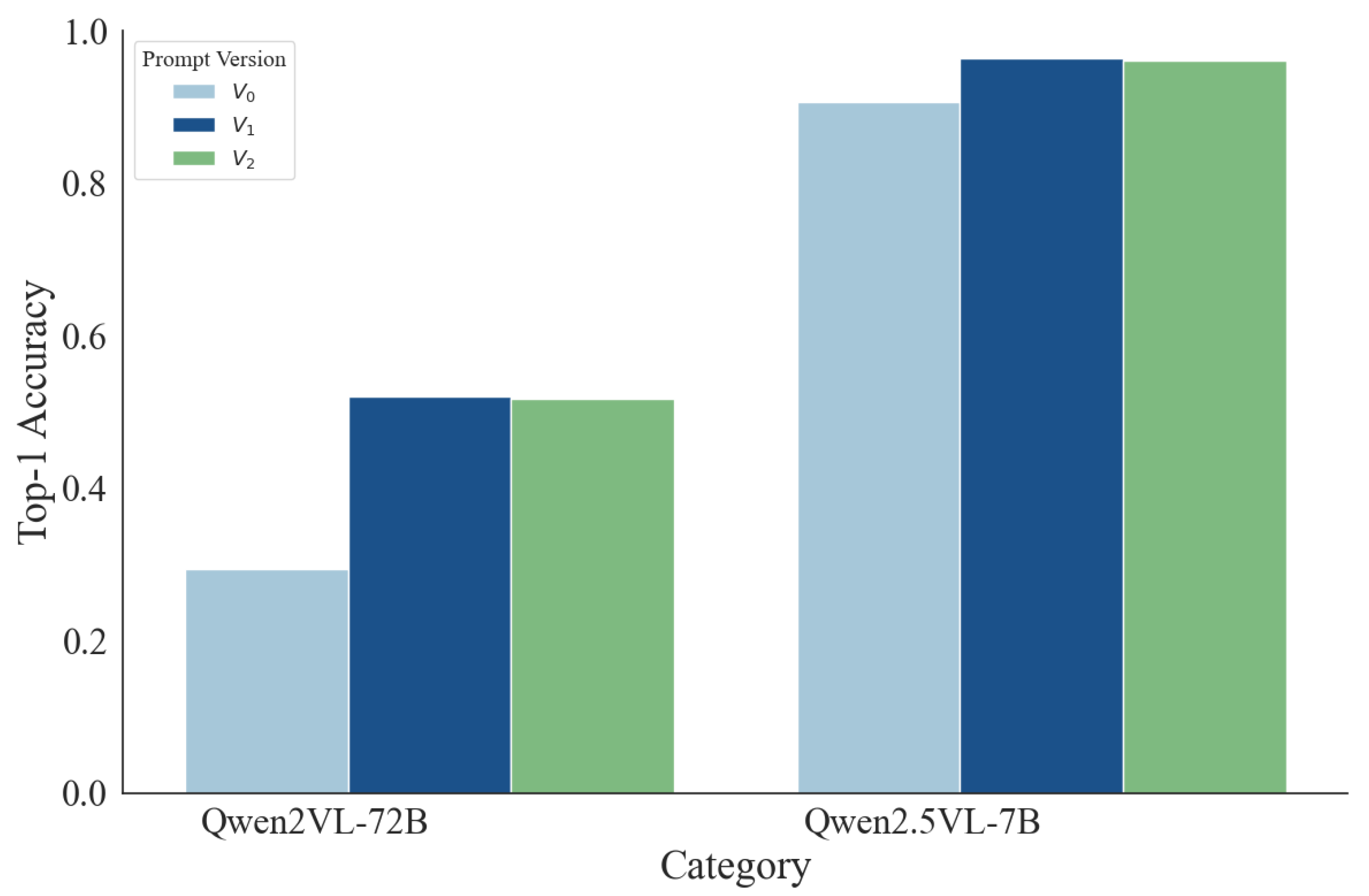
Figure 4.
Coarse-level confusion matrix of Qwen2-based and Qwen2.5-based model. (l) Coarse-level confusion matrix of Qwen2-based model. (r) Coarse-level confusion matrix of Qwen2.5-based model.
Figure 4.
Coarse-level confusion matrix of Qwen2-based and Qwen2.5-based model. (l) Coarse-level confusion matrix of Qwen2-based model. (r) Coarse-level confusion matrix of Qwen2.5-based model.
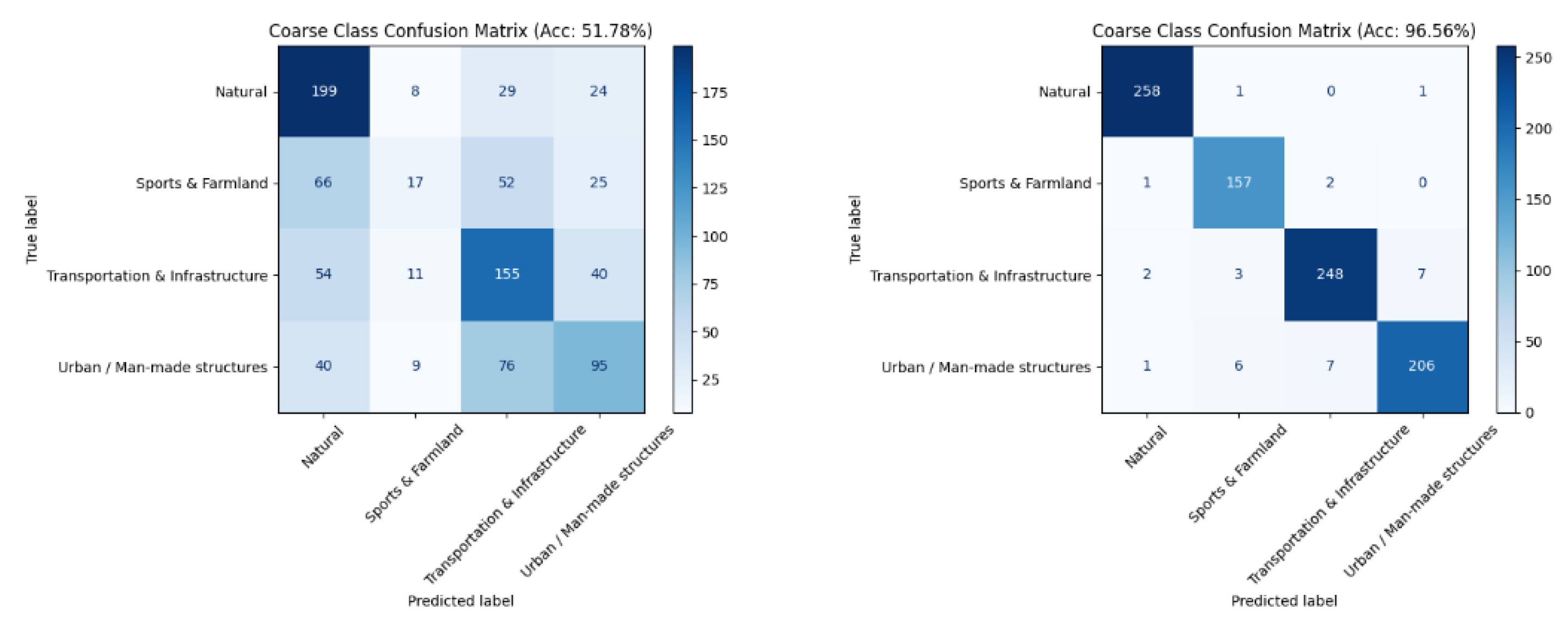
Figure 5.
Top-1 accuracy comparison between models based on Qwen2.5 and Qwen2 architectures.
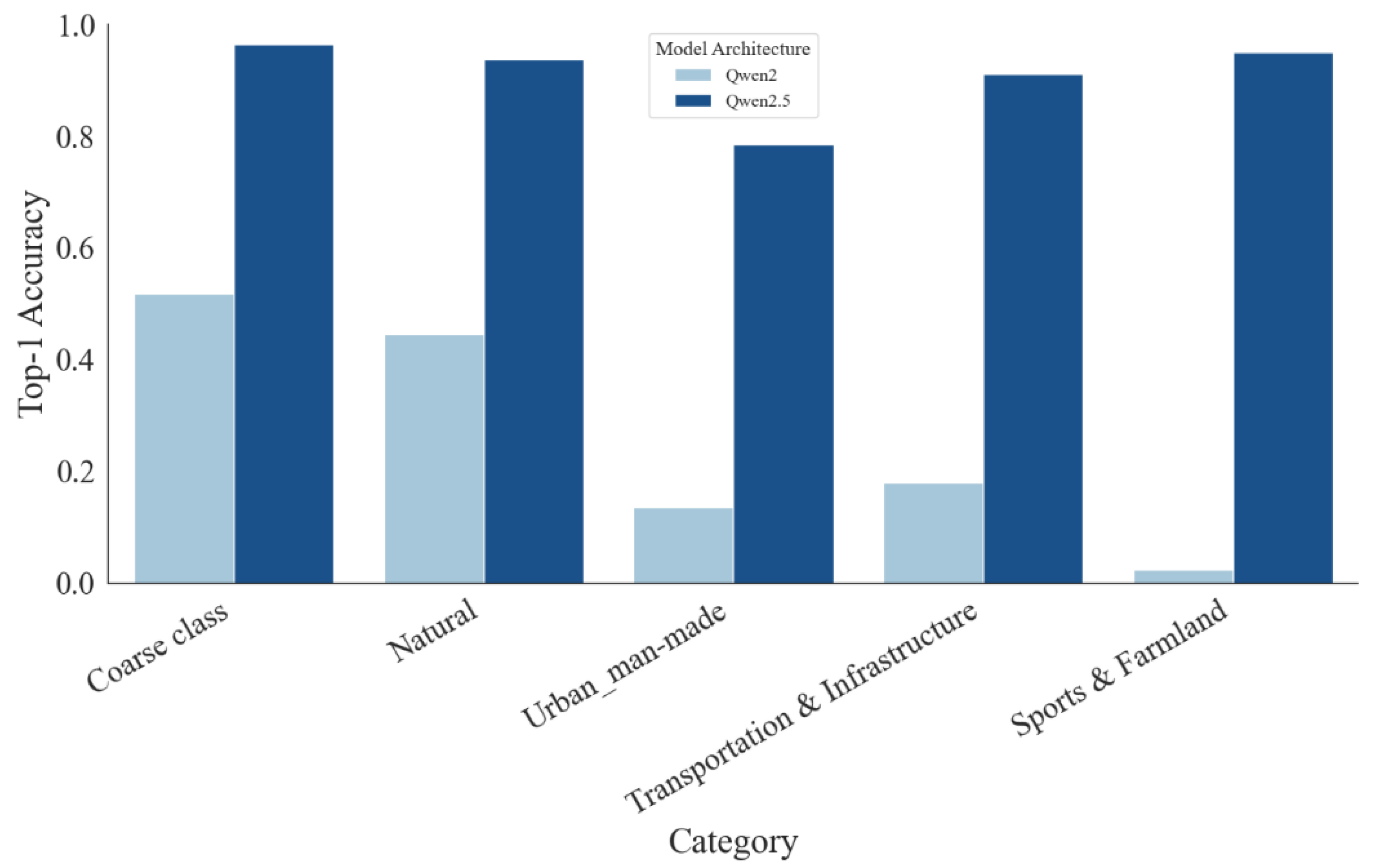
Figure 6.
Coarse-level confusion matrix of 7B and 72B models based on Qwen2.5 architecture. (l) Coarse-level confusion matrix of 7B model. (r) Coarse-level confusion matrix of 72B model.
Figure 6.
Coarse-level confusion matrix of 7B and 72B models based on Qwen2.5 architecture. (l) Coarse-level confusion matrix of 7B model. (r) Coarse-level confusion matrix of 72B model.
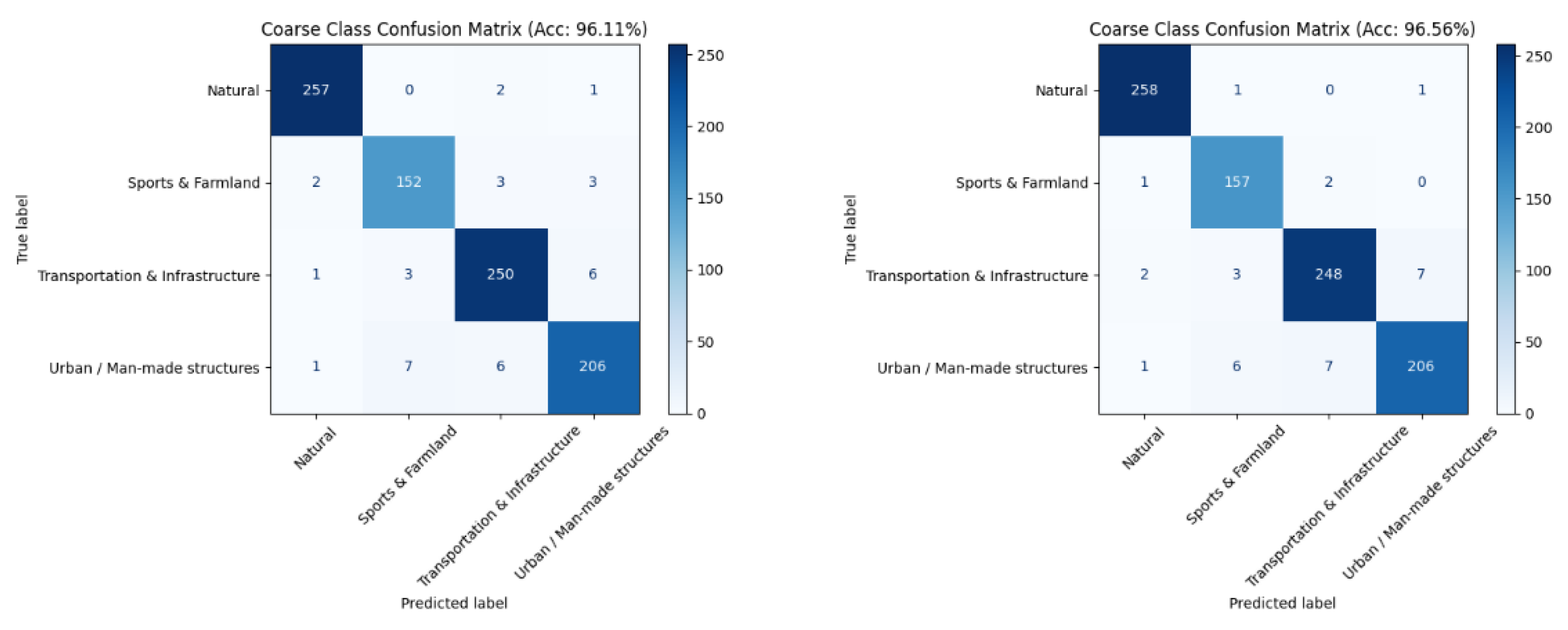
Figure 7.
Top-1 accuracy comparison between 7B and 72B models based on Qwen2.5 architecture.
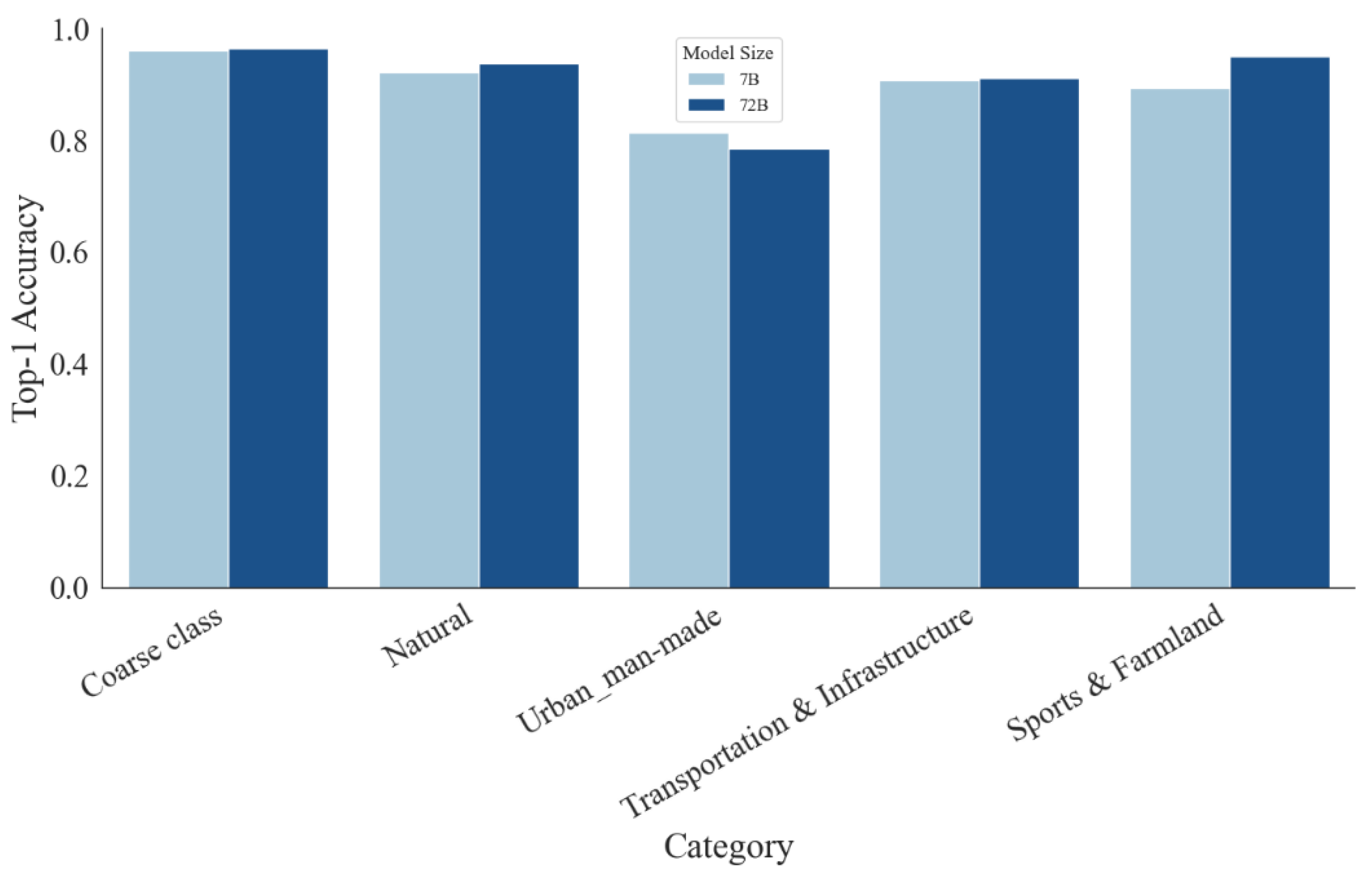
Figure 9.
Coarse-level confusion matrix of different training strategy. (l) Coarse-level confusion matrix of LoRA-based tuning strategy. (r) Coarse-level confusion matrix of 72B full-tuning strategy.
Figure 9.
Coarse-level confusion matrix of different training strategy. (l) Coarse-level confusion matrix of LoRA-based tuning strategy. (r) Coarse-level confusion matrix of 72B full-tuning strategy.
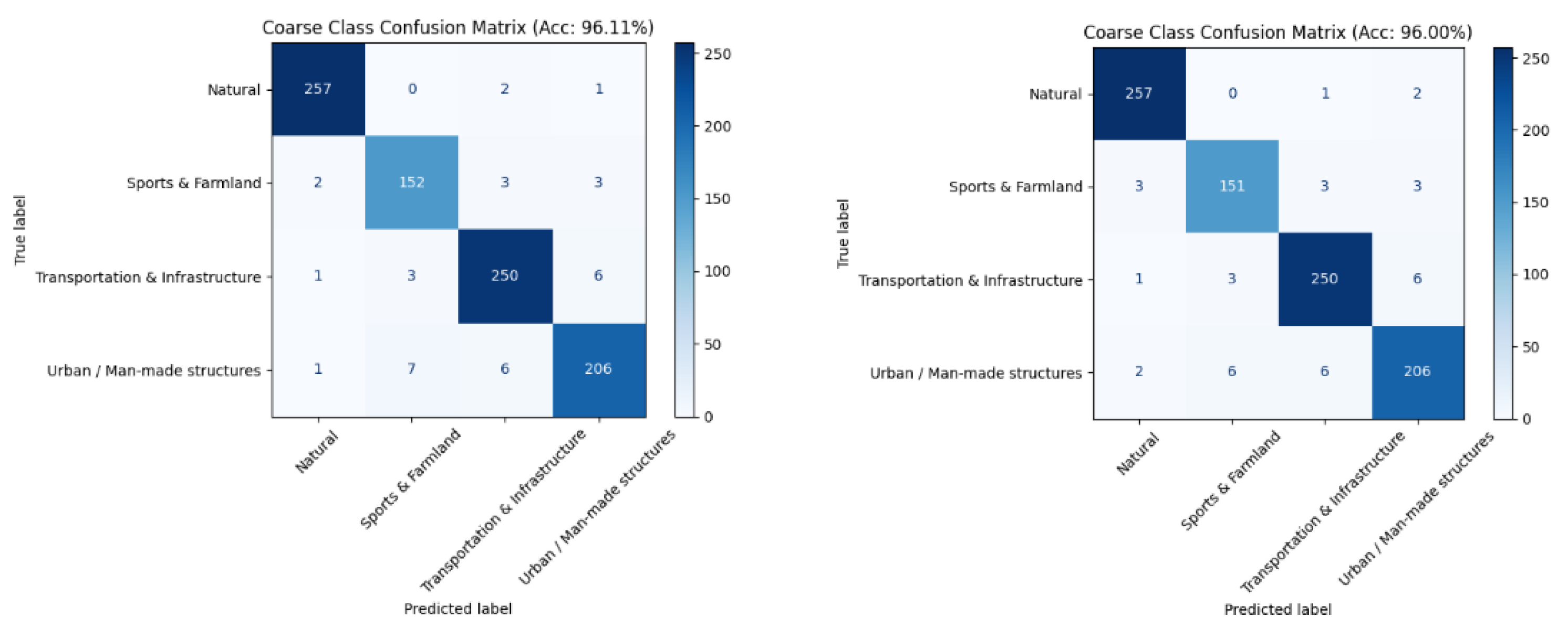
Figure 10.
Top-1 accuracy comparison between LoRA-based tuning and full tuning.
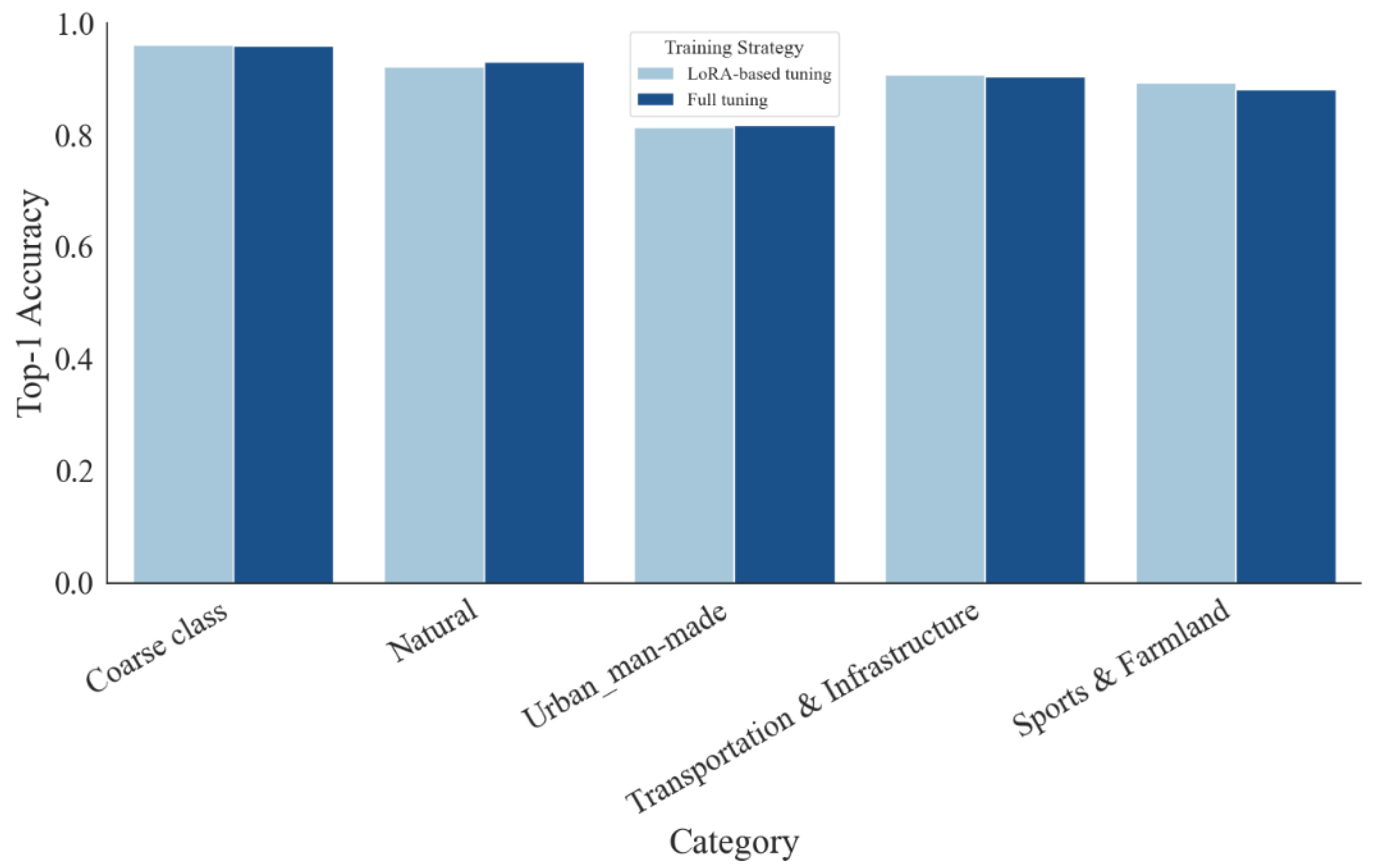
Table 1.
Summary of AID Dataset Versions.
| Version | Key Operations | Details |
|---|---|---|
| Original dataset | 45 classes, 100 images per class; no augmentation data | |
| Data augmentation | Each image transformed with 6 operations: rotate (0°, 90°, 180°, 270°), horizontal flip, vertical flip | |
| Augmentation after split [27] | Training and testing sets split first; augmentation applied only on training set | |
| Class merging data cleaning | Merge semantically similar classes (e.g., church + palace → edifice); remove ambiguous samples | |
| Post-cleaning augmentation | Based on V_3, split into training and testing sets; apply augmentation on training set |
Table 2.
Summary of Prompt Designs (–).
| Version | Main Strategy | Key Features | Output Format |
| Direct classification | Select one category from a list without explanation | Category name only | |
| Coarse-to-fine hierarchical reasoning | Step 1: Coarse classification into 4 major groups; Step 2: Fine-grained classification within selected group; Reasoning required | |Coarse class|Fine class|Reasoning| | |
| Simplified hierar-chical reasoning | Same two-step classification as but with streamlined instructions to reduce cognitive load | |Coarse class|Fine class|Reasoning| |
Table 3.
Top-1 accuracy details of models on different prompt version.
|
Prompt Version |
|||
| Qwen2VL-72B | 29.33% | 52.00% | 51.78% |
| Qwen2.5VL-7B | 90.67% | 96.44% | 96.11% |
Table 4.
Top-1 accuracy details of models based on Qwen2.5 and Qwen2 architectures.
| Model Architecture | Qwen2VL | Qwen2.5VL | Improvement |
| Coarse class | 51.78% | 96.56% | +44.78% |
| Natural | 44.62% | 93.85% | +49.23% |
| Urban / Man-made | 13.64% | 78.64% | +65.00% |
| Transportation & Infrastructure | 18.08% | 91.15% | +73.07% |
| Sports & Farmland | 2.50% | 95.00% | +92.50% |
Table 5.
Top-1 accuracy details of 7B and 72B models based on Qwen2.5 architecture.
| Model Size | 7B | 72B | Improvement |
| Coarse class | 96.11% | 96.56% | +0.45% |
| Natural | 92.31% | 93.85% | +1.54% |
| Urban / Man-made | 81.36% | 78.64% | -2.72% |
| Transportation & Infrastructure | 90.77% | 91.15% | +0.38% |
| Sports & Farmland | 89.38% | 95.00% | +5.62% |
Table 6.
Top-1 accuracy details of LoRA-based tuning and full tuning.
| Training Strategy | LoRA | Full | Improvement |
| Coarse class | 96.11% | 96.00% | -0.11% |
| Natural | 92.31% | 93.08% | +0.77% |
| Urban / Man-made | 81.36% | 81.82% | +0.46% |
| Transportation & Infrastructure | 90.77% | 90.38% | -0.39% |
| Sports & Farmland | 89.38% | 88.12% | -1.26% |
Table 7.
CNN vs. VLM w/ hierarchical prompting on AID- (same split/augment).
| Model | Trainable Params (M) | Peak Mem (GB) | Top-1 Accuracy (%) | Macro-F1 (%) |
| ResNet-50 (ImageNet) | 23.60 | 3.139 | 90.67 | 90.46 |
| MobileNetV2 (ImageNet) | 2.282 | 2.626 | 89.78 | 89.81 |
| EfficientNet-B0 (ImageNet) | 4.065 | 2.968 | 91.11 | 91.09 |
| Qwen2.5VL-7B+LoRA+HPE | 8.39 | 14.00 | 91.33 | 91.32 |
Table 8.
Accuracy (Top-1 / Macro-F1) (%) vs. labeled fraction on AID-.
| Labeled (%) | ResNet-50 | MobileNetV2 | EfficientNet-B0 | Qwen2.5VL-7B + LoRA |
| 1% | 27.89 / 26.25 | 53.44 / 53.46 | 29.00 / 28.81 | 81.44 / 82.63 |
| 5% | 49.33 / 47.63 | 67.00 / 65.94 | 53.67 / 53.02 | 87.22 / 87.90 |
| 10% | 69.44 / 69.44 | 81.11 / 80.98 | 75.00 / 74.51 | 85.22 / 84.92 |
| 25% | 84.33 / 84.22 | 90.00 / 89.94 | 86.22 / 86.13 | 87.11 / 87.04 |
Table 9.
Few-shot LoRA vs Zero-shot in cross-domain.
| Dataset | Few-shot LoRA | Zero-shot | ||
| Coarse Top-1 | Coarse F1 | Coarse Top-1 | Coarse F1 | |
| AID- | 97.78 | 97.67 | - | - |
| UCM | 95.70 | 95.55 | 87.20 | 87.04 |
| WHU | 96.81 | 95.92 | 93.90 | 91.98 |
| RSSCN7 | 82.37 | 62.64 | 74.07 | 28.11 |
Disclaimer/Publisher’s Note: The statements, opinions and data contained in all publications are solely those of the individual author(s) and contributor(s) and not of MDPI and/or the editor(s). MDPI and/or the editor(s) disclaim responsibility for any injury to people or property resulting from any ideas, methods, instructions or products referred to in the content. |
© 2025 by the authors. Licensee MDPI, Basel, Switzerland. This article is an open access article distributed under the terms and conditions of the Creative Commons Attribution (CC BY) license (http://creativecommons.org/licenses/by/4.0/).
Copyright: This open access article is published under a Creative Commons CC BY 4.0 license, which permit the free download, distribution, and reuse, provided that the author and preprint are cited in any reuse.


