A Second-Order Upper Bound on the Expected Value of a Convex Function - Revisited - a Geometric Proof

1. Introduction

The paper presents a new proof of a second-order upper bound on the expected value of a convex function of a random variable; see, e.g. [1], for the algebraic proof of the bound. The paper presents a geometric proof of the same bound. The bound is a deterministically valid bound-based approximation. The bound falls into the realm of the safe side of stochastic programming bounds and approximations.

When designing an optimization model that accounts for the uncertainty of input data described by probability distributions, it often happens that the probability distributions themselves that define the uncertainty are only partially known.

This leads to the need to use approximations based on lower and upper bounds, which are valid only when limited information about the probability distributions is available. The computational complexity of an optimization model also requires the availability of such specialized techniques for a fast solution.

The development of upper bound approximations used in stochastic programming originates in the 1950’s with work of Edmundson [2] and Madansky [3]. This early work provides a first-order upper bound on the expected value of a convex function of a random variable. A second-order upper bound is derived from Dulá [4] on infinite support of the underlying random variable. In the univariate case, this bound is refined on a finite support in [1], where it is called the Dula bound on a finite support (DBFS). The derivation therein uses a relaxation of the Generalized Moment Problem (GMP); see, e.g., [5] for an overview of GMP.

The remainder of this paper is organized as follows. In Section II, we present a new proof of DBFS based on geometric construction. Section III presents our empirical results with respect to 29 crypto currency ETFs (Exchange Traded Funds) over an 18-month period on the NASDAQ market. In Section IV, we conclude the paper and provide directions for future research and applications.

2. A Geometric Construction

We consider a convex function $f\left(x\right)$ defined on a finite interval $[a,b]$, and a non-degenerate random variable $\xi$ that has support contained in $[a,b]$. The random variable has an unknown probability distribution with known information available only for the first two moments: expectation $\mu =\mathbb{E}\left[\xi \right]$ and the second power moment $m_2=\mathbb{E}\left[{\xi }^2\right]$. Evidently, the first moment satisfies the condition $a\le \mu \le b$ and the variance ${\sigma }^2=m_2-{\mu }^2$ satisfies the condition ${\sigma }^2\le (\mu -a)(b-\mu )$.

The goal is to prove that the expectation $\mathbb{E}\left[f\right(\xi \left)\right]$ is bounded by the upper bound $U{B}_2$ derived in [1]. The expectation is taken with respect to the unknown probability distribution, which is followed by the random variable $\xi$ that has only limited probability moment information given by $\mu$ and $\sigma$. For this, we bound the function $f\left(x\right)$, from above, for every x in $[a,b]$ in two steps: (i) first, by a piecewise linear function, called $PWL\left(x\right)$, and (ii) second, the function $PWL$ is bounded above by a quadratic function called $q\left(x\right)$.

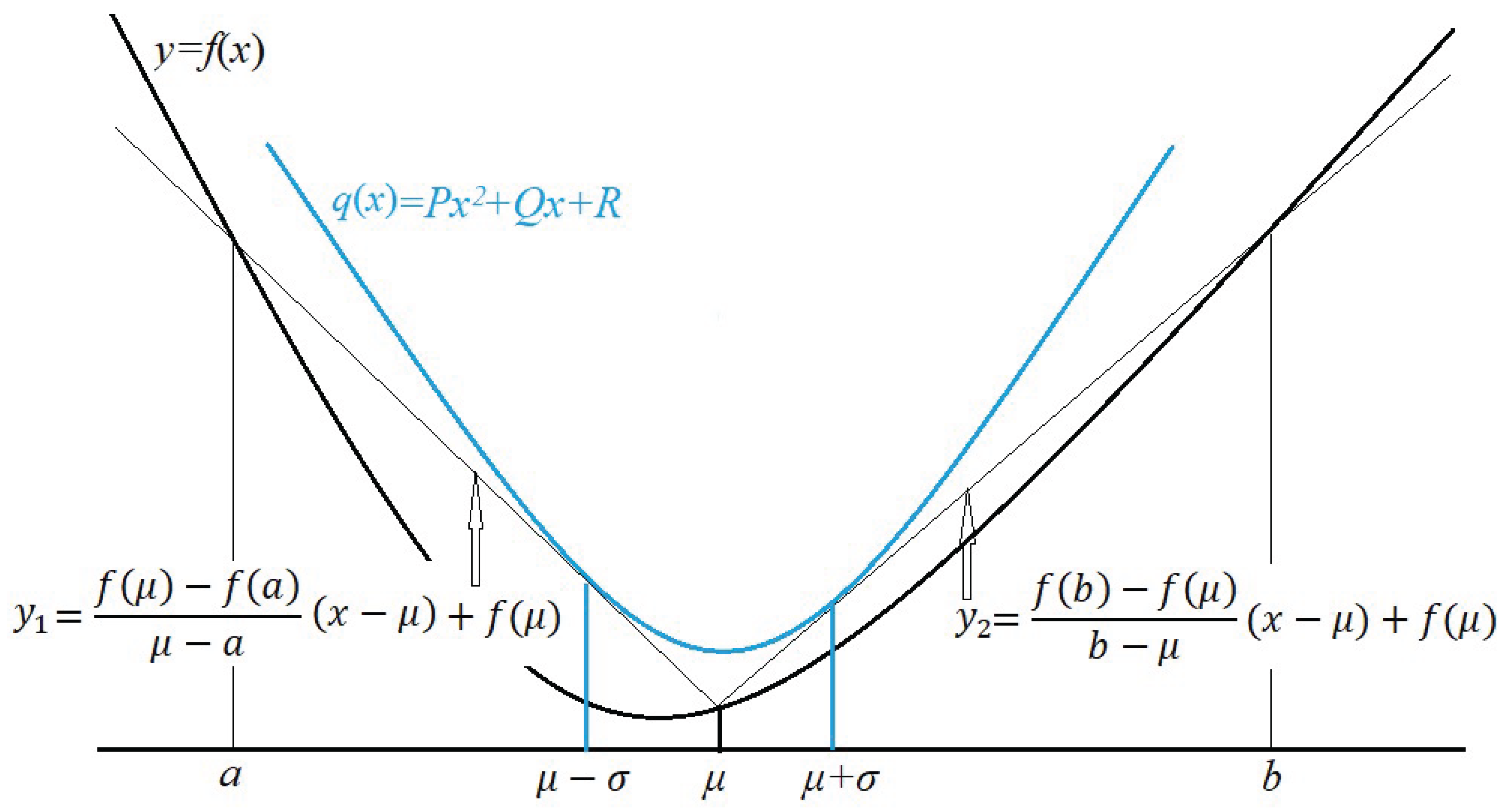
For our geometric construction, we present the analytical formulas for the functions $PWL\left(x\right)$ and $q\left(x\right)$ involved in the two-step bounding procedure. We consider two secant lines to the graph of $f\left(x\right)$ which are denoted as $y_1\left(x\right)$ and $y_2\left(x\right)$ passing through the pairs of points $(a,f(a\left)\right)$, $(\mu ,f(\mu \left)\right)$ and $(\mu ,f(\mu \left)\right)$, $(b,f(b\left)\right)$, respectively, see Figure 1. Thus, $PWL\left(x\right)$ is defined as the greater of the two straight lines $y_1\left(x\right)$ and $y_2\left(x\right)$.

$$\begin{array}{c}\hfill PWL\left(x\right)=max(y_1\left(x\right),y_2\left(x\right)),\mathrm{for}x\in [a,b].\end{array}$$

Specifically,

$$\begin{array}{c}\hfill PWL\left(x\right)=\left\{\begin{array}{cc}{y}_1\left(x\right)={\displaystyle \frac{f\left(\mu \right)-f\left(a\right)}{\mu -a}}(x-\mu )+f\left(\mu \right)\hfill & \mathrm{if}x\in [a,\mu ]\hfill \\ y_2\left(x\right)={\displaystyle \frac{f\left(b\right)-f\left(\mu \right)}{b-\mu }}(x-\mu )+f\left(\mu \right)\hfill & \mathrm{if}x\in [\mu ,b]\hfill \end{array}\right.\end{array}$$

(1)

The quadratic function $q\left(x\right)=P{x}^2+Qx+R$ bounds $PWL\left(x\right)$ from above by the following construction. The parabola $q\left(x\right)$ passes through the pair of points $(\mu -\sigma ,y_1(\mu -\sigma ))$ and $(\mu +\sigma ,y_2(\mu +\sigma ))$. Furthermore, the quadratic function $q\left(x\right)$ has the straight lines $y_1$ and $y_2$ as tangent lines at the same pair of passing points $(\mu -\sigma ,y_1(\mu -\sigma ))$ and $(\mu +\sigma ,y_2(\mu +\sigma ))$, respectively. The parabola $q\left(x\right)$ may seem overdetermined because it must satisfy 4 conditions, while it only has 3 coefficients $P,Q$ and R to be determined. However, in the following theorem we show that such a parabola exists. Basically, this is a standard fact for a parabola and its pair of tangent lines, which can be checked online. The fact states that two tangent lines to a parabola intersect at a point with the abscissa, which is the midpoint of the abscissas of the two tangent points.

Theorem 1.

There exist coefficients $P,Q$ and R such that the quadratic function $q\left(x\right)=P{x}^2+Qx+R$ goes through the points $(\mu -\sigma ,y_1(\mu -\sigma ))$ and $(\mu +\sigma ,y_2(\mu +\sigma ))$, that is, $q\left(x\right)$ satisfies the pair of equations

$$\begin{array}{cc}\hfill P{(\mu -\sigma )}^2+Q(\mu -\sigma )+R=& {\displaystyle \frac{f\left(\mu \right)-f\left(a\right)}{\mu -a}}(-\sigma )+f\left(\mu \right)\hfill \end{array}$$

(2)

$$\begin{array}{cc}\hfill P{(\mu +\sigma )}^2+Q(\mu +\sigma )+R=& {\displaystyle \frac{f\left(b\right)-f\left(\mu \right)}{b-\mu }}(+\sigma )+f\left(\mu \right)\hfill \end{array}$$

(3)

and, moreover, the quadratic function $q\left(x\right)$ has the straight lines $y_1$ and $y_2$ as tangent lines, that is, $q\left(x\right)$ satisfies the pair of equations

$$\begin{array}{cc}\hfill 2P(\mu -\sigma )+Q=& {\displaystyle \frac{f\left(\mu \right)-f\left(a\right)}{\mu -a}}\hfill \end{array}$$

(4)

$$\begin{array}{cc}\hfill 2P(\mu +\sigma )+Q=& {\displaystyle \frac{f\left(b\right)-f\left(\mu \right)}{b-\mu }}\hfill \end{array}$$

(5)

However, the “overdetermined” linear system with the above 4 equations and 3 variables has the following solution

$$\begin{array}{cc}\hfill P=& {\displaystyle \frac{S^{-}}{4\sigma }}\hfill \\ \hfill Q=& {\displaystyle \frac{S^{+}}{2}}-{\displaystyle \frac{\mu S^{-}}{2\sigma }}\hfill \\ \hfill R=& {\displaystyle \frac{\sigma }{2}}{S}^{-}+f\left(\mu \right)-P{m}_2-Q\mu \hfill \end{array}$$

where the following notations are applied.

$$\begin{array}{cc}\hfill S^{-}=& {\displaystyle \frac{f\left(b\right)-f\left(\mu \right)}{b-\mu }}-{\displaystyle \frac{f\left(\mu \right)-f\left(a\right)}{\mu -a}}\hfill \\ \hfill S^{+}=& {\displaystyle \frac{f\left(b\right)-f\left(\mu \right)}{b-\mu }}+{\displaystyle \frac{f\left(\mu \right)-f\left(a\right)}{\mu -a}}\hfill \end{array}$$

Proof. 

For solving the linear system with 4 equations (2) - (5) and 3 variables $P,Q$ and R, we note that we can readily solve equations (4) and (5) for P and Q, because this is a trivial system with 2 variables and 2 equations. Then we find the desired value for the third variable R from either (2) or (3), which completes the proof. □ □

Theorem 1 provides the bai for an upper bound on expectation $\mathbb{E}\left[f\right(\xi \left)\right]$. We note that

$$f\left(x\right)\le PWL\left(x\right)\le q\left(x\right),\mathrm{for}\mathrm{every}x\in [a,b].$$

(6)

Based on the chain of inequalities (6) we conclude that with probability one (w.p.1) we have

$$f\left(\xi \right)\le PWL\left(\xi \right)\le q\left(\xi \right),\mathrm{w}.\mathrm{p}.1.$$

(7)

Taking the expectation in (7) yields the desired upper bound.

$$\mathbb{E}\left[f\left(\xi \right)\right]\le \mathbb{E}\left[q\left(\xi \right)\right]\equiv U{B}_2,$$

(8)

where the upper bound $U{B}_2$, a.k.a. DBFS, is derived in [1] as

$$U{B}_2={\displaystyle \frac{\sigma }{2(m_1-a)}}f\left(a\right)+{\displaystyle \frac{\sigma }{2(b-m_1)}}f\left(b\right)+\left(1-{\displaystyle \frac{\sigma (b-a)}{2(m_1-a)(b-m_1)}}f\left(\mu \right)\right)$$

(9)

The equality $E\left[q\left(\xi \right)\right]=U{B}_2$ can be verified by standard algebraic manipulation.

Although the upper bound (8), developed in the paper by a geometric construction, considers the case of a uni-variate random variable $\xi$, applications can be made when $\xi$ itself depends in a functional form on other random variables. One such case is presented in the next section.

3. Numerical Results

We consider a portfolio optimization problem that minimizes the expected shortfall of portfolio return. The portfolio return is an uni-variate random variable that depends on the assets constituting the portfolio. Unfavorable small values of portfolio returns are penalized by minimizing the expectation of the portfolio return shortfall function.

The portfolio return $r_p={\mathbf{x}}^{\top }\xi$ is represented by the inner product of the decision vector $\mathbf{x}=(x_1,...,x_m)$ containing the trading signals $x_i$’s for each asset and the vector of random assets returns $\xi =({\xi }_1,...,{\xi }_m)$, where m is the number of assets in the portfolio. For the expected portfolio return shortfall, we consider a benchmark-based convex function (convexity with respect to $r_p$) of the following standard form:

$$u\left({\mathbf{x}}^{\top }\xi \right)={[{\mu }_b-{\mathbf{x}}^{\top }\xi ]}^{+},$$

Minimization of the expectation $\mathbb{E}\left[u\left(r_p\right)\right]$ reduces the risk of portfolio return falling short of a benchmark target return specified by ${\mu }_b$. The function $u\left(r_p\right)$ is non-differentiable, so we approximate its expectation by the upper bound $U{B}_2$ in (9), which is a smooth function with respect to the decision vector.

The trading signals $\mathbf{x}=(x_1,...,x_m)$ for each asset in the portfolio come from the minimization of $U{B}_2\left(u\left(r_p\right)\right)$. To apply the upper bound approximation $U{B}_2$, we assume that the vector of asset returns $\xi$ has bounded support contained in a finite interval $[a,b]$. In particular, we assume that $a_i\le {\xi }_i\le b_i$, w.p.1., (i.e., with probability one) for every asset $i=1,...,m$ and thus

$$0\le a=\underset{1\le i\le m}{min}{a}_i\le r_p\left(\mathbf{x}\right)\le \underset{1\le i\le m}{max}{b}_i=b.$$

The use of $U{B}_2$ requires calculation of the portfolio mean return and portfolio variance $m_1=\mathbb{E}\left(r_p\right)=\mathbb{E}\left({\mathbf{x}}^{\top }\xi \right)={\mathbf{x}}^{\top }\mu$ and ${\sigma }^2=Var\left(r_p\right)={\mathbf{x}}^{\top }\Sigma \mathbf{x}$, respectively. After the minimization of the upper bounding approximation $U{B}_2$ of the expected portfolio return shortfall, we “trade” the optimal portfolio signals $\mathbf{x}$. To account for the available budget for the traded portfolio, in other words, to take into account the buying power of the portfolio, the optimal trading signals $\mathbf{x}$ are normalized so that the sum of absolute values of the short and long signals is exactly one. The formula $x_i/$sum$\left(abs\right(\mathbf{x}\left)\right)$ is applied for the normalization of every trading signal, i.e., to achieve desired portfolio buying power.

The asset returns, in $\xi$, are daily returns from market-open to market-close prices for the assets constituting the portfolio. In our numerical application, we use daily open and closing prices for 29 crypto currencies, shown in Table 2, for 1.5 years beginning from 1/11/2024 until 8/29/2025. Statistical estimates for the first two probability moments $\mu$ and $\Sigma$, the asset mean returns and variance-covariance matrix, respectively, come from using the last 42 trading/ working days (two calendar months) of daily returns. Then, on the next day, we trade (out-of-sample) with market-on-open orders, and at the end of the trading day, we liquidate all positions with market-on-close orders. In this way, we perform out-of-sample statistical testing for the profit-and-loss (PnL) generated by our trading signals.

Table 1 displays the sample statistics for the PnL for the optimal daily trading signals obtained by minimizing the DBFS bound on the expected portfolio return shortfall. We note that the DBFS defining expression $U{B}_2$ is a smooth function, while the expected shortfall is a non-differentiable function. Hence, minimizing DBFS is a favorable choice in this case.

Table 1. Performance statistics for the portfolio trading signals that minimize the DBFS upper bounding approximation of the expected portfolio shortfall function on daily basis for the 29 crypto currency ETFs shown in Table 2. Performance statistics are estimated based on 368 out-of-sample daily realized gains and losses from 3/13/2024 to 8/29/2025.

Statistics	Daily PnL	with Leverage ratio 4:1
Annual return in %	2.9	11.55
Annual st.dev. in %	0.7	2.85
Sharpe ratio at 0%	4.1	4.06
Best Month in %	0.75	3.01
Worst Month in %	-0.16	-0.62
Ave. Gain Mo. in %	0.28	1.13
Ave. Loss Mo. in %	-0.09	-0.39
Percent Up Months	89	89

Table 1. Performance statistics for the portfolio trading signals that minimize the DBFS upper bounding approximation of the expected portfolio shortfall function on daily basis for the 29 crypto currency ETFs shown in Table 2. Performance statistics are estimated based on 368 out-of-sample daily realized gains and losses from 3/13/2024 to 8/29/2025.

Statistics	Daily PnL	with Leverage ratio 4:1
Annual return in %	2.9	11.55
Annual st.dev. in %	0.7	2.85
Sharpe ratio at 0%	4.1	4.06
Best Month in %	0.75	3.01
Worst Month in %	-0.16	-0.62
Ave. Gain Mo. in %	0.28	1.13
Ave. Loss Mo. in %	-0.09	-0.39
Percent Up Months	89	89

The summary statistics in Table 1 do not include any transaction costs and fees on the 29 crypto currency ETFs. However, the Sharpe ratio is higher, higher than the usual benchmark of 3 units for such a ratio. Thus, it is good enough to allow for higher leverage, which increases both the annual return and risk. However, the risk represented by the annualized standard deviation is still acceptably small, which is seen in the last column of the summary statistics table.

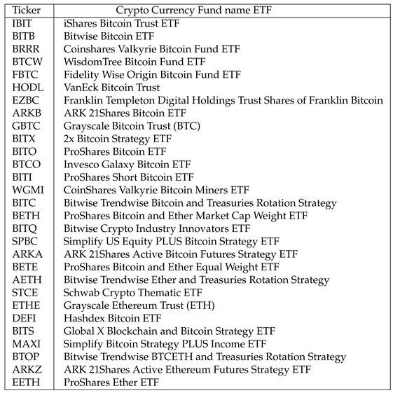
Table 2. Table containing 29 crypto currency ETFs (Exchange Traded Funds) from the NASDAQ market - Ticker for stock listings (in the 1st column) and actual Fund name (in the 2nd column). Daily open and close prices for the 29 crypto currency ETFs are collected from 2024/1/11 until 2025/8/29. The starting date comes from the fact that this is the time when most of the crypto currency ETFs were created, accepted and included in the stock listings on the NASDAQ market.

Ticker	Crypto Currency Fund name ETF
IBIT	iShares Bitcoin Trust ETF
BITB	Bitwise Bitcoin ETF
BRRR	Coinshares Valkyrie Bitcoin Fund ETF
BTCW	WisdomTree Bitcoin Fund ETF
FBTC	Fidelity Wise Origin Bitcoin Fund ETF
HODL	VanEck Bitcoin Trust
EZBC	Franklin Templeton Digital Holdings Trust Shares of Franklin Bitcoin
ARKB	ARK 21Shares Bitcoin ETF
GBTC	Grayscale Bitcoin Trust (BTC)
BITX	2x Bitcoin Strategy ETF
BITO	ProShares Bitcoin ETF
BTCO	Invesco Galaxy Bitcoin ETF
BITI	ProShares Short Bitcoin ETF
WGMI	CoinShares Valkyrie Bitcoin Miners ETF
BITC	Bitwise Trendwise Bitcoin and Treasuries Rotation Strategy
BETH	ProShares Bitcoin and Ether Market Cap Weight ETF
BITQ	Bitwise Crypto Industry Innovators ETF
SPBC	Simplify US Equity PLUS Bitcoin Strategy ETF
ARKA	ARK 21Shares Active Bitcoin Futures Strategy ETF
BETE	ProShares Bitcoin and Ether Equal Weight ETF
AETH	Bitwise Trendwise Ether and Treasuries Rotation Strategy
STCE	Schwab Crypto Thematic ETF
ETHE	Grayscale Ethereum Trust (ETH)
DEFI	Hashdex Bitcoin ETF
BITS	Global X Blockchain and Bitcoin Strategy ETF
MAXI	Simplify Bitcoin Strategy PLUS Income ETF
BTOP	Bitwise Trendwise BTCETH and Treasuries Rotation Strategy
ARKZ	ARK 21Shares Active Ethereum Futures Strategy ETF
EETH	ProShares Ether ETF

Table 2. Table containing 29 crypto currency ETFs (Exchange Traded Funds) from the NASDAQ market - Ticker for stock listings (in the 1st column) and actual Fund name (in the 2nd column). Daily open and close prices for the 29 crypto currency ETFs are collected from 2024/1/11 until 2025/8/29. The starting date comes from the fact that this is the time when most of the crypto currency ETFs were created, accepted and included in the stock listings on the NASDAQ market.

Ticker	Crypto Currency Fund name ETF
IBIT	iShares Bitcoin Trust ETF
BITB	Bitwise Bitcoin ETF
BRRR	Coinshares Valkyrie Bitcoin Fund ETF
BTCW	WisdomTree Bitcoin Fund ETF
FBTC	Fidelity Wise Origin Bitcoin Fund ETF
HODL	VanEck Bitcoin Trust
EZBC	Franklin Templeton Digital Holdings Trust Shares of Franklin Bitcoin
ARKB	ARK 21Shares Bitcoin ETF
GBTC	Grayscale Bitcoin Trust (BTC)
BITX	2x Bitcoin Strategy ETF
BITO	ProShares Bitcoin ETF
BTCO	Invesco Galaxy Bitcoin ETF
BITI	ProShares Short Bitcoin ETF
WGMI	CoinShares Valkyrie Bitcoin Miners ETF
BITC	Bitwise Trendwise Bitcoin and Treasuries Rotation Strategy
BETH	ProShares Bitcoin and Ether Market Cap Weight ETF
BITQ	Bitwise Crypto Industry Innovators ETF
SPBC	Simplify US Equity PLUS Bitcoin Strategy ETF
ARKA	ARK 21Shares Active Bitcoin Futures Strategy ETF
BETE	ProShares Bitcoin and Ether Equal Weight ETF
AETH	Bitwise Trendwise Ether and Treasuries Rotation Strategy
STCE	Schwab Crypto Thematic ETF
ETHE	Grayscale Ethereum Trust (ETH)
DEFI	Hashdex Bitcoin ETF
BITS	Global X Blockchain and Bitcoin Strategy ETF
MAXI	Simplify Bitcoin Strategy PLUS Income ETF
BTOP	Bitwise Trendwise BTCETH and Treasuries Rotation Strategy
ARKZ	ARK 21Shares Active Ethereum Futures Strategy ETF
EETH	ProShares Ether ETF

4. Conclusion

The paper presents a new proof for a second-order upper bound on the expectation of a convex function of a random variable. The proof is based on geometric construction. The convex function is bounded above by a piece-wise linear function, which is itself bounded above by a parabola. Analytical formulas are derived for these bounding functions. Then the expectation of the parabola is derived. It turns out that the latter expectation coincides with the formula for the Dulá’s bound on finite support.

A numerical application is presented to develop an optimal portfolio with trading signals. The portfolio minimizes the second-order upper bound of the expected portfolio return shortfall. The out-of-sample performance of the portfolio is analyzed and summarized. The portfolio consists of 29 popular crypto currency ETFs (Exchange Traded Funds) that were recently introduced on the NASDAQ market. Further applications can be done on classical stocks traded on the NASDAQ or NYSE, the New York Stock Exchange.

References

- Dokov, S., Popova, I., Morton, D.,: Efficient Portfolios Computed via Moment-Based Bounding-approximations: Part II - DBFS. In: 2021 International Conference on Information Science and Communications Technologies (ICISCT), IEEE Xplore, . [CrossRef]
- Edmundson, H.P.,: Bounds on the expectation of a convex function of a random variable, Technical report, The Rand Corporation Paper 982, Santa Monica, California, (1957). https://www.rand.org/pubs/papers/P982.html.
- Madansky, A.,: Bounds on the expectation of a convex function of a multivariate random variable, Ann. Math. Stat. 30, pp. 743–746, (1959). [CrossRef]
- Dulá, J.H.,: An upper bound on the expectation of simplicial functions of multivariate random variables, Mathematical Programming, 55, pp. 69–80, (1992). [CrossRef]
- Krein, M.G., Nudelman, A.A.,: The Markov Moment Problem and Extremal Problems, American Mathematical Society, Providence, Rhode, Island (Translations of Mathematical Monographs, 50) (1977). https://bookstore.ams.org/MMONO/50 https://books.google.al/books?id=0BtovQEACAAJ.