
Submitted:
14 October 2025
Posted:
14 October 2025
You are already at the latest version
Abstract
The Two-Measure theory (TMT) has been developing since 1998 and has yielded a number of highly interesting results, including those not realized in traditional field theory models. The most important advantage of TMT as an alternative theory is that, under the conditions under which all classical tests of general relativity are performed, TMT models are able to accurately reproduce Einstein's general relativity. Despite this, TMT is still often perceived as something too exotic to be relevant to reality. In fact, the fundamental idea underlying TMT seems undeniable: if we truly believe in the effectiveness of mathematics in studying nature, we must agree that there must be a correspondence between the fundamental laws of nature and the structure of the mathematical apparatus necessary to adequately describe them. It then turns out that there is no reason to ignore the volume measure existing on the differentiable manifold on which the theory of gravity and matter fields is built. This idea has far-reaching implications. The goals of this paper are: 1) to provide a clear mathematical and conceptual justification for TMT; 2) to collect in a single article some of the main results of TMT obtained over the past 25 years.
Keywords:
alternative theory of gravity
; two-measure theory
; dark energy
; cosmological constant
; K-essence
; phantom dark energy
; neutrino dark energy
; initial conditions for inflation
1. Introduction
What are these two measures? Why the theory of two measures? To answer these questions, let’s begin by analyzing the generally accepted description of gravity. The mathematical structure on the basis of which the action integral is constructed in Einstein’s General Relativity (GR) can be symbolically represented as
In the Palatini formulation of gravity (P’GR), the metric tensor and the (affine) connection are treated as independent variables. As is well known, in the absence of a non-minimal coupling of matter with curvature, the theory of gravity obtained by variation of the original action coincides with Einstein’s GR. However, in the presence of, for example, a non-minimal coupling of a scalar field with a curvature scalar, the solution of the equations obtained by variation with respect to the affine connection leads to connection coefficients with which the covariant derivative of the metric tensor is non-zero. Violation of the metricity condition means that the space-time is non-Riemannian, and to formulate the theory in a Riemannian space-time, it is necessary to perform the corresponding Weyl transformation of the metric tensor. Typically, such a transformation is performed in the original action in such a way as to eliminate the non-minimal coupling of the scalar field with the curvature scalar, and the set of variables used in this case is called the Einstein frame. The mathematical structure on the basis of which the action integral is constructed in P’GR can be symbolically represented as
Considering the formulation of P’GR from the point of view of the applied mathematical apparatus, we inevitably come to the conclusion that we are dealing with a 4-dimensional differentiable manifold at the stages of equipping it with an affine connection and a metric structure (see, for example, [1]).
If we really believe in the effectiveness of mathematics in studying nature, we can go further and agree that there must be a correspondence between the fundamental laws of nature and the structure of the mathematical apparatus necessary for their adequate description. At the same time, we note that among the mathematical objects commonly used in field theories in 4D space-time, there is no the volume form, which can be defined as a 4-form on the 4D differentiable manifold even before equipping it with an affine connection and a metric structure. The appropriate volume element can be constructed by means of 4 scalar functions () defined on the 4D differentiable manifold, as following
After replacing Einstein’s GR with Palatini’s formulation of gravity, the construction of the Two-Measure theory can be seen as the next step in the realization of a clearly formulated idea: all possible degrees of freedom contained in the action should be considered as independent of each other, and all relationships between them appear as a result of applying the principle of least action. For brevity, we will call this approach to constructing a theory "the principle of maximum dynamic independence (PMDI)". The key to this formulation is the word "all" in the expression "all possible degrees of freedom", and we will now discuss what is meant by this. Using as a volume measure in the action integral, according to PMDI, we must consider the functions as degrees of freedom and, therefore, when finding the action extremum, we must perform variations with respect to as well.
Apparently, it is necessary to more carefully analyze the extent to which it is justified to ignore the volume measure of type (1) in the generally accepted approach. After the metric structure is defined on the manifold, if the latter is orientable, can also be chosen as a 4-form to describe the volume measure in the action integral. The possibility of such two alternative choices is based on the fact that under general coordinate transformations with a positive Jacobian (i.e. without changing the orientation of the manifold), the scalar densities and are transformed according to the same rule. The standard approach (see, for example, section 2.8 in ref. [1]) is to use only the volume element , by default assuming that the volume element is redundant. A more detailed argument for this conclusion is given by R. Wald in appendix B2 in ref. [2]. Considering on n-dimensional manifold M the volume element , where the function f is non-vanishing, Wald reasonably notes that "if one is given only the structute of a manifold M, there is no natural choice of volume element". Wald then shows that if a metric is defined on M, then there exists a natural volume element, given by the n-form . Continuing Wald’s analysis, we note that the possibility of treating the volume element as natural exists only because in Einstein’s GR the metric tensor is a dynamic variable, whose variation in the Einstein-Hilbert action leads to Einstein’s equations. The original idea of the TMT might be that including the volume element in the action integral allows us to consider the function f as another variable subject to variation in the action, along with the metric. But this modification of the theory leads to a trivial result: the function f plays the role of a Lagrange multiplier, and the Lagrangian term entering the action with the volume element turns out to be equal to zero. The idea of the TMT makes sense if, following PMDI, we fully exploit the capabilities of a differentiable manifold M. Returning from the n-dimensional manifold to the 4-dimensional one and using four arbitrary functions () (differentiable a sufficient number of times), we can construct a 4-form (1) and consider it as a volume element in the action integral together with the volume element . In this formulation of the theory, varying the functions leads to an equation with a significant dynamic effect. This is the essence of the TMT, and, returning to the analysis of Wald’s argumentation, we see that the volume elements and turn out to be equally natural.
A closer look at the problem when the functions are added to the set of degrees of freedom in action shows that as a result of varying the action, the scalar function in the form of the ratio of volume measures
appears in all equations of motion and plays a decisive role in all new effects of TMT. Bearing in mind that gravity in GR has a geometric nature described by the metric tensor, we will use the term pregeometry for effects caused by the scalar .
The organization of the paper is as folllows. In Section 2 we show that in empty space the solution of the equations of the gravity model with two volume measures lead to the result , i.e. there is no fundamental difference between the volume measures and . However, even in empty space the gravity model with two measures acquires new interesting properties compared to the gravity model with only one measure . In Section 3, we show that in TMT, the physical results depend on orientation of the space-time manifold and, moreover, that the latter arises spontaneously. By analyzing the mathematical differences between the volume measures and , we arrive at a formulation of possible structural properties of the action integral in TMT. An important note regarding the terminology used in this article is also provided at the end of this section. In Section 4, using a toy model as an example, we demonstrate the main features of the TMT and describe in detail the computational procedure in TMT. In Section 5 a class of TMT models that provide quintessence without the need for fine-tuning is described. In Section 6, four TMT models with global scale invariance are considered. These models demonstrate the possibility of solving a number of fundamental problems in gravity and cosmology. A model of dark energy generated by neutrinos without a scalar field is presented in Section 7. The TMT effect, related to a possible connection between the Borde-Guth-Vilenkin theorem and initial conditions for inflation, is discussed in Section 8.
2. The Two-Measure Theory in Empty Space
When constructing models with two volume measures, we assume that the total volume measures in the action integral have the form of linear combinations , in which the constant real coefficients , can be different depending in which term of the Lagrangian density they are present with in the original action.
According to PMDI, the affine connection and metric tensor should be treated as independent degrees of freedom, i.e., one should proceed in the Palatini formulation. Using the definitions , and , let us consider the TMT model in the empty space with the following action
Bearing in mind that the further description of this model will also use redefinitions of the parameters , and the functions (and hence ), we use the tilde to denote them here. Last two terms in (3) have the nature of the vacuum-like terms. If the first term, was present in Einstein’s GR, would be a cosmological constant. The term with was first introduced in ref. [5]. The reason for adding the term with is that the term , which can be expected as the contribution of quantum-gravitational effects to a vacuum-like action, does not contribute to the equations of motion. Therefore, the next in powers of vacuum-like term can be of the form . It is assumed that , and , .
The action includes the following independent variables (and takes into account the effect of pre-geometry): the affine connection , the metric tensor and four scalar functions , (a=1...4), with the help of which the measure density is constructed. By varying the action with respect to scalar functions we get
Since it follows that if
the equality
must be satisfied, where is a constant of integration with the dimension of .
Variation with respect to yields the equation
The condition for compatibility of Equations (6) and (7) is a constraint in the form of the following expression for a constant scalar
As noted above in assertion 1, the latter means that the solution in empty space reveals that the volume measures and differ only by a constant factor. From the constancy of it follows that the variation of leads to an equation whose solution is the equality , where are the Christoffel’s connection coefficients of the metric . This means that spacetime is Riemannian, there is no need for a Weyl transformation and is the Ricci tensor of the spacetime with the metric . Substituting the value of into Equation (7), we obtain Einstein’s equations in empty space
An important novelty of the solution of the TMT model in empty space compared to the convensional theory is that by choosing the constant of integration , it is possible to realize a solution with any TMT-effective cosmological constant . In particular, by choosing , we obtain a solution with and
It is worth paying special attention to the fact that the relations and (10), which play a very important role, do not contain the parameters and . It can be shown that this fact is not accidental. To do this, we rewrite the action in empty space (3) using the following redefinitions: , , , . As a result, the action (3) takes the form
It is worth noting that the presence of vacuum-like terms violates the symmetry . By acting with (11) in the same way as we did with (3), instead of (6) we first get
where and is the integration constant. Then it follows that
Again, by choosing the integration constant , we can implement a solution with any TMT-effective cosmological constant . In particular, by choosing , we obtain a solution with and .
3. Some Additional Mathematical Aspects Taken into Account in TMT
Before moving on to the study of specific models, it is necessary to return to the mathematical aspects of the existence of the two volume measures and and take into account the important differences between them. The density of the volume measure is positive-definite and the volume measure is defined if the manifold is oriented. But , which plays the role of the density of the volume measure , is generally sign-indefinite. Moreover, the sign of the 4-form determines the sign of the orientation of the manifold (for more details see, for example, [3]). Therefore, using linear combinations as a total volume measures in constructing the terms of the primordial action, we leave the sign of the space-time orientation undefined. And only as a result of choosing a solution to the equations of motion, the sign of is fixed, and, therefore, the sign of the orientation. To understand how this effect occurs, let’s return to the simplest example in empty space described by Equations (13) and (14) (how this happens in the presence of matter we will see later in this paper). To obtain a solution with , we chose the integration constant and as a result found that and, therefore, . However, we could have chosen , which also ensures . But with such a choice, the constraint (13) leads to and, therefore, . Hence, changing the sign of the integration constant , we obtain solutions with opposite sign of the space-time orientation. In essence, we are discovering the TMT-effect of spontaneous restoration of the sign of the space-time orientation, which is one of the effects of pregeometry.
The conclusion that follows from the described TMT effect of spontaneous restoration of space-time orientation is so fundamental that it allows us to formulate in the most concentrated form the main difference between TMT and conventional field theories. In conventional field theories, it is assumed by default that the sign of space-time orientation can be chosen arbitrarily. But in TMT, as we have seen, one of the two possible signs of orientation of the space-time manifold of our Universe is fixed by the choice of the solution of cosmological equations. And since the sign of orientation coincides with the sign of the scalar function , which plays a decisive role in the dynamics of fields, the physical results predicted by TMT turn out to be different for different signs of the space-time orientation.
To construct the action in the presence of matter, we take the action in empty space (11) as the gravitational term, to which the matter terms are added. As matter, we can consider different types of models, and, compared to conventional models, the whole novelty in the context of TMT is the possibility of choosing the coefficients and () in the volume elements in each i-th term of the Lagrangian density.
Since the original action does not imply the existence of a definite space-time orientation, and also because of the the sign-indefinitness of , when constructing the original action terms using linear combinations of and , it should be assumed that the coefficients in front of in the total volume measures can be positive as well as negative. That is, assuming , , the total volume measures can have the form . This finding is a direct consequence of the fact that the original action structure takes pre-geometry into account to a large extent, and this is important for achieving the main results that will be presented in this review. In the following sections, using examples of specific models, we will consider how the above-described features of TMT manifest themselves. But before that, one more remark, more of a technical nature, needs to be made. As follows from the above analysis, the general form of the i-th term of the Lagrangian density is . Since the functions have already been redefined to obtain the gravitational term (11) of the action, to eliminate the coefficient , we can factor it out of the brackets and absorb it by redefining either the model parameters or the fields in . As a result, the i-th term of the Lagrangian density takes the form , where and is obtained from the mentioned redefinitions in . This is the form in which all Lagrangian density terms in TMT models will be used in what follows.
An important note regarding the terminology used in what follows. In models of the "conventional" theory, the original action contains a single volume element . In conventional alternative gravity models, the original action differs from the Einstein-Hilbert action only in the form of the Lagrangian, for example, the presence of a non-minimal coupling with curvature. The transformation to the Einstein frame, which in conventional theories is carried out in the original action, simply changes the set of variables used to describe the theory, but does not change the theory itself. In TMT, the main difference is that, along with the volume measure , the original action contains the volume measure , although a modification of the Lagrangian is also possible. Therefore, the original TMT action differs from the Einstein-Hilbert action in the form of the Lagrangian density, and to bring the TMT action to the Einstein frame, the conformal transformation must exclude from the gravitational term of the action not only the non-minimal coupling, but also . In a theory obtained in this way, the constraint determining cannot arise, that is, by acting in this way we would be dealing with a different theory. It is therefore incorrect to use the term "Jordan frame" in the usual sense for the set of variables in the original action of TMT. To emphasize this distinction, in what follows we will use the terms "primordial variables", "primordial model parameters", "primordial potential", "primordial Lagrangian" and "primordial action" instead of "variables in the original frame", "original model parameters", "original potential", "original Lagrangian" and "original action".
In conclusion of this section, it should be noted that in addition to the ideas for constructing TMT described above, there is a wide class of models that use more than one non-canonical form of space-time volume. For an overview of these modified gravity theories and their applications in cosmology, see article [4] and the references therein.
4. TMT Procedure Using a Toy Model as an Example
The first scalar field TMT models in which the primordial action contains both the volume element and were studied in refs. [5,6,7]. To become familiar with the procedure for deriving equations and their initial analysis in TMT, it is useful to start with a toy model as a simple example. To simplify the TMT structure as much as possible, we restrict ourselves to a model in which the Lagrangian of the field enters the initial TMT action with the same volume element as in the gravitational term in Equation (11). Thus, we choose the primordial action in the form
where the choice of the potential will be discussed later.
Let’s start by varying the action with respect to scalar functions . Similar to what was in Section 2, we get
where . Since it follows that if
the equality
must be satisfied, where is a constant of integration with the dimension of .
Variation of the action with respect to yields the equation
Using the trace of Equation (19) one can eliminate the term from Equation (18). As a result, we come to the conclusion that for these equations to be consistent, it is necessary that an algebraic constraint be satisfied that defines scalar as a function locally dependent on :
Variation of the affine connection yields the equations solution of which has the following form
where are the Christoffel’s connection coefficients of the metric and
If the metricity condition does not hold and consequently geometry of the space-time with the metric is generically non-Riemannian. In what follows we will completely ignore a possibility to incorporate the torsion tensor, which could be an additional source for the space-time to be different from Riemannian. It is easy to see that the transformation of the metric
turns the affine connection into the Christoffel connection coefficients of the metric and the space-time turns into (pseudo) Riemannian.
Gravitational Equation (19) expressed in terms of the metric take the canonical GR form
with the same Newton constant as in the original frame. Here and are the Ricci tensor and the scalar curvature of the metric , respectively. Therefore, gravity becomes canonical, and the set of dynamical variables using the metric can be called the Einstein frame. on the right side of the Einstein Equation (24) is the TMT-effective energy-momentum tensor
and
is the -dependent form of the TMT-effective potential. To avoid confusion, it should be noted that the use of the term "TMT-effective potential" has nothing to do with the effective potential obtained taking into account quantum corrections. The terms "TMT-effective energy-momentum tensor" and "TMT-effective potential" are used to denote the energy-momentum tensor and potential that appear in the equations of motion after performing all the steps of the TMT procedure described above, which begins with varying the primordial TMT action and ends with the transition to the Einstein frame in the equations of motion. It is very important to note that the application of the least action principle in the Palatini formalism does not lead to a differential equation for and therefore ζ is not a dynamical variable. Substituting given by the constraint (20) into (26) and assuming, as in Section 2, and , we find the TMT-effective potential of the field in the following form
which still contains the integration constant .
Just as was done in the Section 2, the desired value of the TMT-effective cosmological constant (CC) can be found by fixing a certain value of . To do this, we first obtain the field equation. By varying the action (15) with respect to with subsequent transition (23) to the Einstein frame, we obtain
where .
Note that instead of the system of the Einstein Equation (24) with the energy-momentum tensor (25) and the field -Equation (28), it is much more convenient to work with the TMT-effective action, the variation of which gives these equations. As usual, if , the energy-momentum tensor can be rewritten in the form of a perfect fluid. Then the pressure density plays the role of the matter Lagrangian in the TMT-effective action, and we arrive at the TMT-effective action
with the following TMT-effective Lagrangian
The idea of working with TMT-effective action and TMT-effective Lagrangian will be useful in this paper when exploring more complex TMT models.
Proceeding with the simplest toy model, we choose the original potential . Then from Equation (28) it follows that the vacuum of the classical field is achieved at . The value of at gives us the following equation describing the dependence of the CC on the integration constant :
Thus, the model predicts two vacuum states with that differ in the sign of in the vacuum and, consequently, in the sign of the corresponding values of .
A solution (18) of Equation (16) exists under the condition , Equation (17), i.e, only if or only if . Therefore, only those solutions of the system of equations are valid for which the corresponding is sign-definite, since Equation (16) is one of the equations of the system. It should be noted here that, as usual, by default we assume that the original metric in the primordial action is regular, that is . Therefore, the validity of the solution regarding the fulfillment of the condition on the sign of can be controlled by checking the sign of the scalar . In other words, only those cosmological solutions (together with their initial conditions and the vacuum states) are valid for which does not change the sign throughout the evolution of the universe. This is another one of the effects of pregeometry.
We found that in the toy model under study there are two vacuum states with and differing in the signs. Therefore, in accordance with the analysis in the previous paragraph, there are two classes of solutions differing in the sign of . Considering that the sign of determines the sign of the orientation of the space-time manifold, we come to the conclusion that the difference between these two classes of solutions is that they are realized on space-time manifolds with opposite orientations.
It seems interesting to find the TMT-effective potentials for the two classes of solutions indicated above. To do this, it is sufficient to substitute the corresponding values and of the integration constant into Formula (27). As a result, we find
Thus, as was the case in the empty space model, we conclude that the physical results predicted by TMT turn out to be different for different signs of spacetime orientation.
5. TMT with Additional, Internal, Symmetry: A Class of TMT Models That Provide Quintessence Without the Need for Fine-Tuning
In this section we will show that in the case where the TMT has additional symmetry, there is a broad class of TMT models that provide the quintessence without the need for fine-tuning. This will be done based on the ideas and results of ref. [8]. The primordial action can be represented in the form
where
There are two differences in the structure of the actions (36) and (15). First, instead of a single primordial potential entering (15) with both volume element and , in the action (36) the primordial potential is split into two: entering with the volume element , and entering with the volume element . Second, the vacuum-like term
is missing from action (36). This choice may be justified if, for some as yet unknown reason (possibly due to a more fundamental theory), the Lagrangian does not depend on the functions from which the volume measure density is constructed. For example, as discussed in paper [5], the presence of such a term in the primordial action may be forbidden if a more fundamental theory requires that the primordial TMT action be invariant, up to a total divergence, under transformations
By performing with action (36)–(38) all the operations that make up the TMT procedure described in detail in Section 4, we arrive at the following results:
where is the integration constant;
the metric tensor in the Einstein frame is defined as in Equation (23);
the Einstein equations (24) with the TMT-effective energy-momentum tensor in the form as in Equation (25) and with the TMT-effective potential
In contrast to convensional gravitational theories where the quintessential potential must be slow decreasing function as , in TMT we have an absolutely new option: the quintessential behaviour of the TMT-effective potential for large enough may be achieved with increasing primordial potentials and . This circumstance enables to avoid both the cosmological constant problem and the problem of the flatness of the quintessential potential.
For illustration of these statements, following ref. [8], we consider two types of models.
5.1. The Inverse Power Low Quintessential Potential
We start from the primordial potentials and which for large enough are dominated by the positive power low functions
with , we obtain the TMT-effective potential which for large enough has the inverse power low form
and does not depend on the integration constant . It should be especially emphasized that adding to the primordial action the term , , which in the convensional gravity models would have the meaning of a cosmological constant, does not affect for sufficiently large . Another particularly interesting case is and, for example, . Then .
Thus starting from the polynomial form of the primordial potentials and with an appropriate choice of the powers and of the leading terms, one can in fact provide a generation of the inverse power low quintessential potential in such a way that neither the cosmological constant problem nor the the problem of the flatness of the quintessential potential do not appear at all.
5.2. The Quintessential Potential of the Exponential Form
If the primordial potentials and are chosen to be exponentially growing as is large enough
where and are positive constants, then for large enough the TMT-effective potential (42) takes the form
The case corresponds to a kind of scale-invariant theory studied by Gundelman[6,7,12,13] and will be considered in the next section. The case is the most interesting from the viewpoint of the quintessence: for , the TMT-effective potential behaves as a decaying exponent
It is noteworthy that, as in case of the inverse power low quintessential potential (45), the asymptotic behavior of does not depend on the integration constant .
It should be noted that if symmetry (40) is broken, then in both types of models considered, adding the term (39) to the action (36) leads to a TMT-effective potential that tends to a constant as .
In [8], by choosing the primordial potentials and as linear combinations of the power and exponential functions of , it was demonstrated that it is possible to obtain the TMT-effective potential , which allows realizing the idea of quintessential inflation [9], and also without the cosmological constant problem. In the range of values corresponding to inflation, is a power function of , which ensures a scenario of chaitic inflation. However, this contradicts the requirement of flatness of the inflationary potential imposed by modern CMB data [10,11].
6. Brief Review of the TMT Models with Global Scale Invariance. Some Results in Cosmology and Gravity
This section provides an opportunity to get acquainted with the main results of a large series of articles investigating models in which the primordial TMT action is invariant with respect to global scale transformations. A common feature of all these models is the absence of the term (39) in the primordial action.
6.1. Scale Invarint Model Originally Developed by E. Guendelman
In series of papers [6,7,12,13], E. Guendelman suggested and studied the scale invariant TMT model with the primordial action
where the primordial potentials are defined by the formulas
The action is invariant under the global scale transformations:
Variation of the primordial action (50) with respect to under the condition yields the equation
The appearance of a nonzero integration constant spontaneously breaks the scale invariance. Continuing to execute all the operations that make up the TMT procedure using the primordial action (50) results in the following:
the metric tensor in the Einstein frame is defined by
the Einstein Equation (24) with the TMT-effective energy-momentum tensor in the form as in Equation (25) and with the TMT-effective potential
This potential has remarkable properties. Firstly, if and , a minimum is achieved at and . This means that the model provides zero cosmological constant without fine tuning. Second, for , has an infinite plateau with height . Therefore, the model can also describe inflation in the slow-roll regime.
Note that since is invariant under the scale transformations (52), (53), in the Einstein frame the latter are reduced to only a shift of the scalar field . In ref.[7] Guendelman showed that Goldstone’s theorem is generally inapplicable in this theory, and, consequently, the Goldstone boson associated with the spontaneous breaking of this symmetry is absent.
These terms cannot be added because they are not invariant with respect to scale transformations (53). But in the model presented in the next subsection, these terms are included in a scale invariant manner.
6.2. K-Essence and Inflation in the Scale Invariant TMT Model
Here a brief review of refs.[14,15] is presented. The TMT model including also the terms contained in (58) is described by the following primordial action
where parameters and are introduced based on the discussion in sectiom Section 3; is a real parameter that is assumed to be positive. Note that the notation used for the constants and differs from that used in Section 4 and Section 5. This action is invariant under the global scale transformations
Note that scalar is invariant under these transformations.
Performing the TMT procedure with action (59) produces the following results:
similar to the model described in Section 6.1, variation of the primordial action (59) with respect to subject to the condition leads to an equation where the appearance of an arbitrary integration constant also breaks the scale invariance;
the constraint defining scalar reads now
where
and the metric tensor in the Einstein frame is defined by
Einstein equations have canonical GR form (19) with the TMT-effective energy-momentum tensor
where the function is defined as following
the -dependent form of the field equation
Similar to what was discussed at the end of the previous subsection, since is invariant under scale transformations (60), spontaneous breaking of scale symmetry in the Einstein frame reduces to spontaneous breaking of shift symmetry . The discussion of the inapplicability of Goldstone’s theorem in this theory, [7], is relevant for this model as well.
If , the TMT-effective energy-momentum tensor (64) can be represented in a form of that of a perfect fluid
with the following energy and pressure densities resulting from Equations (64) and (65) after substituting given by the constraint (61):
Just as the TMT-effective action (29), (30) was constructed for the toy model, in the model under consideration the TMT-effective action, the variation of which leads to the equations written out above, has the form of the k-essence type action [16,17].
where is given by Equation (69). The TMT-effective Lagrangian can be represented in the form
where and depend on only via .
A detailed analysis taking into account the dependence on the model parameters shows that in the initial state of the classical evolution of the universe, the curvature may not have an initial singularity, but its time derivative is singular. This is the type of sudden singularity studied by Barrow [18] on purely kinematic grounds (in the classification of future singularities);
Numerical solutions were found and the phase portrait was studied in detail for different initial conditions. Depending on the choice of regions in the parameter space, the model exhibits various possible outcomes of cosmological dynamics. Among them, it is especially worth noting power law inflation, which, depending on the region in the parameter space (but without fine tuning) ends with a graceful exit either into the state with zero cosmological constant or into the state driven by both a small CC and the field with a quintessence-like potential.
a) In the model with , the following TMT-effective potential of the field results from Equations (65) and (61)
If , , and , then the old cosmological constant problem is solved without any fine-tuning in a manner very similar to that used in refs. [6,7,12,13] and described in Section 6.1. , where , is the minimum of the effective potential, and without any further tuning of parameters and initial conditions. However, as shown in ref. [15], in the model under consideration, the measure density and the primordial metric oscillate around zero during transition to the vacuum state . The latter means that it can only happen with very non-trivial modifications in the understanding of the mathematical foundations of TMT, described in Section 3 and Section 4. The papers [14,15] present a detailed analysis that clarifies how and due to what, contrary to Weinberg’s no-go theorem [19], the old CC problem can be solved in TMT. Namely, in footnote 8 of review [19] S. Weinberg indicates the only exception when the conditions required by the theorem are not satisfied. This is precisely the exception that is implemented in TMT, as shown in section VIII.B of paper [14].
b) There is a wide range of parameters for which the late time Universe undergoes superacceleration: the equation of state is ; w asymptotically, as , tends to from below; asymptotically approaches from below a positive cosmological constant, the smallness of which does not require fine-tuning of the dimensional parameters. In ref.[15] it is shown that the crossing of the phantom divide occurs simultaneously with the change of sign of the total volume measure density in the field kinetic term in the primordial action (59), see Figure 1.
In paper [20] the described model was applied to the closed FRW cosmology and it was shown that it admits stable emerging universe solutions. The transition from the emerging phase to inflation and then to the phase with zero cosmological constant was studied. The spectrum of density perturbations and constraints imposed on the model parameters were also examined.
6.3. Reproducing Einstein’s General Relativity Without the Fifth Force Problem in a Scale-Invariant TMT Model Containing the Dilaton and Dust
The study announced in the title was published in ref.[21]. The model is invariant under the same scale transformations (60) as the model described in Section 6.2. The primordial action of the model differs from the primordial action (59) only by adding the scale invariant action for dust (as a model for matter)
where is an arbitrary parameter. For simplicity we consider the collection of the particles with the same mass parameter m. We assume in addition that do not participate in the scale transformations (60).
In this model we restrict ourselves to a zero temperature gas of particles, i.e. we will assume that for all particles. It is convenient to proceed in the frame where , . Then the particle density is defined by
where and
We will assume that the dimensionless real parameters , and are positive, have the same or very close orders of magnitude
In the absence of matter (dust), the model coincides with the model of Section 6.2 and, hence, all results concerning dark energy coincide with the results discussed in Section 6.2. Therefore, we will focus on the effects caused by dust. The first one concerns the important effect observed when varying with respect to :
The latter equation shows that due to the measure density , the zero temperature gas generically possesses a pressure. As we will see this pressure disappears automatically together with the fifth force as the matter energy density is many orders of magnitude larger then the dark energy density, which is evidently true in all physical phenomena tested experimentally.
The transformation to the Einstein frame (63) causes the transformation of the particle density
Einstein Equation (19) appear now with the TMT-effective energy-momentum tensor with the following components
where the function is given by the formula (65) and notations (62) are used. Function is defined now by the following constraint:
The dilaton field equation in the Einstein frame is as follows
One should now pay attention to the interesting result that the explicit dependence involving the same form of dependence
appears simultaneously in the dust contribution to the pressure (through the last term in Equation (81)), in the r.h.s. of the constraint (82). and in the effective dilaton to dust coupling (see the r.h.s. of Equation (83)). Let us analyze consequences of this wonderful coincidence in the case when the matter energy density (modeled by dust) is much larger than the dilaton contribution to the dark energy density in the space region occupied by this matter. Evidently this is the condition under which all tests of Einstein’s GR, including the question of the fifth force, are fulfilled. Therefore, if this condition is satisfied we will say that the matter is in normal conditions. In conventional (non-TMT) models, the existence of the fifth force becomes a problem precisely under normal conditions. The opposite situation may be realized if the matter is diluted up to a magnitude of the macroscopic energy density comparable with the dilaton contribution to the dark energy density. In this case we say that the matter is in the state of cosmo-low energy physics (CLEP). It is evident that the fifth force acting on the matter in the CLEP state cannot be detected now and in the near future, and therefore does not appear to be a problem. But effects of the CLEP may be important in cosmology, see ref. [22] and the next subsection.
The last terms in Equations (80) and (81), being the matter contributions to the energy density () and the pressure () respectively, generally speaking have the same order of magnitude. But if the dust is in the normal conditions there is a possibility to provide the desirable feature of the dust in GR: it must be pressureless. A detailed analysis of the equations of motion together with the constraint (82) in Appendix A of ref. [21] showed that dust under normal conditions has no pressure, provided that under normal conditions (n.c.) the following equality is satisfied with extremely high accuracy:
Remind that we have assumed . Then , and the transformation (63) and the subsequent equations in the Einstein frame are well defined. Inserting (85) in the last term of Equation (80) we obtain the TMT-effective dust energy density in normal conditions
Substitution of (85) into the rest of the terms of the components of the energy-momentum tensor (80) and (81) gives the dilaton contribution to the energy density and pressure of the dark energy which have the orders of magnitude close to those in the absence of matter case, Equations (68) and (69). The latter statement may be easily checked by using Equations (61), (85) and (76).
Detailed analysis shows that the constraint (82) describes a balance between the pressure of the dust in normal conditions on the one hand and the vacuum energy density on the other hand. This balance is realized due to the condition (85). The most obvious way to verify that there is no fifth force problem under normal matter conditions is to consider the -equation (83) and estimate the Yukawa type coupling constant in the r.h.s. of this equation. In fact, using the constraint (82) and representing the particle density in the form where N is the number of particles in a volume , one can make the following estimation for the effective dilaton to matter coupling "constant" f defined by the Yukawa type interaction term (if we were to invent an effective action whose variation with respect to would result in Equation (83)):
Thus we conclude that the effective coupling "constant" of the dilaton to cold matter (dust) in the normal conditions is of the order of the ratio of the "mass of the vacuum" in the volume occupied by the matter to the Planck mass taken N times. In some sense this result resembles the Archimedes law. At the same time Equation (87) gives us an estimation of the exactness of the condition (85).
6.4. Scale Invariant TMT Model Including Fermions. Neutrino Dark Energy
Considering the model of ref.[14] simplified by fitting and adding fermions, in paper [22] the scale invariant model including fermions was studied. In this section we present the main results of [22] with some additional analysis. Omitting the gauge field contribution, the corresponding primordial action is with the Lagrangian density
where () is the general notation for the primordial fermion fields N and E (say, the primordial neutrino and the primordial electron); and are the mass parameters; , is the scalar curvature; and are the vierbein and spin-connection; and . Constants are non specified dimensionless real parameters and we will only assume that they have close orders of magnitude
The formulation of the primordial action(88) in the Palatini formalism means that vierbein and spin-connection are considered as independent degrees of freedom.
The action (88) is invariant under the global scale transformations:
where , and ; scalar is invariant under these transformations.
Similar to the models of the previous subsections, variation of the primordial action (88) with respect to subject to the condition leads to an equation where the appearance of an arbitrary integration constant also breaks the scale invariance. All other equations of motion resulting from (88) in the Palatini formalism contain terms proportional to that makes the space-time non-Riemannian and equations of motion - non canonical. However, with the new set of variables ( remains unchanged)
which we call the Einstein frame, the spin-connections become those of the Einstein-Cartan space-time. The fermion equations in the Einstein frame take canonical general-coordinate invariant form with -dependent mass
Since , , and are invariant under the scale transformations (90), spontaneous breaking of the scale symmetry is reduced in the new variables to the spontaneous breaking of the shift symmetry
After the change of variables (91) to the Einstein frame and some simple algebra, the gravitational equations take the standard GR form (24) with the TMT-effective energy-momentum tensor
is the canonical energy-momentum tensor for fermions in curved space-time [24]. is the noncanonical contribution of the fermions into the TMT-effective energy momentum tensor
where
The noncanonical contribution of the fermions into the energy momentum tensor has the transformation properties of a cosmological constant term but it is proportional to fermion densities (). This is why we will refer to it as "dynamical fermionic term". This fact is displayed explicitly in Equations (146) and (137) by defining .
The "dilaton" field equation in the Einstein frame reads
where .
The scalar is determined by the following constraint that has the same origin as in models of Section 2, Section 4, Section 5, Section 6.1–Section 6.3:
The novelty is that now depends not only on the scalar field , but also on ().
Similar to Section 6.3, we notice an unexpected and very important fact, namely, that the same function , Equation (96), occurs in three different places:
(i) in the form of the noncanonical fermion contribution to the TMT-effective energy-momentum tensor, Equation (146);
(ii) in the TMT-effective Yukawa coupling of the dilaton to fermions (see the right hand side of Equation (99));
(iii) as the right hand side of the constraint (100).
Applying the constraint (100) to Equation (99) one can reduce the latter to the form
where is a solution of the constraint (100). This result is true both in the presence of fermions and in their absence.
In general, the fermions in the model under consideration are very different from those we are accustomed to in conventional field theory. For example, the dependence of the fermion mass on , formula (92), together with constraint (100) and definition (96), mean that in general the mass of a non-relativistic fermion depends on its density (see Appendix A). Only if the local energy density of the fermion is much larger than the vacuum energy density, the fermion can have a constant mass. However this is exactly the case of atomic, nuclear and particle physics, including accelerator physics and high density objects of astrophysics. This is why to such "high density" (in comparison with the vacuum energy density) phenomena we will refer as "normal particle physics conditions" and the appropriate fermion states in TMT we will call "regular fermions". For generic fermion states in TMT we will use the term "primordial fermions" in order to distinguish them from regular fermions.
A. Dark energy in the absence of massive fermions
In the limiting case where massive fermions are absent, the model reduces to a special case (where ) of the model presented in Section 6.2: the field equation reduces to
with the TMT-effective potential
Applying this to the cosmology of the late FLRW Universe and assuming that the scalar field as , we find that the cosmological evolution is driven by the dark energy density
where is the cosmological constant
and is the quintessence-like scalar field potential
In what follows we will assume
and
In the absence of massive fermions, the constraint (100) is reduced to
It follows from (109) that in the late universe, that is when ,
(i) if ,
(ii) if .
In Section 4, the pregeometry effect was formulated as a key conclusion of TMT: "only those cosmological solutions are valid for which does not change the sign throughout the evolution of the universe". Thus, results (i) and (ii) for the sign of are valid throughout the evolution of the universe. In addition, depending on the relation between and , two different scenarios for the late Universe in the absence of massive fermions are possible:
(i) asymptotically monotonically approaches from above if (that is, this is the cosmological scenario with ),
(ii) asymptotically monotonically approaches from below if (that is, this is the cosmological scenario with ). Case (ii) is analogous to the late universe phantom dark energy scenario discussed in point b) of Section 6.2.
B. Reproducing Einstein equations with regular fermions and resolution of the fifth force problem.
When analyzing the field theory model (88) in more general cases, we would first like to make sure that it is able to correctly reproduce the model of General Relativity with Einstein’s equations, where the scalar field and massive fermions are the sources of gravity. It is easy to see that Equations (24) and (93) reduce to the Einstein equations in this field theory model if is constant and
According to Equations (95)–(98), in the case when a single massive fermion is a source of gravity, the condition (110) is realized if
where are defined in Equations (98). The only component of the non-relativistic fermion energy-momentum tensor which survive in this approximation is the energy density (see Appendix A). Thus, the form of Einstein’s equations describing gravity created by a gas of nonrelativistic fermions with density n coincides with the canonical one.
Reproducing Einstein equations in the studied TMT model when the primordial fermions are in the states of the regular fermions is not enough in order to assert that GR is reproduced. The reason is that at the late universe, as , the TMT-effective potential of scalar field is very flat and therefore due to the Yukawa-type coupling of massive fermions to , (the r.h.s. of Equation (99)), the long range scalar force appears to be possible in general. The Yukawa coupling "constant" is . A detailed analysis of the meaning of the constraint (100), carried out in paper [22], shows that for regular fermions with the factor is of the order of the ratio of the vacuum energy density to the energy density of a regular fermion. Thus we conclude that the 5-th force is extremely suppressed for the fermionic matter observable in classical tests of GR. It is very important that this result is obtained automatically, without tuning of the parameters.
C. Nonrelativistic neutrinos and dark energy.
It turns out that besides the normal particle physics situations, TMT predicts possibility of so far unknown states which can be realized, for example, in astrophysics and cosmology. Roughly speaking such exotic states may be created if the degree of localization of the fermion is very small.
1. Cosmo-Particle Phenomena in a toy model
Let us start from a simplest (but idealized) model describing the following self-consistent system: the spatially flat FRW universe filled with the homogeneous scalar field and a homogeneous primordial neutrino field . The non-canonical contribution of the primordial neutrino into the TMT-effective energy-momentum tensor reads
where and are defined by Equations (97) and (92). The neutrino has zero momenta and therefore one can rewrite in the form of density where u is the large component of the Dirac spinor . The space components of the 4-current equal zero. It follows from the 4-current conservation that where is the scale factor. Then the constraint (100) reduces the following form:
In addition to the solution where the contribution of massive fermions is negligible, there is another solution where the decaying fermion contribution to the constraint is compensated by the appropriate behavior of the scalar . Namely if expansion of the universe is accompanied by approaching in such a way that , then the r.h.s. of (113) approaches a constant. Note that the l.h.s. of (113) also approaches a constant if as (recall we assume ). The described regime corresponds to a very unexpected state of the primordial neutrino with the following exotic features:
(i) This state is different from the regular neutrino states since unless a fine tuning is made.
(ii) The effective mass of the neutrino in this state increases like and therefore the canonical neutrino density decreases as . At the same time the dynamical neutrino term approaches a constant: . This means that at the late time universe, the canonical neutrino energy density becomes negligible in comparison with the non-canonical neutrino energy density .
(iii) It follows immediately from Equation (95) and item (ii) that such cold neutrino matter possesses a pressure and its equation of state in the late time universe approaches the form typical for a cosmological constant. Therefore the primordial neutrino in the described regime behaves as a sort of dark energy.
(iv) In the regime , the scalar field effective potential , Equation (94), and the l.h.s. of the constraint (113) have the same order of magnitude while the r.h.s. of the constraint is . Therefore in this toy model, contributions of the scalar field and the primordial neutrino into the dark energy density are of the same order of magnitude if the regime is realized.
Thus TMT predicts a possibility of new type of states which we refer as Cosmo-Low-Energy-Physics (CLEP)states.
2. Gas of uniformly distributed non-relativistic neutrinos in the CLEP state.
Consider a model where the spatially flat FRW universe filled with the homogeneous scalar field and a cold gas of uniformly distributed stable non-relativistic neutrinos. After averaging over spins of the neutrinos, the cosmological averaging of the microscopic non-canonical contribution to the energy-momentum tensor results in
where n is a constant determined by the total number of the cold neutrinos entering the CLEP regime, i.e. in the regime with . Note that the formula (114), as well as (see Equation (92)), are defined if
Similarly, averaging of the term gives
Hence the appropriate averaged expression of the microscopic non-canonical contribution to the energy-momentum tensor , Equation (112), is then
Taking into account the homogeneity of the scalar field and Equation (116), the result of the cosmological averaging of the constraint (113) can be represented in the form
As with the above toy model designated 1, the constraint (118) allows a "CLEP solution" where the decay of the neutrino density with the expansion of the universe is accompanied by approaching in such a way that , and then the r.h.s. of (118) as well as in Equation (117) approach constants. At the same time, , Equation (114), approaches zero. Therefore in the CLEP regime, the neutrino energy-momentum tensor is reduced to the approaching constant (as ) non-canonical part of the neutrino energy-momentum tensor
The presence of the cold neutrino gas in the CLEP regime essentially changes , Equation (94). In fact, instead of as , Equation (103), we obtain in the case
Using the constraint (118) one can represent the neutrino contribution into in terms of the scalar field alone and thus the total energy and pressure in the CLEP state can be written in an equivalent form where they are only -dependent:
where the TMT-effective potential is the sum
of the TMT-effective cosmological constant
and the quintessence-like potential
is positive if that we will assume in what follows. From inequalities (108) and (115) it follows that .
Since the sign of does not change throughout the evolution of the universe, in accordance with the results obtained at the end of the paragraph A devoted to scenarios for the late Universe in the absence of massive fermions case, we conclude:
(i) if (that is, this is the cosmological scenario with , and therefore ), then asymptotically monotonically approaches from above;
(ii) if (that is, this is the cosmological scenario with , and therefore ), then asymptotically monotonically approaches from below. Again, the case (ii) is analogous to the late universe phantom dark energy scenario discussed at the end of Section 6.2 in point b).
The remarkable result consists in the fact that
where is defined by the formula (103) and the conditions (107) have been used. This means that the universe with the gas of uniformly distributed non-relativistic neutrinos in the CLEP state is energetically more preferable than the one in the absence of fermions case.
For illustration of what kind of solutions one can expect, let us take the particular value for the parameter , namely . Then for the late time universe in the CLEP regime, when is close enough to , the cosmological equations allow the following analytic solution:
where
and is determined by Equation (124). The mass of the neutrino in such CLEP state increases exponentially in time and its dependence is double-exponential:
It is important to note that the exponential growth of the effective neutrino mass in the CLEP regime is consistent with the model assumption of a gas of non-relativistic neutrinos.
7. Model of Dark Energy Generated by Neutrinos Without a Scalar Field
It turns out that in TMT the effect of the neutrino dark energy can be realized even without a scalar field and, therefore, without the requirement of scale invariance. This possibility was considered in paper [23], where the TMT model describing a self-consistent system including 4-dimensional gravity, a primordial cosmological constant (CC) and fermions was studied. The primordial action has the form with the following Lagrangian density
where , which would be a cosmological constant in conventional gravity models. Note that, as in the model of Section 5 and all models in Section 6, there is no term (39) in the primordial action. are the fermion fields of species labeled by the index i; are the primordial mass parameters; all other notations are essentially the same as in Section 6.4.
Variation of the primordial action with respect to subject to the condition leads to an equation where an arbitrary integration constant appears. Equations of motion for fermion fields as well as the equations for the spin-connection in the first order formalism contain terms proportional to that makes the space-time non-Riemannian and equations of motion - non canonical. However, with the new set of variables
which we call the Einstein frame, the spin-connections become those of the Einstein-Cartan space-time with the metric The fermion equations also take the standard form of the Dirac equation in the Einstein-Cartan space-time where now the fermion masses become dependent
From here on, we assume that
It is easy to check that the gravitational equations in the Einstein frame take the standard GR form (24) with the TMT-effective energy-momentum tensor
where is the canonical energy momentum tensor for fermions in curved space-time[24]; is the total variable CC term in the presence of fermions
where
and
Taking into account our assumption (89) made in Section (Section 6.4), we see that
if no a special fine tuning of the parameters is assumed.
As in all TMT models, the constraint, describing the selfconsistency condition of equations of motion, has the form of an algebraic equation. In the model under study, the constraint, rewritten in the Einstein frame, has the following form
To simplify the presentation of the cosmological results of the model, in what follows, instead of the sum over i, we will explicitly write down the contribution of only one fermion: .
We are going to study the application of this field theory model to the case of nonrelativistic fermions in the cold fermions (dust) approximation. This means that we neglect the effect of fermion 3-momenta. The only component of the canonical fermion energy-momentum tensor which survive in this approximation is the energy density . Making use of the Dirac equation in the same approximation we obtain (see also Equation (132))
where is the primordial fermion mass parameter. Based on the analysis in Appendix A, in the semiclassical approximation we can replace the field operator by the fermion number density n. Then
and the constraint (141) takes the form
The constraint (144) determines the scalar as a function of the fermion number density n:.
The TMT-effective CC , Equation (136). is generated by the integration constant and the -term in the Lagrangian density (130). The first new, very unusual effect that we observe here is the functional dependence of on n, arising via : . is positive provided
The second novelty consists in generating the fermion noncanonical TMT-effective energy momentum tensor
which has the transformation properties of a CC term but it is proportional to n. This is why we refered to it in [23] as "dynamical fermionic term". The appearance of means that even cold fermions generically possess pressure and
where is the noncanonical contribution of fermions into the energy density. It is intereting that coincides with the r.h.s. of the constraint. Using the constraint (144) and Equation (135), the total CC term may be represented in the form
where only the dependence remains explicitly.
In the case of the absence of massive fermions, it follows from the constraint that in such a case is a constant
Therefore, the TMT-effective cosmological constant in the fermion vacuum reads
which is positive due to the condition (145). Then and Equation (140) may be completed by adding :
The observed tiny value of the present-day vacuum energy density can be achieved by choosing a huge value of the dimensionless primordial parameter b and hence k and h. Unlike the usual way of achieving a tiny CC by mutual fine-tuning of the coupling constants and masses, the way in which large dimensionless numbers appear in the primordial TMT action is completely different: 1) the parameters b, k, and h are huge numbers compared to the dimensionless parameters in particle field theories, but there is no need for mutual fine-tuning of b, k, and h; 2) the huge values of b, k, and h have no observable consequences except for the small value of the vacuum energy density compared to the typical local matter energy density.
It is very important that due to our basic assumption concerning the parameters of the model, Equation (151), the l.h.s. of the constraint (144) has generically the same order of magnitude as , Equation (150), if no a special fine tuning of the parameters is assumed. In the opposite to the fermion vacuum case, i.e. for the high fermion density case (that is when the local fermion energy density is many tens orders of magnitude bigger than the vacuum energy density), the only possible way to realize the ballance between two sides of the constraint is to allow for to be very close either to or to . Then the factor in the r.h.s. becomes very small and it is able to compensate the large value of , while the l.h.s. of the constraint remains of order . Moreover, the detailed analysis in ref.[23] shows that the dependence of the fermion mass, Equation (143), has no observable effects under laboratory conditions (i.e. at high fermion density).
By virtue of the constraint (152), the total energy density as well as the total pressure of cold fermions may be expressed in the form where they are functions of alone:
Further analysis is based on the following natural assumptions: There should be possible transitions from the high density of cold fermions (when is very close to or ) to the low fermion density ending with asymptotic transition as . We suppose that , as the solution of the constraint (152), is a continuous function of n evolving from (or ) to the regime . Besides, in the course of the monotonic decay of n, the total energy density must be continuous and positive function of . This means that cannot cross over values and , where equals zero and is singular. As it was already supposed by Equation (133), cannot cross also over the values and because the transformation to the Einstein frame, Equation (131), as well as the fermion mass, Equation (143), become singular and the constraint turns out to be senseless (it looks then as an equality of finite and infinite quantities). Adding to this that the fermion number density n cannot be negative, it can be shown that there are only two regimes for evolution of , where
and the wide region in the parameter space exists where such regimes are possible.
In the course of the afore-mentioned monotonic decay of n, remains of the order of the parameters which means that the l.h.s. of the constraint (144) has the same order (or very close to) as , and hence the same is valid for and :
Only in the fermion vacuum and . Such the narrow intervals for values of , and explain why the noncanonical fermion energy density and pressure are unobservable under regular physics conditions, but in the cosmology of the late time universe they may be important. It is worth noting that this result follows from the structure of the constraint, in which the function plays the role of a “self-locking clamp”, allowing very narrow intervals for the values of the listed quantities in the entire gigantic range of fermion densities, from very high to zero.
Applying the model to the late Universe cosmology, it is necessary to add the first Friedmann equation, which in the spatially flat FLRW Universe, as usual, has the form
where should be the cosmologically averaged total energy density. The formulation of a cosmological model requires an answer to the question of whether the constraint, being highly nonlinear in algebraic equation , retains its structure after cosmological averaging, that is it also has the form as in Equation (152)
where now and are the cosmologically averaged values of and ; is the cosmological averaged of its local space-time values and now is a function only of the cosmic time. Solution to this averaging problem turns out to be simple if we take into account the observed inhomogeneity of the Universe: the existence of regions with clumped matter and domains where matter is very diluted. In the large scale structure this is manifested in the existence of filaments and voids. The characteristic feature of such a structure is that, on each level of scales, the volume of the low density domains is tens orders of magnitude larger than the volume of regions with clumped matter. On the other hand, due to the self-locking effect, the relative differences both in values of and in values of in these two types of regions do not exceed one order of magnitude. Hence the cosmological average values and with very high accuracy coincide with the values of and in the maximal volume domains of low fermion density. Therefore the cosmologically averaged constraint indeed has the form of Equation (159), where and practically equal to the corresponding values in the maximal volume domains of low fermion density.
In the cold matter-dominated epoch, in the course of the cosmological expansion, the Universe enters a stage when in the maximal volume domains of low fermion density, becomes smaller than . Then the regions of the Universe populated with the maximal volume domains of low fermion density start to expand with acceleration which is, properly speaking, the transition from the cold matter dominated epoch to the DE dominated epoch. We come to the quite natural conclusion that the accelerated cosmological expansion of the Universe can proceed due to accelerated expansion of voids and other low matter density domains. It is evident that such a manner of the accelerated expansion becomes more and more dominant in the course of evolution of the late time Universe. If the described mechanism of the accelerated expansion is right, it means that the transition to it could happen only after the voids are formed. But the latter must be accompanied by simultaneous formation of clustered matter. The cosmological averaged energy density of the clustered matter scales as and we will describe it using the only phenomenological parameter (which has the dimensionality of mass)
Averaging Equation (147) yields
where the cosmological averaged of the canonical energy density of the cold fermion matter disposed in the maximal volume domains of low fermion density are obtained by averaging Equation (143):
where . Therefore scales in a way different from .
In the FLRW universe, the averaged components of , Equation (135), are governed by and they read
where
and is determined by Equation (136). We would like to stress here that solving the constraint (159) for we obtain it as a function of : . We come to the crucial role result of the model: is a function of the number density of the cold fermion matter disposed in the maximal volume domains of low fermion density (presumably cold neutrinos in cosmic voids):
and the dynamical DE effect is driven by fermion degrees of freedom without any specially added DE degrees of freedom.
Ignoring the clumped matter pressure in the late Universe, we have that the total averaged pressure
The total canonical matter energy density consists of contributions of the clumped (dark) matter and the canonical energy density of the cold fermions disposed in the maximal volume domains:
The total averaged energy density, which in the flat Universe is the critical one, is then
and fractions of the normal matter energy density and of the one which mimics the DE density are then defined as usual:
Making use of the constraint, Equation (159), one can rewrite and in the form where the contributions from the maximal volume domains depend only on the averaged scalar field :
Using the total averaged energy-momentum tensor in the perfect fluid form and the last equality in (168) we get
where , the four-velocity of the cold fermion gas in the co-moving frame is and is determined by Equation (164). The structure of the cosmological model under consideration is very unusual. For example, the fermion masses and are dependent and evolve in the course of cosmological expansion. But, despite this, with the help of fairly cumbersome calculations, one can verify that the standard GR equation of the energy-momentum conservation
is satisfied.
The results of numerical calculations for a scenario, when the EoS decreases monotonically from in the cold matter-dominated epoch to in the very late Universe, are presented in Figure 2–5. In this case, dimensionless units are used, obtained by the following redefinitions:
Numerical calculations were carried out with the following parameters: , , , . Then , . The initial value of is chosen to be .
Figure 3.
Total energy density vs .
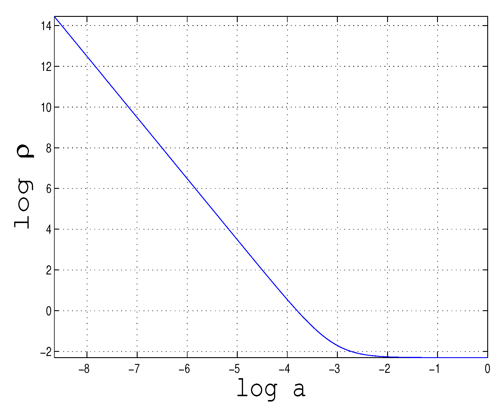
Figure 4.
Evolution of the averaged value that with very high accuracy coincides with the value of in the maximal volume domains of low fermion density. The result of this numerical solution confirms the analytical estimates, the results of which are formulated in the paragraph after Equation (157) under the name of the “self-locking” effect: as the total energy density decays from the value at the cold matter dominated epoch with up to the value at the DE dominated epoch with (see fig.2), changes only from to the fermion vacuum value defined by Equation (149).
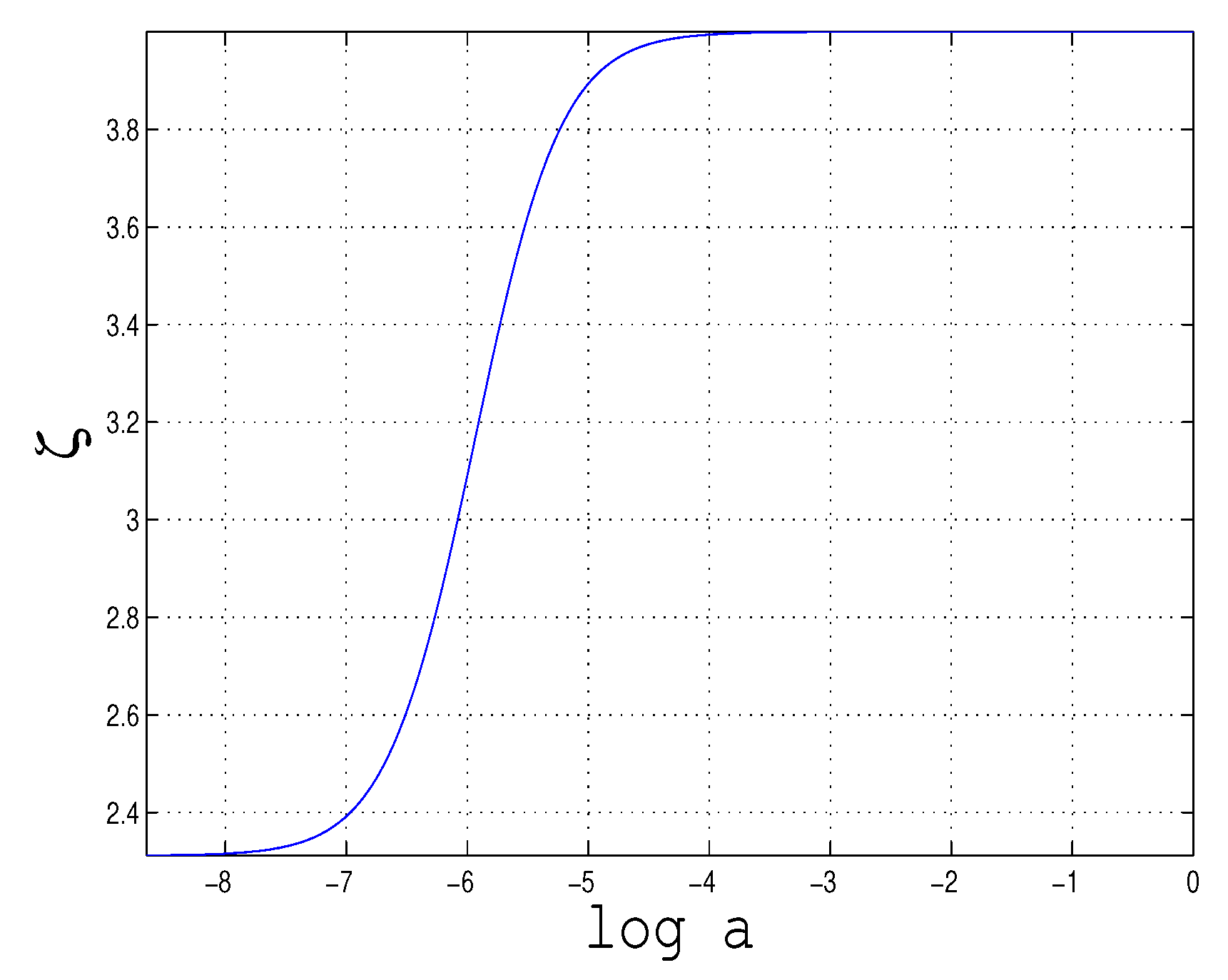
Figure 5.
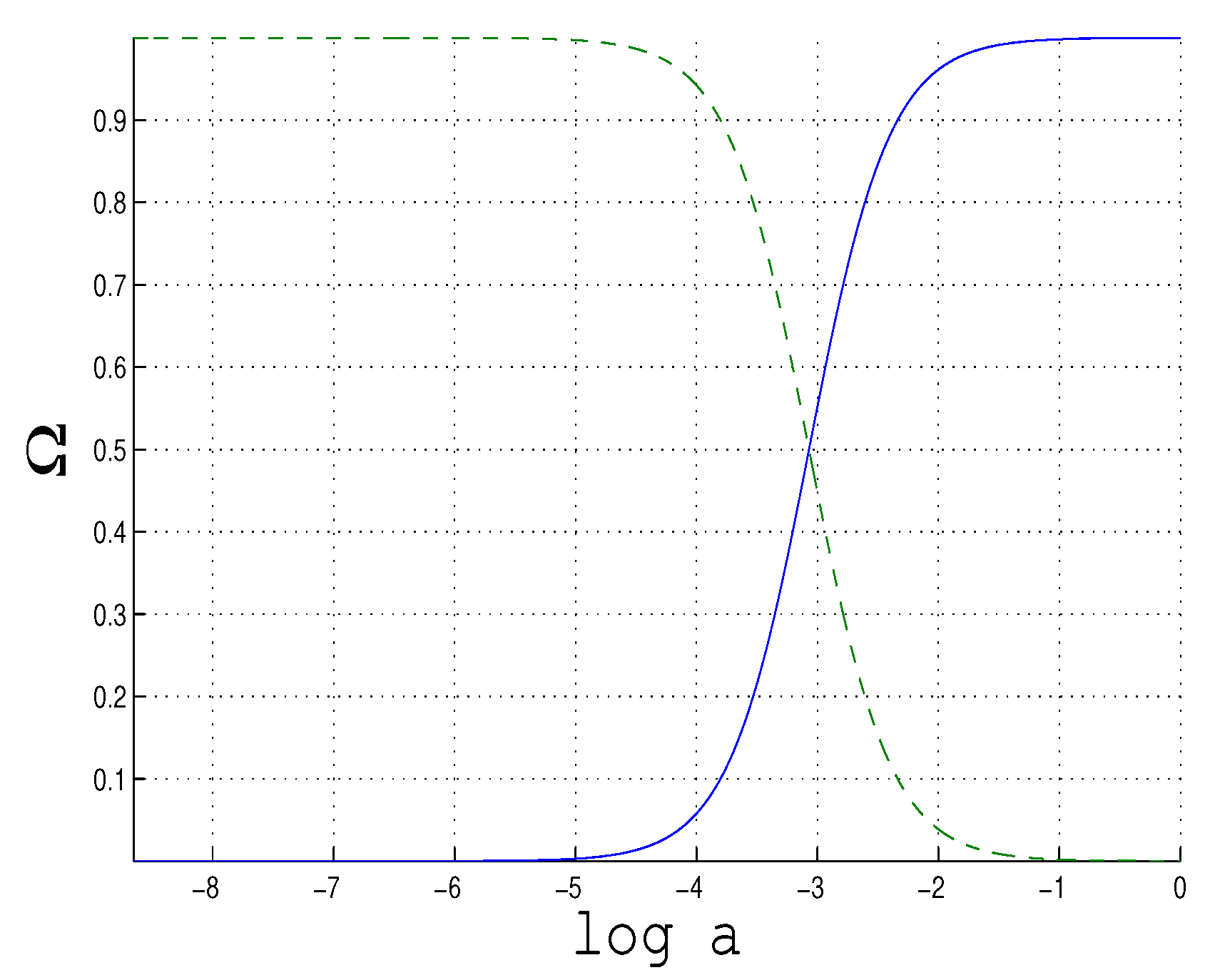
vs where fractions of clustered (dark) matter (the black dash line) and effective DE (the blue solid line).
Figure 5.
vs where fractions of clustered (dark) matter (the black dash line) and effective DE (the blue solid line).
8. A Possible Connection Between the Borde-Guth-Vilenkin Theorem and Initial Conditions for Inflation as a TMT Effect
Conditions that the initial kinetic and gradient energy densities of the canonically normalised scalar field should not exceed the potential energy density
are well known as the constraints neeeded for the onset of inflation. According to the understanding developed in the first models of chaotic inflation [25,26], when the classical space-time domain first appears after the Planck quantum era, the total energy density is of the order of , and inflation begins with . Then all admissible values , , of the classical scalar field satisfying (174 ) can serve as initial values for inflation. At first glance, such an idea of the beginning of inflation cannot contradict the constraintin the last stages of inflation. However, the situation has changed dramatically in light of recent cosmological observations data [10,11] which favor inflationary models with plateau-like potentials, and with the height of the plateau . There exist a number of field theory models in which the plateau-like potentials arise due to the implementation of various original ideas, and these potentials satisfy the CMB constraints. These include the Starobinsky model [27], the Goncharov-Linde model [28], the Higgs inflation models [29]–34]. Of particular interest are -attractor models, which were initiated by the pioneering works [35,36,37] and which have been intensively studied in recent years. To date, there is the broad class of the cosmological attractor models, which generalize most of the previously proposed models with plateau potentials.
Despite such an impressive success of plateau-like models compared to all other models, a lively discussion ensued, during which even the very idea of inflation has been called into question [38]–41]. An obvious disadvantage of the models with plateau potentials mentioned above is the infinite length of the potential energy density plateau. In such a theory, all initial values of the homogeneous component of the scalar field are equally probable. Therefore, an excessively long duration of inflation is possible. The main problem formulated in paper[38] is also related to the height of the plateau , since in this case there is a huge range of possible values of the initial kinetic and gradient energy densities greater than , up to the Planck density. Therefore, in contrast to the understanding developed in first models of chaotic inflation [25,26] of how initial conditions for inflation arise, there is no reason to believe that conditions (174 ) necessary for the onset of inflation are satisfied. A possible response to this challenge may be to modify the model in such a way that the potential has a plateau of finite length, after which, at very large , the potential rapidly increases. An example of this type of model is the "singular -attractor" model proposed by Linde in [42], in which the simplest -attractor potential takes an exponentially steep form for very large . This makes it possible to provide conditions for power-law inflation, which starts at the Planck density, and thus makes it possible to solve the problem of initial conditions in the spirit of [26].
Another, completely independent aspect of the problem of the onset of inflation is predicted by the Borde-Guth-Vilenkin (BGV) theorem. According to the BGV theorem[43] which strengthens earlier proofs of singularity theorems [44,45], in inflationary cosmology almost all past-directed timelike and null geodesics cannot be extended to the past beyond some boundary spacelike hypersurface . The statement of the BGV theorem is quite general because it is based on a kinematic argument. The main problem that inevitably follows from the statement of the BGV theorem is that the inflationary universe must have had some kind of beginning, and, therefore, some new physics is necessary in order to determine the correct conditions at the boundary . However, the BGV theorem says nothing about the boundary conditions on , or even about its location.
This section is based on the TMT-model of paper [46], where it is shown that: (A) there is an exact upper bound of the interval of possible values of the inflaton field in which the onset of inflation is guaranteed; (B) this maximum allowed value determines the location of the boundary spacelike hypersurface that can be identified with the boundary spacelike hypersurface in the BGV theorem. The primordial action is chosen as follows
where
Here and are primordial model parameters, introduced in accordance with the general structure of the TMT primordial Lagrangian density discussed in Section 3. But unlike the models studied in Section 5, Section 6 and Section 7, the action (175) contains, firstly, a -term (39) and, secondly, a non-minimal coupling of the scalar field to curvature with a non-minimal coupling constant .
Following the prescription of the TMT procedure, we must consider the equations of motion that follow from the primordial action (175). Under the condition (5), i.e. everywhere , the consistency of the equations imposes a constraint, and, as usual, a transition to the Einstein frame is necessary. The latter is described by the formula
Then the constraint in the Einstein frame reads as follows
Similar to what was in Section 6.2, the TMT-effective energy-momentum tensor and -equation in the Einstein frame have the structure of the k-essence type model. The minimum of the TMT-effective potential is reached at , and from the constraint (178) it follows that the scalar in this vacuum is equal to
We choose the value of the TMT effective potential in the vacuum, i.e. the TMT-effective CC, to be zero. This can be achieved by choosing the integration constant either or . This is very similar to the toy model from Section 4, and the corresponding values of coincide with and , as in Equations (32) and (33). We choose a solution with and the corresponding , omitting the + sign further. Recall that this also means choosing . To indicate that we are considering a solution with a zero cosmological constant, we will use the symbol in the notation of all relevant quantities. We will also assume that and . After using the redifinition of the scalar field to
which is more appropriate when studying inflation, the constraint (178) reduces to the following
Omitting the explicitly written Einstein equations and the -field equation, in complete analogy with Section 4 and Section 6.2, we use the pressure density, which plays the role of the matter Lagrangian in the TMT-effective action; a variation of the latter yields these equations and is much more convenient to work with. In terms of the field, and after inserting given by the constraint (181), the TMT-effective action takes the form
where the TMT-effective Lagrangian for the scalar field appears as following
where
and for the partameter the parametrization was used. The appearance in the TMT-effective potential the hyperbolic functions like is typical for the simplest T-Model obtained in the conformal theory [35]. An example of the shape of the TMT-effective potential is shown in Figure 6 for the following choice of parameters: , , that is , , , , , . It is similar to a case of the single field attractor models [37], where the hyperbolic functions depend on the combination .
A detailed analysis in [46] shows that in the region of corresponding to the plateau of , the contribution of the last two terms to the TMT-effective Lagrangian (183) is negligible. Consequently, the presence of these terms in (183) does not change the conditions (174) for the onset of inflation. The standard, non-TMT, formulation of the initial conditions for inflation driven by a scalar field includes specifying or at least estimating the initial value of the field and its first derivatives or, equivalently, the initial kinetic energy density and the gradient energy density . It is fundamentally important and taken for granted that there is no dependence in any form between and , as well as between and . But in the studied TMT model the scalar ζ given by the constraint (181) turns out to depend not only on φ, but also on . After choosing the integration constant and, correspondingly, , throughout the entire process of cosmological evolution, must be positive. As a result, the condition imposes restrictions in the form of inequalities on the admissible ranges of and. We are interested in the constraints on the initial values and imposed both by the condition and by the upper bounds on and, Equation (174). Inflation can only begin if all of these conditions are met simultaneously.
The results of the requirement that be positive can be obtained from a detailed study of the inequality
taking into account the significant difference between how kinetic and gradient energy densities enter into the Einstein equations and into the left-hand side of the inequality (189). Indeed, while the kinetic and gradient energy densities enter the Einstein equations in the form of a sum, they enter the constraint in the form
that is, in fact, in the form of a difference. Therefore, can be positive or negative depending on how inhomogeneous and anisotropic at the beginning of inflation was the space domain whose expansion generates our Universe. Since the sign of can significantly affect the results obtained from the condition , the cases and should be considered separately. The main results are summarized below.
Let us start fron considering the constraint (181) at . We see that there exists the value such that when and is defined by the relation
obtained after neglecting a very small correction from the term . In other words, in the case there exists a maximum allowed value such that values are prohibited by the condition , equivalent to , i.e. the infinite interval is an artifact. For the parameters used in the graph in Figure 6, the relation (191) gives . The corresponding point on the curve is marked with a dot.
The analysis of the case in [46] shows that it is impossible to specify precise conditions that guarantee the onset of inflation. It is only worth noting that means the dominance of the spatial gradients of the field , which usually arise due to quantum fluctuations. The interpretation and possible cosmological effect of this result may be of interest, but its study was beyond the scope of the paper [46].
The main results in the case :
1) There exists the minimal initial value defined by the formula
such that on the interval
the condition and the necessary conditions (174) for the beginning of inflation are guaranteed to be fulfilled. For the set of parameters used in Figure 6, we get . With the chosen value of we get that correspoding to 60 e-foldings is , i.e. is inside the interval (193).
Figure 7.
Plot of for the case of the following choice of parameters: , , that is , , , , , . The two dots on the plot correspond to defined by relation (191) and defined by Equation (192).
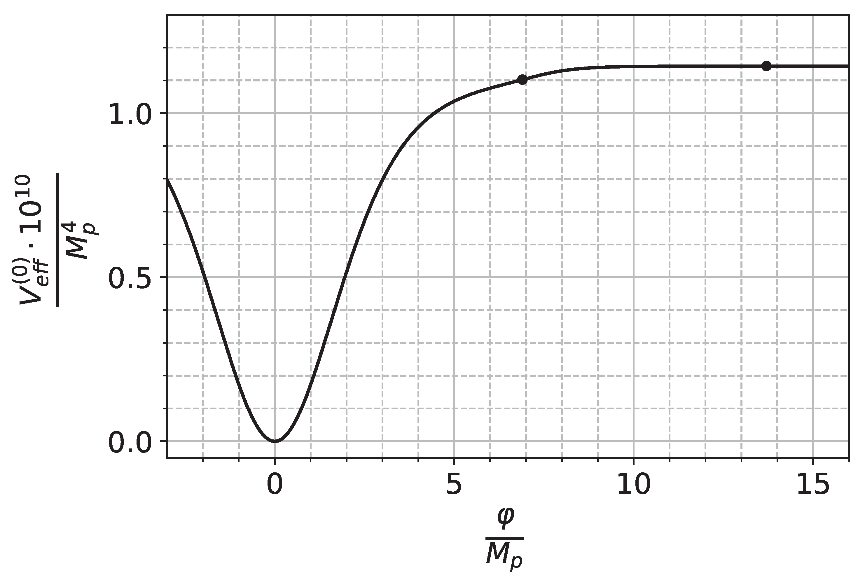
2) It turns out that the upper bound of admissible values of tends to zero as :
Thus, for the case in the plane the point is the boundary point such that cannot be extended to without changing the sign of from positive to negative.
3) In the interval (193) of , the TMT effective potential has a plateau-like shape and is less than the plateau height. Therefore, one can expect that the Universe inflates in the slow-roll regime.
4) For the condition is satisfied, but the conditions (174) required for the onset of inflation may or may not hold.
Initial conditions for inflation and the spacelike character of the hypersurface .
In the model under study (as in all models in the previous sections), we came to the key conclusion: the dynamics of the model dictates that nontrivial solutions exist only when the measure density and, therefore, must be sign-definite. However, the condition (194) can be represented as following
This means that the hypersurface does indeed exist and it separates the space-time manifold into two regions with and , and we must study equations and their solutions in these regions independently of each other. These two regions can be considered as submanifolds of with a common boundary . In what follows we will use the notations and for the submanifolds with and respectively. The condition means that the normal vectors to all hypersurfaces described by the equations are timelike and consequently, the hypersurfaces are spacelike. All of the above remains true for arbitrarily close to . To find out the geometric properties of the hypersurface , we must, given the definition , study what happens to when . In doing this analysis, we must not forget that and are considered independent of each other and serve as initial values for inflation. Therefore, it would be wrong to conclude that because . But we can take into account the very nontrivial result containing in Equation (195): decreases to 0 when . Therefore, for values of very close to the function can be considered approximately as a function depending only on : . Hence, for the equation describes a spacelike hypersurface. The latter remains true when (which is accompanied by ). Therefore,
the hypersurface is a space-like boundary of the submanifold .
It is worth remembering that by applying the principle of least action to the primordial action (175), we mean, as usual, that all primordial variables (scalar field ϕ, non-degenerate metric tensor , the affine connection , the functions and hence Υ) are defined globally on an orientable space-time manifold and are smooth functions. In particular, this means that: 1) they are all continuous on ; 2) one can choose the orientation of . The latter should be expressed in the possibility of choosing a certain sign of . As we have seen, in order to describe our Universe, when solving equations in the model under consideration, we had to put , i.e. choose a positive orientation. Based on our experience in field theory, we might naively expect this condition to still hold globally on . However, it turns out that this is not the case due to the dynamics of the model. The reason for this phenomenon is a very profound change introduced by TMT into field theory: as a result of the inclusion of the variables (from which is built) into the principle of least action, the possibility arises of mutual influence of the matter field dynamics and the continuous function or, in other words, between matter and such a fundamental property of the space-time manifold as orientability. This fundamentally new dynamical effect can lead to the creation of a hypersurface in , which, as we have seen, can in turn impose significant restrictions on the dynamics of mater fields.
The creation of the hypersurface (despite the fact that originally was nonvanishing on ) and the splitting of into two submanifolds and with the opposite orientation means that is not oriented anymore. Since this effect is the result of solving dynamical equations, it can be interpreted as
spontaneous violation of the orientability of
. Moreover, we found that
the dynamically arisen spacelike hypersurface does not allow extension of solutions for from to .
The totality of the obtained results, namely
- impossibility of extension of solutions for from to
- guaranteed onset of inflation subject to (193)
- the spacelike character of the hypersurface and the timelike character of vectors ,
allows us to assume that in the model under study, the spacelike hypersurface is a concrete realization of the spacelike hypersurface from the BGV theorem.
Considering the existence of two submanifolds and with the opposite orientation, the paper [46] also studies question what is hidden behind the space-like hypersurface and boundary conditions on this hypersurface.
9. Discussion
The wide range of applications of TMT to gravity and cosmology is evident from the section headings of the paper. The most important advantage of TMT as an alternative theory is that, under the conditions under which all classical tests of general relativity are performed, TMT accurately reproduces Einstein’s GR. At the same time, TMT offers a number of very interesting models of dark energy. In this paper, we also discussed the new possibilities TMT opens for describing inflation and its initial conditions. In this regard, it is worth noting that refs. [47] and [48], not included in this review, propose a new approach to implementing the Higgs inflation model.
In the final discussion, it makes sense to focus on the fundamentally new ideas underlying TMT and leading to the results presented in the article. First of all, it is necessary to pay attention to the validity of the statement that
the volume elements and are equally natural
. This conclusion, which we reached in the Introduction, Section 1, in the course of our analysis of Wald’s argumentation, is a concept of fundamental importance and there is no longer any reason to continue to ignore the volume measure when constructing field theory models.
In this paper, while demonstrating various TMT models and their highly interesting results, we paid special attention to the effects arising from including the functions, from which Υ is constructed, as degrees of freedom in the primordial action. As we have seen, in all the models studied, these effects are described by a scalar function . Bearing in mind that gravity in GR has a geometric nature described by the metric tensor, we used the term pregeometry for effects caused by the scalar .
One of the pregeometry effects is related to sign-indefinitness of Υ. Therefore, the use of the volume element in the primordial action means that a field theory model is formulated on a space-time manifold orientation of which is initially unfixed. Only after applying the least action principle and choosing a solution to the equations of motion does a specific sign of ζ appear, and hence a specific sign of orientation. Moreover, as we have seen, there always exists another solution corresponding to the opposite orientation sign. Thus, firstly, we are dealing with the pregeometry effect, which consists of
a spontaneous restoration of the space-time orientation
; secondly there is a strict correlation between the physical results predicted by the TMT (via solutions to the equations) and the sign of the orientation of spacetime.
Representing the primordial action as and varying it wih respect to , we find that the solution exists under the condition , that is, only if spacetime is orientable. In this case, only those cosmological solutions (along with their initial conditions and vacuum states) are valid for which does not change sign throughout the evolution of the Universe. This is another pregeometry effect that has played a significant role in all the models considered in this article.
However, when discussing the models under consideration, it is worth noting three special cases where the condition may be violated, which means the orientability of the space-time manifold is lost.
1) In the model of refs.[14] and [15] briefly discussed in Section 6.2, the measure density Υ and the primordial metric oscillate around their zeros during transition to the vacuum state with zero vacuum energy. This means that transition to a state with zero cosmological constant, which occurs in this model without fine tuning, must be accompanied not only by a periodic reversal of the orientation sign but also by passage through a singularity in the primordial metric. Therefore, the assumption of regularity of the function may be violated. This pregeometry effect apparently indicates that attempting to implement TMT models in which zero CC is achieved without fine-tuning requires a more careful analysis of possible solutions in TMT.
2) In ref.[14], studying possible dark energy scenarios for the late time Universe, it was demonstrated that there is a wide range of the primordial model parameters where the superaccelerating cosmological expansion is obtained without introducing an explicit phantom scalar field into the primordial action (59). The numerical solution of the cosmological equations and its detailed analysis in the paper [15] show that during the evolution, the volume measure density Υ changes sign from positive to negative, so that becomes negative. Returning to the primordial action (59), we see that the kinetic term of the ϕ field changes sign, that is, the standard scalar field is dynamically transformed into a phantom field. Some features of this scenario are briefly described in Section 6.2 of this paper, from which it is clear that the sign change of the field ϕ kinetic term in the primordial action (59) occurs simultaneously with crossing of the phantom divide , see Figure 1.
3) An investigation of a possible connection between the BGV theorem and initial conditions for inflation in the paper [46], briefly discussed in Section 8, reveals that the boundary spacelike hypersurface predicted by the BGV theorem does indeed exist, and in the TMT model under consideration this hypersurface is described by the equation . Assuming the continuity of , we showed that, despite the initial assumption , a hypersurface arises, partitioning the spacetime manifold into two submanifolds and with opposite signs of and hence with opposite orientations. Consequently, the equations of motion must be solved separately for and for , where, generally speaking, different integration constants must be chosen. It then turns out that, in the general case, on the hypersurface , there is a discontinuity of the metric tensor used in the Einstein frame.
The author declares no conflicts of interest.
Appendix A. Nonrelativistic Fermions in Section 6.4 and Section 7
In Section 6.4 and Section 7 we study the application of the field theory models to the case of nonrelativistic fermions. This means that we neglect the effect of fermions 3-momenta. The only component of the canonical fermion energy-momentum tensor which survive in this approximation is the energy density . Making use of the Dirac equation in the same approximation we obtain (see also Equations (132) and (142))
To provide the consistent description of the fermion energy density and pressure we have to regard as the field operator. Then the standard semiclassical approach to the Einstein Equations (24) (when the gravity is treated as the classical field) implies the need to evaluate the matrix element of between appropriate states of the Fock space resulting in the fermion (particles and antiparticles) number density n [49]–51]. Then
In the case of nonrelativistic fermions, corrections to the cold fermion approximation reduce to the appearance of the Fermi momentum depending factors in front of n in Equation (A2). For the goals of the present paper it is enough to notice that these factors are positive.
References
- S.W. Hawking, G.F.R. Ellis, The large scale structure of space-time, Cambridge University Press (1973).
- <i>Robert, M. Wald, General Relativity, The University of Chicago Press (1984).
- <i>John, M. Lee, Introduction to Smooth Manifolds, Second Edition, Springer Science+Business Media New York (2013).
- D. Benisty, E. Guendelman, A. Kaganovich, E. Nissimov, S. Pacheva, Modified Gravity Theories Based on the Non-canonical Volume-Form Formalism, Springer Proc.Math.Stat.,335(2019) 239-252 [1905.09933 [gr-qc]].
- E. I. Guendelman and A. B. Kaganovich, Dynamical measure and field theory models free of the cosmological constant problem", Phys. Rev.,D 60(1999) 065004 [arXiv:9905029].
- E.I. Guendelman, "Scale invariance and vacuum energy", Mod. Phys. Lett. A14, (1999) 1043 ; hep-th/0106084.
- E.I. Guendelman, "Scale symmetry spontaneously broken by asymptotic behavior" Class. Quant. Grav. 17, (2000) 361 ; gr-qc/9906025;
- A. B. Kaganovich, "Field theory model giving rise to ’quintessential inflation’ without the cosmological constant and other fine tuning problems", Phys. Rev. D 63 (2001) 025022 [hep-th/0007144].
- P.J.E. Peebles and A. Vilenkin, "Quintessential Inflation", Phys. Rev. D59, 063505 (1999) [astro-ph/9810509].
- Y. Akrami et al. [Planck], Planck 2018 results. X. Constraints on inflation Astron. Astrophys. 641, A10 (2020) [arXiv:1807.06211 [astro-ph.CO]].
- P. A. R. Ade et al. [BICEP and Keck], Improved Constraints on Primordial Gravitational Waves using Planck, WMAP, and BICEP/Keck Observations through the 2018 Observing Season, Phys. Rev. Lett. 127, no.15 (2021) 151301 [arXiv:2110.00483 [astro-ph.CO]]. arXiv:2110.00483.
- E. I. Guendelman, "Scale invariance and vacuum energy", Mod. Phys. Lett. A14, (1999) 1397 ; gr-qc/9901067;
- E. I. Guendelman, "The Volume element of space-time and scale invariance", Found. Phys. 31, (2001) 1019 [hep-th/0011049].
- E. I. Guendelman and A. B. Kaganovich, "Fine tuning free paradigm of Two Measures Theory: K-essence, absence of initial singularity of the curvature and inflation with graceful exit to zero cosmological constant state", Phys. Rev. D 75, (2007) 083505 [arXiv:0607111].
- E. I. Guendelman and A. B. Kaganovich, "Transition to zero cosmological constant and phantom dark energy as solutions involving change of orientation of space-time manifold", Class. Quant. Grav. 25(2008) 235015 [arXiv:0804.1278 [gr-qc]].
- Takeshi Chiba, Takahiro Okabe, Masahide Yamaguchi, "Kinetically driven quintessence", Phys.Rev.D62(2000) 023511 [astro-ph/9912463 [astro-ph]].
- C. Armendariz-Picon, Viatcheslav F. Mukhanov, Paul J. Steinhardt, "Essentials of k essence", Phys.Rev.D63(2001) 103510 [astro-ph/0006373 [astro-ph]].
- J.D. Barrow, "More general sudden singularities, Class.Quant.Grav. 21, L79 (2004); ibid. 21, 5619 (2004) [gr-qc/0409062 [gr-qc]].
- S. Weinberg, "The Cosmological Constant Problem", Rev. Mod. Phys. 61, 1 (1989).
- S. Campo, E. I. Guendelman, A. B. Kaganovich, R. Herrera, Emergent universe from scale invariant Two Measures Theory, Phys. Lett. B 699(2011) 211 [arXiv:1105.0651 [astro-ph.CO]]. arXiv:1105.0651.
- E. I. Guendelman and A. B. Kaganovich, Absence of the fifth force problem in a model with spontaneously broken dilatation symmetry, Annals Phys. 323(2008) 866 [arXiv:0704.1998 [gr-qc]]. arXiv:0704.1998.
- E. I. Guendelman and A. B. Kaganovich, Exotic low density fermion states in the two measures field theory: Neutrino dark energy, Int. J. Mod. Phys A 21 (2006) 4373 [gr-qc/0603070].
- E. I. Guendelman and A. B. Kaganovich, Neutrino generated dynamical dark energy with no dark energy field, Phys. Rev D87(2013) 044021 [arXiv:1208.2132 [gr-qc]]. arXiv:1208.2132.
- N. D. Birrell and P. C. W. Davies, Quantum Fields in Curved Space, Cambridge University Press, 1982.
- A. D. Linde, Chaotic inflation, Phys. Lett.,B 129, 177-181 (1983).
- A. D. Linde, Initial conditions for inflation, Phys. Lett.,B 162, (1985) 281-286 .
- A. A. Starobinsky, A New Type of Isotropic Cosmological Models Without Singularity, Phys. Lett. B 91(1980) 99.
- A. B. Goncharov and A. D. Linde, Chaotic Inflation in Supergravity, Phys. Lett. B 139(1984) 27.
- D. S. Salopek, J. R. Bond and J. M. Bardeen, Designing density fluctuation spectra in inflation, Phys. Rev.D40(1989) 1753.
- F. Bezrukov and M. Shaposhnikov, The Standard Model Higgs boson as the inflaton, Phys.Lett. B659(2008) 703 [arXiv:0710.3755] [inSPIRE]. arXiv:0710.3755].
- Barvinsky, A.O., Kamenshchik, A.Yu. and Starobinsky, A.A., Inflation scenario via the Standard Model Higgs boson and LHC, JCAP 11(2008) [arXiv:0809.2104].
- F.L. Bezrukov, A. Magnin and M. Shaposhnikov, Standard Model Higgs boson mass from inflation,Phys.Lett. B675(2009) 88 [arXiv:0812.4950]. arXiv:0812.4950.
- F. Bezrukov and M. Shaposhnikov, Standard Model Higgs boson mass from inflation: Two loop analysis, JHEP 0907(2009) 089 [arXiv:0904.1537]. arXiv:0904.1537.
- F. Bezrukov, A. Magnin, M. Shaposhnikov, S. Sibiryakov, Higgs inflation: consistency and generalisations, JHEP 01(2011) 016 [arXiv:1008.5157]. arXiv:1008.5157.
- R. Kallosh and A. Linde, Universality Class in Conformal Inflation,” JCAP 1307(2013) 002 [arXiv:1306.5220 [arXiv:hep-th]].
- S. Ferrara, R. Kallosh, A. Linde and M. Porrati, Minimal Supergravity Models of Inflation, Phys. Rev. D 88no. 8 (2013) 085038 [arXiv:1307.7696 [hep-th]]. arXiv:1307.7696.
- R. Kallosh, A. Linde and D. Roest, “Superconformal Inflationary α-Attractors,” JHEP 1311, 198 (2013) [arXiv:1311.0472 [hep-th]]. arXiv:1311.0472.
- A. Ijjas, P. J. Steinhardt, A. Loeb, Inflationary paradigm in trouble after Planck2013, Phys. Lett. B 723(2013) 261-266 [arXiv:1304.2785 [astro-ph.CO]]. arXiv:1304.2785.
- A. H. Guth, D. I. Kaiser, and Y. Nomura, Inflationary paradigm after Planck 2013, Phys. Lett. B 733(2014) 112-119 [arXiv:1312.7619 [astro-ph.CO]]. arXiv:1312.7619.
- A. Linde, Inflationary Cosmology after Planck 2013, Contribution to: Post-Planck Cosmology: Lecture Notes of the Les Houches Summer SchoolVolume 100, July 2013, 231-316 [arXiv:1402.0526 [hep-th]]. arXiv:1402.0526.
- A. Ijjas, P. J. Steinhardt, A. Loeb, Inflationary schism, Phys. Lett. B 736(2014) 142-146 [arXiv:1402.6980 [astro-ph.CO]]. arXiv:1402.6980.
- A. Linde,On the problem of initial conditions for inflation Found.Phys. 48(2018) 10, 1246-1260 (Contribution to: Black Holes, Gravitational Waves and Spacetime Singularities) [arXiv:1710.04278 [hep-th]].
- A. Borde, A. H. Guth, A. Vilenkin, Inflationary space-times are incomplete in past directions, Phys.Rev.Lett.90(2003) 151301 [arXiv:0110012 [gr-qc]].
- A. Borde, A. Vilenkin, Eternal inflation and the initial singularity, Phys.Rev.Lett. 72(1994) 3305-3309 [gr-qc/9312022 [gr-qc]].
- A. Borde, A. Vilenkin, Violations of the weak energy condition in inflating space-times, Phys.Rev. D 56(1997) 717-723 [gr-qc/9702019 [gr-qc]].
- Alexander B. Kaganovich, Possible relationship between initial conditions for inflation and past geodesic incompleteness of the inflationary spacetime, JCAP 05(2023) 007 [arXiv:2209.00378 [hep-th]].
- Alexander B. Kaganovich, Higgs inflation model with small non-minimal coupling constant. arXiv:2501.15597.
- Alexander B. Kaganovich, Two-Measure Electroweak Standard Model. Some aspects of cosmological evolution and vacuum stability. arXiv:2501.15623.
- Rob Fardon, Ann E. Nelson, Neal Weiner, Dark energy from mass varying neutrinos, JCAP 10(2004) 005 [astro-ph/0309800].
- R.D. Peccei, "Neutrino models of dark energy" Phys. Rev. D71 (2005) 023527 [hep-ph/0411137].
- T. Goldman, G.J. Stephenson, Jr., P.M. Alsing, B.H.J. McKellar, "A Possible Connection Between Massive Fermions and Dark Energy" Contribution to: DARK 2009, 180-193 [0905.4308 [hep-ph]].
Figure 1.
For the model with , , and and with the the initial conditions , : crossing the phantom divide and changing sign of the total volume measure in the scalar field kinetic term (in the primordial action (59)) occur simultaneously. The figure is copied from ref.[15], where was used instead of .
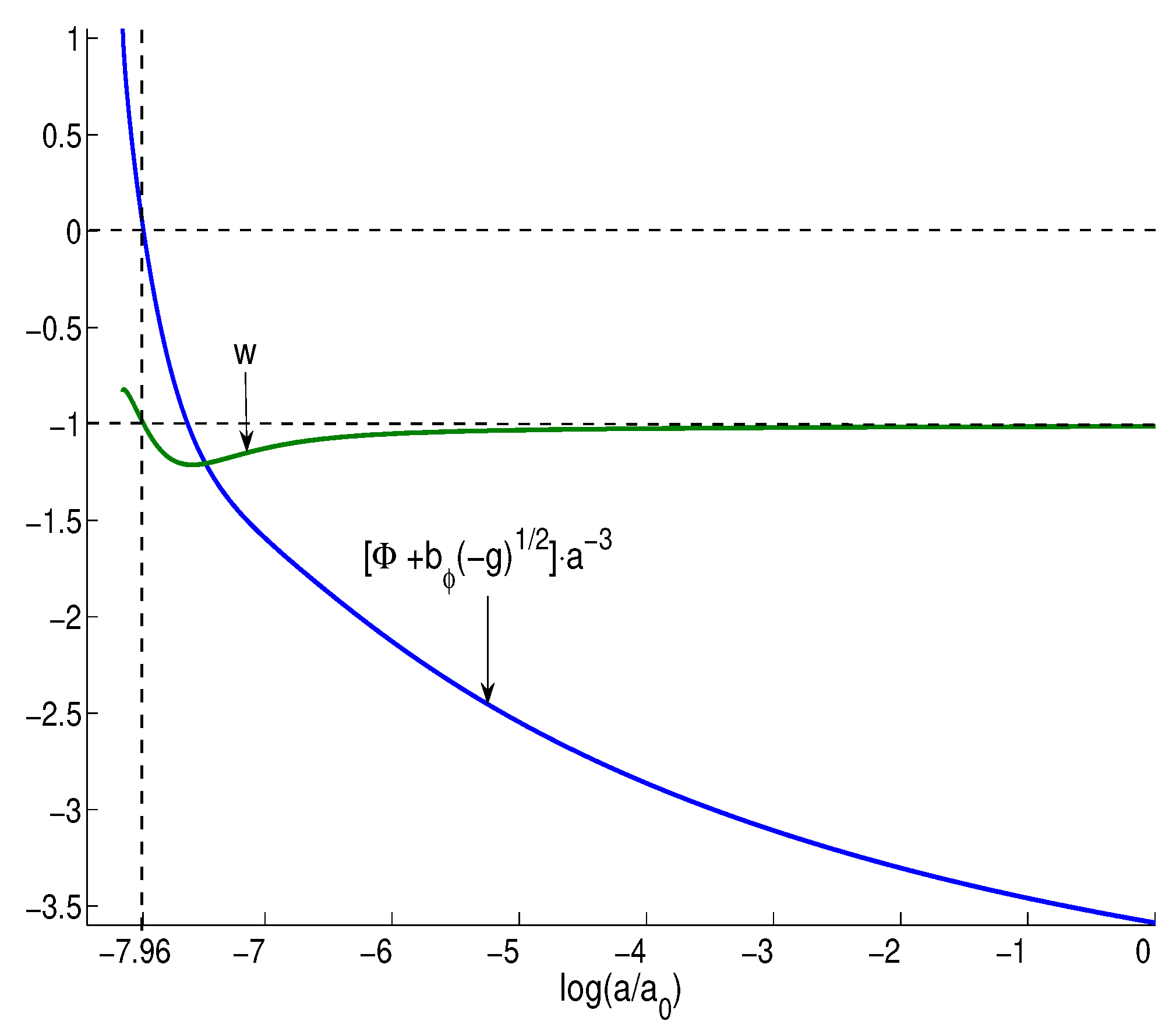
Figure 2.
Total EoS vs .
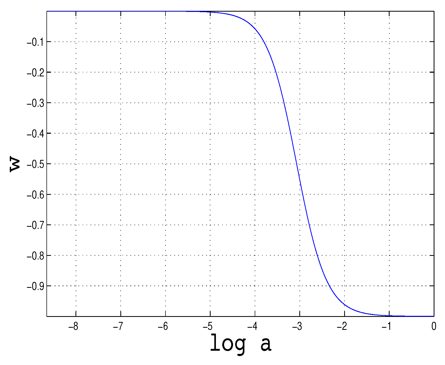
Figure 6.
Mass of the cold neutrinos in the maximal volume domains of low density: m vs and m vs .
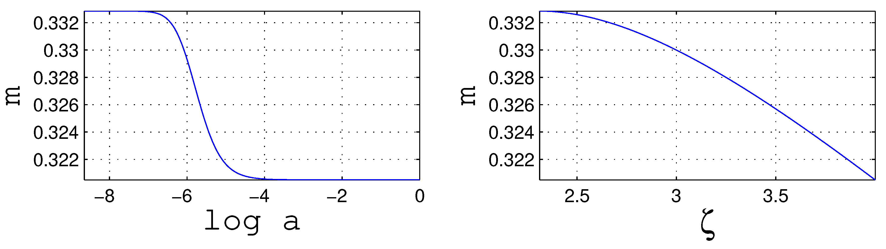
Disclaimer/Publisher’s Note: The statements, opinions and data contained in all publications are solely those of the individual author(s) and contributor(s) and not of MDPI and/or the editor(s). MDPI and/or the editor(s) disclaim responsibility for any injury to people or property resulting from any ideas, methods, instructions or products referred to in the content. |
© 2025 by the authors. Licensee MDPI, Basel, Switzerland. This article is an open access article distributed under the terms and conditions of the Creative Commons Attribution (CC BY) license (http://creativecommons.org/licenses/by/4.0/).
Copyright: This open access article is published under a Creative Commons CC BY 4.0 license, which permit the free download, distribution, and reuse, provided that the author and preprint are cited in any reuse.


