Submitted:
11 October 2025
Posted:
14 October 2025
You are already at the latest version
Abstract
The current research paper investigates the logistic q−distribution q−L(0, 1) from a pro-
babilistic perspective. Its unique characteristics lie in its probability density function (pdf),
cumulative distribution function (cdf), mean, and variance. We introduce the q−Fourier
transform and a new q−differential equation within the framework of quantum calculus and
provide its solution in order to facilitate the characterization of the logistic q−distribution.
A characterization of the relationship between the logistic q−distribution and exponential
q−distributions is determined via the cumulative distribution function (cdf).
Keywords:
q-calculus
; logistic q-distribution
; q-Fourier transform
; q-differential equation
; exponential q-distributions
1. Introduction
Quantum calculus, which stands for a contemporary field of study, addresses the principles of calculus without the traditional reliance on limits. Over the recent years, several research works have been oriented towards q-calculus [1,2,3,4,5], a branch of mathematics that bridges the gap between mathematical theory and physical applications. The origins of quantum calculus date back to the pioneering work of F.H. Jackson [5] in the early 20Th century. A comprehensive overview of the fundamental concepts of quantum calculus is displayed in the book written by Kac and Cheung [11]. Chung et al. [13] introduced the q-addition operator and explored its properties, subsequently applying it to the study of the q-logarithmic and q-exponential functions [17]. The applications of quantum calculus extend to a wide range of mathematical domains, including number theory, difference equations (as exemplified in [6]), orthogonal polynomials, and probability theory.
Within the framework mathematical physics and probability, the q-distribution transcends classical distributions in terms of generality. Diaz [15] introduced this concept in the continuous domain, while Charalambos [3] extended it to the discrete domain. The q-distribution entails constructing a q-analogue of the conventional distribution. Mathai [8] examined the q-analogue of the gamma distribution as far as Lebesgue measure is concerned.
The central target of this paper is to establish a quantum representation for the standard logistic distribution within the framework of quantum calculus logistic q–distribution noted by q–L. This representation is particularly designed for the interval , the q–analogue of , where 0 denotes the location parameter and 1 designates the scale parameter.
At this level, the value of is determined by the formula , with q being a fixed number falling within the range of 0 to 1 and being the q–analogue of in quantum calculus.
As q approaches 1, the representation converges back to the ordinary logistic distribution.
To achieve the quantum representation of the logistic distribution, we need to find the q-analogues of key elements: , , and 1.
Jackson in [5,6] set forward the q-analogue of the exponential function determined by
and
It is clear that , implying that it is based on the convention and
Then, the q-analogue of the function is determined by function , while the Lebesgue measure is replaced with the Jackson measure . To represent 1 in the quantum context, we introduce a new function named . By accomplishing these steps, we establish the desired quantum representation of the Logistic distribution, offering deeper insights into the interplay between quantum calculus and traditional ones.
The q–analogue of the Riemann integral in quantum calculus is provided by the Jackson integral, also known as q–integral. Using the q–integral and the q–analog of the classical exponential function, denoted by , we can introduce a new definition of the Fourier transform in quantum calculus, called the q–Fourier transform. At this stage, q is a real number lying strictly between 0 and .
The q–Fourier transform plays a crucial role in characterizing the logistic q–distribution, denoted by . Furthermore, we can invest solutions in q–differential equations to further demonstrate the characterization of this distribution.
In , the density of the exponential q–distribution is indicated by
and the q–cumulative function of the exponential q–distribution is expressed as
We recall certain basic definitions recorded in [5,6,8,12]. We fix a real number 0 < q < 1. We shall start with the q–derivative and the Jackson q–integral. The q–derivative of function at is determined in terms of
It is also known as the Jackson derivative. We notice that it is linear. In this respect,
It has a product rule analogous to the ordinary ones, with two equivalent forms:
Similarly, it satisfies a quotient rule,
For example the q–derive of function for an integer is indicated by:
where
A right inverse of the q–derivative is obtained via the Jackson integral. For the Jackson integral or q–integral of the function on is expressed as:
It is clear that if q approaches 1, the q–derivative approaches the Newton derivative and the Jackson integral approaches the Riemann integral.
The q-analogue of the rule of integration by parts is provided in terms of:
2. Logistic q-Distribution
The basic purpose of this paragraph is to introduce the modeling of the probability density function of the logistic distribution within the framework of quantum calculus. The function representing this density is denoted as and is defined on the interval , where is a specific parameter associated with the distribution.
We also know that
therefore
If x goes to 1, then we obtain
Hence,
From this perspective, we define the normalizing constant by
Proposition 1.
The normalization constant tends to 1 as q approaches 1 with .
Démonstration.
Since
then
Thus,
□
Figure 1 depicts a plot of as a function of q.
Figure 1.
Plot of as a function of q.
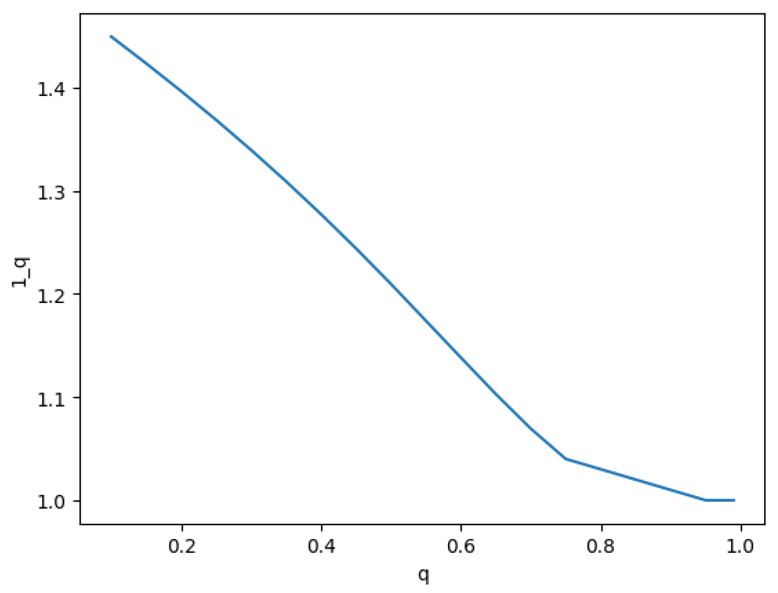
Note that c(q) approaches 1 as q goes to 1.
We are now prepared to formally introduce the logistic q–distribution.
Definition 1.
The probability q-density function of the standard logistic q-distribution, denoted by , is specified by
and for the normalizing constant.
Remark 1.
3. Logistic q–Cumulative
The q-cumulative q-distribution function(q-cdf), of a real random variable X follows q-density , which is provided , for , .
Theorem 1.
The standard logistic q-distribution has a q-cumulative q-distribution function defined as follows
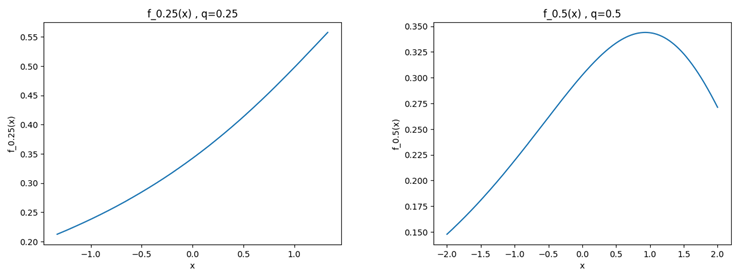
Figure 2 exhibits the logistic q–density curves, for different values of q. It is worth noting that as q tends to 1, the logistic q–density become compatible with the ordinary case.
Démonstration.
For , using the definition 2.1, we get
□
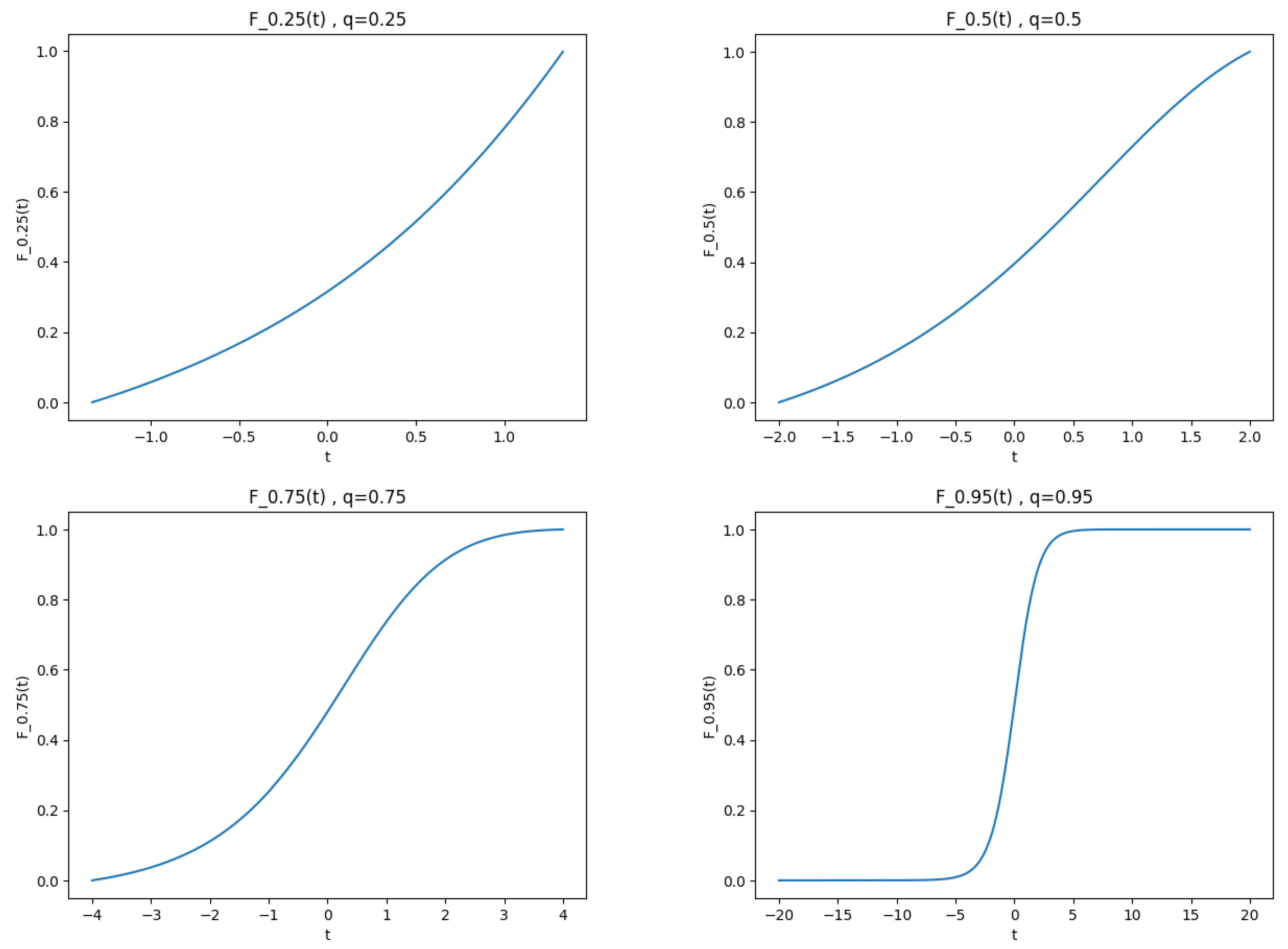
Figure 3 plots the curves of the logistic q-cumulative q-distribution function for different values of q. We notice that this function is always monotone. Besides, the curve converges to the logistic cumulative distribution function curve when q tends to 1.
Remark 2.
We have:
- 1.
- 2.
4. q-Expected and q-Variance Values
In quantum calculus, the q–expected and q–variance of standard logistic q–distribution are well defined with q–expected and q–variance representing the q–analogue of ordinary expected and variance.
Díaz et al. [15,16] introduced the notion of moment in the theory of the q–calculus. It is expressed as follows:
The q–mean of a random variable X with q–density function is expressed by
The q–variance of a random variable X with q–density function is indicated by:
Theorem 2.
Let X be a random variable with a q-density of the standard logistic q–distribution. Then,
- 1.
- The q-expected of X is provided by
- 2.
- The q-variance of X is denoted by
- Let is q-density of standard logistic q–distribution. In this regard, for
-
We have,As a result,
5. q–Fourier Transform
In this section, we use the q- exponential and the definition of the Jackson q-integral as well as its properties to define the q-Fourier transform and determine certain properties that characterize this operator.
The q-exponential is bounded for all x in , where i denotes the imaginary unit.
The q–Fourier transform can be used in the analysis and the resolution of problems in quantum calculus.
With q always being a fixed number falling within the range of 0 to 1.
Definition 2.
The q–Fourier transform of a function f, denoted by , is a function defined on by:
Remark 3.
Let . Then, the q-derivative of q–exponential is written as
Proposition 2.
Let f be a function and its q–derivative. Accordingly, if f and are q–integrable on , then the q–Fourier transform of in is determined by the following relation:
- 1.
- 2.
The q–Fourier transform of f is provided by
Therefore,
- 1.
-
Using the q–integration by parts, we obtain:According to the definition of the q–Fourier transform, we can infer that:Consequently,Thus,
- 2.
-
Since , then and since , then .The q-Fourier transform of the function is expressed in terms ofUsing the q–integration by parts, we obtainAccording to the definition of the q–Fourier transform, it follows thatTherefore,Hence,
Proposition 3.
The q–Fourier transform has the following properties:
- 1.
- Linearity: Let f and g be two functions such that their q–Fourier transforms are indicated respectively by and . Then,
- 2.
- If f is an even function, then the q–Fourier transforms is denoted by
- 3.
- If f is an odd function, then the q–Fourier transforms is stated as
- 4.
- Let , where is a bounded function, then the q-derivative of the q–Fourier transform is specified by
- 1.
- Let be two functions. For all , we get
- 2.
-
The function is an even function and the is an odd function. From this perspective,Therefore,Since f is an even function, we have
- 3.
- Since f is an odd function, we have
- 4.
- The q-derivative of the q–Fourier transform is obtained by:
6. A Characterization of the q–Logistic q-Distribution
The new characterization of the standard logistic q–distribution q–L rests upon a novel procedure, namely the q–Fourier transform and the q-Differential Equation.
A characterization of the relationship between the logistic q–distribution and the q–exponential distributions is determined via the cumulative distribution function (cdf).
6.1. q-Differential Equations
Let g be a q–differentiable function. We define the q–differential equation as follows:
The solutions of are represented by the following proposition:
Proposition 4.
The q–differential equation admits the solution:
We set Then,
Accordingly,
6.2. A Characterization
The following proposition presenting a crucial equivalence is identified to determine the new characterization of law Logistic q-distribution.
Proposition 5.
Let f be a positive continuous function. Hence,
if and only if
We suppose that is a q–primitive of f. Therefore,
It follows that for all
This results in the function which is constant for all
Thus,
Theorem 3.
Let X be a random variable that has an absolutely continuous q-density function, denoted by , and a q-expectation, denoted by . The random variable X adheres to the standard logistic q-distribution, denoted by , if and only if:
holds for all , where
and i denotes the imaginary unit, f q–density.
Suppose X follows the logistic q–distribution q–L. Thus:
Consequently,
is equal to
From this perspective,
It therefore follows that
Let X be a random variable with an absolutely continuous q–density function such that:
and
Using the q–Fourier transform, we infer that:
We get,
Since , relying upon proposition , we get
Based on properties of the q–Fourier transform, we hence note that must satisfy the q–differential equation which is indicated by:
and
With reference to proposition , the solutions of the q–differential equation are determined by:
Since , then
The sole solution of that satisfies
is determined to by
Thus,
and is the q–density of logistic q–distribution q–L.
We prove the following theorems, which establish a new characterization between the logistic q-distribution and the exponential q-distribution with parameter 1.
Theorem 4.
Let X be a continuous q–distributed random variable with a probability q–density function . Then, the random variable is a q–logistic random variable if and only if X follows an exponential q–distribution with parameter 1 in the interval .
The probability q–density function of an exponential random variable X with parameter 1 is identified as follows [9]:
Since , then and
Suppose that the random variable Y follows the logistic q–distribution q–L. Then,
We have
The corresponding result represents the q-cumulative q-distribution function of the exponential q-distribution with parameter 1.
Then, X follows the exponential q–distribution.
Conversely, suppose that the random variable X follows the exponential q–distribution with parameter
We have,
The obtained result represents the q-cumulative q-distribution function of the logistic q–distribution.
Accordingly, Y follows the logistic q–distribution q–L.
Conclusion
In the current investigation, we introduced the logistic q-distribution q–L and characterized the logistic q-distribution q–L, utilizing the q-Expected, the q-Fourier transform and the solution of the q-Differential equation. We equally proved the relationship between the logistic q-distribution and the exponential q-distributions.
The goodness of fit of our findings was ensured via enacting a comparison with the logistic distribution. As q approaches 1, the logistic q-distribution converges to the standard logistic distribution. These results establish significant connections among continuous q distributions and stand for an outstanding step in the area of data processing and simulation studies.
References
- Boris. A. Kupershmidt, q-Probability: I. Basic discrete distributions, J. Nonlinear Math. Phys. 7 (1) (2000), 73-93. [CrossRef]
- Bai, Y., Papageorgiou, N.S. Zeng, S. Anisotropic (p, q)-equations with superlinear reaction. Ricerche mat (2022). [CrossRef]
- C.A. Charalambides, Discrete q-distributions. Wiley, Hoboken. (2016) 1-264.
- D. V. Lindley, Fiducial distributions and bayes’ theorem. J.R. Stat. Soc. Series B (Methodological), ( 1958 ) 102-107. [CrossRef]
- F.H. Jackson, On a q-definite integrals, Q. J. Pure Appl. Math. 41(15) (1910), 193-203.
- F.H. Jackson, On a q-functions and a certain difference operator, Trans. R. Soc. Edinb. 46 (1908), 253-281. [CrossRef]
- Imed, B., Mouna, Z. Estimation Parameters for the Continuous q-Distributions. Sankhya A (2022). [CrossRef]
- I. Boutouria, I. Bouzida and A. Masmoudi, On Characterizing the Gamma and the Beta q-distributions, Bull. Korean Math. Soc. 55(5) (2018), 1563–1575. [CrossRef]
- I. Boutouria, I.Bouzida and A. Masmoudi, On Characterizing the Exponential q-Distribution, Bull. Malays. Math. Sci. Soc. 42 (2018), 3303–3322. [CrossRef]
- I. Bouzida, A. Masmoudi and M. Zitouni, Estimation parameters for the Binomial q-distribution, Commun. Stat. - Theory Methods.0 (0) (2020), 1-13. [CrossRef]
- K. Kac and P. Cheung, Quantum Calculus, Springer-Verlag, Berlin, (2002).
- Kara, H., Budak, H. On Hermite–Hadamard type inequalities for newly defined generalized quantum integrals. Ricerche mat (2021). [CrossRef]
- M. Zitouni, M. Zribi and A. Masmoudi, Asymptotic Properties of the Estimator for a Finite Mixture of Exponential Dispersion Models, J. Filomat. 32(19) (2018), 6575–6598. [CrossRef]
- M. Zitouni, The Kumaraswamy-Rani Distribution and its Applications, J. Biometrics and Biostatistics. 11(1) (2020), 1–4.
- R.Díaz and E.Pariguan, On the Gaussian q-distribution, J. Math. Anal. Appl. 358 (2009), 1-9. [CrossRef]
- Díaz R., Ortiz C., Pariguan E., On the k-gamma q-distribution, J. Math. cent. Eur., 2010, 8(3), 448-458. Ernst T, The History of q-Calculus and a New Method, U. U. D. M. Report 2000:16. [CrossRef]
- Ernst T, The History of q-Calculus and a New Method, U. U. D. M. Report 2000:16, ISSN 1101-3591, Department of Mathematics, Uppsala University, 2000.
Figure 2.
q–Logistic q-density.
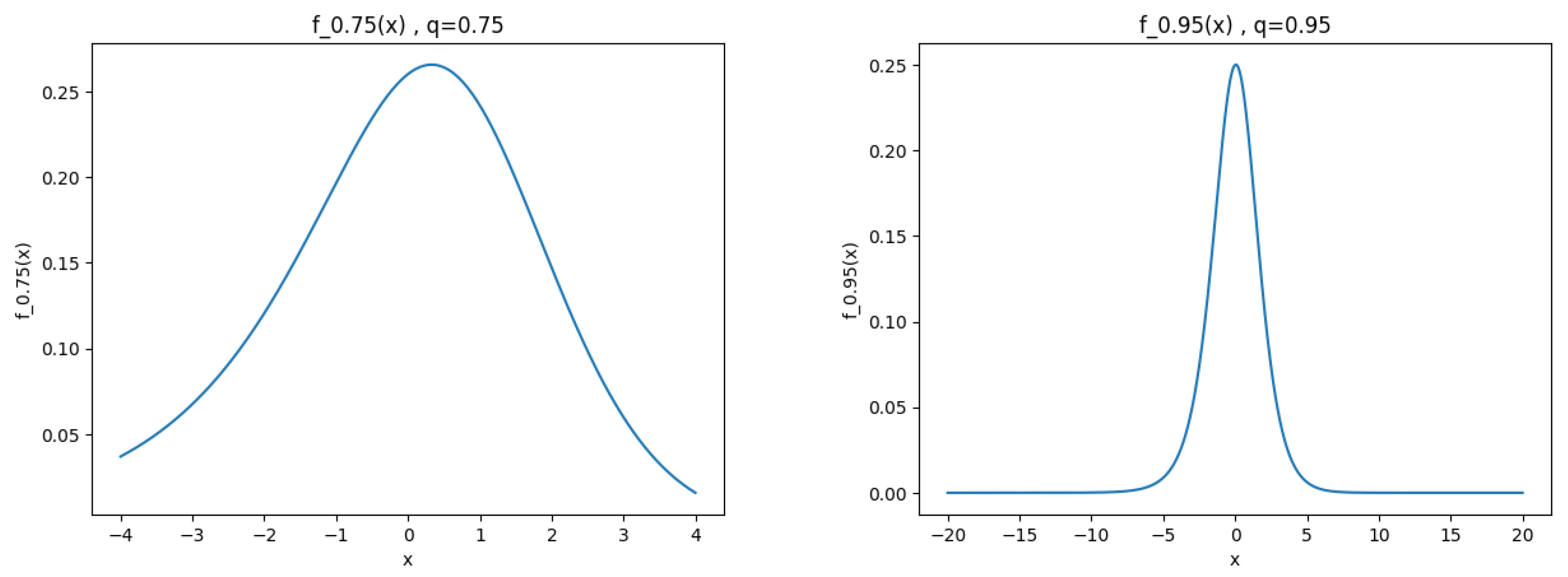
Figure 3.
Logistic q-cumulative.
Disclaimer/Publisher’s Note: The statements, opinions and data contained in all publications are solely those of the individual author(s) and contributor(s) and not of MDPI and/or the editor(s). MDPI and/or the editor(s) disclaim responsibility for any injury to people or property resulting from any ideas, methods, instructions or products referred to in the content. |
© 2025 by the authors. Licensee MDPI, Basel, Switzerland. This article is an open access article distributed under the terms and conditions of the Creative Commons Attribution (CC BY) license (http://creativecommons.org/licenses/by/4.0/).
Copyright: This open access article is published under a Creative Commons CC BY 4.0 license, which permit the free download, distribution, and reuse, provided that the author and preprint are cited in any reuse.


