
Submitted:
13 October 2025
Posted:
14 October 2025
You are already at the latest version
Abstract
Simulating wave propagation is crucial for forecasting processes offshore and near the coast. Many operational wave models consider only atmospheric and wave forcing as boundary conditions. However, waves and currents are interdependent and simulating their interaction is crucial for accurately representing wave propagation. This study examines the influence of current velocity and water levels on waves in the southern coast of the Iberian Peninsula. These forcing elements were simulated by a 3D hydrodynamic model MOHID and included in the Simulating WAves Nearshore (SWAN) model. The standalone SWAN model was calibrated and validated by comparing results of significant wave height, mean wave direction, and peak period with in-situ observations. Then, the effects of water levels and current velocities on wave propagation were assessed by forcing the SWAN model with water levels as well as current velocities extracted from different depths: the surface layer and depth-averaged velocities from the surface down to 10 m, 20 m, and the full water column. The results revealed that incorporating current velocity and water levels from MOHID in the SWAN model reduced RMSE between 1.6% and 27.6%. The most accurate results were achieved with model runs that included both current velocity from the surface layer and water levels. Opposing currents resulted in increases in wave height whereas following currents resulted in decreases in wave height. This work presents novel results on the effects of hydrodynamics on wave propagation along the southern coast of the Iberian Peninsula, a region of key importance for the blue economy.
Keywords:
Wave modeling
; wave-current interaction
; SWAN
; MOHID
; SW Iberia
1. Introduction
The simulation of wave propagation is strongly determined by a variety of forcing conditions including wind, wave, bottom friction, bathymetry, sea surface height, and current velocity. Numerical models are powerful tools that can simulate and predict the interactions between these factors dynamically at fine spatial scales and accurately portray wave propagation. This is crucial for coastal engineering, forecasting storm events, analyzing sediment transport, and gaining a deeper understanding of shallow water processes. For forecasting purposes, besides the lateral boundary conditions, many operational wave models include only atmospheric input in their predictions of wave propagation, as modeling both hydrodynamics and wave propagation can be computationally expensive [1,2]. However, the integration of wave and hydrodynamic models has been shown to improve model performance by reducing the bias and error of simulated wave results [3,4]. Consequently, the study of wave-current interaction has been of recent interest and many wave models are commencing now to incorporate hydrodynamic forcing such as current velocity and water levels.
The interaction between waves and currents is complex as the wave spectrum consists of various components that respond differently to currents and thus there is no simple relationship between these two processes [5]. Currents are influenced by multiple variables, including wind stress, tides, and density gradients. At the same time, wind stress can be affected by the sea state, as surface waves modify air-sea momentum transfer [6,7]. The sea state, in turn, depends on wind stress and currents, creating complex feedback mechanisms between waves and hydrodynamics [7]. The interaction between hydrodynamic and wave models can allow for the exchange of information between these complex processes and can improve our understanding of the non-linear interactions between them. More explicitly, the integration between wave and hydrodynamic models allows for the computation of wave-current interaction processes, which include wave radiation stress and enhanced orbital velocities, which further influence water circulation and sediment transport [8]. Hydrodynamics directly impact the wave field by causing the Doppler effect to occur as well as refraction induced by currents [6]. This amount of refraction depends on the current velocity, the incident wave direction compared to the current, and the wave period [9]. On one hand, the Doppler effect can be seen when waves travel with a current (following current), and the observed frequency decreases. On the other hand, when a wave meets a current from the opposite direction (opposing current), the observed frequency increases and the waves appear to be moving faster [10,11]. Longuet-Higgins and Stewart [10] were some of the first researchers to discover changes in wave amplitude due to the non-linear interactions between waves and currents. More recently, several studies have found that an opposing current directly impacts the wave by increasing the wave height, while a following current increases the mean wavelength, which in turn leads to a decrease in wave height [9,12,13]. This change in the spatial distribution of the wave action has been observed by Barnes and Rautenbach [9] who used SWAN to assess the influence of currents in the strong Agulhas Current System off the coast of South Africa. These authors found increases in significant wave height of 20 – 40% with an opposing current and decreases of approximately 20% in the case of a following current. Similarly, Saruwatari et al. [14] observed changes in wave energy of up to ± 60% when implementing SWAN around the Orkney Islands in Scotland where tidal currents exceed 3 m/s. In a weaker current system off the south coast of Ireland, Calvino et al. [2] also found redistribution of the wave action when implementing WAVEWATCH III forced with surface currents. These authors stated that these significant changes in the wave field would not have been captured without hydrodynamic forcing, highlighting the need to include these parameters in wave models for an accurate representation of the wave field.
Several studies have found improvements in wave model results when adding current velocity as a forcing condition of the wave model [2,5,6,9,13]. The magnitude of improvement showed to be dependent on how accurate the modeled current fields are as well as the location of the wave/current regime. For example, Barnes and Rautenbach [9] found only minor improvements of 0.01 to 0.02 m in significant wave height accuracy when forcing their SWAN wave model with a surface current field obtained from the Operational Mercator global ocean model. In another study in the North Atlantic Ocean off the coast of Ireland, the highest change in significant wave height was approximately 10 cm when comparing results from a WAVEWATCH III simulation forced with surface currents and the same simulation without current velocity forcing [2]. Marechal and Ardhuin [5] found that forcing their WAVEWATCH III model with a well-resolved surface current field could accurately capture significant wave height gradients in the Agulhas Current System when comparing their results with satellite altimetry data. In a fully integrated wave-hydrodynamic model (NEMO and WAVEWATCH III) for the Black Sea, Causio et al. [6] found improvements in both the wave field and hydrodynamics when they considered the wave-current interaction in their model. A fully two-way coupled model between an unstructured 2D ocean circulation model Advanced CIRCulation (ADCIRC) and SWAN used depth-averaged currents for the 2D current field and was able to accurately simulate wave propagation in deep and shallow waters in the Gulf of Mexico and Louisiana during four hurricanes [15].
The majority of previous numerical studies have considered only surface currents or the full depth-averaged current velocity field, but none of these aforementioned studies have deeply investigated the depth at which current velocity impacts the wave field. This is especially true for the south coast of Portugal where very few modeled studies on the wave regime exist. Silva et al. [16] implemented the WAVEWATCH III and SWAN models to simulate waves off the Iberian Peninsula and further assess the spatial distribution of wave energy. These authors used the default SWAN settings to run a three-year hindcast and did not consider the effects of currents in their wave model [16]. Rusu et al. [17] also developed a wave forecasting system based on SWAN for western Iberia, but did not force their model with currents. In a nearshore wave-hydrodynamic study in the western margin of the south coast of Portugal, Horta et al. [18] implemented the Steady State Spectral WAVE (STWAVE) model along with field observations to understand how the orientation of the coast impacts nearshore water circulation in different wave conditions. These authors found that the angle at which the waves approach the coastline strongly determines whether the water circulation will be dominated by longshore currents or rip currents [18]. While this study highlights the significance of the effects of waves on water circulation at a specific site along the south coast, the effects of currents on wave propagation along the entire coast have yet to be investigated. To our knowledge, this is the first comprehensive study quantifying the effects of currents and water levels on wave propagation modeling in this region. The spatial variability of the effects of currents associated with the different circulation patterns in the region are also analyzed. Furthermore, the experiments implementing different hydrodynamic forcing in the wave model can be generalized to other regions. This study consists of novel results on how current velocity and water levels impact wave propagation in the south coast of Portugal and sets the stage for future work on how wave propagation influences water circulation by coupling both processes in a fully operational modeling system.
2. Materials and Methods
2.1. Study Area
The study area covers the southern coast of the Iberian Peninsula (southwestern Europe), located in the North Atlantic Ocean (Figure 1). Ocean circulation patterns in this region are complex as the Azores Current separates the oceanic gyre circulation into the Portugal Current in the north and the Canary Current in the south [19]. Furthermore, the entrance to the Mediterranean Sea allows the exchange between two different water masses, which further impacts the regional circulation [20]. The Portugal Current flows southward year-round along the west coast of Iberia [21]. In summer, predominantly northeasterly winds transport water southward along the west coast of Portugal. In autumn and winter the wind direction shifts to southwesterly, reversing the surface circulation and forming the Portugal Coastal Counter Current that flows northward for all layers in the water column from the surface to a depth of ~1500 m [19]. Mesoscale activity is the dominant factor influencing the meteo-oceanographic variability in the region, with variations in coastal alongshore wind stress occurring on a timescale of several tens of days [22].
The region is furthermore part of the Canary Current Upwelling System (CCUS), which extends from 43°N to 10°N along the west coast of Iberia to the northwest coast of Africa. Upwelling off the west coast of Portugal occurs in spring and summer when surface water along the coastline is transported offshore due to the combined effects of the northeasterly winds and the Coriolis force. [21]. Off the southern coast of Portugal, the Portugal Coastal Countercurrent transports warm surface water westward in winter [23]. Once these waters reach the furthest western point along the south coast of Portugal at Cape São Vicente, they occasionally rotate clockwise and are further transported northward along the west coast [23]. The northward transportation of surface water along the west coast produces downwelling events [22].
The wave regime in the region is characterized by dominant more energetic waves coming from W-SW and less energetic E-SE waves [24]. In the south coast of the Algarve the average significant wave height offshore is 0.9 m. Storm wave events are marked by waves reaching a significant wave height of more than 3 m and an associated peak period of 10 – 12 s [25]. Storms occur typically with waves coming from W-SW or E-SE, the former being more frequent and energetic [24]. Waves are much more energetic off the west coast, with average significant wave heights ranging between 2 and 3 m and peak periods between 9 and 11 seconds [26].
The coastline along the south coast of Portugal is highly variable as Cape Santa Maria at 36.97°N, 7.90°W splits the south coast into western and eastern margins. The western margin extends from Cape São Vicente to Cape Santa Maria and the eastern margin extends from Cape Santa Maria to the Guadiana River at the border between Portugal and Spain [27] (Figure 1). The western margin consists of a cliff-dominated, rocky coastline with pocket beaches and is fully exposed to W-SW wave conditions [18]. The eastern margin consists of mainly sandy beaches in front of the Ria Formosa barrier system and lagoon and is fully exposed to E-SE waves [27].
2.2. SWAN
The Simulating WAves Nearshore (SWAN) model, developed at Delft University of Technology, is a third-generation wave model that simulates waves in coastal and inland waters. SWAN solves the full spectral balance equation, incorporating source and sink terms. Since SWAN is a third-generation model, the wave spectrum can propagate freely without any constraints on its evolution. All processes of wave generation, dissipation, and wave-wave interaction are represented [28]. The spectral balance equation is shown below [28].
The terms on the left describe: 1) the action density rate of change ) at a single point in space over time , which is further equivalent to E/ where E is the energy density and is the relative frequency, 2) propagation of wave energy in two-dimensional geographical -space where is the group velocity and is the ambient current velocity vector, 3) shifts in frequency due to currents and changes in depth, and 4) depth- and current-induced refraction. The term on the right represents the sources and sinks of wave energy which include the total wave growth by wind, the redistribution of energy from nonlinear interactions between different wave components, and wave decay caused by bottom friction, whitecapping, and depth-induced wave breaking [29]. In deep water the most influential processes impacting wind-wave growth are the atmospheric input from wind to waves, wave dissipation, and the non-linear energy transfer between wave components [30]. Processes such as bottom friction and triad interactions become more important in shallow waters with finite depth (up to a few hundred meters) [30].
2.3. Hydrodynamic Model: SOMA
The current velocity and water level used to force the wave model is produced by the Algarve Operational Modeling and Monitoring System (SOMA) [31] (www.soma.ualg.pt), which is based on the hydrodynamic model MOHID [32]. The MOHID water modeling system [33] is a three-dimensional water modeling system programmed in ANSI FORTRAN 95 that simulates physical processes in an object-oriented approach. The design of SOMA consists of two nested grids of increasing resolution. The coarser level 1 grid covers the SW Iberian region with a horizontal resolution of 2 km, with the finer level 2 grid nested with a resolution of 1 km, allowing a finer resolution of processes near the coast. The model bathymetry was created with data from the European Marine Observation and Data Network (EMODNET). The discretization of the water depth consists of 50 unevenly spaced layers of Cartesian coordinates. SOMA has been previously calibrated and validated with data from tide gauges, mooring buoys and vertical profiles [31]. This model has been fully operational since July 2019, producing four-day forecasts of current velocity, water levels, temperature, and salinity for both level 1 and level 2 grids [34]. For a complete description on the set up and validation of SOMA please refer to Janeiro et al. [31].
2.4. Standalone SWAN Model Setup
2.4.1. Model Setup
The standalone SWAN model shared the same spatial domain and resolution as the level 1 SOMA grid with 195 cells in the x-direction and 115 cells in the y-direction, spanning from 38.35°N to 36.07°N and -10.45°E to -6.55°E (Figure 2). The model uses the same bathymetric dataset from EMODNET. SWAN Cycle III version 41.31A with MPI (Message Passing Interface) parallel computing over 8 cores was used for all wave simulations. Although there is a newer version of SWAN available (version 41.51 AB), this version was selected due to its compatibility with MPI for Windows. Simulations were run in two-dimensional (2D) nonstationary mode with spherical coordinates. The Nautical convention was used for wind and wave direction. The wave spectra are computed over the entire 360° directional range, using 72 bins with a resolution of 5° each. The grid resolution in frequency-space was set to 35, ranging from a minimum frequency of 0.0345 Hz to a maximum frequency of 1 Hz. Since wave observations in the breaking zone is very limited and insufficient, authors opted to use the default values for depth-induced wave breaking, which consists of a proportionality coefficient of the rate of dissipation set to 1 and the ratio of maximum individual wave height over depth (breaker index) set to 0.73, in agreement with previous studies [17]. Bottom friction, triads, and quadruplets were also activated. All simulations were run with a time step of 10 minutes, producing output every hour.
2.4.2. Wind Input
The SWAN and MOHID models are forced with wind input from the SKIRON Atmospheric Modelling and Forecasting Group in Athens [35]. The wind data from SKIRON consists of wind velocity in the x and y directions at a height of 10 m at hourly intervals. The wind output covers well over the entire spatial domain of the present study and has a resolution of 0.05° (approximately 5 km).
2.4.3. Wave Conditions at the Boundary
Wave conditions at the boundary are provided from the Atlantic-Iberian Biscay Irish-Ocean Wave Analysis and Forecast product from the Copernicus Marine Iberia-Biscay-Ireland Monitoring and Forecasting Center (IBI-MFC). The Copernicus Marine IBI-MFC assimilates data from satellite altimeters to include near real-time wave observation data in their models [36]. The dataset consists of a high-resolution wave analysis and forecast product on a 0.0278° x 0.0278° spatial grid covering the Iberia-Biscay-Ireland area from 26°N to 56°N and -19°E to 5°E [37]. Hourly instances of significant wave height, peak period, and mean wave direction from this dataset were imposed along the boundary. Since the spatial resolution does not match perfectly the spatial resolution in this work, segments were set up along the boundary with the same spatial resolution from the IBI-MFC dataset. Each segment represents one grid point from the IBI-MFC dataset. The sensitivity of the model to directional spreading was tested by running the model with different coefficients of directional spreading at the boundary and assessing whether to measure as the directional standard deviation in degrees or as the power of . The SWAN manual recommends using default values of 30 when measuring in degrees or 2 when measuring in power. As the southern and western boundaries are exposed to more open swell and the eastern boundary is more sheltered, the sensitivity analysis included modifying the coefficients based on boundary side. While not shown here, this was previously tested and model configurations that used directional spreading power of set to 2 around the lateral boundaries yielded overall results most similar to observations, particularly near the coast. Results of this sensitivity test are shown in the appendix.
2.4.4. Standalone SWAN Calibration and Validation
The standalone SWAN model was calibrated by testing the model with a set of formulas that represent the physical parameters influencing wave propagation. This was done for a monthlong simulation in February 2024 when waves were predominantly westerly. Several source term packages are available in SWAN, each implementing different formulas for wind growth and whitecapping. The newest source term package is called ST6, which consists of new formulas for wind and whitecapping and considers the influence of swell dissipation, wind scaling and other processes [38]. This ST6 package has been recommended by Edwards et al. [39] to use in regions exposed to swells generated in the Atlantic, Pacific, Indian, and Southern Ocean and thus it was chosen to calibrate the model with different formulas and coefficients within this package. The SWAN manual provides several ST6 physics settings to use for model calibration [40]. The various calibration settings of the ST6 physics formulas consist of modification of the dissipation coefficients and and power coefficients and , normalization of the wind drag formula with the commands UP or DOWN , selection of a formula for wind drag (HWANG, FAN, or ECMWF), implementation of vector (VECTAU) or scalar (SCATAU) to calculate stress, and selection of the true value for wind (TRUE10) or a scaling factor (U10PROXY) [30]. The term AGROW activates the wave growth term from Cavaleri and Malanotte [41]. The model cases used for calibration are shown in Table 1. The terms for swell were also modified with the options Ardhuin, which refers to the non-breaking dissipation from Ardhuin et al. [42], which uses a coefficient related to the laminar atmospheric boundary layer and Zieger [43], which uses a non-dimensional proportionality coefficient. Calibration was done for a monthlong simulation in February 2024, when waves coming from W-SW were observed.
Results of each case were compared with wave measurements at three mooring buoy locations with available data during the calibration period: Faro Ocean Buoy, Cadiz Buoy, and Sines Buoy (Figure 2). Wave data from these three buoys were obtained from the CMEMS In Situ Thematic Assembly Center (In Situ TAC) product Global Ocean In-Situ Near Real-Time Observations [44]. Measurements from Faro Ocean Buoy and Sines Buoy are provided by Instituto Hidrográfico (IH) whereas measurements from Cadiz Buoy are provided by Puertos del Estado. Data from two buoys closer to shore (Faro Coast and Armona Buoy) were acquired after the calibration period and only contain data for the year 2023. The 2023 dataset at Faro Coast Buoy was purchased from IH and the Armona Buoy dataset was provided by CIMA at the University of Algarve. Buoy locations and their depths are described in Table 2.
All five buoys used for model calibration and validation are equipped with high-precision sensors that accurately represent wave parameters such as significant wave height, mean wave direction, and peak period. Calibration was achieved by obtaining hourly measurements of significant wave height (Hs), mean wave direction (Dir), and peak period (Tp) from the three mooring buoys that were available during the calibration period and comparing them with results from the various simulations of altered physics formulas.
To quantify model performance several metrics were computed: root mean square error (), , Pearson’s Correlation Coefficient (R), and Model Skill Score (). measures the magnitude of error between model predictions and observations and is expressed as:
where and represent modeled data and observed data from the mooring buoys, respectively, and is the number of observations [45]. Similarly, the BIAS represents an absolute measure of how much model results differ from observations and is used to determine whether the model tends to overestimate (positive value) or underestimate (negative value) observations. It is expressed as:
To quantify the correlation between predicted values and observations, Pearson’s Correlation Coefficient was used. It is expressed with the following formula:
Pearson’s Correlation Coefficient measures the linearity between observed and predicted values, ranging from -1 (perfect negative correlation) to 1 (perfect positive correlation) with 0 indicating no correlation. It should be noted that this statistics measure can be influenced by outliers and may not reflect the magnitude of agreement between observations and predictions [45] and thus it should be interpreted alongside other statistics metrics.
Willmott’s Model Skill Score (MSS) provides a more quantitative measurement of model accuracy by measuring the degree to which model predictions are free from errors relative to the observed data [46]. It overcomes the sensitivity of simple correlation statistics by normalizing errors relative to the variability in the observations [45]. It is represented by the following formula:
A MSS with a value of 1 represents perfect agreement between modeled data and observed data, whereas a value of 0 indicates no agreement between the two.
The four error metric formulas described above were applied to each simulation with varying physics calibration settings and observed data from each of the three buoys. The model result that yielded the lowest RMSE, lowest magnitude of BIAS, highest correlation coefficient, and highest MSS was selected as the physics setting for future model runs of this study.
After calibration, validation was performed by running a monthlong simulation in November 2023. This time period covers a storm with Hs higher than 2.5 m and waves predominantly coming from W-SW. Validation at this time period also allows to assess model performance closer to shore, by comparing results at Faro Coast Buoy. Error metrics of RMSE, BIAS, MSS, and R were computed for model results and the four mooring buoys: Faro Ocean Buoy, Faro Coast Buoy, Cadiz Buoy, and Sines Buoy.
2.4.5. Experimental Design: Hydrodynamic Forcing on SWAN
The coupling between hydrodynamic and wave models can be implemented in two ways: offline coupling, in which the output of one model serves as input for another, and online coupling, where both models exchange information dynamically during the simulation. While online coupling provides a more complete interaction between wave and hydrodynamic processes, it requires significantly higher computational resources and an external mechanism to facilitate communication between models [6]. In contrast, offline coupling is computationally more efficient and allows for a controlled analysis of how one process influences the other. In an offline coupling approach, a one-way coupling system is achieved by running one model and using the results of that model as boundary conditions for the other model.
Various outputs from SOMA were used to test the model sensitivity to hydrodynamic forcing. The calibrated and validated standalone SWAN set-up without any current velocity or water level forcing from SOMA was used as the control run (Run 1). To test the hydrodynamic influence on wave propagation in the region several simulations were run with different forcing output from SOMA as indicated in Table 3. All outputs from SOMA that were used as initial conditions for the wave model during these experiments were time and space varying, covering the same spatial grid and timeframe of each simulation.
The surface current field consists of northward and eastward velocity components of the upper most layer of the vertical coordinate in SOMA’s grid. The base value of this first layer is 0.494 m to hydrographic zero. Therefore, the depth of this first layer varies according to the variation in the tides such that it will be 0.494 m + sea surface height (SSH). Since SWAN only takes two-dimensional input, the current velocities referring to various depths needed to be weighted-averaged. To compute the depth-averaged velocity for the first 10 m, first 20 m, and entire water column, the depth-integrated velocity of both eastward and northward velocity components was computed. A weighted average was used considering the thickness of the cells at each layer for each (x, y) point.
To evaluate the performance of the hydrodynamically forced model in various environmental conditions, three different time periods were selected to run the simulations with: 1) Westerly mean wave direction, 2) Easterly mean wave direction, and 3) a limited period with available data to validate the model in shallow water conditions (experiments 3, 4, and 5) in Table 4. The first two conditions were selected by analyzing the significant wave height and mean wave direction from each of the four buoys (Faro Ocean, Faro Coast, Cadiz, and Sines). The first timeframe corresponds to two consecutive storms in October/November 2023 when waves were predominantly coming from W-SW and the significant wave height was at least 2.5 m. The second timeframe corresponds to a storm in February 2023 when waves were predominantly coming from E-SE and the significant wave height was more than 2.5 m. The third scenario was selected based on the newly acquired buoy data at Armona Buoy, which only has data from March to July 2023. The three previously mentioned scenarios are summarized in Table 4, which further includes the simulation timeframes selected for the standalone SWAN calibration and validation.
To analyze and compare the results of these models with buoy observations, the same metrics described above of RMSE, BIAS, Model Skill Score, and R were computed. These statistics metrics were also computed for the CMEMS model that was used to force the wave conditions at the boundary to compare model performance with a well-established operational wave model.
3. Results and Discussion
3.1. Standalone SWAN Calibration
To calibrate the model for the different physics settings, various simulations were run altering the different formulas for the physics for a monthlong simulation. Time series of Hs for Faro Ocean Buoy, Cadiz Buoy, and Sines Buoy are shown in Figure 3, highlighting the observed Hs of each buoy on the left axis and the relative error between modeled results and observations (the envelope of seven runs) on the right axis. Time series showing predicted values and observations at each buoy location are shown in the appendix.
Overall, Figure 3 demonstrates that modeled Hs only slightly varied across the different ST6 physics calibration settings, demonstrating that the model was not sensitive to changes made in the formulas for wind input, quadruplet interactions, and whitecapping dissipation. The largest difference between modeled results occurred at Cadiz Buoy (Figure 3b) on 2024-02-09 directly after the highest peak of significant wave height with differences in relative error ranging from -40% to -20%. Another large difference between modeled results can be seen at Faro Ocean Buoy (Figure 3a) in the beginning of the simulation on 2024-02-03 when some modeled results underpredicted Hs right after the peak of the first storm, whereas other modeled results overpredicted Hs. At Faro Ocean Buoy, the highest peak of Hs occurred on 2024-02-08 at 23:00 with a value of 5.74 m. The highest peak of Hs for Cadiz Buoy occurred on 2023-02-09 at 4:00 with a value of 6.21 m. For both of these peaks that occurred in the beginning of the simulation, all models underpredicted Hs, but then tended to overpredict Hs for the remainder of the simulation. At Sines Buoy, the highest peak of Hs occurred on 2024-02-24 at 9:00 when observed Hs reached 7.35 m and modeled results only slightly underpredicted this value. Modeled results at Sines Buoy achieved Hs values most similar to observations compared to the results at the other buoy stations.
For a more quantitative analysis on each model’s agreement with buoy observations, error metrics computed at each buoy site are shown in Table 5. The values in bold indicate the lowest (RMSE or BIAS) or highest (MSS or R) among all cases at each site. The physics formulas implemented for each case are referenced in Table 1. The metrics for mean wave direction and peak period at each site are in the appendix.
Small differences in the error metrics at each of the buoy locations were found when comparing the results from the various physics settings. In general, values of RMSE and BIAS were quite low, with values of RMSE varying between 0.361 and 0.409 and the BIAS varying between -0.001 and 0.172. Case 6 was selected as the best setting for the model as it had the highest MSS (0.963) and Pearson’s Correlation Coefficient (0.928) and lowest RMSE (0.366) and BIAS (-0.001) at Faro Ocean Buoy. This case also resulted in the highest value in MSS and Pearson’s Correlation Coefficient at Cadiz buoy. The RMSE at this location was slightly higher compared to other simulations, but this can be influenced by the initial conditions at the boundary, since Cadiz Buoy is located very close to the boundary. The error metrics at Sines Buoy did not vary much between simulations. Case 6 was chosen as the results at Faro Ocean Buoy exceeded all other simulations and this location is a strong indicator of how the model propagates wave energy further in the domain. The BIAS value of nearly 0 and high MSS of 0.963 indicate the model’s adequacy for simulating wave propagation well into the computational domain. The calibrated set of parameters is thus the ST6 formula with dissipation coefficients 4.7E-7 and 6.6E-6 and power coefficients of 4.0 and 4.0, normalization with the command UP, wind drag formula of HWANG, vector calculation for the stress calculation with the command VECTAU, windscaling equal to 28 with the command U10PROXY 28.0, and linear growth with the command AGROW. Furthermore, swell is activated with the command ZIEGER and set to the non-dimensional proportionality coefficient 0.00025, which is default in SWAN [40]. The wind drag formula of HWANG was also found to be the best formula within the ST6 package in a recent study that used SWAN to assess wave energy off the Iberian Peninsula [47].
The results of model calibration demonstrated that the modeled wave height was not very sensitive to the selected physics parameters and maximum differences in RMSE at each of the three buoys was approximately 0.13 m. This behavior was also observed by Zhang et al. [38] and Aydoğan & Ayat [48] who found improvements to the SWAN model when calibrating with ST6 parameters, but small differences between the various ST6 calibration settings.
3.2. Standalone SWAN Validation
For model validation, a new simulation was run with the calibrated physics parameters previously found. Scatter plots showing the correlation between buoy observations and model results during the validation period of November 2023 when the dominant wave direction was W-SW are shown in Figure 4.
Figure 4 demonstrates a very strong correlation between observations and modeled results at all four buoy sites. The strongest correlation is at Faro Coast Buoy, which is located very close to shore. The results at Faro Ocean Buoy and Cadiz are slightly more spread out. The SWAN model tended to overestimate Hs at these two sites, which are located in the southern part of the domain, offshore. At Sines Buoy, the highest values of Hs were observed, with values reaching close to 10 m. The SWAN model underpredicted Hs at this high peak. For a more precise quantitative analysis on how the model results differ from buoy observations, Table 6 summarizes the error metrics of significant wave height, mean wave direction, and peak period.
Results of modeled Hs showed strong agreement with observational data across all four buoy locations for the validation period of November 2023. This agreement is reflected in the low values of RMSE and BIAS, as well as the high values of MSS and R, demonstrating the model’s ability to capture both the temporal variability and magnitude of these wave parameters. Among the four buoy locations, Faro Coast Buoy, which is located closer to shore, exhibited the best agreement with a MSS of 0.973 and RMSE of 0.156 m for Hs, demonstrating the model’s ability in accurately capturing wave propagation far into the computational domain. Faro Coast Buoy did not have data available for mean wave direction, so this parameter could not be compared with model results. Modeled mean wave direction aligned well with observations at all buoy locations, attesting the model’s adequacy in accurately simulating mean wave direction. Results of peak period yielded slightly higher errors, but still showed good agreement with observations. These results demonstrate the model’s adequacy in simulating and predicting wave parameters within the model domain and signify that it can be used to accurately represent the wave field for the south coast of Portugal. It is still crucial to constantly verify model results with observations [49] and thus all future runs of this study are validated with in-situ buoy observations.
3.3. Effects of Hydrdoynamic Forcing on Wave Propagation
3.3.1. Waves Coming from W-SW
To assess the influence of the various hydrodynamic inputs on wave propagation during a storm with predominantly W-SW waves, a time series of significant wave height is exhibited in Figure 5. Buoy observations are shown on the left axis, while the range in relative error between all modeled results (run IDs from Table 3) and buoy observations are plotted on the right. This allows for an analysis of model ability to accurately capture wave propagation throughout the simulation, and to assess the variability between the model runs that implemented various hydrodynamic forcing.
In general, it can be stated that when Hs was high (above ~3 m), all models underpredicted Hs (Figure 5). Off the south coast, the peak of the storm occurred on 2023-10-22 as shown by the results of Faro Ocean Buoy, Faro Coast Buoy, and Cadiz Buoy (Figure 5a, b, c). At Faro Ocean Buoy and Cadiz Buoy (Figure 5a, c), all models underpredicted Hs for these peaks, but then tended to overpredict Hs for the remainder of the simulation. However, at Faro Coast Buoy (Figure 5b), all models overpredicted Hs during the highest peak, with some models overpredicting Hs by nearly 1 m with a relative error of approximately 20%. At Cadiz Buoy, a relative error of 100% is observed during low wave conditions on 2023-10-29. At this time, measured Hs was 0.5 m, while model predictions overestimated it to 1 m. Although this error seems high, the absolute difference is small and within a reasonable range. Faro Coast Buoy and Sines Buoy yielded model results most similar to observations. At Faro Coast Buoy, Hs stayed relatively small throughout the simulation with values ranging between 0 and 2 m. Hs reached the highest off the west coast, at Sines Buoy with values reaching nearly 10 m on 2023-11-05. The models were not able to capture this extreme wave height. However, they matched the observations quite well during the simulation and tended to overestimate Hs when Hs was low and underestimate Hs for higher values. In terms of the variance between model results, Figure 5 shows more variability at Faro Coast (Figure 5b) and Cadiz (Figure 5c) towards the end of the simulation when Hs was low. The largest variability between models in relative error at these two locations was 37.71% and 29.84%, respectively. The smallest variability between models is seen at Sines Buoy (Figure 5d) with a maximum variance between the relative error of models of 7.51%.
To more precisely quantify the error between each specific model run and observations, Table 7 presents the metrics of RMSE, BIAS, MSS, and R. The run IDs are referenced in Table 3. The best metric value (lowest value of RMSE and BIAS, highest value of MSS and R) amongst all simulations is highlighted in bold.
Table 7 demonstrates small variability in the statistics metrics between uncoupled runs and runs that implemented the different hydrodynamic forcing from SOMA. RMSE and BIAS values stayed quite low ranging from 0.242 m to 0.594 m and 0.005 to 0.502, respectively. MSS and Pearson’s Correlation Coefficient were high ranging from 0.862 to 0.982 and 0.923 and 0.968, respectively. When comparing the SWAN runs that implemented varying hydrodynamic forcing from SOMA, Run 3 (SOMA Surface Currents and Water Level) performed better than all other simulations, by achieving the highest number of “best” metric values for all buoys. At Faro Coast Buoy, the run with SOMA water level only (Run 2) performed very well with an RMSE of 0.242 m and MSS of 0.958. This result is consistent with Wang and Elahi’s [13] finding that water levels play a more significant role in the modulation of significant wave height in shallower waters, whereas current velocity has more influence on wave propagation in the deep ocean. In comparison to the control run of the study without any hydrodynamic forcing (Run 1) all simulations performed better, implying that adding hydrodynamic forcing improves results. At Faro Ocean Buoy, the RMSE was reduced by 0.054 m or approximately 10% when surface currents and water level were implemented in the model (Run 3). The RMSE was reduced by 0.004 m at Faro Coast Buoy with the case of SOMA water level only. At this buoy location, the other runs produced less accurate results. At Cadiz Buoy the RMSE was reduced by 0.164 m (~28%) in the run with SOMA surface currents and water level. In Sines, this same run reduced the RMSE by 0.029 m. Overall, the metrics presented in Table 7 reveal improvements to the model with the addition of hydrodynamic forcing, particularly in the case of surface currents and water level. Table 7 shows better performance from the CMEMS model at all buoy locations for the simulation with westerly waves. This can be due to the fact that CMEMS assimilates wave data from satellite results, leading to a more accurate representation of the model’s wave field [36].
For a visual representation of how wave propagation in the computational domain changed due to the addition of hydrodynamic forcing, Figure 6 shows spatial maps of the difference in Hs between each simulation and the simulation without hydrodynamic forcing during the westerly storm. The 2D maps represent the average difference in Hs during the westerly storm period with overlaying velocity vectors representing the average current velocity direction as well as the mean wave direction during the storm. For a complete evaluation of the magnitude of current velocity over time, time series of current velocity at four locations within the domain are shown in Figure 7.
The magnitude of change in Hs for each simulation as shown in Figure 6 was very similar for the simulations forced with SOMA surface currents, SOMA 10 m depth-averaged velocity, and SOMA 20 m depth-averaged velocity, whereas the change in Hs for the simulation forced with depth-averaged velocity for the full water column was much smaller. The change in Hs was highest for the simulation forced with surface currents (Figure 6a) and then reduced slightly as the depth increases, as shown from Figure 6b to Figure 6c to Figure 6d. This is consistent with the time series of velocity as shown in Figure 7, as the magnitude of the depth-averaged velocity of the entire water column was always smaller compared to velocities more towards the surface. The magnitude of change in Hs was higher off the south coast compared to the change in Hs off the west coast. Figure 6a, b, and c all show decreases in Hs of approximately 0.4 m when the current velocity direction and mean wave direction were aligned. Close to the shoreline on the southern coast, increases in Hs were observed as the average current velocity direction was easterly and the mean wave direction was westerly. Along the west coast, decreases in Hs were also observed due to the southerly direction of the waves. The time series of current velocity in Figure 7 show higher velocity values at Faro Ocean, Faro Coast, and Cadiz compared to Sines, which further justify why changes in Hs are higher off the south coast compared to changes in Hs off the west coast. The magnitude of velocity was also higher in the southeast domain with values reaching close to 1 m/s as shown in the time series plot at Cadiz Buoy in Figure 7c. This further corresponded to a decrease in Hs of approximately 20 cm for all simulations forced with surface velocity as well as depth-averaged velocity up to 10 m and 20 m. The enhancement of changes in significant wave height due to stronger current velocity fields has been detected in other coupled wave-hydrodynamic models [2,9]. The increases in Hs closer to shore as shown in Figure 6 can also be attributed to the implementation of the dynamic SOMA water levels in the runs, underscoring the significance that varying water levels have on wave propagation in nearshore areas. Time series of water levels (Figure A 4) at Faro Ocean Buoy, Faro Coast Buoy, Cadiz Buoy, and Sines Buoy are shown in the appendix.
3.3.2. Waves Coming from E-SE
For the simulation with waves coming from E-SE (February 2023), Figure 8 shows a time series of significant wave height with buoy observations on the left axis and the relative error percentage between the envelope of all modeled results from Table 3 and observations on the right axis.
Similar to the simulation with westerly waves, Figure 8 shows an underestimation of Hs when the observed values were high (above 3 m) and an overprediction for lower Hs values. All models show a consistent slight underprediction at Faro Ocean Buoy and Faro Coast Buoy. The models were able to more accurately capture wave propagation at Sines Buoy, and tended to slightly overestimate Hs. It should be noted that in-situ data from Cadiz Buoy was only available for three days of this simulation (2023-02-19 – 2023-02-22) and thus was not included in this analysis. To more precisely quantify how each model differed from observations, the statistics metrics are summarized in Table 8.
The SWAN simulations performed very well in the simulation with easterly waves and achieved very low RMSE and BIAS values and very high MSS and R values at all locations. RMSE values ranged from 0.288 m and 0.352 m, while BIAS values ranged from -0.195 m to 0.170 m. The simulations that included current velocity up to a specific depth of the water column and water level forcing from SOMA (Runs 3 – 5) outperformed the run without any hydrodynamic input (Run 1). These model simulations reduced RMSE by approximately 0.2 m compared to the run without any hydrodynamic input for all buoy locations. Runs 3 – 5 achieved the highest MSS value at Faro Coast Buoy with a value of 0.974. Run 4 (SOMA depth-averaged velocity up to 10 m and water level) resulted in the lowest RMSE values at both Faro Oceanic Buoy and Faro Coast Buoy. Run 4 produced the highest number of “best” metric values at all locations, which indicates that the run with the depth-averaged velocity up to the first 10 m of the water column produced the most accurate results for the easterly wave simulation. The simulations performed better than CMEMS at all locations with the exception of Sines Buoy, despite the fact that CMEMS assimilates wave observations and our simulations do not.
To further analyze how current velocity and water levels impacted Hs over the entire spatial domain, Figure 9 shows spatial maps of the difference in Hs between each simulation and the simulation without hydrodynamic forcing during the easterly storm. Time series of current velocity at the four buoy locations are shown in Figure 7.
The simulation with waves coming from E-SE resulted in higher changes in Hs compared to the storm with waves coming from W-SW. The highest average change in Hs was observed on the southeast coast, where the average Hs during the storm increased by 0.623 m or 209% when comparing the run with no hydrodynamic input and all SWAN simulations forced with SOMA hydrodynamics. The increase in Hs along this shoreline is attributed to varying water levels from SOMA, which are shown in the appendix (Figure A 5). Furthermore, Figure 10b demonstrates that velocity magnitude closer to the coast was much higher compared to offshore. There was not much variability between the changes in Hs for the simulations forced with the varying depth-averaged velocities for the E-SE storm. All 2D spatial maps show significant increases in Hs at the coast, which highlight the impact that varying water levels have on Hs closer to the coastline. It is noted that in all spatial maps of Figure 9 where the current flowed opposite of the easterly mean wave direction, increases in Hs were observed. When the currents and waves flowed easterly, decreases in Hs were observed. In general, velocity magnitude was much smaller for the easterly simulation compared to velocity magnitude during the westerly simulation. However, the same effect still occurred where waves and currents in opposing directions resulted in increases in Hs and following currents resulted in decreases in Hs. The magnitude of these changes in Hs ranged from approximately 10-20 cm offshore to more than 0.6 m near the coast. Areas with larger magnitudes of velocity also resulted in greater changes in Hs. Opposing currents occurred more frequently off the southwest coast and following currents occurred predominantly off the south coast and west coast.
3.3.3. Wave Propagation in Shallow Waters
To evaluate how waves propagate further into the domain up to nearshore areas, Figure 11 shows the time series result at Armona Buoy for the simulation when data at this buoy was available.
Figure 11 shows a slight underprediction in Hs during the highest peaks of Hs on 2023-04-18, 2023-04-19, and 2023-04-20 and a slight overprediction of Hs for the lowest peaks of Hs on these days. There were several time instances during the simulation where the models and observations were in perfect agreement. The variability between model runs was quite small, with the variability in relative error ranging from approximately 1% to 5% throughout the simulation. This variability became larger towards the end of the simulation on 2023-04-22 when Hs started to decrease and the variability in relative error between models became more spread out, with differences between errors ranging around 30%. All models overpredicted Hs after this decrease in Hs on 2023-04-22. The statistics metrics for all buoy stations with available data during the simulation time are shown in Table 9.
Table 9 shows very good metric scores amongst all simulations, especially at Armona Buoy, which is a very good indicator of how waves propagate further into the domain up to nearshore areas. The RMSE did not vary much between simulations at Armona Buoy. At Faro Coast Buoy, the largest reduction in RMSE when comparing with the run without any hydrodynamic input was for the simulation with the SOMA depth-averaged currents up 10 m of the water column and water level with a reduction of 0.015 m. At Cadiz Buoy the simulation with surface currents and water level (Run 3) reduced the RMSE by 0.008 m in comparison to the run without any hydrodynamic input (Run 1). All simulations performed better than the CMEMS model. However, CMEMS achieved a slightly lower BIAS value at Armona Buoy. The simulation that received the highest number of the “best” error metrics was the run with SOMA surface currents and water level (Run 3).
3.3.4. Main Findings of the Hydrodynamically Forced Simulations
The results show overall improvements in wave model accuracy when forced with current velocity and water level. In the storm with waves coming from W-SW, reduction in RMSE ranged from 1.6% (Faro Coast Buoy) to 27.6% (Cadiz Buoy) and reduction in BIAS ranged from 12.5% (Faro Ocean Buoy) to 80% (Faro Coast Buoy) when comparing Hs results to the run with no hydrodynamic input (Run 1). The largest improvement was observed at Cadiz Buoy where RMSE was reduced by 16.4 cm and BIAS was reduced by 17.9 cm for the run with surface currents and water level. The magnitude of improvement at Faro Coast Buoy was smaller, with a reduction in RMSE of only 0.4 cm for the run with surface currents and water level (Run 3) and a reduction in BIAS of 3 cm for the run that implemented the depth-averaged velocity of the entire water column and water level (Run 6). At Faro Ocean Buoy the RMSE and BIAS were reduced by 5.4 cm and 5.1 cm, respectively for the run with surface currents and water level (Run 3). At Sines Buoy this same run reduced the RMSE by 2.9 cm and the run with the depth-averaged velocity for the entire water column (Run 5) reduced the BIAS by 8.6 cm.
For the storm with waves coming from E-SE, RMSE was reduced by approximately 6% at all buoy locations, corresponding to a reduction in RMSE by 2 cm. At Faro Ocean and Faro Coast buoys the run that achieved the lowest reduction in RMSE was the run with the depth-averaged velocity up to 10 m of the water column (Run 4). At Sines Buoy, the run that achieved the lowest reduction in RMSE was the run with surface currents and water level (Run 3). The BIAS had a more significant improvement where it was reduced by 17% or 3 cm at Faro Coast Buoy and Sines Buoy. At Faro Ocean Buoy it was reduced by 5% or 1.6 cm. The magnitude of improvement of just a few centimeters is a common conclusion reached in previous literature, where improvements of only a few centimeters have been observed [2,6,9].
When comparing results that incorporated current velocity from various depths of the water column, the current fields incorporating current velocity only up to a limited depth (surface, 10 m, and 20 m) produced the most accurate results. This signifies the higher influence that the upper layers of the water column have on wave propagation in this region. Including current velocity layers from the deepest parts of the water column, where the current velocity is weaker, reduces the overall magnitude of the depth-averaged 2D current field, making it less representative of the currents that actually influence wave propagation.
In this study, the simulation with waves coming from E-SE produced the most accurate results, even better than the CMEMS model, which was used to force the model with wave conditions at the boundary. The smallest differences were seen when the significant wave height was smaller, which is evident in the April 2023 simulation. This result is similar to the finding from Causio et al. [6] who found that coupling between hydrodynamic and wave models was most effective in periods with higher wave activity.
In terms of the spatial distribution of the effects of currents and water levels on wave propagation in the southwest Iberian Peninsula, the storm with waves from W-SW resulted in larger areas within the computational domain with increases in Hs. This is probably due to the westward circulation on the southern coast interacting with the westerly waves. Further offshore on the south coast, waves and currents flowed in the same direction, which resulted in decreases in Hs. In the storm with E-SE waves, decreases in Hs occurred over a broader area within the computational domain due to the water circulation and waves flowing in the same easterly direction. The highest changes in Hs for this storm were observed on the southeast coastline, due to the time varying water levels from SOMA. As the ocean circulation patterns and geomorphology of this region are both complex, accounting for all variables such as current velocity and water levels in wave propagation models is crucial. Previous studies that have developed wave models for this region have neglected these imperative forcing variables, thus overlooking crucial processes that impact the entire coastline.
Figure 12 quantifies the impact that both the magnitude of current velocity along with the wave-current angle difference had on changes in Hs for both the westerly and easterly storms. The difference between current and wave angles were computed and binned into 3-degree bins for the entire spatial domain. A wave-current angle difference of 30° or less implies a following current whereas a wave-current angle difference of 150° – 180° implies an opposing current. Current velocity magnitude was binned into 1 m/s bins. Figure 12 shows the average change in Hs during each simulation for the run with no hydrodynamic input and the run with surface current velocity and water levels.
Results of the westerly storm (Figure 12a) demonstrated larger decreases in Hs due to following currents (wave-current angle difference < 30°) and smaller increases in Hs in the case of opposing currents (wave-current angle difference between 150° and 180°). The velocity magnitude for the case of following currents was much higher compared to the velocity of opposing currents, which further justifies the larger changes in Hs. The easterly storm (Figure 12b) did not have the same effect as both the current velocity magnitude and resulting changes in Hs were smaller. The effects of the currents during this storm resulted in mostly decreases in Hs independent of the wave-current angle difference. This result is consistent with a study by Barnes et al. [9], who also found that when current velocity was less than 0.5 m/s, decreases in Hs were observed regardless of the wave-current angle difference. The increase in Hs as shown in the spatial map of Figure 9a reveal that these increases occur near the coastline, which is due to the inclusion of water levels from SOMA. Figure 9 and Figure 12 both reveal slight increases in Hs when waves and currents meet at right angles.
While the differences between simulations at all time periods were relatively small, the simulation that included surface currents and water levels consistently achieved results that were most similar to observations. The improved performance of the model when incorporating surface currents is consistent with previous studies who have used surface currents in their wave models [2,5,9]. This highlights the necessity of including the coupling when simulating waves in this study area. Future research will also run SWAN simulations over SOMA’s level 2 computational grid with a resolution of 1 km to evaluate the impacts of currents in shallower water at a higher resolution. This will further allow for a deeper investigation on the impacts of nearshore water circulation on the waves. This was not done for this study due to the high computational cost.
Limitations arise from the two-way coupling between wave and ocean circulation models that use depth-integrated velocities over an unstructured mesh. As these 2D models do not compute velocity at each vertical grid point, the computational time is much faster, but this two-way coupling ignores the influence of current velocity from the most significant layers attributing to wave propagation i.e., the surface layer. It is crucial to quantify current velocity over the vertical direction of the water column, and to properly compute the 2D current field attributed to wave propagation. The overall findings of this work demonstrate that simply computing the depth-averaged velocity over the entire water column yields less accurate results of wave propagation, and thus it is imperative to extract current velocity from a specific depth when two-way coupling with wave propagation models.
4. Conclusions
The wave model SWAN has been implemented, calibrated, and validated for the southern coast of the Iberian Peninsula. The standalone SWAN setup achieved results very similar to buoy observations, with low RMSE values ranging from 0.156 m to 0.407 m and low BIAS values ranging from -0.016 m to 0.255 m at several buoy stations during the validation period. It thus can be used to accurately represent wave characteristics in the south coast of Portugal. Improvements to this model have been investigated by assessing several model configurations that include various hydrodynamic forcing conditions from a previously developed model (SOMA). This was achieved by extracting water levels and a 2D current velocity field at different depths throughout the water column and testing the results under storm conditions coming from different directions. When the wave direction and current velocity followed the same direction, significant wave height decreased by approximately 10 cm. In cases of opposing currents, the significant wave height increased by approximately 20 cm. For the E-SE storm, Hs increased significantly along the southeast coast due to the temporally varying water levels provided by SOMA. The coupling of wave and hydrodynamic models can capture these physical processes that would otherwise be missed in standalone wave or hydrodynamic models. This is especially crucial for the south coast of Portugal, given the dynamic nature of the coastline, and the presence of rip currents in some areas which pose a hazard.
Results of this hydrodynamic forcing on the wave model showed small differences in the results that varied the 2D current velocity field, but overall improvements were made with the addition of current velocity and water level from SOMA. The configuration that produced the best overall results were SOMA surface currents and water level. This configuration will be used for all future operational runs of the wave model. The findings from this study present novel results on how water circulation impacts the wave field in the south coast of Portugal based on numerical models. Future work is planned to assess the influence of wave dynamics on water circulation by evaluating the effects of radiation stress and bottom orbital velocities. These mechanisms are crucial for gaining a deeper understanding of shallow water processes, forecasting events near the coast, and analyzing sediment transport.
Author Contributions
Conceptualization, Lara Mills (L.M.), Juan Garzon (J.G.), and Flávio Martins (F.M.); methodology, L.M., J.G., and F.M.; software, L.M.; validation, L.M.; formal analysis, L.M.; investigation, L.M.; data curation, L.M.; writing—original draft preparation, L.M.; writing—review and editing, L.M., J.G., and F.M.; visualization, L.M.; supervision, J.G. and F.M.; project administration, F.M.; funding acquisition, F.M. All authors have read and agreed to the published version of the manuscript.
Funding
This research was funded by the Portuguese Foundation of Science and Technology (FCT) to CIMA [grant number UID/00350/2020 CIMA] and ARNET [grant number LA/P/0069/2020]; CEEC INST. [10.54499/CEECINST/00146/2018/CP1493/CT0012]; the EU-H2020 NAUTILOS project [grant number 101000825] and EU-HEUROPE THETIDA project [grant number 101095253].
Acknowledgments
The authors would like to thank Erwan Garel from CIMA at the University of Algarve for providing wave data at Armona Buoy as well as Instituto Hidrográfico for providing wave data at Faro Coast Buoy.
Conflicts of Interest
The authors declare no conflicts of interest.
Appendix A
Appendix A.1
Figure A1.
Time series of Hs, Dir, and Tp for each model configuration during the calibration period (February 2024) at Faro Oceanic Buoy.
Figure A1.
Time series of Hs, Dir, and Tp for each model configuration during the calibration period (February 2024) at Faro Oceanic Buoy.
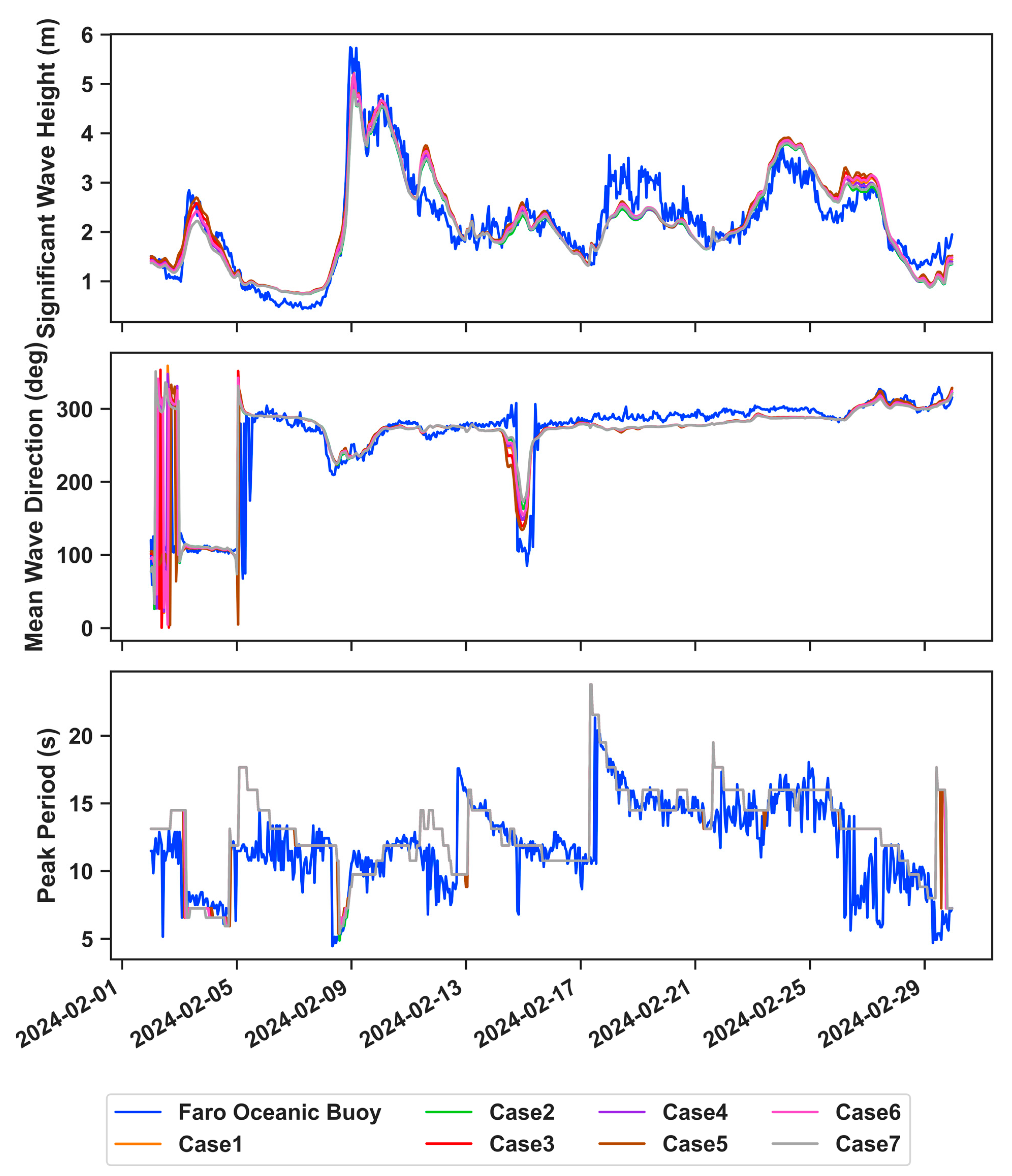
Figure A2.
Time series of Hs, Dir, and Tp for each model configuration during the calibration period (February 2024) at Cadiz Buoy.
Figure A2.
Time series of Hs, Dir, and Tp for each model configuration during the calibration period (February 2024) at Cadiz Buoy.
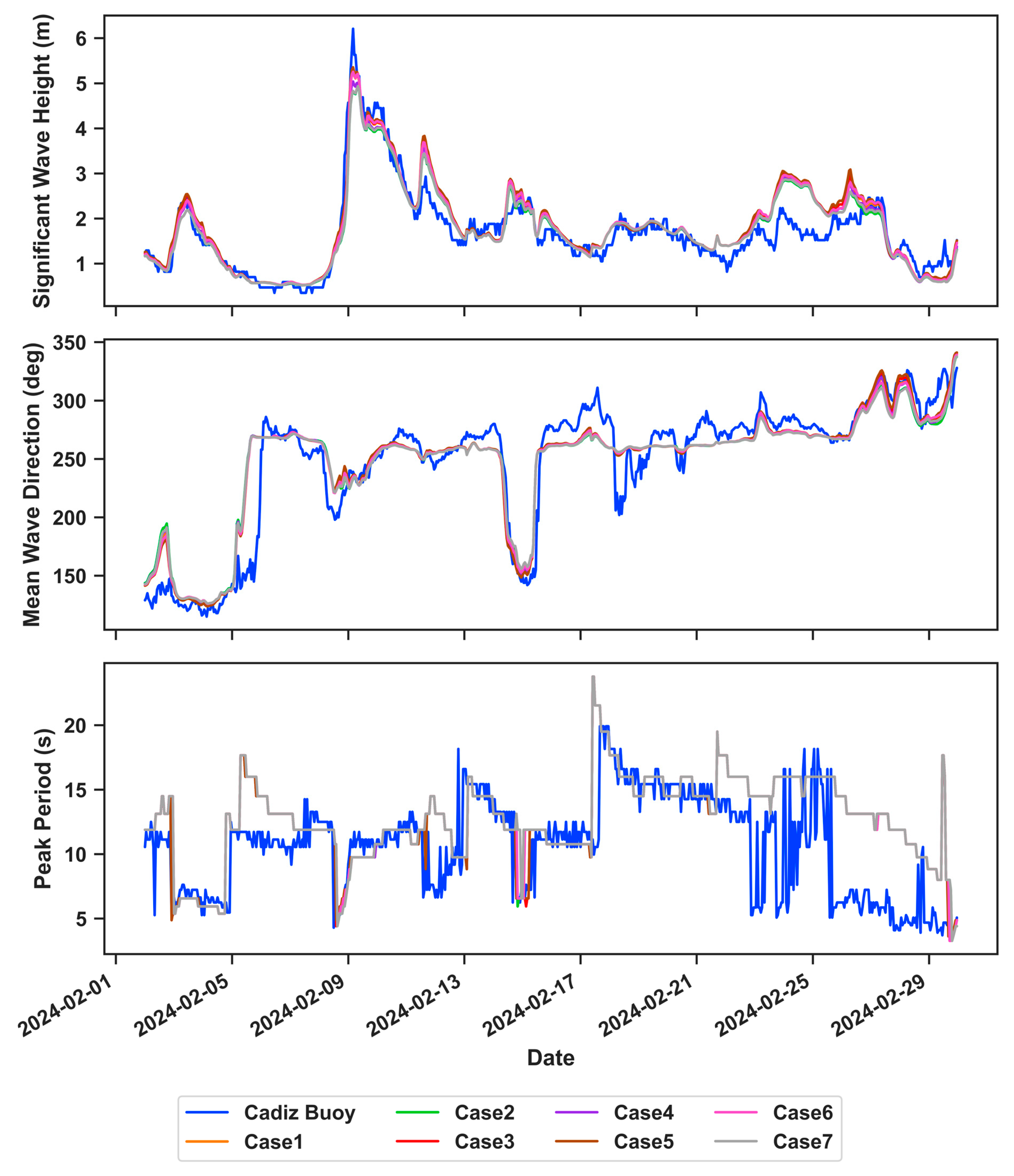
Figure A3.
Time series of Hs, Dir, and Tp for each model configuration during the calibration period (February 2024) at Sines Buoy.
Figure A3.
Time series of Hs, Dir, and Tp for each model configuration during the calibration period (February 2024) at Sines Buoy.
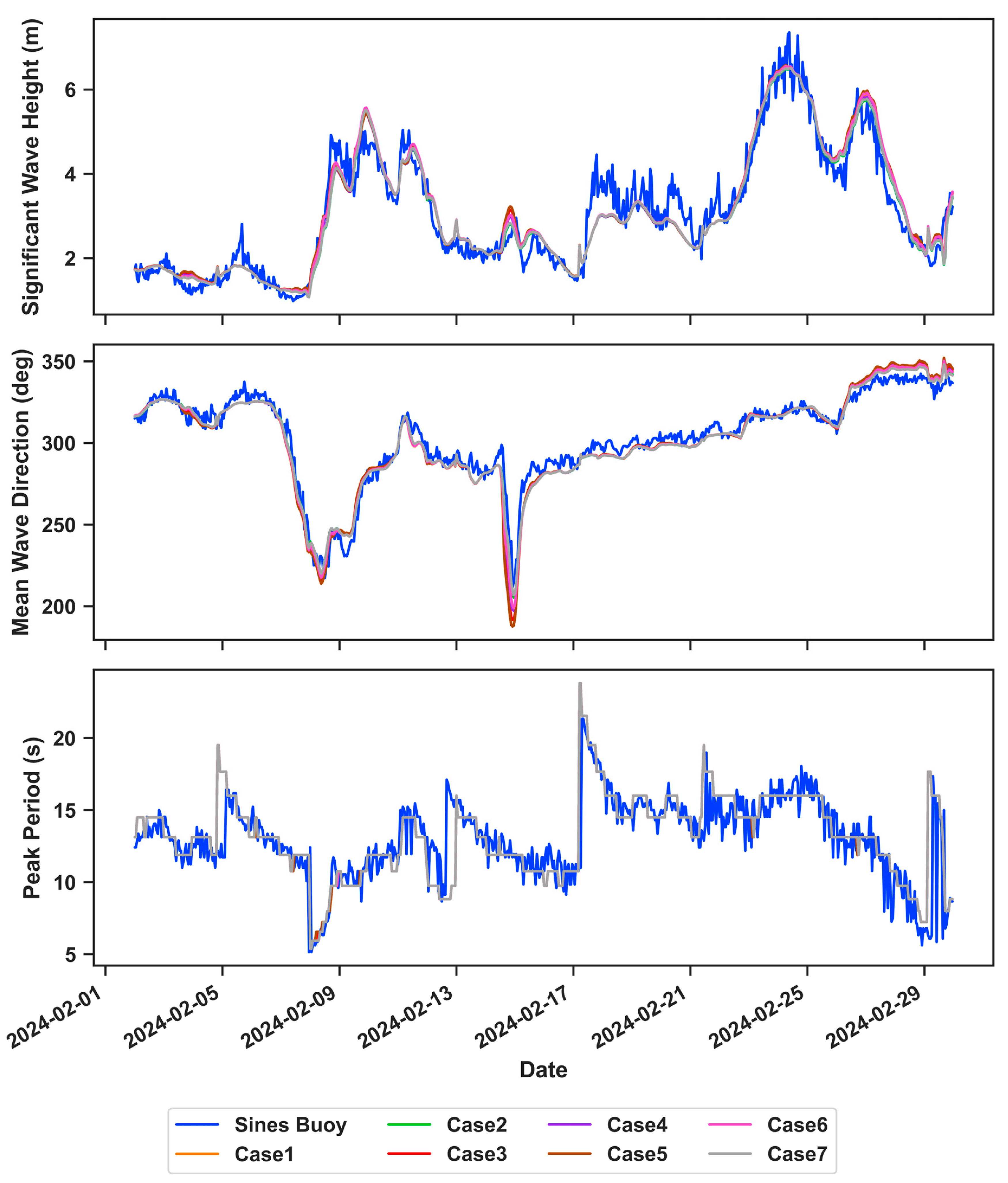

Table A1.
Error metrics of mean wave direction comparing model results of each calibration setting with buoy observations. Values in bold indicate the lowest (RMSE or BIAS) or highest (MSS or R) among all cases.
Table A1.
Error metrics of mean wave direction comparing model results of each calibration setting with buoy observations. Values in bold indicate the lowest (RMSE or BIAS) or highest (MSS or R) among all cases.
| Faro Ocean Buoy | Cadiz Buoy | Sines Buoy | ||||||||||
| RMSE (deg) | BIAS (deg) | MSS | R | RMSE (deg) | BIAS (deg) | MSS | R | RMSE (m) | BIAS (m) | MSS | R | |
| Case1 | 38.067 | 1.631 | 0.893 | 0.801 | 20.933 | 0.729 | 0.957 | 0.932 | 6.857 | -1.781 | 0.985 | 0.976 |
| Case2 | 41.279 | 3.578 | 0.865 | 0.760 | 21.722 | 0.318 | 0.953 | 0.927 | 6.058 | -1.641 | 0.988 | 0.979 |
| Case3 | 31.859 | -0.904 | 0.930 | 0.866 | 20.648 | 1.005 | 0.959 | 0.932 | 7.607 | -1.882 | 0.982 | 0.972 |
| Case4 | 37.551 | 1.481 | 0.895 | 0.806 | 21.276 | 0.638 | 0.956 | 0.929 | 6.751 | -1.755 | 0.985 | 0.976 |
| Case5 | 30.589 | -2.218 | 0.936 | 0.878 | 20.394 | 1.202 | 0.961 | 0.934 | 8.232 | -1.953 | 0.979 | 0.968 |
| Case6 | 37.340 | 1.282 | 0.897 | 0.809 | 20.718 | 0.684 | 0.958 | 0.934 | 6.700 | -1.823 | 0.986 | 0.977 |
| Case7 | 41.633 | 3.735 | 0.861 | 0.755 | 21.500 | 0.249 | 0.954 | 0.930 | 5.974 | -1.684 | 0.988 | 0.979 |
Table A2.
Error metrics of peak period comparing model results of each calibration setting with buoy observations. Values in bold indicate the lowest (RMSE or BIAS) or highest (MSS or R) among all cases.
Table A2.
Error metrics of peak period comparing model results of each calibration setting with buoy observations. Values in bold indicate the lowest (RMSE or BIAS) or highest (MSS or R) among all cases.
| Faro Buoy | Cadiz Buoy | Sines Buoy | ||||||||||
| RMSE (s) | BIAS (s) | MSS | R | RMSE (s) | BIAS (s) | MSS | R | RMSE (s) | BIAS (s) | MSS | R | |
| Case1 | 2.812 | 1.020 | 0.780 | 0.635 | 3.955 | 1.976 | 0.702 | 0.540 | 1.948 | 0.142 | 0.869 | 0.754 |
| Case2 | 2.839 | 1.034 | 0.776 | 0.628 | 3.958 | 1.998 | 0.700 | 0.540 | 1.947 | 0.144 | 0.869 | 0.754 |
| Case3 | 2.812 | 1.026 | 0.779 | 0.634 | 3.900 | 1.917 | 0.711 | 0.553 | 1.948 | 0.142 | 0.868 | 0.753 |
| Case4 | 2.812 | 1.021 | 0.780 | 0.635 | 3.955 | 1.978 | 0.701 | 0.540 | 1.948 | 0.142 | 0.869 | 0.754 |
| Case5 | 2.769 | 0.988 | 0.787 | 0.646 | 3.888 | 1.907 | 0.714 | 0.556 | 1.948 | 0.145 | 0.868 | 0.753 |
| Case6 | 2.806 | 1.033 | 0.781 | 0.637 | 3.985 | 2.025 | 0.697 | 0.535 | 1.945 | 0.150 | 0.869 | 0.755 |
| Case7 | 2.833 | 1.047 | 0.777 | 0.631 | 4.010 | 2.053 | 0.692 | 0.529 | 1.945 | 0.151 | 0.869 | 0.754 |
Table A3.
Sensitivity tests for directional spreading.
| Sensitivity Test | Directional Spreading | Simulation Timeframe |
| 1 | Degree E30 N30 S30 W40 | February 2024 |
| 2 | Degree E40 N40 S40 W40 | February 2024 |
| 3 | Power E2 N2 S3 W4 | February 2024 |
| 4 | Power E1.5 N1.5 S1.5 W1.5 | February 2024 |
| 5 | Power E2 N2 S3 W3 | February 2024 |
| 6 | Power E3 N3 S3 W3 | February 2024 |
| 7 | Power E15 N15 S15 W15 | February 2024 |
| 8 | Power E2 N4 S3 W4 | February 2024 |
| 9 | Power E4 N4 S4 W4 | February 2024 |
| 10 | Power E2 N2 S2 W4 | February 2024 |
| 11 | Power E2 N2 S2 W3 | February 2024 |
| 12 | Power E2 N2 S3 W4 | November 2023 |
| 13 | Power E2 N2 S2 W4 | November 2023 |
| 14 | Power E2 N2 S2 W3 | November 2023 |
| 15 | Power E2 N2 S2 W4 | 21-10-2023 – 07-11-2023 (westerly storm) |
| 16 | Power E2 N2 S2 W4 | 08-02-2023 – 22-02-2023 (easterly storm) |
Table A4.
Error metrics of significant wave height during the calibration period (February 2024). Directional spreading refers to values for directional spreading for each segment on each side (E = east, N = north, S = south, W = west). Simulation cases with the best metrics results are highlighted in bold.
| Faro Ocean Buoy | Cadiz Buoy | Sines Buoy | ||||||||||
| Directional Spreading | RMSE (m) | BIAS (m) | MSS | R | RMSE (m) | BIAS (m) | MSS | R | RMSE (m) | BIAS (m) | MSS | R |
| Degree E30 N30 S30 W40 | 0.404 | -0.070 | 0.955 | 0.916 | 0.370 | 0.082 | 0.958 | 0.923 | 0.421 | -0.022 | 0.978 | 0.956 |
| Degree E40 N40 S40 W40 | 0.415 | -0.027 | 0.952 | 0.908 | 0.424 | 0.154 | 0.945 | 0.907 | 0.398 | -0.025 | 0.980 | 0.960 |
| Power E2 N2 S3 W4 | 0.348 | -0.107 | 0.966 | 0.941 | 0.280 | -0.032 | 0.976 | 0.954 | 0.387 | 0.007 | 0.981 | 0.962 |
| Power E1.5 N1.5 S1.5 W1.5 | 0.390 | -0.050 | 0.958 | 0.920 | 0.374 | 0.103 | 0.957 | 0.923 | 0.401 | -0.014 | 0.980 | 0.960 |
| Power E2 N2 S3 W3 | 0.359 | -0.104 | 0.964 | 0.936 | 0.292 | -0.015 | 0.974 | 0.950 | 0.394 | 0.001 | 0.980 | 0.961 |
| Power E3 N3 S3 W3 | 0.359 | -0.102 | 0.964 | 0.936 | 0.291 | -0.013 | 0.974 | 0.950 | 0.410 | -0.001 | 0.979 | 0.959 |
| Power E15 N15 S15 W15 | 0.515 | -0.346 | 0.926 | 0.920 | 0.434 | -0.302 | 0.940 | 0.939 | 0.447 | -0.004 | 0.975 | 0.951 |
| Power E2 N4 S3 W4 | 0.349 | -0.104 | 0.966 | 0.940 | 0.279 | -0.031 | 0.976 | 0.954 | 0.414 | 0.003 | 0.979 | 0.958 |
| Power E4 N4 S4 W4 | 0.355 | -0.125 | 0.965 | 0.940 | 0.276 | -0.066 | 0.977 | 0.957 | 0.414 | 0.001 | 0.979 | 0.958 |
| Power E2 N2 S2 W4 | 0.346 | -0.072 | 0.967 | 0.939 | 0.297 | 0.026 | 0.973 | 0.948 | 0.388 | 0.009 | 0.981 | 0.962 |
| Power E2 N2 S2 W3 | 0.354 | -0.068 | 0.965 | 0.935 | 0.314 | 0.041 | 0.970 | 0.943 | 0.394 | 0.003 | 0.980 | 0.961 |
Table A5.
Error metrics of significant wave height during the validation period (November 2023). Directional spreading refers to values for directional spreading for each segment on each side (E = east, N = north, S = south, W = west). The simulation configuration with the best metrics results is highlighted in bold.
| Faro Ocean Buoy | Faro Coast Buoy | Cadiz Buoy | Sines Buoy | |||||||||||||
| Directional Spreading | RMSE | BIAS | MSS | R | RMSE | BIAS | MSS | R | RMSE | BIAS | MSS | R | RMSE | BIAS | MSS | R |
| E2 N2 S3 W4 | 0.341 | 0.058 | 0.956 | 0.93 | 0.217 | -0.145 | 0.950 | 0.947 | 0.251 | 0.054 | 0.957 | 0.942 | 0.335 | -0.024 | 0.989 | 0.982 |
| E2 N2 S2 W4 | 0.357 | 0.092 | 0.953 | 0.93 | 0.204 | -0.121 | 0.956 | 0.948 | 0.300 | 0.118 | 0.942 | 0.933 | 0.322 | -0.013 | 0.990 | 0.983 |
| E2 N2 S2 W3 | 0.368 | 0.101 | 0.950 | 0.922 | 0.183 | -0.093 | 0.964 | 0.951 | 0.328 | 0.149 | 0.931 | 0.925 | 0.328 | -0.022 | 0.990 | 0.983 |
Table A6.
Error metrics of significant wave height during the storm with westerly waves with the directional spreading set to power E2 N2 S2 W4.
Table A6.
Error metrics of significant wave height during the storm with westerly waves with the directional spreading set to power E2 N2 S2 W4.
| Level 1 SIMULATION 2023-10-21 12:00:00 - 2023-11-07 12:00:00 - WAVES COMING FROM WEST | ||||||||||||||||
| Faro Oceanic Buoy | Faro Coast Buoy | Cadiz Buoy | Sines Buoy | |||||||||||||
| RUN ID | RMSE (m) | BIAS (m) | MSS | R | RMSE (m) | BIAS (m) | MSS | R | RMSE (m) | BIAS (m) | MSS | R | RMSE (m) | BIAS (m) | MSS | R |
| 1 | 0.539 | 0.426 | 0.898 | 0.922 | 0.283 | -0.127 | 0.945 | 0.933 | 0.517 | 0.417 | 0.890 | 0.927 | 0.406 | -0.046 | 0.981 | 0.967 |
| 2 | 0.540 | 0.426 | 0.898 | 0.922 | 0.284 | -0.127 | 0.945 | 0.932 | 0.516 | 0.417 | 0.890 | 0.927 | 0.406 | -0.046 | 0.981 | 0.967 |
| 3 | 0.459 | 0.339 | 0.921 | 0.927 | 0.255 | 0.011 | 0.952 | 0.919 | 0.375 | 0.250 | 0.937 | 0.935 | 0.390 | 0.019 | 0.983 | 0.968 |
| 4 | 0.461 | 0.341 | 0.921 | 0.928 | 0.256 | 0.018 | 0.952 | 0.920 | 0.381 | 0.258 | 0.935 | 0.935 | 0.394 | 0.020 | 0.983 | 0.967 |
| 5 | 0.462 | 0.343 | 0.921 | 0.928 | 0.257 | 0.020 | 0.952 | 0.921 | 0.385 | 0.262 | 0.935 | 0.936 | 0.391 | -0.165 | 0.983 | 0.975 |
Table A7.
Error metrics of significant wave height during the storm with easterly waves with the directional spreading set to power E2 N2 S2 W4.
Table A7.
Error metrics of significant wave height during the storm with easterly waves with the directional spreading set to power E2 N2 S2 W4.
| Faro Oceanic Buoy | Faro Coast Buoy | Sines Buoy | ||||||||||
|---|---|---|---|---|---|---|---|---|---|---|---|---|
| RUN ID | RMSE (m) | BIAS (m) | MSS | R | RMSE (m) | BIAS (m) | MSS | R | RMSE (m) | BIAS (m) | MSS | R |
| 1 | 0.385 | -0.265 | 0.964 | 0.962 | 0.367 | -0.266 | 0.954 | 0.958 | 0.356 | 0.162 | 0.901 | 0.878 |
| 2 | 0.385 | -0.265 | 0.964 | 0.962 | 0.368 | -0.266 | 0.954 | 0.958 | 0.356 | 0.162 | 0.901 | 0.878 |
| 3 | 0.373 | -0.275 | 0.966 | 0.969 | 0.358 | -0.254 | 0.955 | 0.956 | 0.333 | 0.118 | 0.912 | 0.880 |
| 5 | 0.360 | -0.255 | 0.969 | 0.969 | 0.352 | -0.241 | 0.957 | 0.955 | 0.341 | 0.135 | 0.908 | 0.880 |
Figure A4.
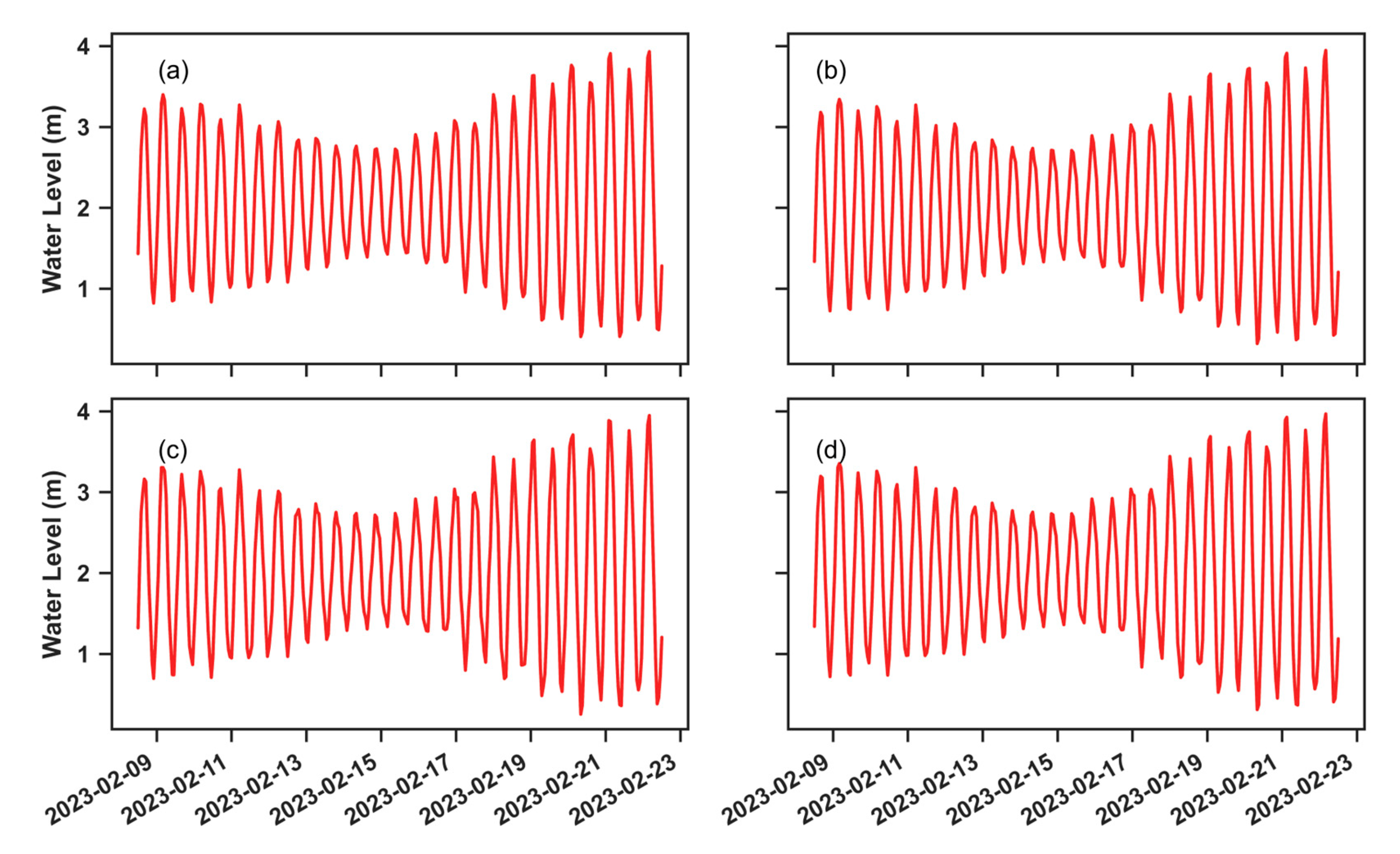
Time series of water levels at (a) Faro Ocean Buoy, (b) Faro Coast Buoy, (c) Cadiz Buoy, and (d) Sines Buoy during the storm with westerly waves (2023-10-21 – 2023-11-07).
Figure A4.
Time series of water levels at (a) Faro Ocean Buoy, (b) Faro Coast Buoy, (c) Cadiz Buoy, and (d) Sines Buoy during the storm with westerly waves (2023-10-21 – 2023-11-07).
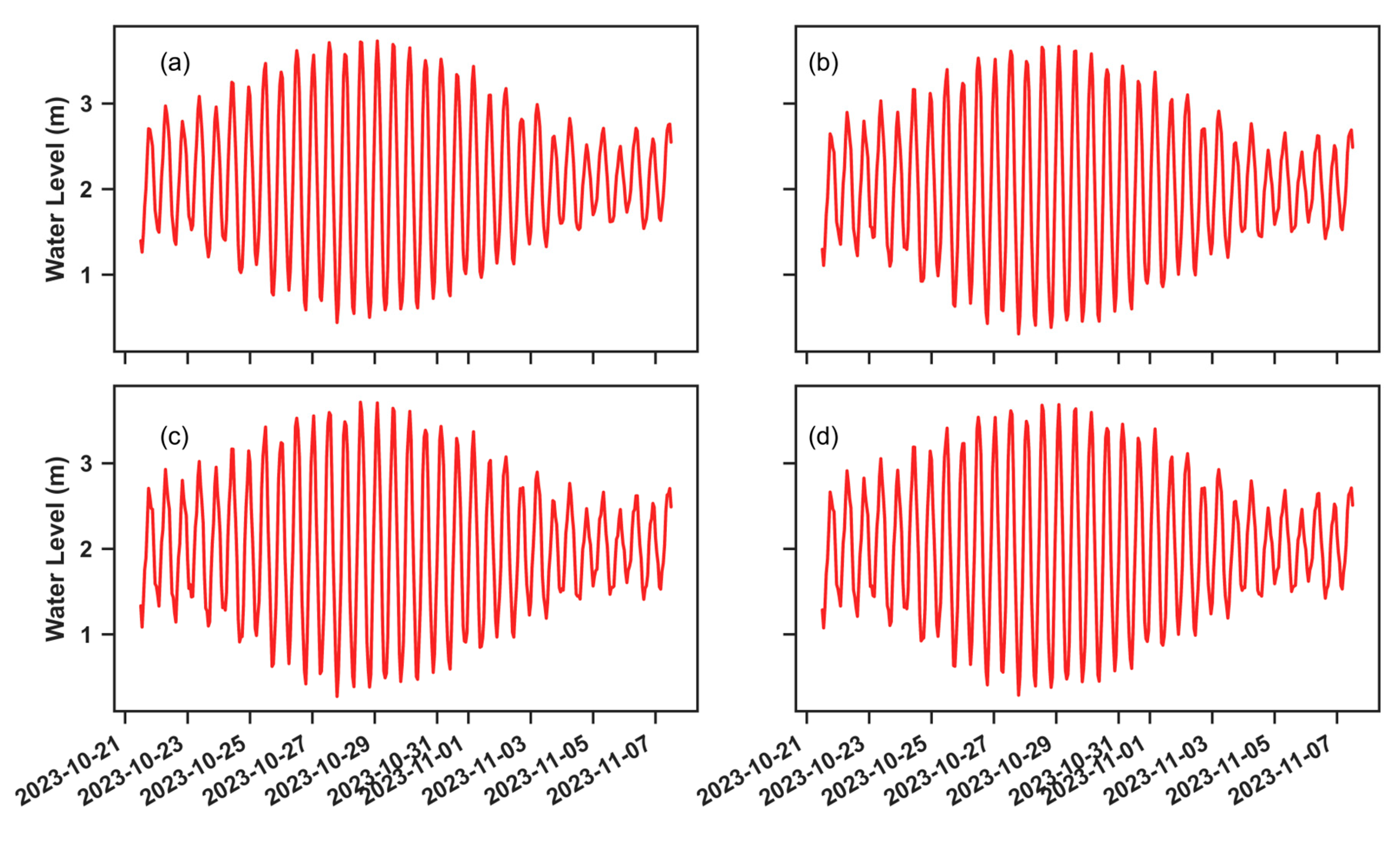
Figure A5.
Time series of water levels at (a) Faro Ocean Buoy, (b) Faro Coast Buoy, (c) Cadiz Buoy, and (d) Sines Buoy during the storm with easterly waves (2023-02-08 – 2023-02-22).
Figure A5.
Time series of water levels at (a) Faro Ocean Buoy, (b) Faro Coast Buoy, (c) Cadiz Buoy, and (d) Sines Buoy during the storm with easterly waves (2023-02-08 – 2023-02-22).
References
- Marsooli, R.; Orton, P.M.; Mellor, G.; Georgas, N.; Blumberg, A.F. A Coupled Circulation-Wave Model for Numerical Simulation of Storm Tides and Waves. J Atmos Ocean Technol 2017, 34, 1449–1467. [Google Scholar] [CrossRef]
- Calvino, C.; Dabrowski, T.; Dias, F. Current Interaction in Large-Scale Wave Models with an Application to Ireland. Cont Shelf Res 2022, 245. [Google Scholar] [CrossRef]
- Barnes, M.A.; Rautenbach, C. Toward Operational Wave-Current Interactions Over the Agulhas Current System. J Geophys Res Oceans 2020, 125. [Google Scholar] [CrossRef]
- Causio, S.; Ciliberti, S.A.; Clementi, E.; Coppini, G.; Lionello, P. A Modelling Approach for the Assessment of Wave-Currents Interaction in the Black Sea. J Mar Sci Eng 2021, 9. [Google Scholar] [CrossRef]
- Marechal, G.; Ardhuin, F. Surface Currents and Significant Wave Height Gradients: Matching Numerical Models and High-Resolution Altimeter Wave Heights in the Agulhas Current Region. J Geophys Res Oceans 2021, 126. [Google Scholar] [CrossRef]
- Causio, S.; Ciliberti, S.A.; Clementi, E.; Coppini, G.; Lionello, P. A Modelling Approach for the Assessment of Wave-Currents Interaction in the Black Sea. J Mar Sci Eng 2021, 9. [Google Scholar] [CrossRef]
- Clementi, E.; Oddo, P.; Drudi, M.; Pinardi, N.; Korres, G.; Grandi, A. Coupling Hydrodynamic and Wave Models: First Step and Sensitivity Experiments in the Mediterranean Sea. Ocean Dyn 2017, 67, 1293–1312. [Google Scholar] [CrossRef]
- Elahi, M.W.E.; Wang, X.H.; Salcedo-Castro, J.; Ritchie, E.A. Influence of Wave–Current Interaction on a Cyclone-Induced Storm Surge Event in the Ganges–Brahmaputra–Meghna Delta: Part 1—Effects on Water Level. J Mar Sci Eng 2023, 11. [Google Scholar] [CrossRef]
- Barnes, M.A.; Rautenbach, C. Toward Operational Wave-Current Interactions Over the Agulhas Current System. J Geophys Res Oceans 2020, 125. [Google Scholar] [CrossRef]
- Longuet-Higgins, M.S.; Stewart, R.W. Changes in the Form of Short Gravity Waves on Long Waves and Tidal Currents. J Fluid Mech 1960, 8, 565–583. [Google Scholar] [CrossRef]
- Wolf, J.; Prandle, D. Some Observations of Wave-Current Interaction; 1999; Vol. 37;
- Kumar, A.; Hayatdavoodi, M. On Wave–Current Interaction in Deep and Finite Water Depths. J Ocean Eng Mar Energy 2023, 9, 455–475. [Google Scholar] [CrossRef]
- Wang, X.H.; Elahi, M.W.E. Influence of Wave–Current Interaction on a Cyclone-Induced Storm-Surge Event in the Ganges-Brahmaputra-Meghna Delta: Part 2—Effects on Wave. J Mar Sci Eng 2023, 11. [Google Scholar] [CrossRef]
- Saruwatari, A.; Ingram, D.M.; Cradden, L. Wave-Current Interaction Effects on Marine Energy Converters. Ocean Engineering 2013, 73, 106–118. [Google Scholar] [CrossRef]
- Dietrich, J.C.; Tanaka, S.; Westerink, J.J.; Dawson, C.N.; Luettich, R.A.; Zijlema, M.; Holthuijsen, L.H.; Smith, J.M.; Westerink, L.G.; Westerink, H.J. Performance of the Unstructured-Mesh, SWAN+ ADCIRC Model in Computing Hurricane Waves and Surge. J Sci Comput 2012, 52, 468–497. [Google Scholar] [CrossRef]
- Silva, D.; Bento, A.R.; Martinho, P.; Guedes Soares, C. High Resolution Local Wave Energy Modelling in the Iberian Peninsula. Energy 2015, 91, 1099–1112. [Google Scholar] [CrossRef]
- Rusu, L.; Pilar, P.; Guedes Soares, C. Hindcast of the Wave Conditions along the West Iberian Coast. Coastal Engineering 2008, 55, 906–919. [Google Scholar] [CrossRef]
- Horta, J.; Oliveira, S.; Moura, D.; Ferreira, Ó. Nearshore Hydrodynamics at Pocket Beaches with Contrasting Wave Exposure in Southern Portugal. Estuar Coast Shelf Sci 2018, 204, 40–55. [Google Scholar] [CrossRef]
- Relvas, P.; Barton, E.D.; Dubert, J.; Oliveira, P.B.; Peliz, Á.; da Silva, J.C.B.; Santos, A.M.P. Physical Oceanography of the Western Iberia Ecosystem: Latest Views and Challenges. Prog Oceanogr 2007, 74, 149–173. [Google Scholar] [CrossRef]
- Peliz, Á.; Dubert, J.; Santos, A.M.P.; Oliveira, P.B.; Le Cann, B. Winter Upper Ocean Circulation in the Western Iberian Basin - Fronts, Eddies and Poleward Flows: An Overview. Deep Sea Res 1 Oceanogr Res Pap 2005, 52, 621–646. [Google Scholar] [CrossRef]
- Mills, L.; Janeiro, J.; Martins, F. Baseline Climatology of the Canary Current Upwelling System and Evolution of Sea Surface Temperature. Remote Sens (Basel) 2024, 16. [Google Scholar] [CrossRef]
- Álvarez-Salgado, X.A.; Figueiras, F.G.; Perez, F.F.; Groom, S.; Nogueira, E.; Borges, A. V.; Chou, L.; Castro, C.G.; Moncoiffé, G.; Rios, A.F.; et al. The Portugal Coastal Counter Current off NW Spain: New Insights on Its Biogeochemical Variability. Prog Oceanogr 2003, 56, 281–321. [Google Scholar] [CrossRef]
- Relvas, P.; Barton, E.D. Mesoscale Patterns in the Cape São Vicente (Iberian Peninsula) Upwelling Region. J Geophys Res Oceans 2002, 107. [Google Scholar] [CrossRef]
- Ferreira, Ó.; Kupfer, S.; Costas, S. Implications of Sea-Level Rise for Overwash Enhancement at South Portugal. Natural Hazards 2021, 109, 2221–2239. [Google Scholar] [CrossRef]
- Fernandes, M.; Fernandes, C.; Barroqueiro, T.; Agostinho, P.; Martins, ) N; Alonso-Martirena, A. Extreme Wave Height Events in Algarve (Portugal): Comparison between HF Radar Systems and Wave Buoys; 2018;
- Mota, P.; Pinto, J.P. Wave Energy Potential along the Western Portuguese Coast. Renew Energy 2014, 71, 8–17. [Google Scholar] [CrossRef]
- Ferreira, Ó.; Matias, A.; Pacheco, A. The East Coast of Algarve: A Barrier Island Dominated Coast. Thalassas 2016, 32, 75–85. [Google Scholar] [CrossRef]
- Booij, N.; Ris, R.C.; Holthuijsen, L.H. A Third-Generation Wave Model for Coastal Regions, Part I, Model Description and Validation A Third-Generation Wave Model for Coastal Regions 1. Model Description and Validation; 1999; Vol. 894;
- Booij, N.; Holthuijsen, L.H.; Ris, R.C. THE “SWAN” WAVE MODEL FOR SHALLOW WATER; 1996;
- Rogers, E.W.; Babanin, A. V.; Wang, D.W. Observation-Consistent Input and Whitecapping Dissipation in a Model for Wind-Generated Surface Waves: Description and Simple Calculations. J Atmos Ocean Technol 2012, 29, 1329–1346. [Google Scholar] [CrossRef]
- Janeiro, J.; Neves, A.; Martins, F.; Relvas, P. Integrating Technologies for Oil Spill Response in the SW Iberian Coast. Journal of Marine Systems 2017, 173, 31–42. [Google Scholar] [CrossRef]
- Martins, F.; Leitão, P.; Silva, A.; Neves, R. 3D Modelling in the Sado Estuary Using a New Generic Vertical Discretization Approach; 2001;
- Braunschweig, F.; Leitao, P.C.; Fernandes, L.; Pina, P.; Neves, R.J.J. The Object Oriented Design of the Integrated Water Modelling System MOHID; 2004;
- Mendonça, F.; Martins, F.; Janeiro, J. SMS-Coastal, a New Python Tool to Manage MOHID-Based Coastal Operational Models. J Mar Sci Eng 2023, 11. [Google Scholar] [CrossRef]
- Kallos, G.; Nickovic, S.; Papadopoulos, A.; Jovic, D.; Kakaliagou, O.; Misirlis, N.; Boukas, L.; Mitikou, N.; Sakellaridis, G.; Papageorgiou, J.; et al. The Regional Weather Forecasting System SKIRON: An Overview. In Proceedings of the Proceedings of the International Symposium on Regional Weather Prediction on Parallel Computer Environments; Athens, Greece, October 1997; pp. 109–122.
- Toledano, C.; Ghantous, M.; Lorente, P.; Dalphinet, A.; Aouf, L.; Sotillo, M.G. Impacts of an Altimetric Wave Data Assimilation Scheme and Currents-Wave Coupling in an Operational Wave System: The New Copernicus Marine IBI Wave Forecast Service. J Mar Sci Eng 2022, 10. [Google Scholar] [CrossRef]
- Gomez, B.; Aouf, L.; Dalphinet, A.; Louis, L.; Alonso, A.; Garcia, M.; Valdecasas, J.M.; Ciliberti, S.; Aznar, R.; Sotillo, M.G. Atlantic-Iberian Biscay Irish-IBI Production Centre IBI_ANALYSISFORECAST_WAV_005_005;
- Zhang, W.; Zhao, H.; Chen, G.; Yang, J. Assessing the Performance of SWAN Model for Wave Simulations in the Bay of Bengal. Ocean Engineering 2023, 285. [Google Scholar] [CrossRef]
- Edwards, K.L.; Rogers, W.E.; Siqueira, S.; Gay, P.; Wood, K. A Cost-Benefit Analysis of SWAN with Source Term Package ST6; 2018;
- SWAN Team Swanuse. 2020.
- Cavaleri, L.; Bertotti, L. The Miami 1981 Wave Model Intercomparison Test. Il Nuovo Cimento C 1982, 5, 159–188. [Google Scholar] [CrossRef]
- Ardhuin, F.; Rogers, E.; Babanin, A. V.; Filipot, J.F.; Magne, R.; Roland, A.; van der Westhuysen, A.; Queffeulou, P.; Lefevre, J.M.; Aouf, L.; et al. Semiempirical Dissipation Source Functions for Ocean Waves. Part I: Definition, Calibration, and Validation. J Phys Oceanogr 2010, 40, 1917–1941. [Google Scholar] [CrossRef]
- Zieger, S.; Babanin, A. V.; Erick Rogers, W.; Young, I.R. Observation-Based Source Terms in the Third-Generation Wave Model WAVEWATCH. Ocean Model (Oxf) 2015, 96, 2–25. [Google Scholar] [CrossRef]
- Wehde, H.; Schuckmann, K. V; Pouliquen, S.; Grouazel, A.; Bartolome, T.; Tintore, J.; De, M.; Alonso-Munoyerro, A.; Carval, T.; Racapé, V. In Situ TAC Multiparameter Products: INSITU_GLO_PHYBGCWAV_DISCRETE_MYNRT_013_030 INSITU_ARC_PHYBGCWAV_DISCRETE_MYNRT_013_031 INSITU_BAL_PHYBGCWAV_DISCRETE_MYNRT_013_032 INSITU_IBI_PHYBGCWAV_DISCRETE_MYNRT_013_033 INSITU_BLK_PHYBGCWAV_DISCRETE_MYNRT_013_034 INSITU_MED_PHYBGCWAV_DISCRETE_MYNRT_013_035 INSITU_NWS_PHYBGCWAV_DISCRETE_MYNRT_013_036 Issue: 2.4; 2024;
- O’Donncha, F.; Hartnett, M.; Nash, S.; Ren, L.; Ragnoli, E. Characterizing Observed Circulation Patterns within a Bay Using HF Radar and Numerical Model Simulations. Journal of Marine Systems 2015, 142, 96–110. [Google Scholar] [CrossRef]
- Willmott, C.I. ON THE VALIDATION OF MODELS. Phys Geogr 1981, 2, 184–194. [Google Scholar] [CrossRef]
- Majidi, A.G.; Ramos, V.; Amarouche, K.; Rosa Santos, P.; das Neves, L.; Taveira-Pinto, F. Assessing the Impact of Wave Model Calibration in the Uncertainty of Wave Energy Estimation. Renew Energy 2023, 212, 415–429. [Google Scholar] [CrossRef]
- Aydoğan, B.; Ayat, B. Performance Evaluation of SWAN ST6 Physics Forced by ERA5 Wind Fields for Wave Prediction in an Enclosed Basin. Ocean Engineering 2021, 240. [Google Scholar] [CrossRef]
- Sapiega, P.; Zalewska, T.; Struzik, P. Application of SWAN Model for Wave Forecasting in the Southern Baltic Sea Supplemented with Measurement and Satellite Data. Environmental Modelling and Software 2023, 163. [Google Scholar] [CrossRef]
Figure 1.
Map of the study area highlighting the general circulation patterns relative to the study. The Portugal Current and Azores Current that occur year-round are highlighted in grey. The Portugal Current propagates southward until it merges with the Canary Current along the west coast of Africa, but can occasionally turn eastward at Cape São Vicente (dark blue arrow). The winter circulation pattern of the Portugal Coastal Countercurrent that propagates northward at Cape São Vicente is highlighted in dark blue.
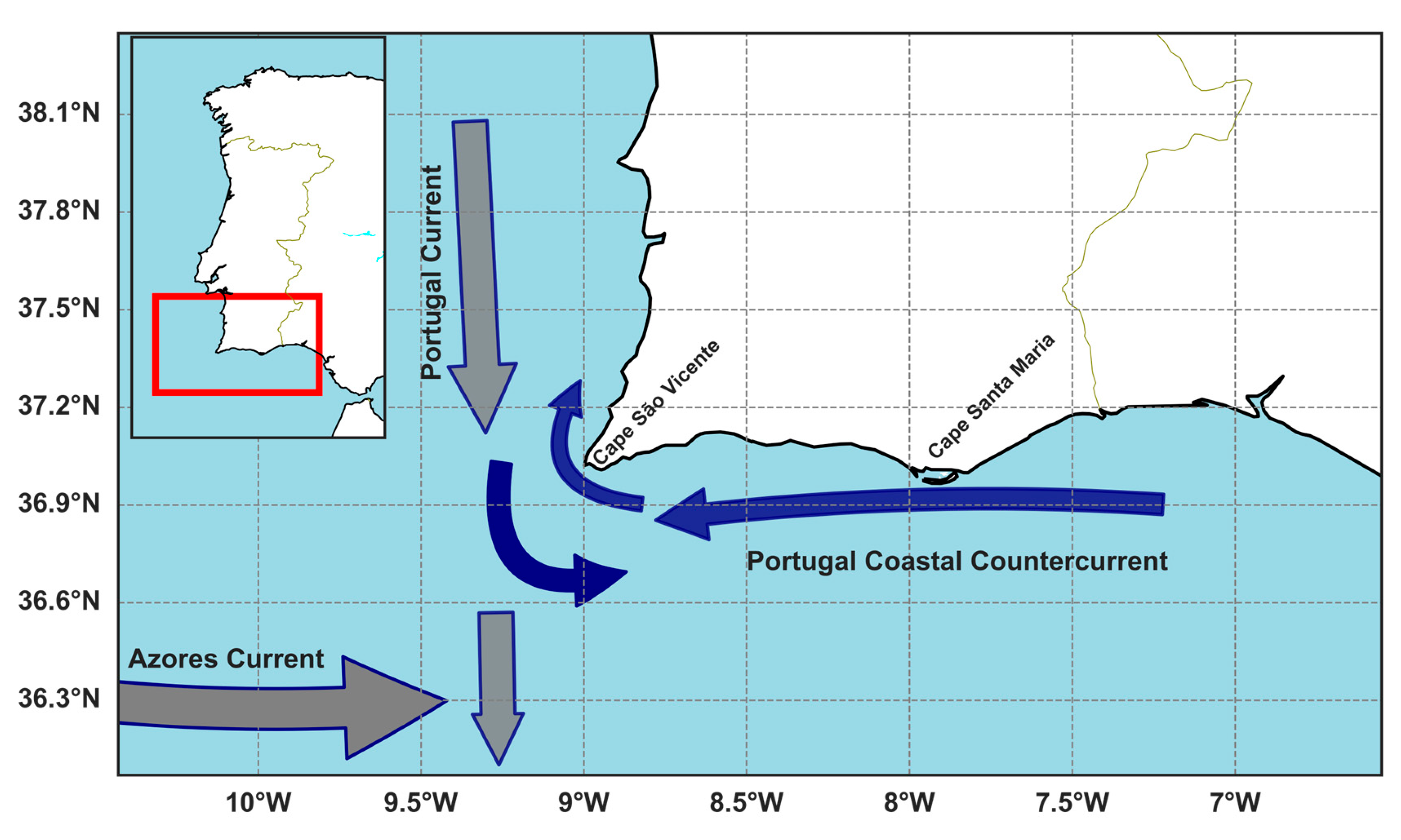
Figure 2.
Bathymetry of the computational grid. Buoy locations used for model calibration and validation are shown in red.
Figure 2.
Bathymetry of the computational grid. Buoy locations used for model calibration and validation are shown in red.
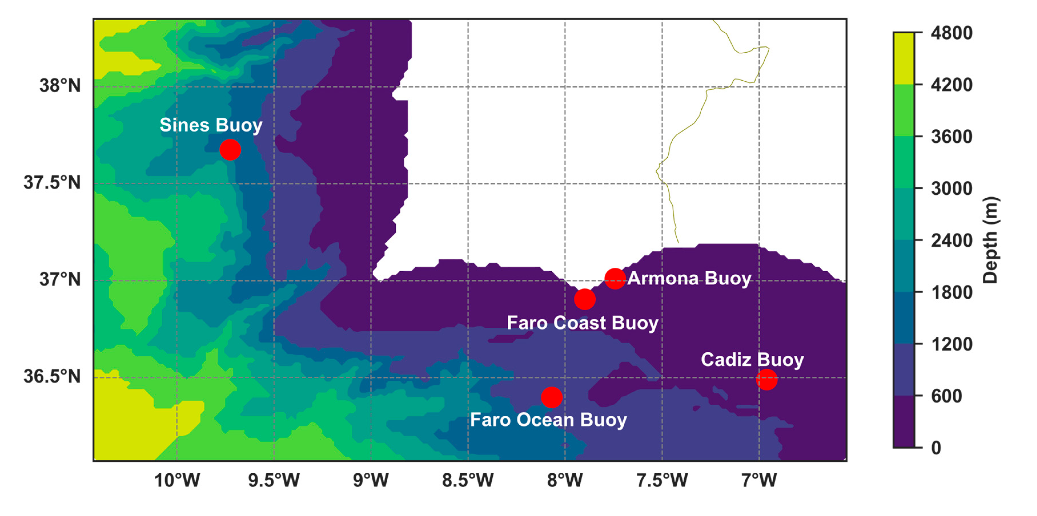
Figure 3.
Time series of Hs at (a) Faro Ocean Buoy, (b) Cadiz Buoy, and (c) Sines Buoy during the model calibration period. The black line represents the significant wave height of in-situ buoy observations (left axis). The shaded region represents the range of relative error between all modeled results and buoy observations (right axis), spanning from the minimum to the maximum percentage at each timestep (envelope of the seven runs in Table 3). Overpredictions of Hs are highlighted in red and underpredictions of Hs are highlighted in blue.
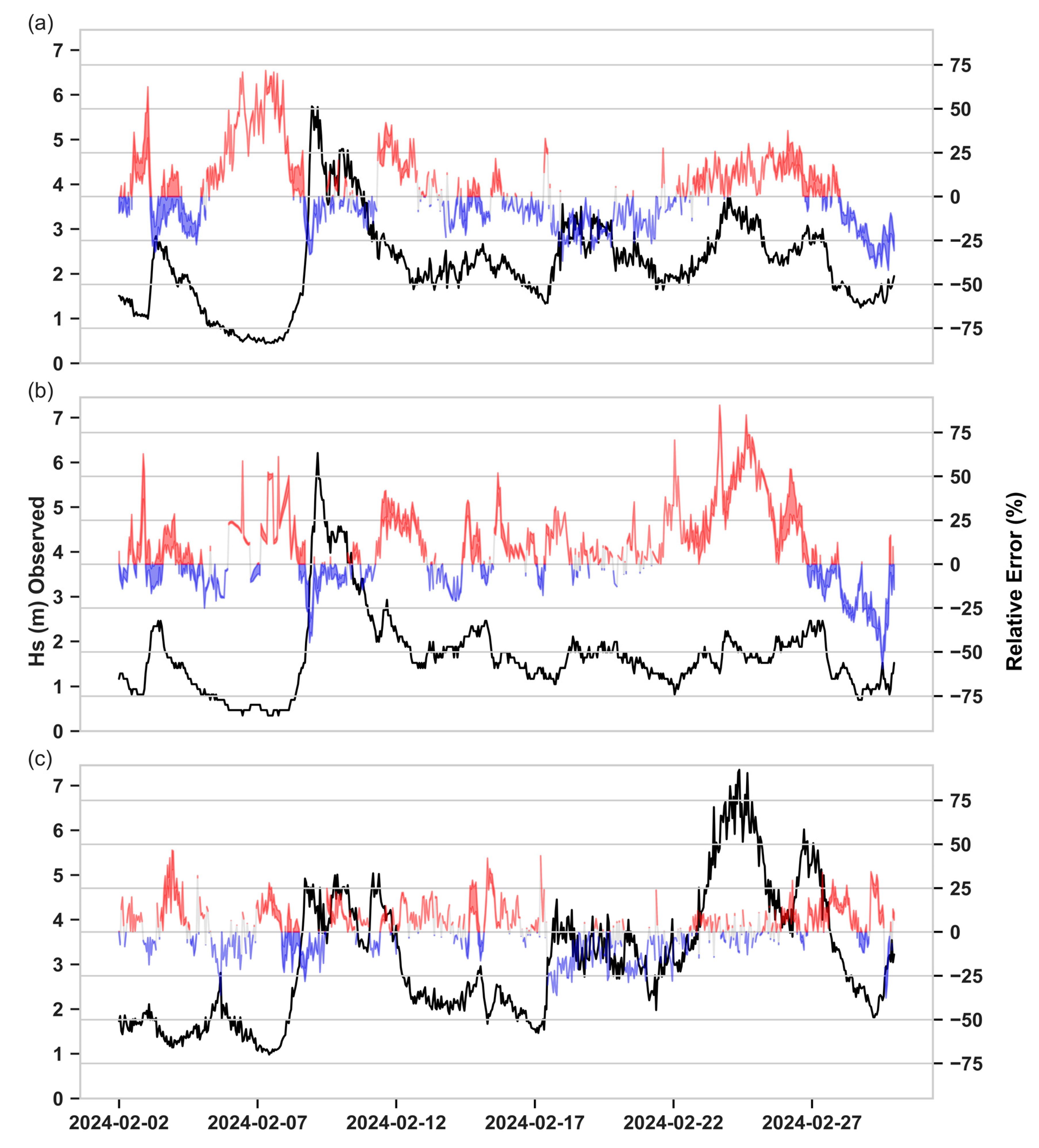
Figure 4.
Scatter plots showing the correlation between observations and modeled Hs at (a) Faro Ocean Buoy, (b) Faro Coast Buoy, (c) Cadiz Buoy, and (d) Sines Buoy.
Figure 4.
Scatter plots showing the correlation between observations and modeled Hs at (a) Faro Ocean Buoy, (b) Faro Coast Buoy, (c) Cadiz Buoy, and (d) Sines Buoy.
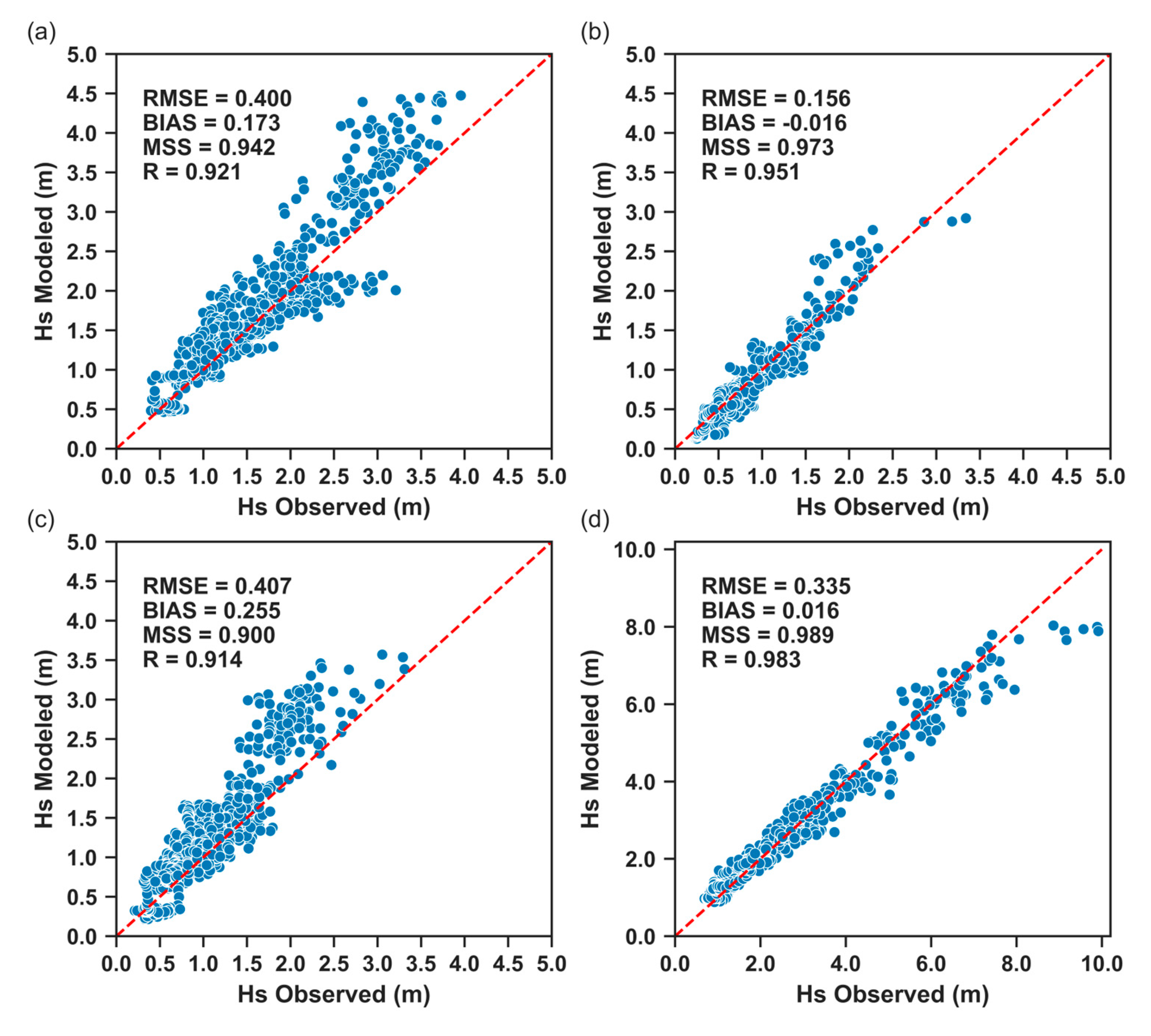
Figure 5.
Time series of significant wave height during a storm with waves coming from W-SW at (a) Faro Ocean Buoy, (b) Faro Coast Buoy, (c) Cadiz Buoy, and (d) Sines Buoy. The black line represents the significant wave height of in-situ buoy observations (left axis). The shaded region represents the range of relative error between all modeled results and buoy observations (right axis), spanning from the minimum to the maximum percentage at each timestep (envelope of the six runs in Table 3). Overpredictions of Hs are highlighted in red and underpredictions of Hs are highlighted in blue.
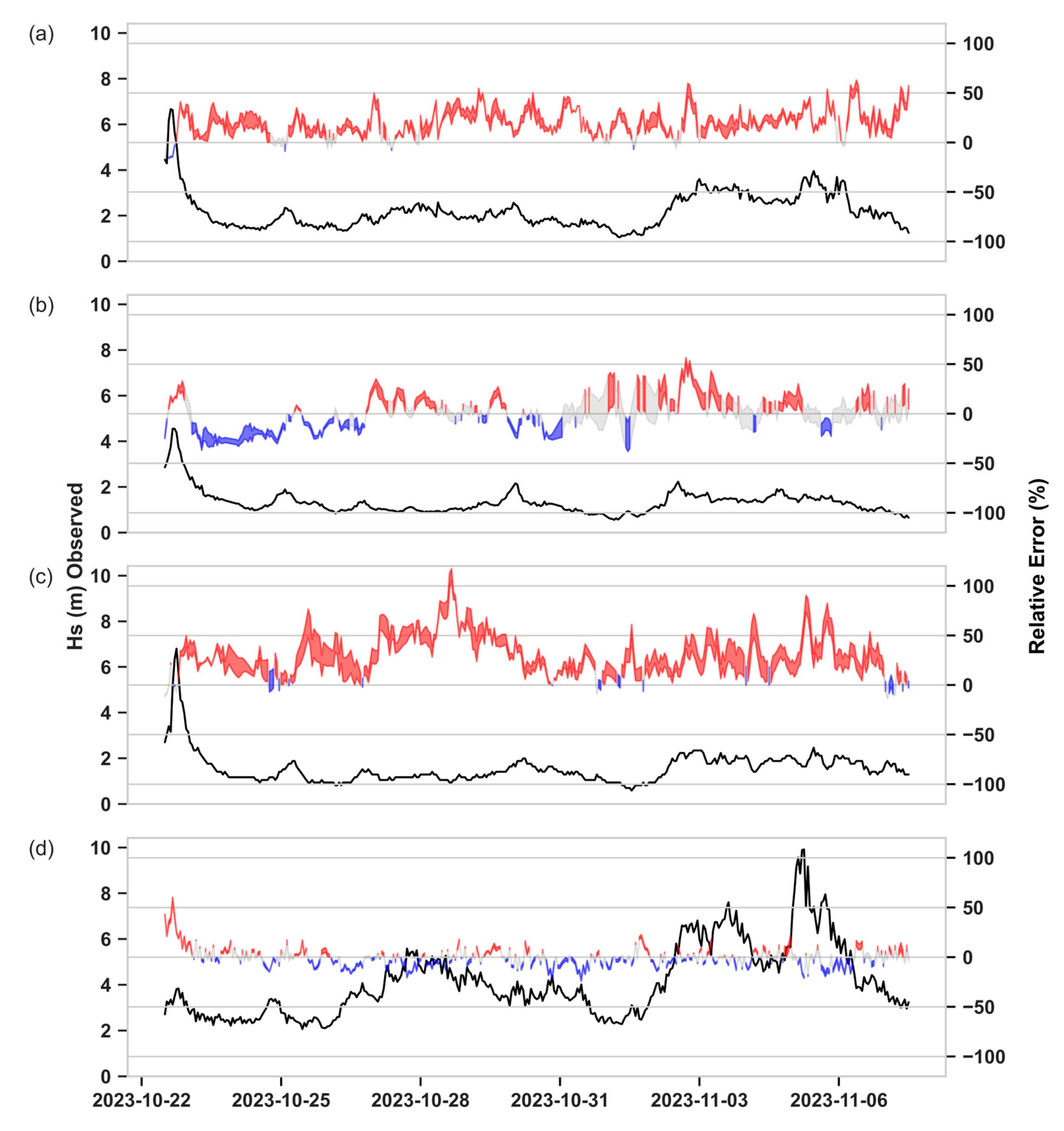
Figure 6.
2D spatial maps depicting the change in mean significant wave height by subtracting the run with no hydrodynamic input from (a) the SWAN run with SOMA surface current velocity and water level forcing, (b) the SWAN run with SOMA 10 m depth-averaged current velocity and water level forcing, (c) the SWAN run with SOMA 20 m depth-averaged current velocity and water level forcing, and (d) the SWAN run with SOMA full depth-averaged current velocity and water level forcing during the storm with waves coming form W-SW. The black arrows represent the mean current velocity direction and the green arrows represent the mean wave direction during the W-SW storm.
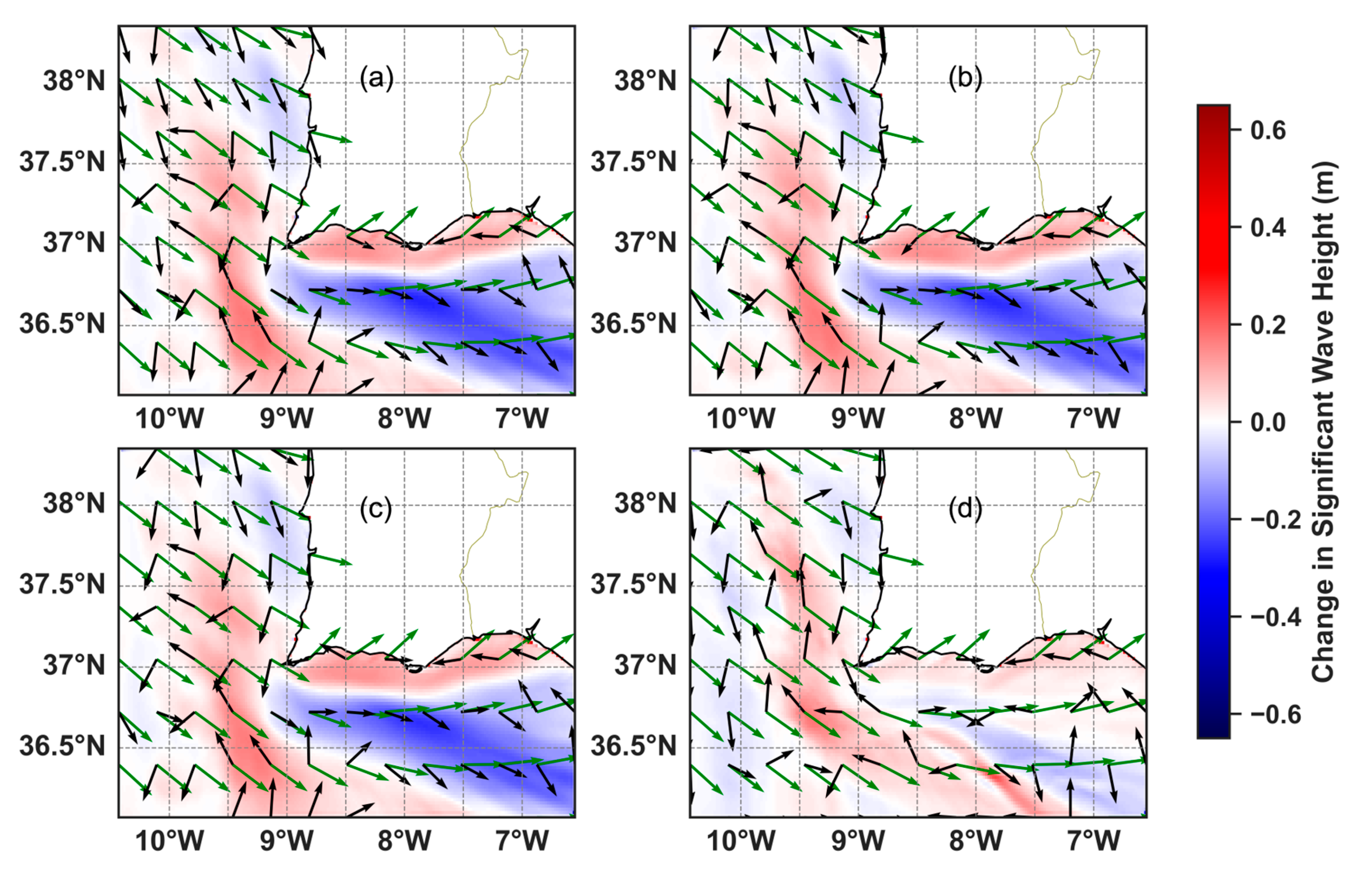
Figure 7.
Time series of SOMA current velocities at the locations of: (a) Faro Ocean Buoy, (b) Faro Coast Buoy, (c) Cadiz Buoy, and (d) Sines Buoy during the storm with westerly waves (2023-10-21 – 2023-11-07).
Figure 7.
Time series of SOMA current velocities at the locations of: (a) Faro Ocean Buoy, (b) Faro Coast Buoy, (c) Cadiz Buoy, and (d) Sines Buoy during the storm with westerly waves (2023-10-21 – 2023-11-07).
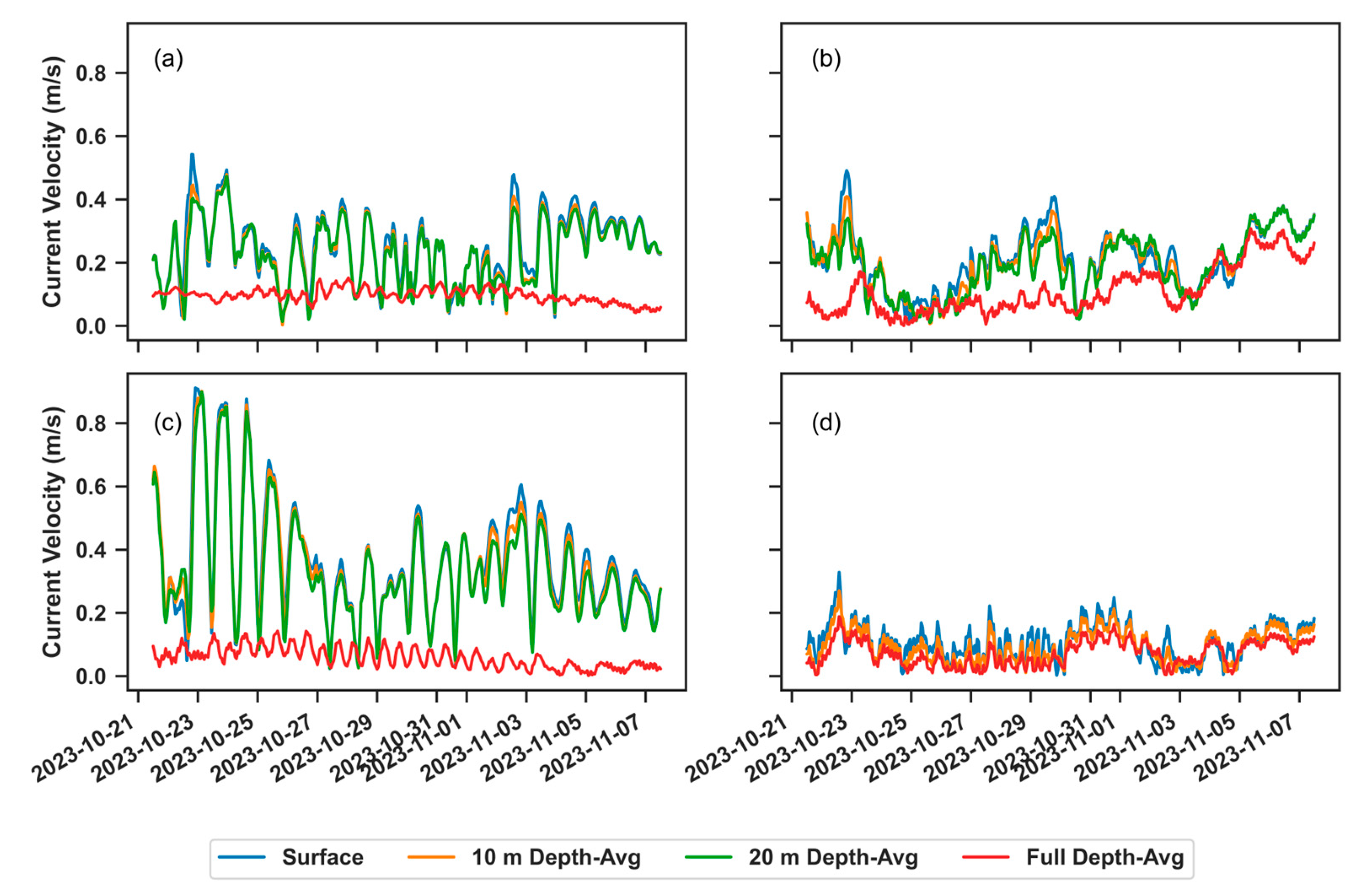
Figure 8.
Time series of significant wave height during a storm with waves coming from E-SE at (a) Faro Ocean Buoy, (b) Faro Coast Buoy, and (c) Sines Buoy. The black line represents the significant wave height of in-situ buoy observations (left axis). The shaded region represents the range of relative error between all modeled results and buoy observations (right axis), spanning from the minimum to the maximum percentage at each timestep (envelope of the seven runs in Table 3). Overpredictions of Hs are highlighted in red and underpredictions of Hs are highlighted in blue.
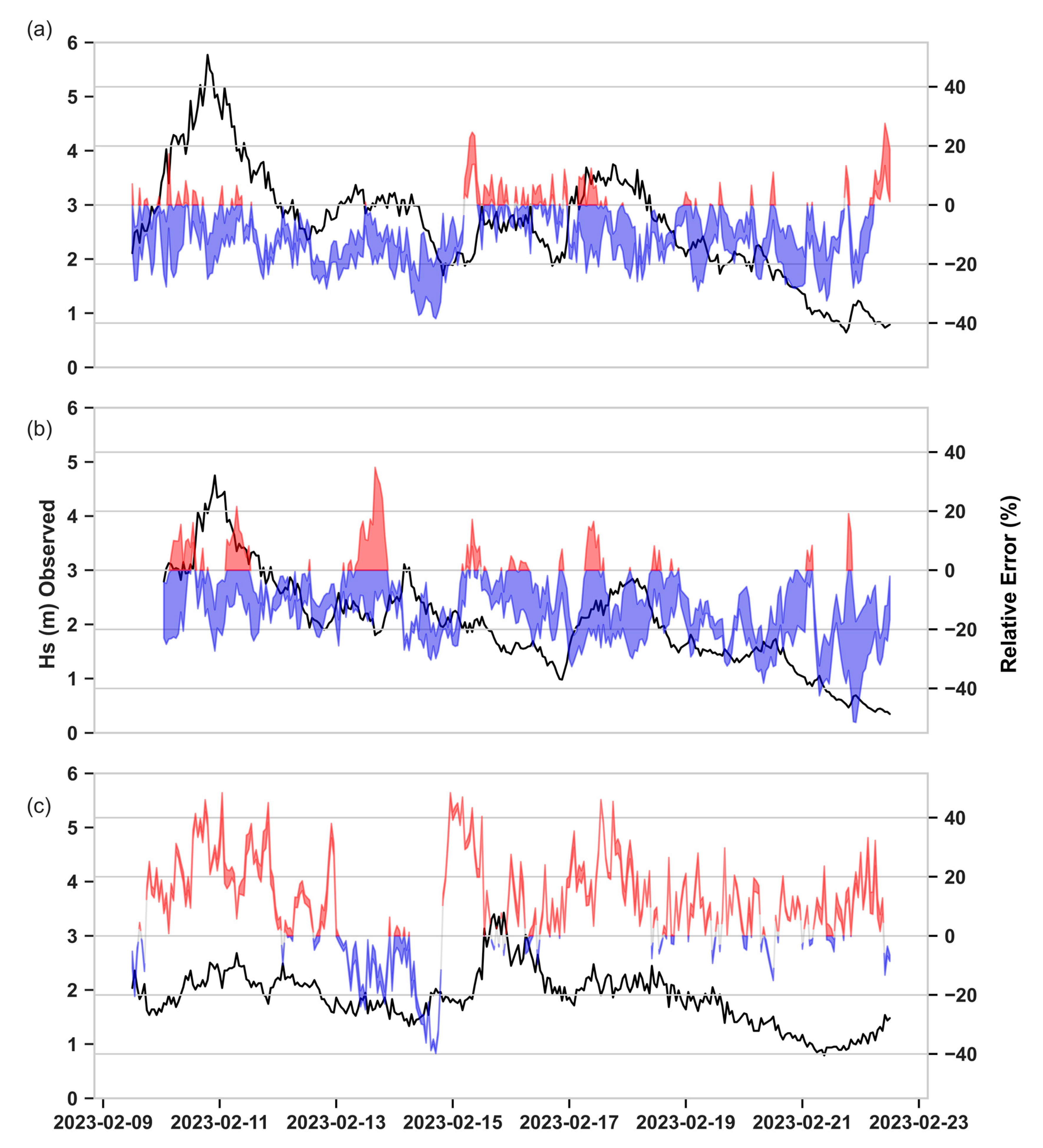
Figure 9.
2D spatial maps depicting the change in mean significant wave height by subtracting the run with no hydrodynamic input from (a) the SWAN run with SOMA surface current velocity and water level forcing, (b) the SWAN run with SOMA 10 m depth-averaged current velocity and water level forcing, (c) the SWAN run with SOMA 20 m depth-averaged current velocity and water level forcing, and (d) the SWAN run with SOMA full depth-averaged current velocity and water level forcing during the storm with waves coming from E-SE. The black arrows represent the mean current velocity direction and the green arrows represent the mean wave direction during the E-SE storm.
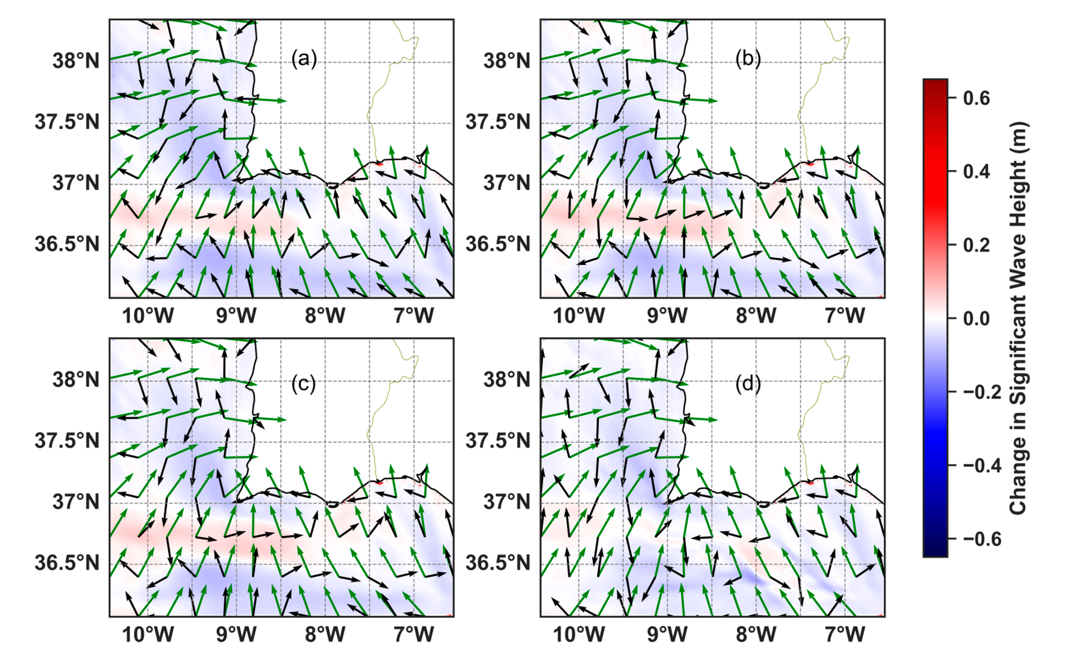
Figure 10.
Time series of SOMA current velocities at the locations of (a) Faro Ocean Buoy, (b) Faro Coast Buoy, (c) Cadiz Buoy, and (d) Sines Buoy during the storm with easterly waves (2023-02-08 – 2023-02-22).
Figure 10.
Time series of SOMA current velocities at the locations of (a) Faro Ocean Buoy, (b) Faro Coast Buoy, (c) Cadiz Buoy, and (d) Sines Buoy during the storm with easterly waves (2023-02-08 – 2023-02-22).
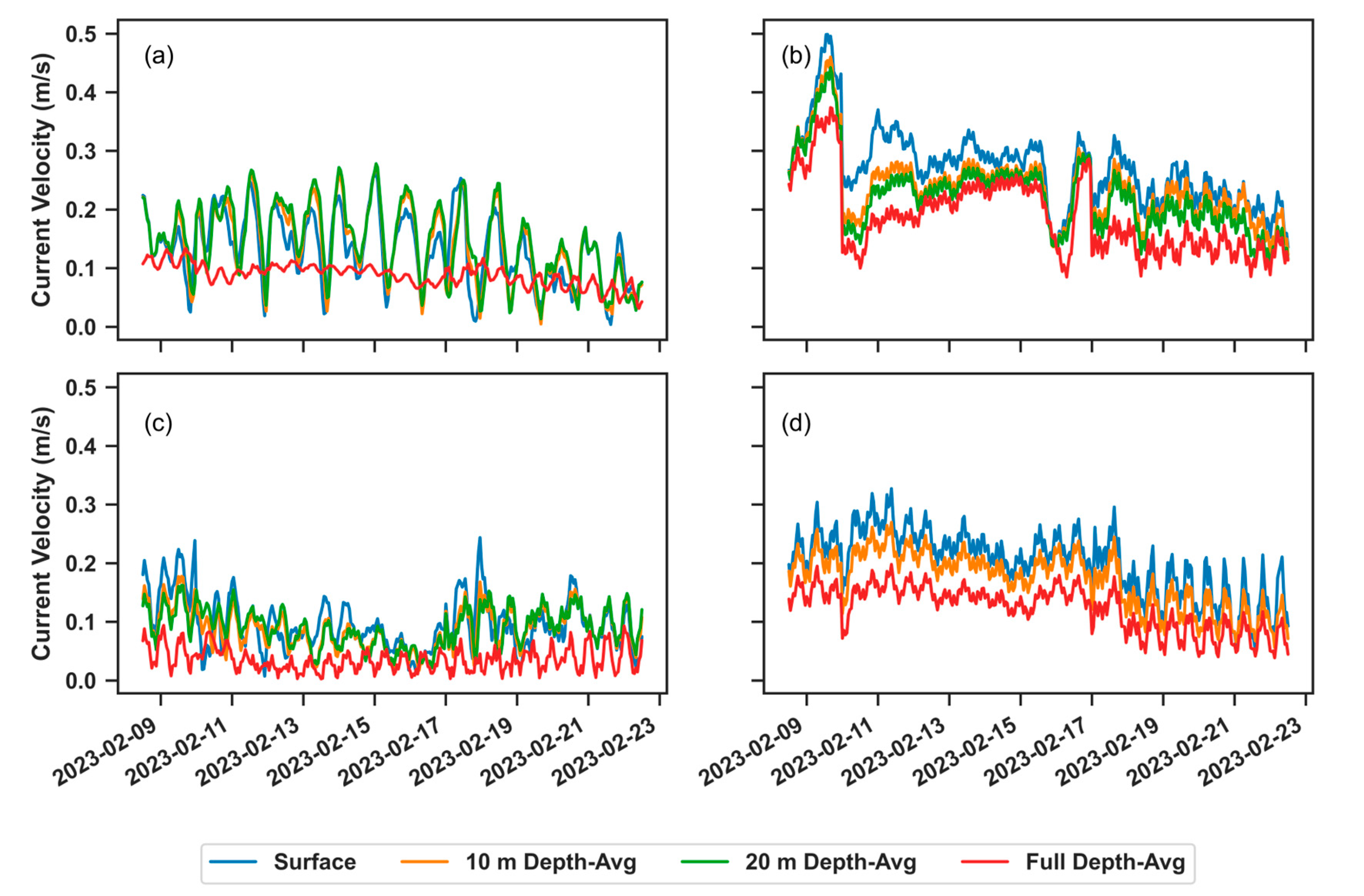
Figure 11.
Time series of significant wave height at Armona Buoy. The black line represents the significant wave height of in-situ buoy observations (left axis). The shaded region represents the range of relative error between all modeled results and buoy observations (right axis), spanning from the minimum to the maximum percentage at each timestep (envelope of the seven runs in Table 3). Overpredictions of Hs are highlighted in red and underpredictions of Hs are highlighted in blue. The green line represents the tidal level (from SOMA), with the high and low tides marked with the vertical dashed line.
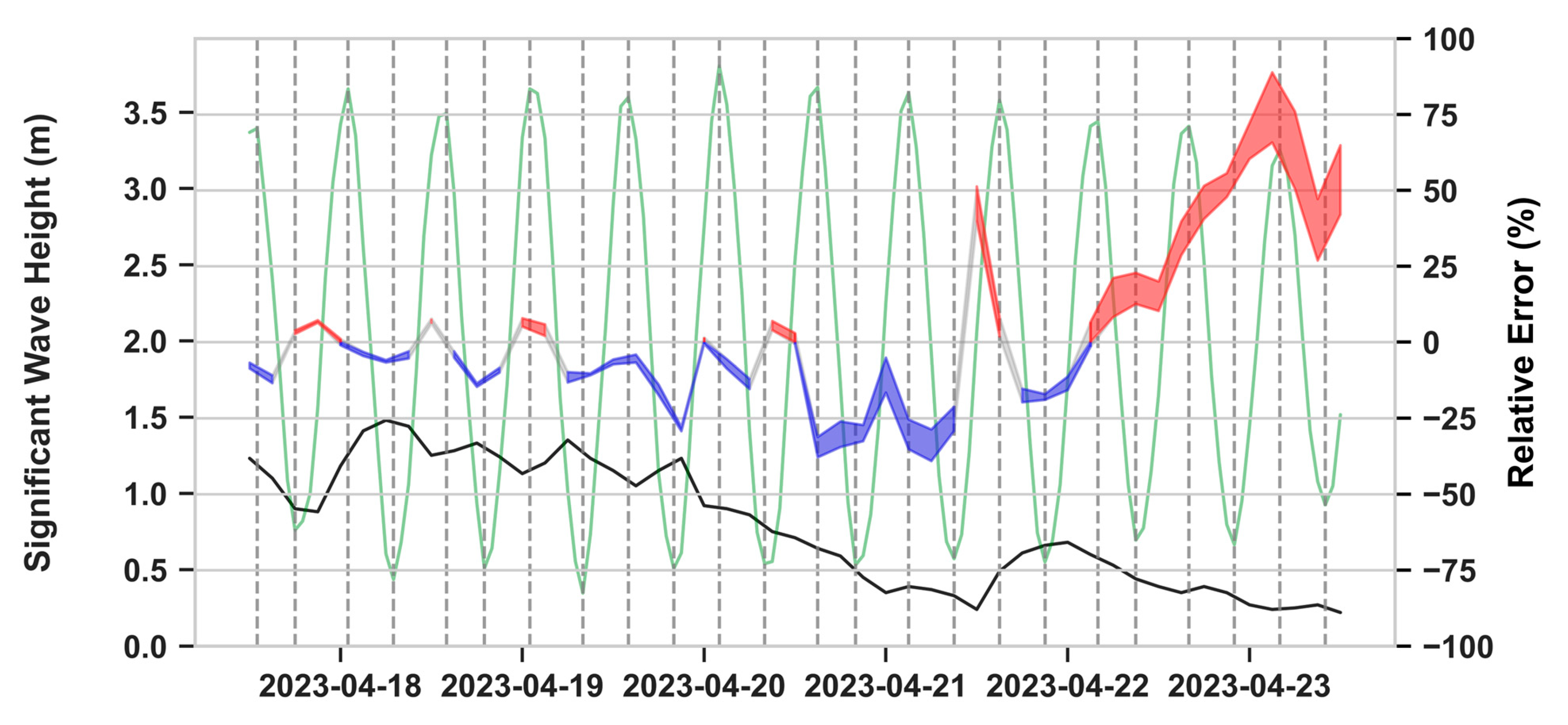
Figure 12.
Changes in Hs due to the combination of wave-current angle difference and surface current velocity magnitude for the (a) westerly storm and (b) easterly storm.
Figure 12.
Changes in Hs due to the combination of wave-current angle difference and surface current velocity magnitude for the (a) westerly storm and (b) easterly storm.
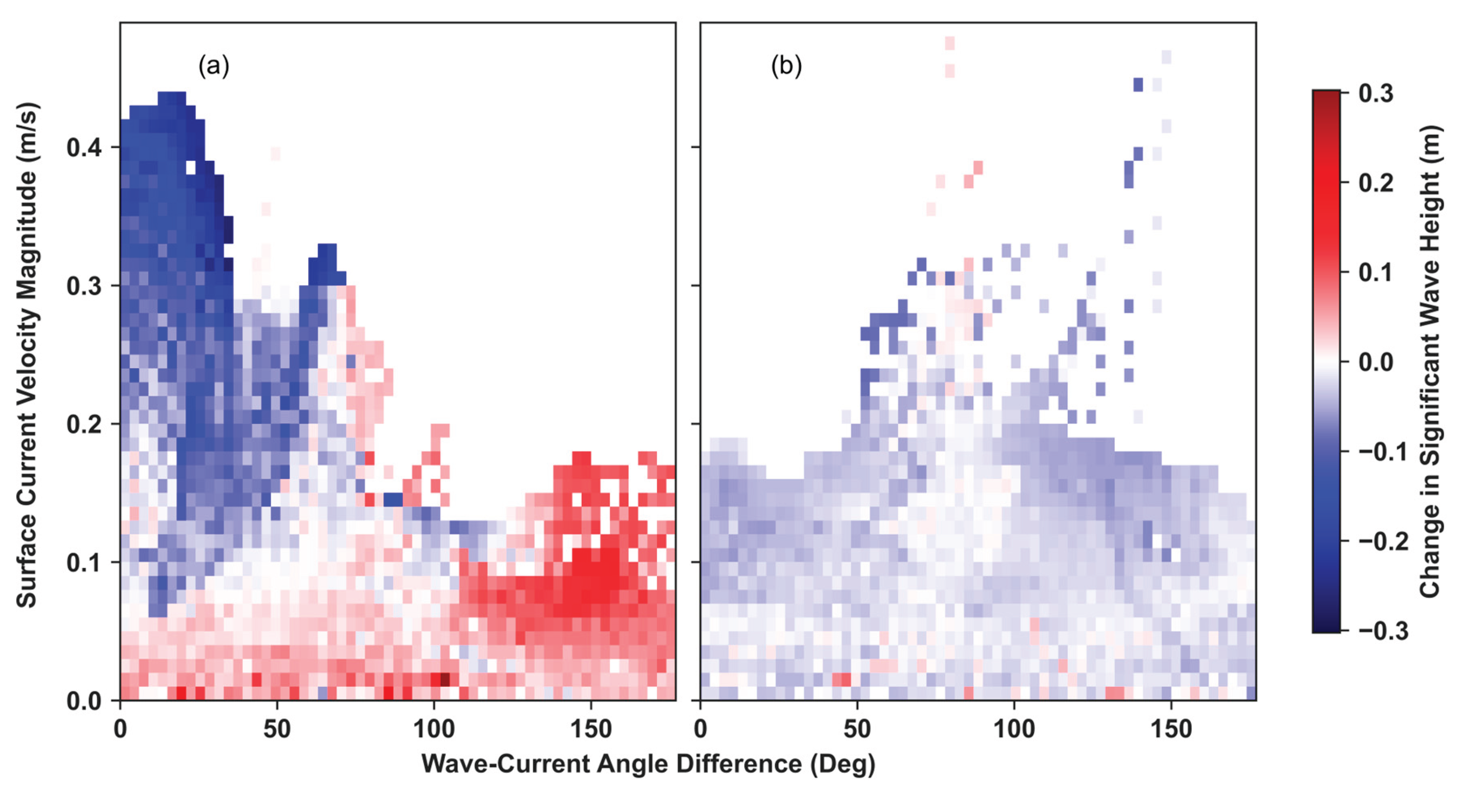
Table 1.
Model cases incorporating the various ST6 physics formulas.
| ST6 Physics | SSWELL | |
| Case 1 | GEN3 ST6 4.7E-7 6.6E-6 4.0 4.0 UP HWANG VECTAU U10PROXY 28.0 AGROW | ARDHUIN 1.2 |
| Case 2 | GEN3 ST6 4.7E-7 6.6E-6 4.0 4.0 UP FAN VECTAU U10PROXY 28.0 AGROW | ARDHUIN 1.2 |
| Case 3 | GEN3 ST6 2.8E-6 3.5E-5 4.0 4.0 UP HWANG VECTAU U10PROXY 32.0 AGROW | ARDHUIN 1.2 |
| Case 4 | GEN3 ST6 2.8E-6 3.5E-5 4.0 4.0 UP HWANG VECTAU U10PROXY 32.0 DEBIAS 0.89 AGROW | ARDHUIN 1.2 |
| Case 5 | GEN3 ST6 6.5E-6 8.5E-5 4.0 4.0 UP HWANG VECTAU U10PROXY 35.0 AGROW | ARDHUIN 1.2 |
| Case 6 | GEN3 ST6 4.7E-7 6.6E-6 4.0 4.0 UP HWANG VECTAU U10PROXY 28.0 AGROW | ZIEGER 0.00025 |
| Case 7 | GEN3 ST6 4.7E-7 6.6E-6 4.0 4.0 UP FAN VECTAU U10PROXY 28.0 AGROW | ZIEGER 0.00025 |
Table 2.
Names of buoys and their locations and depth for model calibration and validation.
| Buoy | Location | Depth |
| Faro Ocean | 36.398°N, 8.068°W | 1334 m |
| Cadiz | 36.490°N, 6.960°W | 450 m |
| Sines | 37.675°N, 9.725°W | 1768 m |
| Faro Coast | 36.905°N, 7.898°W | 90 m |
| Armona | 37.011°N, 7.741°W | 21 m |
Table 3.
Model runs with various hydrodynamic forcing from SOMA.
| Run | Hydrodynamic Input |
| 1 | No Hydrodynamic Input |
| 2 | SOMA Water Level Only |
| 3 | SOMA Surface Currents and Water Level |
| 4 | SOMA Currents (10 m Depth-Averaged Velocity) and Water Level |
| 5 | SOMA Currents (20 m Depth-Averaged Velocity) and Water Level |
| 6 | SOMA Currents (Full Water Column Depth-Averaged Velocity) and Water Level |
Table 4.
Simulation timeframes used for SWAN calibration, validation, and to test hydrodynamic forcing in different wave conditions.
Table 4.
Simulation timeframes used for SWAN calibration, validation, and to test hydrodynamic forcing in different wave conditions.
| Experiment | Timeframe | Dominant Wave Direction | Model Test |
| 1 | 2024-02-01 - 2024-02-29 | Westerly | Standalone SWAN calibration |
| 2 | 2023-11-01 - 2023-11-30 | Westerly | Standalone SWAN validation |
| 3 | 2023-10-21 - 2023-11-07 | Westerly | Hydrodynamic forcing |
| 4 | 2023-02-08 - 2023-02-22 | Easterly | Hydrodynamic forcing |
| 5 | 2023-04-17 - 2023-04-23 | Easterly | Hydrodynamic forcing (shallow waters) |
Table 5.
Error metrics of significant wave height comparing model results of each calibration setting with buoy observations. Values in bold indicate the lowest (RMSE or BIAS) or highest (MSS or R) among all cases.
Table 5.
Error metrics of significant wave height comparing model results of each calibration setting with buoy observations. Values in bold indicate the lowest (RMSE or BIAS) or highest (MSS or R) among all cases.
| Faro Ocean Buoy | Cadiz Buoy | Sines Buoy | ||||||||||
| RMSE (m) | BIAS (m) | MSS | R | RMSE (m) | BIAS (m) | MSS | R | RMSE (m) | BIAS (m) | MSS | R | |
| Case 1 | 0.368 | -0.014 | 0.962 | 0.927 | 0.368 | 0.131 | 0.958 | 0.929 | 0.402 | 0.008 | 0.979 | 0.959 |
| Case 2 | 0.379 | -0.067 | 0.959 | 0.924 | 0.361 | 0.072 | 0.958 | 0.922 | 0.394 | -0.032 | 0.980 | 0.961 |
| Case 3 | 0.369 | 0.011 | 0.962 | 0.927 | 0.381 | 0.151 | 0.956 | 0.928 | 0.404 | 0.018 | 0.979 | 0.959 |
| Case 4 | 0.370 | -0.035 | 0.961 | 0.926 | 0.365 | 0.102 | 0.958 | 0.925 | 0.395 | -0.014 | 0.980 | 0.960 |
| Case 5 | 0.375 | 0.036 | 0.961 | 0.925 | 0.396 | 0.172 | 0.953 | 0.926 | 0.409 | 0.030 | 0.979 | 0.958 |
| Case 6 | 0.366 | -0.001 | 0.963 | 0.928 | 0.374 | 0.138 | 0.958 | 0.929 | 0.404 | 0.021 | 0.979 | 0.959 |
| Case 7 | 0.374 | -0.056 | 0.960 | 0.925 | 0.363 | 0.078 | 0.958 | 0.922 | 0.394 | -0.020 | 0.980 | 0.961 |
Table 6.
Error metrics of Hs, mdir, and Tp between modeled results and observations during the validation period.
Table 6.
Error metrics of Hs, mdir, and Tp between modeled results and observations during the validation period.
| Significant Wave Height (m) | ||||
| RMSE (m) | BIAS (m) | MSS | R | |
| Faro Oceanic Buoy | 0.400 | 0.173 | 0.942 | 0.921 |
| Faro Coast Buoy | 0.156 | -0.016 | 0.973 | 0.951 |
| Cadiz Buoy | 0.407 | 0.255 | 0.900 | 0.914 |
| Sines Buoy | 0.335 | 0.016 | 0.989 | 0.983 |
| Mean Wave Direction (deg) | ||||
| RMSE (deg) | BIAS (deg) | MSS | R | |
| Faro Oceanic Buoy | 20.099 | -6.792 | 0.957 | 0.866 |
| Faro Coast Buoy | N/A | N/A | N/A | N/A |
| Cadiz Buoy | 21.848 | -4.131 | 0.969 | 0.856 |
| Sines Buoy | 8.065 | -0.088 | 0.985 | 0.922 |
| Peak Period (s) | ||||
| RMSE (s) | BIAS (s) | MSS | R | |
| Faro Oceanic Buoy | 3.127 | 1.101 | 0.757 | 0.607 |
| Faro Coast Buoy | 2.878 | 0.559 | 0.806 | 0.670 |
| Cadiz Buoy | 3.522 | 1.546 | 0.760 | 0.625 |
| Sines Buoy | 1.554 | -0.093 | 0.900 | 0.813 |
Table 7.
Error metrics of significant wave height for each model run that implemented the various hydrodynamic forcing for the simulation with westerly waves.
Table 7.
Error metrics of significant wave height for each model run that implemented the various hydrodynamic forcing for the simulation with westerly waves.
| 2023-10-21 12:00:00 - 2023-11-07 12:00:00 – WESTERLY WAVES | ||||||||||||||||
| Faro Oceanic Buoy | Faro Coast Buoy | Cadiz Buoy | Sines Buoy | |||||||||||||
| RUN ID | RMSE (m) | BIAS (m) | MSS | R | RMSE (m) | BIAS (m) | MSS | R | RMSE (m) | BIAS (m) | MSS | R | RMSE (m) | BIAS (m) | MSS | R |
| 1 | 0.526 | 0.407 | 0.905 | 0.926 | 0.246 | -0.025 | 0.957 | 0.933 | 0.594 | 0.502 | 0.862 | 0.922 | 0.427 | -0.112 | 0.979 | 0.966 |
| 2 | 0.525 | 0.407 | 0.905 | 0.926 | 0.242 | -0.034 | 0.958 | 0.933 | 0.593 | 0.501 | 0.862 | 0.921 | 0.421 | -0.111 | 0.980 | 0.967 |
| 3 | 0.472 | 0.356 | 0.920 | 0.931 | 0.256 | 0.058 | 0.952 | 0.923 | 0.430 | 0.323 | 0.919 | 0.933 | 0.398 | -0.048 | 0.982 | 0.967 |
| 4 | 0.474 | 0.358 | 0.919 | 0.931 | 0.258 | 0.065 | 0.951 | 0.924 | 0.436 | 0.330 | 0.918 | 0.934 | 0.402 | -0.047 | 0.982 | 0.967 |
| 5 | 0.475 | 0.360 | 0.919 | 0.931 | 0.258 | 0.064 | 0.951 | 0.925 | 0.439 | 0.334 | 0.917 | 0.934 | 0.402 | -0.048 | 0.982 | 0.967 |
| 6 | 0.569 | 0.455 | 0.892 | 0.924 | 0.252 | 0.005 | 0.956 | 0.934 | 0.580 | 0.485 | 0.868 | 0.922 | 0.398 | -0.026 | 0.982 | 0.968 |
| CMEMS MODEL | 0.365 | 0.125 | 0.940 | 0.902 | 0.186 | 0.001 | 0.966 | 0.943 | 0.265 | 0.104 | 0.959 | 0.939 | 0.391 | -0.165 | 0.983 | 0.975 |
Table 8.
Error metrics of significant wave height for each model run that implemented the various hydrodynamic forcing for the simulation with easterly waves.
Table 8.
Error metrics of significant wave height for each model run that implemented the various hydrodynamic forcing for the simulation with easterly waves.
| 2023-02-08 12:00:00 - 2023-02-22 12:00:00 – EASTERLY WAVES | ||||||||||||
| Faro Oceanic Buoy | Faro Coast Buoy | Sines Buoy | ||||||||||
| RUN ID | RMSE (m) | BIAS (m) | MSS | R | RMSE (m) | BIAS (m) | MSS | R | RMSE (m) | BIAS (m) | MSS | R |
| 1 | 0.338 | -0.205 | 0.972 | 0.964 | 0.305 | -0.161 | 0.972 | 0.964 | 0.373 | 0.203 | 0.890 | 0.874 |
| 2 | 0.343 | -0.221 | 0.971 | 0.966 | 0.326 | -0.217 | 0.967 | 0.964 | 0.364 | 0.184 | 0.894 | 0.872 |
| 3 | 0.325 | -0.210 | 0.974 | 0.970 | 0.290 | -0.143 | 0.974 | 0.962 | 0.352 | 0.170 | 0.900 | 0.874 |
| 4 | 0.318 | -0.196 | 0.975 | 0.970 | 0.288 | -0.133 | 0.974 | 0.962 | 0.360 | 0.182 | 0.896 | 0.874 |
| 5 | 0.318 | -0.195 | 0.975 | 0.970 | 0.289 | -0.133 | 0.974 | 0.962 | 0.360 | 0.183 | 0.896 | 0.874 |
| 6 | 0.411 | -0.302 | 0.958 | 0.961 | 0.297 | -0.156 | 0.972 | 0.963 | 0.367 | 0.192 | 0.893 | 0.874 |
| CMEMS MODEL | 0.427 | -0.312 | 0.947 | 0.968 | 0.379 | -0.293 | 0.945 | 0.970 | 0.334 | 0.209 | 0.906 | 0.899 |
Table 9.
Error metrics of significant wave height for the simulation 2023-04-17 – 2023-04-23.
| Level 1 SIMULATION 2023-04-17T12:00 - 2023-04-23T12:00 | ||||||||||||
| Armona Buoy | Faro Coast Buoy | Cadiz Buoy | ||||||||||
| Run | RMSE (m) | BIAS (m) | MSS | R | RMSE (m) | BIAS (m) | MSS | R | RMSE (m) | BIAS (m) | MSS | R |
| 1 | 0.124 | -0.039 | 0.973 | 0.957 | 0.148 | -0.083 | 0.944 | 0.925 | 0.137 | 0.035 | 0.972 | 0.957 |
| 2 | 0.125 | -0.023 | 0.972 | 0.954 | 0.144 | -0.076 | 0.947 | 0.925 | 0.137 | 0.035 | 0.972 | 0.957 |
| 3 | 0.123 | -0.015 | 0.972 | 0.955 | 0.134 | -0.068 | 0.952 | 0.929 | 0.129 | 0.015 | 0.976 | 0.958 |
| 4 | 0.126 | -0.015 | 0.971 | 0.954 | 0.133 | -0.065 | 0.952 | 0.928 | 0.130 | 0.022 | 0.976 | 0.957 |
| 5 | 0.125 | -0.016 | 0.971 | 0.954 | 0.134 | -0.066 | 0.952 | 0.928 | 0.130 | 0.023 | 0.976 | 0.957 |
| 6 | 0.124 | -0.019 | 0.972 | 0.954 | 0.135 | -0.079 | 0.952 | 0.938 | 0.141 | 0.051 | 0.971 | 0.956 |
| CMEMS MODEL | 0.153 | -0.010 | 0.950 | 0.945 | 0.163 | -0.059 | 0.898 | 0.899 | 0.217 | -0.151 | 0.923 | 0.955 |
Disclaimer/Publisher’s Note: The statements, opinions and data contained in all publications are solely those of the individual author(s) and contributor(s) and not of MDPI and/or the editor(s). MDPI and/or the editor(s) disclaim responsibility for any injury to people or property resulting from any ideas, methods, instructions or products referred to in the content. |
© 2025 by the authors. Licensee MDPI, Basel, Switzerland. This article is an open access article distributed under the terms and conditions of the Creative Commons Attribution (CC BY) license (http://creativecommons.org/licenses/by/4.0/).
Copyright: This open access article is published under a Creative Commons CC BY 4.0 license, which permit the free download, distribution, and reuse, provided that the author and preprint are cited in any reuse.


