Submitted:
11 October 2025
Posted:
13 October 2025
You are already at the latest version
Abstract
Studies of the environmental footprint of large language model (LLM) inference often disagree because they mix incompatible system boundaries, ignore latency and throughput service level objectives (SLOs), and optimize carbon without accounting for water. We present a provider-agnostic framework that unifies scope-transparent measurement with time-resolved, bi-objective orchestration under realistic SLOs. Measurement follows production practice and reports daily medians at a comprehensive serving boundary that includes active accelerators, host CPU/DRAM, provisioned idle, and facility overhead via PUE. Consumptive water is computed as site plus source. Carbon is location-based (LB) by default with a market-based (MB) sensitivity.
Optimization is cast as a mixed‑integer linear program, solved over 288 five‑minute windows per day. For each prompt profile, the solver selects region, batch size, and phase‑aware hardware for prefill and decode while enforcing p95 Time To First Token/Time Per Output Token (TTFT/TPOT) and capacity constraints. Because grid carbon intensity (CIF) and electricity water intensity (EWIF) are only weakly correlated, the policy is dual‑objective by design and balances carbon and water explicitly.
Applied to four representative models using public per‑prompt energy tables and per‑region multipliers, a single SLO‑aware policy reduces comprehensive‑boundary medians by 57-59% for energy, 59-60% for consumptive water, and 78-80% for LB CO_2, with SLOs met in every window. For a day with 500M queries on GPT‑4o, median‑scaled totals drop from 0.344 to 0.145~GWh, 1.196 to 0.490~ML, and 121 to 25~tCO_2 (LB). The framework also reproduces the production‑observed accelerator‑only versus comprehensive gap (narrow/comprehensive approx. 0.417), enabling direct translation across studies. Pareto analyses show when routing alone and when joint routing, batching, and token‑length controls deliver concurrent reductions in carbon and water at fixed quality of service. The combination of time‑resolved control, comprehensive accounting, and dual‑objective optimization yields a deployable template for decarbonization and water stewardship in LLM serving.
Keywords:
LLM inference
; carbon-aware routing
; water-aware routing
; geo-distributed datacenters
; SLO
; TTFT
; TPOT
; MILP
; CIF
; EWIF
; PUE
; WUE
1. Introduction
The deployment of large language models on scale has reshaped the sustainability discussion for artificial intelligence [1,2]. Early work focused almost exclusively on the training phase because one-off runs for frontier models were shown to consume on the order of thousands of megawatt-hours, emit hundreds of tons of CO2 equivalent, and use large volumes of cooling water for a single training job [3,4,5]. Those numbers rightly drew attention and motivated research on efficient architectures and carbon-aware training [6,7]. The landscape has since changed. Public adoption has turned inference into a continuous and interactive service that runs every minute of the day. The cumulative footprint of serving billions of queries now dominates the life-cycle of many deployments and can exceed training by a wide margin [5,8]. Several analyzes estimate that inference can account for up to 90% of the lifetime energy and that the annual operating energy of the large-scale service can be tens of times higher than the energy used to train the model [5,9,10]. A single short prompt appears small when measured in watt-hours, yet at hundreds of millions of prompts per day, the aggregate demand reaches utility-scale electricity and meaningful volumes of water [5]. It follows that sustainability efforts that target training alone are no longer sufficient.
Accurate accounting for inference is challenging, and the literature has only recently converged on methods that match production practice [11]. Early estimates combined accelerator nameplate power, theoretical FLOPs, and assumed token lengths, producing per-prompt energies that differed by an order of magnitude because each study chose different utilization factors and boundaries [5,12,13]. Empirical instrumentation is now emerging through industry studies [1]. A key result from this line of work is that narrow measurement—accelerator only—misses material contributors such as host CPU and DRAM, provisioned idle, and facility overhead captured by power usage effectiveness. Google’s recent production study reports medians at a comprehensive serving boundary and shows that accelerator-only accounting can underestimate per-prompt energy by more than a factor of two for the same workload [1]. This boundary choice explains much of the spread in earlier per-prompt claims and makes clear that scope-transparent reporting is a prerequisite for credible comparison and for effective optimization.
Water has been even less visible in model reporting despite its central role in data center operations [3,5,14]. Cooling systems withdraw and consume water on site, and electricity generation for computing carries a significant upstream water intensity [15]. Model cards and environmental summaries often report scope 2 carbon while omitting water entirely [16,17]. The omission matters because the water intensity of electricity and the carbon intensity of the grid vary by region and time, and they are only weakly correlated. A policy that pursues the lowest carbon intensity without regard to water can inadvertently increase total water consumption, for example by shifting the load to nuclear-heavy or hydro-dominated regions where the liters per kilowatt-hour are higher, while the converse can also occur [3,14]. Recent studies document that carbon and water can move in opposite directions, which means sustainability must be treated as a bi-objective problem rather than a single number to be minimized [14].
Any practical solution must also respect the realities of an interactive service [18]. LLM serving is governed by strict service level objectives for responsiveness. Time to first token and time per output token directly shape perceived latency and throughput [17]. Production systems cannot delay user requests to wait for a greener grid, nor can they indiscriminately route traffic to distant regions if that violates latency budgets. The optimization space is therefore bounded by performance constraints and by the capacity of the serving fleet. A sustainability framework that ignores these constraints does not translate into production.
This paper proposes a deployment-aware framework that unifies measurement and control. The approach is provider-agnostic, scope transparent by construction, and explicitly bi-objective in carbon and water. Measurement follows production practice and reports daily medians at a comprehensive serving boundary that includes active accelerators, host CPU and DRAM, provisioned idle, and PUE uplift [1]. Consumptive water is computed as the site plus the source using [3]. Carbon is location based by default with a market-based sensitivity when portfolio factors are disclosed. Optimization casts serving orchestration as a mixed-integer linear program solved over 288 five-minute windows per day. For each prompt profile the solver chooses region, batch size, and a phase-aware hardware assignment that separates prefill and decode. The formulation enforces constraints on time to first token and time per output token, augmented by a per-region network term. Capacity constraints derive from measured tokens-per-second tables. Token-length directives are modeled as controllable reductions in decode work.
Our contributions are fourfold. First, we provide a full-stack, scope-transparent accounting for inference that reproduces the production gap between accelerator-only and comprehensive boundaries and supplies a defensible translation between the two, with a narrow-to-comprehensive median ratio of about 0.417 for the workloads we study [1]. Second, we formulate a time-resolved, bi-objective optimizer that co-minimizes location-based carbon and consumptive water under explicit SLOs and fleet capacity. Third, we demonstrate the framework on four representative models using public per-prompt energy tables and provider PUE, WUE, and carbon factors, and we show that a single SLO-aware policy reduces comprehensive medians by roughly 57–59% for energy, 59–60% for water, and 78–80% for location-based CO2 while meeting latency and throughput targets in every window. Fourth, we analyze routing-only and joint routing+batch+token frontiers to make the carbon–water geometry explicit, which tells operators when improvements move both metrics together and when trade-offs must be managed.
The remainder of the paper is organized as follows. Section 2 surveys the literature and motivates comprehensive boundaries, water-aware metrics, and SLO-respecting orchestration. Section 3 details the methodology, including the functional unit, scope definitions, impact accounting, time resolution, decision variables, constraints, and parameterization. Section 4 presents the results, reporting comprehensive-boundary medians and daily totals, scope reconciliation between accelerator-only and comprehensive views, and carbon–water movement at fixed quality of service with routing, batch, token, and phase-split analyses. Section 5 discusses implications, deployment guidance, and limitations, and outlines directions for future work. Section 6 concludes the paper.
2. Optimizing the Environmental Footprint of LLM Inference: A Literature Review
2.1. From Training to Inference: Why the Burden Has Shifted
Early work on AI sustainability emphasized training, where single jobs for frontier models consumed thousands of MWh and emitted hundreds of tons of CO2e while using significant cooling water [3,4,5,6,7]. As generative systems moved into daily use, the continuous nature of serving billions of prompts has become the dominant lifecycle driver for many deployments [5,8,9,10,19,20,21]. Per-request impacts that seem small in isolation compound at scale: a single ChatGPT-style prompt has been estimated at several grams CO2e, far above a web search [22], and daily volumes in the hundreds of millions translate to utility-scale electricity and meaningful water withdrawals [5]. These observations motivate methods that measure inference accurately and optimize it under interactive quality constraints.
2.2. Full Stack per Prompt Accounting: Energy, Carbon, Water, and Embodied Impacts
Production studies recommend a comprehensive serving boundary that includes the active accelerator, host CPU and DRAM, provisioned idle, and facility overhead via PUE [1,23,24]. Under this boundary, “accelerator only” views can undercount by more than a factor of two. The Google study reports a narrow-to-comprehensive median ratio near for similar workloads [1]. Carbon per prompt should be reported both location based (grid average) and, when portfolios are disclosed, market based [25], and it should include amortized embodied impacts from hardware manufacturing where possible [26,27,28]. Water deserves first-class treatment: consumptive site cooling scaled by PUE plus off-site electricity–water intensity (EWIF) yields a scope-consistent measure of liters per kWh that varies widely by region and generation mix [3,29,30,31,32,33]. Because carbon intensity (CIF) and EWIF are only weakly correlated, any realistic framework should measure both and co-optimize them [3,14].
2.3. Measurement Boundaries: Why Scope Transparency Matters
Inconsistent boundaries explain much of the order-of-magnitude spread in earlier per-prompt estimates. Studies that measured only chip power (sometimes at unrealistic utilization) omitted host, idle, and cooling overheads and thus overstated efficiency [5,34,35]. Converging practice now recommends a comprehensive inference boundary under operator control, with explicit exclusions outside that boundary (e.g., end user devices or wide-area network transit) and with scope-transparent reporting so results are comparable across systems [1,24]. The ≈0.417 narrow-to-comprehensive ratio provides a defensible translation when only accelerator-level numbers are available and site factors and mixes are held constant [1]. Our methods section adopts this convention and reports daily medians to handle skewed mixes.
2.4. Real-Time Orchestration: Carbon- and Water-Aware Routing Under SLOs
With consistent measurement in place, the next step is optimization. Carbon-aware request routing has been shown to cut serving emissions substantially without violating latency when traffic is steered to cleaner grids in space and time [10,36,37,38,39]. Projections suggest even larger reductions as grids decarbonize and capacity headroom grows [10]. Emerging frameworks treat scheduling as a multi-objective problem, co-optimizing carbon, water, and cost while enforcing latency SLOs and site capacity constraints; practical solutions range from MILPs to learning-based controllers [9,40,41,42,43]. Our
2.5. Phase-Aware Hardware Scheduling (Prefill vs. Decode)
Transformer serving has two phases with different bottlenecks. Prefill is parallel and compute-heavy. Decode is sequential and often memory-bound [44,45]. Phase-aware scheduling assigns prefill and decode to different hardware or configurations to improve both responsiveness and efficiency [1,46,47,48]. Speculative decoding and KV-cache reuse further reduce decode work [49,50]. Our formulation exposes prefill and decode decisions and allows second-life hardware to serve decode when SLOs permit [22,51].
2.6. Semantic-Level Interventions
Beyond systems levers, generation can be made more efficient with semantic directives that reduce unnecessary output length or avoid high-compute behaviors while preserving usefulness. SPROUT exemplifies this approach, reporting large carbon savings with minimal impact on quality by selectively applying concise directives [52]. Related work on eco-adaptive services explores small, user-acceptable adjustments during high-carbon periods to achieve large operational reductions [21]. These methods complement, rather than replace, hardware and orchestration optimizations.
2.7. Lifecycle and Circular Economy Strategies
Holistic sustainability includes upstream manufacturing and end of life. Hardware production for AI accelerators is energy- and material-intensive; embodied emissions can dominate in low-carbon operational settings [53,54]. Scenario analyses warn of rapid growth in AI-related e-waste, and point to device life extension, refurbishment, parts harvesting, and improved recycling as the most effective mitigations [55]. Second-life deployment and modular upgrades align with extended producer responsibility and reduce both embodied and disposal impacts [1,22,55].
2.8. Toward a Unified, Deployment-Aware Framework
Across the literature a consensus is emerging: inference now dominates impacts [5,8,9,10,19,20,21]; scope-transparent, full-stack per-prompt accounting is essential [1,23,24,25]; optimization must be bi-objective in carbon and water and must observe latency SLOs [3,9,10,14,36,37,38,39]; and lifecycle thinking is required to avoid shifting costs upstream or downstream [22,53,54,55]. Persistent gaps remain—especially inconsistent boundaries and limited treatment of water. The present work addresses these gaps by (i) adopting comprehensive, production-style measurement with explicit narrow↔comprehensive translation; (ii) integrating EWIF alongside CIF so water is optimized jointly with carbon; (iii) enforcing TTFT/TPOT and capacity constraints so results are deployable; and (iv) exposing phase-aware and semantic levers that reduce watt-hours per prompt while maintaining interactive quality. Together, these elements provide a practical path for operators to measure, compare, and materially lower the environmental footprint of LLM serving.
3. Methodology
The aim of the methodology is to turn non-comparable measurements of LLM inference into one portable, auditable workflow that: (i) reports apples-to-apples per-prompt medians under a comprehensive serving boundary consistent with production practice and, when needed for comparison, under a narrower accelerator-only boundary; (ii) enforces real SLOs through explicit capacity and latency constraints derived from public tokens-per-second and latency quantiles; and (iii) co-optimizes energy, location-based (LB) greenhouse-gas emissions, consumptive water, and amortized embodied impacts through a mixed-integer linear program (MILP). The comprehensive boundary follows the decomposition implemented in a recent first-party production study for Gemini Apps, which measures the median text prompt at Wh (comprehensive) with an accelerator-only median of Wh when active accelerator, host CPU/DRAM, provisioned idle, and facility overhead (PUE) are aggregated [1]. These medians imply an uplift of due purely to boundary choice (comprehensive vs. accelerator-only). We adopt that full-stack paradigm for comparability and to avoid systematic undercounting identified by the production study [1].
3.1. Functional Unit and System Boundaries
The functional unit is one served prompt. We compute energy per prompt in watt-hours at two nested system boundaries so that our results are comparable to both “narrow” and “comprehensive” studies [1]. Accelerator-only boundary counts only the active accelerator energy directly attributable to the prompt. Comprehensive serving boundary adds host CPU/DRAM, provisioned idle capacity, and facility overhead captured by PUE. We adopt this boundary as our default because it aligns with production telemetry and produces apples-to-apples medians across models and regions [1].
Let denote accelerator-only energy per prompt (i.e., the GPU/TPU compute energy for the prefill and decode phases). It excludes host CPU/DRAM energy, provisioned-but-idle energy, and any facility overhead captured by ; the IT energy per prompt (accelerators + host CPU/DRAM + provisioned idle); and the per-prompt energy used on non-accelerator hardware that is part of serving the request: host CPUs, DRAM, NICs, disks on the inference nodes (and sometimes service sidecars); the ratio of total IT-side energy (accelerator active + host + idle) to the accelerator’s active energy:
To be numerically consistent with the reported medians ( Wh and Wh [1]), we set and thus obtain When host/idle shares are undisclosed, we use this aggregated rather than point estimates for and .
We define: the facility energy per prompt (what the whole data center expends to deliver the prompt), with we have Wh per text prompt. This matches the comprehensive median found in [1] and implies a uplift over the accelerator-only median ( Wh) for the same workload.The overhead energy is exactly the extra above IT:
3.2. Impact Accounting
We compute operational emissions using the location-based (LB) approach recommended for data-center Scope-2 reporting [1]. The facility energy associated with serving one prompt, (kWh prompt−1), is multiplied with location-based grid carbon intensity for region r, (kgCO2kWh−1). This yields the LB, per-prompt operational emissions:
LB attributes emissions to the electricity actually drawn from the local grid at the point of consumption and is the basis for statistically comparable across operators and regions, aligning with routing-aware decisions, and avoids year-to-year swings caused by portfolio accounting. For the sensitivity we also compute the provider’s prior-year portfolio emission factor (kgCO2e kWh−1) [25]. MB, when disclosed, can be reported as a sensitivity and makes results operationally interpretable while retaining comparability. We use LB as the objective default and MB as a sensitivity. Operational emissions are reported in g CO2 (LB); g CO2e is reserved for MB factors and embodied/lifecycle terms.
For water, we follow the scope-consistent “site + source” rule advocated in the AI water-footprint literature [3]. Consumptive site water (cooling, at the facility) is proportional to facility energy via the site Water Usage Effectiveness (LkWh−1) while source water accounts for the electricity-generation water intensity of the regional grid via the Electricity-Water Intensity Factor (LkWh−1), separating site water (cooling; WUE Category 2) from source water associated with electricity generation (EWIF), as recommended in the water-footprint literature [3]. Using for the electrical work of the IT load, the per-prompt consumptive water is:
This form makes explicit that site water scales with the facility energy (hence the multiplier), while source water scales with the electricity used to power the IT equipment and is governed by the grid mix. Analysis emphasizes both the need to include scope-2 water and the empirical weak correlation between carbon and water intensities [3], motivating dual-metric reporting and optimization. The macro background on facility-level and levels across the U.S. fleet is taken from the 2024 U.S. Data Center Energy Usage Report, which shows hyperscale-weighted averages below ∼1.4 and site around – LkWh−1 in 2023 (with a likely rise as liquid cooling penetrates), giving realistic bounds for sensitivity tests [56].
We summarize per-prompt footprints (Wh, mL, gCO2e) as daily medians by profile and season, mirroring the production study’s choice of medians as the right statistic for skewed mixes; that study reports comprehensive-boundary medians near Wh, gCO2e, and mL for the median text prompt and documents the uplift from accelerator-only to comprehensive accounting. Our framework reproduces this uplift when we apply and to chip-only numbers, providing scope-transparent comparability [1].
We include embodied impacts and e-waste on a serving-time basis. For accelerator class h with embodied carbon (kgCO2e board−1), board mass (g), and assumed service lifetime (days), we compute daily rates (kgCO2e day−1) and (g day−1). When a class is activated (binary variable in the solver), we allocate its daily embodied rates to the prompts it serves that day, adding an amortized per-prompt embodied term that brings hardware lifecycle into scope. This aligns with the lifecycle scope of the production study [1,22].
3.3. Time Resolution, Traffic Mix and SLOs
We partition a day into decision windows of five minutes each with budget s. Demand is described by three prompt profiles with token pairs equal to , , and . Unless noted, arrivals total M prompts per day with a mix. Windowed arrivals are either provided or constructed from , the mix , and diurnal weights as .
The router chooses non-negative integer assignments by region r, hardware class h, batch size b, phase , and directive . Prefill and decode are two legs of the same request, so conservation holds per window and profile as in Equation (6). Capacity in a five-minute window is enforced with quantile throughputs , which bound the total tokens processed per provisioned node at batch b; Equation (7) applies this limit with the window budget .
Latency SLOs use profile-specific targets. We work with the published per-hardware, per-batch quantiles for TTFT and TPOT and the associated rows. The formulation imposes the tail-latency guard of Equation (8) at and uses the same throughputs in the capacity constraint so feasibility reflects the stochastic nature of serving. Unless otherwise stated, reported summaries are daily medians by profile and a mix of those medians, which is consistent with production practice for skewed mixes and utilization patterns [1].
3.4. Decision Variables, objEctive and Constraints
The decision variables are the assignment of prompts in each window (non-negative integers), binary activation variables for hardware classes at a site, the chosen batch size b from a small discrete set per hardware, binary indicators that switch on embodied amortization when a hardware class is used and : the number of replicas provisioned at in window t. Parameters include the per-site replica cap and the big-M constants and used in activation/feasibility linkages.
Each prompt of profile p consists of input tokens in the prefill phase and output tokens in the decode phase. Decode tokens are scaled by the directive factor , which can take values such as , , or depending on whether the output is shortened. The number of tokens served by a routed block is therefore given by:
Throughput is modeled as , the number of tokens per second at quantile q for hardware class h under batch size b. Latency SLOs are profile-specific constants , for example s for “short” prompts.
We aggregate to daily medians per profile and mix by 70/25/5. The objective is a weighted-sum scalarization with non-negative policy weights:
where minimization is over the decision variables . The weights are chosen by the operator/policy. Equation (5) mirrors multi-impact scoring used in recent infrastructure-aware benchmarking (energy, water, carbon) while adding embodied and e-waste terms for life-cycle completeness [5].
Prefill and decode are two legs of the same request; counts must match and meet demand. The first constraint to satisfy this, a linear one, is:
As we cannot push more tokens through a node in five minutes than the node can handle at the selected batch and the specified throughput quantile, we impose the second constraint, capacity using quantile throughput from the benchmark (per hardware/batch):
where s is the five-minute budget and unless noted. We enforce and for all , and gate assignments by for all .
The third constraint is tail latency controlled by bounding the response time per profile to its SLO :
To evaluate the objective, we expand each impact term at the level of a single routing assignment . We first compute accelerator-only energy (Wh), after which the solver chooses an assignment count. In each 5-minute window t:
with energy per output token in decode:
where is the accelerator-only average power (W).
Before the first token appears, the system spends seconds on prefill; spreading that energy over the input tokens for profile p makes the prefill term linear and comparable:
We then lift to IT energy with the production-observed host+idle scaler (cf. Equation (1)), and to facility (comprehensive) energy via the site’s :
Consumptive water is obtained by applying the site-level cooling term and source-site electricity water to IT energy:
Operational emissions use facility energy times either the provided market-based factor or the location-based grid factor; with LB as default:
Finally, the embodied CO2 and e-waste are amortized as daily charges that activate once per hardware class used:
Summing Equations (9)–(16) over all assignments in a window yields the window-level that enter the objective in (5); summing over t and taking daily medians produces the reported statistics, with LB as default and MB as sensitivity [1,3,25,56].
| Algorithm 1 -Scale (daily-coupled MILP; p95 SLOs, replicas, daily binaries) |
|
| Algorithm 2 Aggregation and scope-transparent reporting (post-solve) |
|
3.5. Parameterization from Public Sources
We adopt the comprehensive serving boundary by default: active accelerators together with host CPU/DRAM and provisioned idle, lifted to facility energy by the site PUE in Equations (12)–(13). When only accelerator-only measurements are disclosed, we translate to the comprehensive boundary with a host+idle lift and PUE, or when shares are undisclosed, by using the production-observed narrow→comprehensive median ratio for comparable workloads [1]. Reporting uses daily medians to mirror production practice and to keep results comparable across models and regions [1].
Baseline per-prompt energy and throughput/latency quantiles by model and profile are taken from the cross-model API benchmark [5]. We ingest watt-hours per prompt together with the p-quantile tokens-per-second and latency rows, for example p95 TTFT, TPS, and TPOT. These quantiles parameterize the capacity and tail-latency constraints in Equations (7)–(8). As an illustration, the table for GPT-4o lists a short-profile energy near Wh and provides site multipliers; we keep the published provider/region mapping [5].
Per-token coefficients for prefill and decode follow the device-level accelerator-only power models used in Equations (10)–(11). The average accelerator power is taken per hardware class and batch. We lift accelerator-only energy to IT with the host+idle scaler in Equation (12) and then to facility with the site PUE in Equation (13), consistent with the comprehensive boundary in [1].
Consumptive water is computed with the scope-consistent site+source formulation in Equation (14). The site component scales with facility energy via . The source component scales with IT energy via the regional electricity–water intensity factor . Priors and bounds for site WUE come from the LBNL synthesis and AI water-footprint guidance [3,56]. Electricity–water intensity values follow the scope-2 definition in [3] and are applied as annual, location-based factors when hourly mixes are unavailable.
Operational emissions are location-based by default using regional CIF with facility energy in Equation (15). We also provide a market-based sensitivity by substituting the provider’s prior-year portfolio factor when disclosed [1,25]. Units are reported in the native form for each metric.
For the phase-aware variant, we use accelerator-only per-token energy curves that separate compute-bound prefill from memory-bound decode across relevant batches. This enables assignments that reduce Wh per prompt while respecting p95 SLOs [22]. Embodied carbon per board, board mass, and lifetimes are taken from serving and lifecycle assessments [16,53] and are amortized once per day when a hardware class is activated, as in Equation (16).
Reference ranges for site factors follow [56]. Hyperscale PUE trends to roughly –. Site WUE is around – L kWh−1 in 2023 with a likely rise as liquid cooling penetrates. Scenario sweeps therefore use around a regional PUE baseline and around site WUE. When we construct hydro-like or nuclear-like sites for Pareto illustrations, CIF and electricity–water intensity are kept within documented ranges and flagged as replaceable medians when provider rows are disclosed [3,56].
All numerical inputs—per-model Wh per prompt, p95 TTFT/TPS/TPOT by batch, site rows with PUE, site WUE, electricity–water intensity, and location-based carbon intensity, and embodiment parameters—are taken from peer-reviewed or provider-authored sources [1,3,5,56]. We package them into machine-readable tables so figures and results regenerate one-for-one when providers update disclosures. When deployment caps are known, we set to the maximum provisionable replicas for class h at region r and batch b. Otherwise is a large operator-chosen bound.
Because grid carbon intensity and electricity–water intensity can be weakly correlated at fine time scales, improving one can worsen the other [3]. This motivates the bi-objective treatment and the routing-only and joint routing+batch+token analyses that make the trade-off geometry explicit under p95 SLOs.
4. Results
We simulate a single 24 hour production day split into 288 five-minute decision windows and a fixed demand of 500 million prompts with a short/medium/long mix. Short, medium, and long profiles use token pairs , , and , respectively. In every window the Scale optimizer chooses, for each profile, the region, the batch size, and the phase-specific hardware (prefill vs. decode) to minimize an equal-weighted sum of energy, consumptive water, and location-based CO2 subject to explicit SLOs and the capacity and conservation constraints. Capacity is enforced with per-hardware, per-batch tokens-per-second quantiles, and latency feasibility uses time-to-first-token and time-per-output-token; the short prompt target is s. Window outputs are aggregated to daily medians per profile and then mixed by to obtain per-model medians. By default we report the comprehensive serving boundary—active accelerator + host CPU/DRAM + provisioned idle—lifted to facility energy by the site’s . Consumptive water is computed with the scope-consistent site+source rule, ; CO2 is location-based using , with a market-based sensitivity when prior-year portfolio factors are available. For reconciliation with chip-only studies we also compute an accelerator-only subset and translate between scopes using the empirically observed narrow/comprehensive median ratio of (approximately uplift; e.g., Wh accelerator-only vs. Wh comprehensive at the median) [1]. Regional multipliers (, , , ) and the throughput/latency quantiles that bind the SLOs come from the cross-model public benchmark; a phase-aware variant uses device-level per-token energy curves for prefill/decode and includes embodied-carbon amortization when a hardware class is activated during the day [5]. Two policies are evaluated under identical demand and site multipliers. The baseline fixes batch , uses the home region only, applies no token directive, and does not split phases. The Scale optimized policy right-sizes batch over the day, applies a concise token directive when SLO-safe, routes across sites in response to CIF and , assigns prefill and decode to different hardware when that lowers Wh/prompt, and amortizes embodied impacts; the contrast between these policies isolates the value of orchestration at a fixed model and boundary.
4.1. Comprehensive Boundary Medians and Daily Totals
Table 1 reports per-prompt median-scaled total and associated daily totals for energy, water (consumptive, site+source), and location-based CO2 for four representative models. The Optimized rows correspond to the Scale loop with all levers active (batch right-sizing, semantic token control, geo-routing, phase-aware assignment, and second-life amortization). Baseline uses the same comprehensive boundary and medians but with batch , no token control, home region only, and no phase split. Across the four evaluated models, the Scale policy delivers large and consistent savings at the comprehensive serving boundary. After aggregating window outputs to daily medians per profile and mixing by , the median energy per prompt falls by 57–, the median consumptive water (site+source) by 59–, and the median location-based CO2 by 78–, all while meeting capacity and latency in every five-minute window. For GPT-4o, the comprehensive baseline is Wh/prompt, mL/prompt, and g CO2/prompt; after optimization the medians become Wh, mL, and g CO2, respectively. At a volume of 500 M queries per day these medians translate to energy dropping GWh, water ML, and LB CO2 t under the same SLA. The other models follow the same pattern, with absolute magnitudes scaling with baseline Wh/prompt (e.g., Claude 3.7 Sonnet shows the largest absolute reductions because its baselines are highest). These gains reflect full-stack serving and scope-consistent water accounting rather than chip-only power, and they arise from the combined effect of batch right-sizing (e.g., off-peak), token-length directives, carbon- and water-aware geo-routing, phase-aware hardware assignment, and second-life amortization. See Figure 1 for a side-by-side visualization of the comprehensive-boundary medians (baseline vs. optimized) for energy, consumptive water, and LB CO2, with lower ‘scope whiskers’ showing accelerator-only values via the observed narrow/comprehensive ratio.
4.2. Scope Reconciliation: Accelerator-Only vs. Comprehensive
A persistent source of disagreement in the literature is the accounting boundary used for inference. To make our results directly comparable to chip-only studies, we compute both scopes for the same traffic, mix, and site multipliers and place them side by side. The empirical narrow/comprehensive median energy ratio in our runs is , reproducing the uplift observed in production telemetry when host CPU/DRAM, provisioned idle, and facility overheads () are included [1]. This factor is not universal—it varies with architecture and fleet management—but when underlying shares are unavailable it provides a defensible translation between scopes. Concretely, if a study reports only accelerator-level energy (Wh prompt−1), the comprehensive median may be approximated by , holding , , , and the prompt mix constant.
Table 2 provides scope translation to reconcile chip-only studies with comprehensive accounting. The numerical proximity between optimized comprehensive and baseline narrow in our run ( of baseline comprehensive in both cases) is coincidental: the former reflects optimization levers and SLOs; the latter reflects boundary accounting shares measured in production. Together with Table 1 (policy effects at the comprehensive boundary), Table 2 furnishes a clear, citable translation layer so that chip-only results can be reconciled with full-stack accounting without ambiguity.
4.3. Carbon–Water Movement at Fixed QoS
Because grid carbon intensity () and electricity-water intensity () are weakly correlated, carbon-optimal routing can be water-suboptimal. Our Scale policy jointly optimizes both metrics. Figure 2 shows each model’s movement from baseline to optimized in the plane. For each model we plot the comprehensive-boundary median at the baseline configuration and the corresponding median under the Scale policy; the two points are connected by an arrow. In every case the arrow points down and to the left, showing that the optimized policy reduces both location-based CO2 and consumptive water while honoring the SLOs. This simultaneous reduction is non-trivial because and are only weakly correlated; a carbon-only router can increase water if it shifts load to a clean but water-intensive region. The Scale objective avoids that pitfall by jointly reducing Wh per prompt—through batch right-sizing, concise token directives, and phase-aware placement—and by routing remaining Wh to regions and hours with favorable and .
The geometry is intuitive. Each site i defines a ray through the origin in the plane whose slope is , with . Moving along a ray changes only energy (Wh) via batching and token control; switching rays changes the water-to-carbon ratio by altering site factors while holding Wh fixed. The optimizer exploits both degrees of freedom: it lowers Wh and, subject to the latency budget, selects rays with more favorable slopes. In a two-region sensitivity where the alternative site is hydro-like with both lower and a lower combined water factor, routing alone becomes a Pareto improvement; the arrow’s down-left direction then reflects a pure siting effect. In other configurations, the arrow still points down-left because energy reductions combine with selective routing to offset sites where low carbon coincides with higher water.
To keep scope visible without obscuring directionality, Figure 2 overlays asymmetric boundary whiskers on both endpoints. The barbed end of each whisker marks the accelerator-only value obtained by multiplying the comprehensive coordinate by on both axes; there is no upper whisker because comprehensive is our defined upper boundary. The tip-to-tail arrows and their whiskered counterparts are nearly parallel and scaled, illustrating that the direction and magnitude of the optimization gain are robust to scope choice: changing scope shifts absolute values by the familiar but does not alter the qualitative improvement.
This figure is diagnostic rather than a full carbon–water Pareto frontier. Constructing that frontier would require multiple MILP runs with different objective weights. At fixed QoS, the comprehensive, SLO-aware policy achieves concurrent reductions in CO2 and water for the evaluated workloads. In the next section we quantify the additional reductions available if small latency relaxations or stronger token-length directives are permitted.
4.4. Routing-Only Carbon–Water Pareto Under SLOs
The previous subsection established that the Scale policy moves every model down and to the left in the plane: batching and token directives reduce watt-hours per prompt, while geo-routing chooses sites whose environmental multipliers further shrink carbon and water, all without violating the p95 latency SLO. We now isolate the routing lever to understand the geometry of those gains. To avoid conflating routing with operational changes, we hold fixed each model’s optimized comprehensive-boundary energy per prompt (Wh prompt−1) and vary only the regional mix subject to the same SLO. This yields an interpretable map of what geo placement alone can deliver once the runtime system has already right-sized batch and applied concise generation.
Let denote the shares routed to a baseline U.S. thermal site b, a hydro-dominated site h, and a nuclear-like thermal site n, with and . Each site i is characterized by a location-based grid carbon intensity (kg CO2 kWh−1) and a consumptive water factor , following a scope-consistent convention (on-site cooling scaled by PUE, plus source-side electricity–water intensity added directly). With fixed, the per-prompt impacts for any routing mix s are linear:
Equation (17) implies that the feasible set in the plane is the convex hull of the three single-site vertices ; the Pareto frontier is the lower-left convex envelope of those vertices. Each site also defines a ray through the origin with slope : moving along a ray changes only the energy scale, whereas switching rays changes the water-to-carbon ratio at fixed energy.
Because the hydro site in our parameterization couples very low with a high electricity–water intensity (we use L kWh−1 to stress the conflict), while the nuclear-like site has a lower combined water factor but a higher carbon intensity than hydro, the non-dominated set collapses to the straight edge joining hydro and nuclear. The baseline site lies to the right of both in carbon and does not beat nuclear on water; hence it is dominated. Along the efficient edge, a single parameter (the nuclear share) describes the trade-off curve:
The slope of this edge,
depends only on site properties and is therefore independent of . This scaling invariance explains why the four model panels share the same shape but span different numerical ranges: increasing stretches both axes uniformly without changing which combinations are efficient.
Latency feasibility is enforced by a conservative p95 proxy:
so the routing cloud shows exactly those mixes that respect the interactive QoS; infeasible mixes are shaded separately for transparency. With this setup in place, the four panels in Figure 3, for GPT-4o, GPT-4o-mini, Claude-3.7 Sonnet, and LLaMA-3-70B respectively, the feasible routing simplex in space, the hydro and nuclear vertices that determine the efficient edge via (18)–(20), and the dominated baseline vertex. Selecting any point on the red edge is equivalent to choosing to meet a carbon or water budget at unchanged quality of service.
4.5. Joint Frontiers from Site + Batch + Token Sweeps Under the SLO
The routing-only picture is intentionally conservative because it holds fixed. In practice, the serving stack can reduce energy substantially by right-sizing batch and encouraging concise generations when quality allows. To quantify how these operational levers compound with routing, we extend the enumeration to include a batch multiplier b and a token-length multiplier t (both in ; in our grids for batch medians, for default→brief). For a given routing mix s, the effective energy becomes
and the per-prompt impacts generalize to:
Because both axes are linear in energy, every point in the routing triangle is translated down and left by the factor . As b and t vary over their feasible ranges, the single routing triangle thickens into a wedge of scaled triangles, and the joint Pareto frontier is the lower-left envelope of that wedge. In the feasibility test we retain the conservative p95 proxy of (21), i.e., we mix per-site p95 TTFT linearly by s. When providers supply measured p95 curves as functions of batch and region, those can be dropped into the same mechanism to further tighten feasibility; the frontier construction itself is unchanged.
The four panels in Figure 4 sweep s, b, and t for GPT-4o, GPT-4o-mini, Claude-3.7 Sonnet, and LLaMA-3-70B. Gray points satisfy the p95 SLO; salmon points would violate it. The red curve in each panel is the feasible lower-left envelope. Black stars mark the three single-site anchors at ; by construction these stars sit inside the feasible cloud and are typically dominated, because there exist mixes with the same s but smaller that strictly reduce both axes while remaining inside the SLO. Relative to the routing-only panels, the frontiers shift markedly down and left, quantifying the additional reductions unlocked by batching and concise tokens. For GPT-4o and GPT-4o-mini the feasible wedge is dense and the frontier hugs the extreme lower left. For Claude-3.7 Sonnet, which has the largest , the SLO trims the feasible set more aggressively near the high-batch regime, revealing the practical limit imposed by interactivity. Across all models the direction of the frontier continues to align with the hydro–nuclear edge because hydro remains carbon-optimal while nuclear remains water-optimal. Operationally, routing determines where energy is consumed (through and W); batching and tokens determine how much energy per prompt is consumed (through ). The levers compound.
4.6. Ablation: Where the Gains Come from (Fixed p95 SLOs)
We quantify the marginal contribution of each operational lever at fixed quality of service, using the same data and boundary choices as in Methods and in Section 4.1. We evaluate feasible point clouds in the plane under the p95 latency constraint in (8), capacity in (7), and conservation in (6). We vary exactly one degree of freedom at a time: routing; routing+batch; routing+batch+token; routing+phase split. As in the main results, carbon is location based by default and water is consumptive site+source via (14). When an ablation holds energy fixed we use the per-model optimized energy per prompt from Section 4.1. Enumeration is deterministic with no RNG. Daily medians are computed by profile and then mixed for short, medium, and long prompts.
- A1 Routing-only. Holding fixed, let denote the shares across the three representative sites with and . Impacts are affine in s by (17), so the feasible set is the routing simplex and the efficient set is its lower-left envelope. For very low but higher for hydro, the efficient edge collapses to hydro↔nuclear and the baseline vertex is dominated (see Figure 5). Latency feasibility overlays follow the conservative p95 mix proxy in (21).
- A3 Routing + Batch + Token (wider wedge). We also sweep a token-length multiplier (default→brief). With , both axes contract by the same factor and the impacts follow the joint form already defined in (21a)–(21b). The feasible cloud thickens and the efficient frontier extends down and left relative to A2 (see Figure 7).
- A4 Routing + Phase split (prefill vs. decode). Using the phase-aware per-token energy models and the prefill and decode constructions in (10)–(11), we expose the energy-shaping effect of placing prefill and decode on different cohorts. For visualization we sweep phase multipliers with decode share and map subject to the same SLO guard. The frontier shifts further toward the origin. The hydro↔nuclear edge remains slope-setting with slope given by (20) (see Figure 8).
In all four panels, ∘ points satisfy p95 SLOs; × points violate. To keep uncertainty visible without clutter, we show vertex whiskers: for water, and (holding at the published median); for carbon, a CIF envelope when only LB is available, otherwise an LB↔MB swap whisker when provider MB factors are disclosed. These match the uncertainty bands and scope practice used elsewhere in the paper.
Across A1 to A4 the feasible set widens and the frontier moves toward the origin. Routing chooses the slope through the site mix. Batch, token, and phase split reduce watt-hours per prompt at fixed QoS, which shrinks both axes. This explains why the optimized medians in Table 1 land down and left of the baseline points without relaxing SLOs and why single-site anchors are dominated once the operational levers are enabled.
5. Discussion
This work introduces a provider-agnostic, time-resolved framework that couples scope-transparent measurement with a mixed-integer orchestration loop (-Scale) to co-minimize the carbon and water footprints of LLM serving under production-grade SLOs. Reporting daily medians at a comprehensive boundary—active accelerators + host CPU/DRAM + provisioned idle with —resolves a major source of disagreement in prior studies and aligns with operational telemetry. In this boundary, the empirical translation between accelerator-only and comprehensive scopes (narrow/comprehensive ) enables direct, auditable comparisons across systems and papers; interventions that appear large at the chip boundary can attenuate—or reverse—once host, idle, and facility overheads are included [1].
Operationally, a single SLO-aware policy achieves large, consistent reductions without relaxing interactivity. Across four models, median per-prompt impacts fall by roughly 57– (energy), 59– (consumptive water; site + source), and 78– (location-based CO2), with and capacity constraints met in every five-minute window. For a representative 500 M-query day on GPT-4o, totals drop from GWh, ML, and t CO2 (LB). These gains arise from complementary levers—batch right-sizing, concise token directives, carbon- and water-aware geo-routing (via and ), and phase-aware prefill/decode placement—rather than from any single mechanism.
A central conceptual contribution is to treat water as a first-class objective, computed as site cooling scaled by plus source-side electricity–water intensity, and to optimize it jointly with carbon [3]. Because and are only weakly correlated, optimizing one can worsen the other. The framework’s dual-objective design and the “ray” geometry in the (g CO2, mL) plane make these trade-offs explicit: routing alone traces a Pareto edge determined by site factors, while adding batch and token controls translates the entire feasible cloud toward the origin, compounding siting with operational efficiency (Figure 1, Figure 2, Figure 3 and Figure 4).
Choosing medians over means for skewed mixes matches production practice and provides a stable basis for policy comparison. Table 2 makes scope reconciliation explicit by showing the uplift from accelerator-only to comprehensive across models; pairing comprehensive medians with scope “whiskers” avoids ad hoc conversion factors and helps readers reconcile results across boundary choices [1].
From a deployment standpoint, three near-term steps follow. (i) Integrate carbon- and water-aware geo-routing into global load balancers, enforcing latency and using realistic tokens-per-second quantiles. (ii) Apply concise generation directives to curb unnecessary tokens, especially when combined with higher off-peak batching. (iii) Use phase-aware placement—fast, compute-efficient cohorts for prefill and memory-efficient or second-life cohorts for decode—to extend hardware life and bring embodied impacts into scope without sacrificing responsiveness [16,22].
Limitations point directly to future work. Hourly variability in , site , and electricity-mix water intensities suggests moving from annual to time-resolved site and grid factors to sharpen routing signals. Market-based carbon is treated here as a sensitivity; incorporating temporal matching and procurement constraints (e.g., REC/PPA portfolios) would enable joint LB/MB evaluations [25]. Water could be weighted by basin-level scarcity to reflect environmental equity [3]. Finally, richer user-experience models (percentile bands by profile/region) and live-traffic experiments would strengthen external validity; deeper lifecycle modeling (refurbishment yields, end-of-life pathways) would close the loop from serving policy to circularity outcomes [16].
6. Conclusions
This work delivers an operational template for reducing both the carbon and water footprints of LLM serving without compromising interactive quality. By adopting a comprehensive serving boundary, summarizing impacts with daily medians, and co-optimizing carbon and water under explicit latency and capacity constraints, the framework turns a fragmented literature into a deployable control policy with repeatable gains.
Across four models, the SLO-aware policy cuts comprehensive-boundary medians by about 58% in energy, about 59% in consumptive water, and about 79% in location-based CO2. For a representative day with 500 M GPT-4o queries, totals fall from 0.344 to 0.145 GWh, from 1.196 to 0.490 ML, and from 121 to 25 t CO2 (LB), with SLOs satisfied in every five-minute window. These reductions stem from coordinated levers—carbon- and water-aware routing, batch right-sizing, concise token directives, and phase-aware assignment of prefill and decode—rather than from a single intervention.
The scope reconciliation module reproduces the production-observed narrow/comprehensive ratio, which enables apples-to-apples comparison between chip-only and full-stack accounting. Pareto views make the carbon–water geometry explicit and give operators a practical way to navigate trade-offs at fixed service levels. Taken together, these elements support industry adoption, transparent reporting, and continuous improvement as grids, cooling systems, and inference stacks evolve.
Abbreviations
| AI | Artificial Intelligence. |
| API | Application Programming Interface (used when referring to cross-model API benchmarks). |
| CIF | Carbon Intensity of the Grid (typically kg CO2 kWh−1); used for location-based emissions. |
| CO2 | Carbon dioxide; operational emissions are reported in grams per prompt and in tons per day. |
| CO2e | Carbon-dioxide equivalent (used when referring to greenhouse-gas accounting). |
| CPU | Central Processing Unit (host side of serving stack). |
| DRAM | Dynamic Random-Access Memory (host memory included in comprehensive boundary). |
| Market-Based portfolio emission factor (kg CO2e kWh−1) used as a sensitivity to LB. | |
| EWIF | Electricity–Water Intensity Factor (L kWh−1) capturing off-site, generation-mix water. |
| “Source” component of water from electricity generation in the site+source accounting. | |
| GHG | Greenhouse Gas. |
| GPU | Graphics Processing Unit (accelerator). |
| GWh | Gigawatt-hour ( Wh). |
| IT | Information Technology load (accelerators + host CPU/DRAM + provisioned idle). |
| kWh | Kilowatt-hour ( Wh). |
| KV cache | Key–Value cache (used in decode optimizations). |
| LB | Location-Based (grid-average, point-of-consumption reporting for emissions; the default in this work). |
| LBNL | Lawrence Berkeley National Laboratory (source for PUE/WUE context). |
| LLM | Large Language Model. |
| MB | Market-Based (portfolio accounting sensitivity for emissions). |
| MILP | Mixed-Integer Linear Program (optimization formulation). |
| mL | Milliliter ( L). |
| ML | Megaliter ( L); in results tables, ML day−1 is used for daily totals. |
| s | Second. |
| PUE | Power Usage Effectiveness (facility/IT energy ratio). |
| QoS | Quality of Service (used when discussing interactive service constraints). |
| SLO | Service Level Objective (latency/throughput targets enforced in the optimizer). |
| -Scale | The time-resolved, SLO-aware bi-objective orchestration loop proposed in the paper. |
| TPOT | Time Per Output Token (latency metric for decode). |
| TPS | Tokens Per Second (throughput metric used in capacity constraints). |
| TPU | Tensor Processing Unit (accelerator). |
| TTFT | Time To First Token (latency metric for prefill). |
| Wh | Watt-hour (unit for per-prompt energy). |
| WUE | Water Usage Effectiveness (L kWh−1 at the facility; site cooling). |
| Site-level WUE used in the site+source water formulation. | |
| 95th-percentile statistic (used for latency and throughput SLO enforcement). |
References
- Elsworth, C.; Huang, K.; Patterson, D.; Schneider, I.; Sedivy, R.; Goodman, S.; Manyika, J. Measuring the environmental impact of delivering AI at Google Scale, 2025, [arXiv:cs.DC/2508.15734].
- Huang, Y. Advancing industrial sustainability research: A domain-specific large language model perspective. Clean Technologies and Environmental Policy 2025, 27, 1899–1901. [Google Scholar] [CrossRef]
- Li, S. Making AI less “thirsty”: Uncovering and addressing the secret water footprint of AI models, 2023, [2304.03271]. [CrossRef]
- Desislavov, R.; Martínez-Plumed, F.; Hernández-Orallo, J. Trends in AI inference energy consumption: Beyond the performance-vs-parameter laws of deep learning. Sustainable Computing: Informatics and Systems 2023, 38, 100857. [Google Scholar]
- Jegham, N.; Abdelatti, M.; Elmoubarki, L.; Hendawi, A. How hungry is AI? Benchmarking energy, water, and carbon footprint of LLM inference, 2025, [2505.09598]. [CrossRef]
- Jagannadharao, A.; Beckage, N.; Nafus, D.; Chamberlin, S. Time shifting strategies for carbon-efficient long-running large language model training. Innovations in Systems and Software Engineering 2025, 21, 517–531. [Google Scholar] [CrossRef]
- Naveed, H.; Khan, A.U.; Qiu, S.; Saqib, M.; Anwar, S.; Usman, M.; Mian, A. A comprehensive overview of large language models. ACM Transactions on Intelligent Systems and Technology 2025, 16, 1–72. [Google Scholar] [CrossRef]
- Husom, E.J.; Goknil, A.; Shar, L.K.; Sen, S. The price of prompting: Profiling energy use in large language models inference, 2024, [2407.16893]. [CrossRef]
- Moore, H.; Qi, S.; Hogade, N.; Milojicic, D.; Bash, C.; Pasricha, S. Sustainable Carbon-Aware and Water-Efficient LLM Scheduling in Geo-Distributed Cloud Datacenters, 2025, [2505.23554]. [CrossRef]
- Chien, A.A.; Lin, L.; Nguyen, H.; Rao, V.; Sharma, T.; Wijayawardana, R. Reducing the Carbon Impact of Generative AI Inference (today and in 2035). In Proceedings of the Proceedings of the 2nd Workshop on Sustainable Computer Systems, 2023, pp. 1–7.
- Argerich, M.F.; Patiño-Martínez, M. Measuring and improving the energy efficiency of large language models inference. IEEE Access 2024, 12, 80194–80207. [Google Scholar] [CrossRef]
- De Vries, A. The growing energy footprint of artificial intelligence. Joule 2023, 7, 2191–2194. [Google Scholar] [CrossRef]
- Luccioni, A.S.; Viguier, S.; Ligozat, A.L. Estimating the carbon footprint of BLOOM, a 176B parameter language model. Journal of Machine Learning Research 2023, 24, 1–15. [Google Scholar]
- Jiang, Y.; Roy, R.B.; Kanakagiri, R.; Tiwari, D. WaterWise: Co-optimizing Carbon-and Water-Footprint Toward Environmentally Sustainable Cloud Computing. In Proceedings of the PPoPP ’25: 30th ACM SIGPLAN Annual Symposium on Principles and Practice of Parallel Programming, 2025, pp. 297–311.
- Islam, M.A.; Ren, S.; Quan, G.; Shakir, M.Z.; Vasilakos, A.V. Water-constrained geographic load balancing in data centers. IEEE Transactions on Cloud Computing 2015, 5, 208–220. [Google Scholar] [CrossRef]
- Schneider, I.; Xu, H.; Benecke, S.; Patterson, D.; Huang, K.; Ranganathan, P.; Elsworth, C. Life-cycle emissions of AI hardware: A cradle-to-grave approach and generational trends, 2025, [2502.01671]. [CrossRef]
- Wu, Y.; Hua, I.; Ding, Y. Unveiling environmental impacts of large language model serving: A functional unit view, 2025, [2502.11256]. [CrossRef]
- Cheng, K.; Wang, Z.; Hu, W.; Yang, T.; Li, J.; Zhang, S. SCOOT: SLO-Oriented Performance Tuning for LLM Inference Engines. In Proceedings of the Proceedings of The Web Conference 2025, 2025, pp. 829–839.
- Wu, C.J.; Raghavendra, R.; Gupta, U.; Acun, B.; Ardalani, N.; Maeng, K.; Hazelwood, K.; et al. Sustainable AI: Environmental implications, challenges and opportunities. In Proceedings of the Proceedings of Machine Learning and Systems, 2022, Vol. 4, pp. 795–813.
- Samsi, S.; Zhao, D.; McDonald, J.; Li, B.; Michaleas, A.; Jones, M.; Gadepally, V.; et al. From words to watts: Benchmarking the energy costs of large language model inference. In Proceedings of the 2023 IEEE High Performance Extreme Computing Conference (HPEC), 2023, pp. 1–9.
- Wiesner, P.; Grinwald, D.; Weiß, P.; Wilhelm, P.; Khalili, R.; Kao, O. Carbon-Aware Quality Adaptation for Energy-Intensive Services. In Proceedings of the Proceedings of the 16th ACM International Conference on Future and Sustainable Energy Systems, 2025, pp. 415–422.
- Nguyen, S.; Zhou, B.; Ding, Y.; Liu, S. Towards sustainable large language model serving. ACM SIGENERGY Energy Informatics Review 2024, 4, 134–140. [Google Scholar] [CrossRef]
- Falk, S.; Ekchajzer, D.; Pirson, T.; Lees-Perasso, E.; Wattiez, A.; Biber-Freudenberger, L.; van Wynsberghe, A. More than Carbon: Cradle-to-Grave environmental impacts of GenAI training on the Nvidia A100 GPU, 2025, [2509.00093]. [CrossRef]
- Mistral AI. Our contribution to a global environmental standard for AI. https://mistral.ai/news/ourcontribution-to-a-global-environmental-standard-for-ai, 2025.
- Soares, I.V.; Yarime, M.; Klemun, M.M. Estimating GHG emissions from cloud computing: sources of inaccuracy, opportunities and challenges in location-based and use-based approaches. Climate Policy 2025, pp. 1–19.
- Anquetin, T.; Coqueret, G.; Tavin, B.; Welgryn, L. Scopes of carbon emissions and their impact on green portfolios. Economic Modelling 2022, 115, 105951. [Google Scholar] [CrossRef]
- Różycki, R.; Solarska, D.A.; Waligóra, G. Energy-Aware Machine Learning Models—A Review of Recent Techniques and Perspectives. Energies 2025, 18, 2810. [Google Scholar] [CrossRef]
- Fu, Z.; Chen, F.; Zhou, S.; Li, H.; Jiang, L. LLMCO2: Advancing accurate carbon footprint prediction for LLM inferences. ACM SIGENERGY Energy Informatics Review 2025, 5, 63–68. [Google Scholar] [CrossRef]
- Daraghmeh, H.M.; Wang, C.C. A review of current status of free cooling in datacenters. Applied Thermal Engineering 2017, 114, 1224–1239. [Google Scholar] [CrossRef]
- Ebrahimi, K.; Jones, G.F.; Fleischer, A.S. A review of data center cooling technology, operating conditions and the corresponding low-grade waste heat recovery opportunities. Renewable and Sustainable Energy Reviews 2014, 31, 622–638. [Google Scholar] [CrossRef]
- Mytton, D. Data centre water consumption. npj Clean Water 2021, 4.
- Sharma, N.; Mahapatra, S.S. A preliminary analysis of increase in water use with carbon capture and storage for Indian coal-fired power plants. Environmental Technology & Innovation 2018, 9, 51–62. [Google Scholar] [CrossRef]
- Chlela, S.; Selosse, S. Water use in a sustainable net zero energy system: what are the implications of employing bioenergy with carbon capture and storage? International Journal of Sustainable Energy Planning and Management 2024, 40, 146–162. [Google Scholar] [CrossRef]
- Chung, J.W.; Liu, J.; Ma, J.J.; Wu, R.; Kweon, O.J.; Xia, Y.; Chowdhury, M.; et al. The ML.ENERGY Benchmark: Toward Automated Inference Energy Measurement and Optimization, 2025, [2505.06371]. [CrossRef]
- Luccioni, S.; Gamazaychikov, B. AI energy score leaderboard. https://huggingface.co/spaces/AIEnergyScore/Leaderboard, 2025.
- Sarkar, S.; Naug, A.; Luna, R.; Guillen, A.; Gundecha, V.; Ghorbanpour, S.; Babu, A.R. Carbon footprint reduction for sustainable data centers in real-time. In Proceedings of the Proceedings of the AAAI Conference on Artificial Intelligence, 2024, Vol. 38, pp. 22322–22330-time.
- Mondal, S.; Faruk, F.B.; Rajbongshi, D.; Efaz, M.M.K.; Islam, M.M. GEECO: Green data centers for energy optimization and carbon footprint reduction. Sustainability 2023, 15, 15249. [Google Scholar] [CrossRef]
- Riepin, I.; Brown, T.; Zavala, V.M. Spatio-temporal load shifting for truly clean computing. Advances in Applied Energy 2025, 17, 100202. [Google Scholar] [CrossRef]
- Rahman, A.; Liu, X.; Kong, F. A survey on geographic load balancing based data center power management in the smart grid environment. IEEE Communications Surveys & Tutorials 2013, 16, 214–233. [Google Scholar] [CrossRef]
- Wiesner, P.; Behnke, I.; Scheinert, D.; Gontarska, K.; Thamsen, L. Let’s wait awhile: How temporal workload shifting can reduce carbon emissions in the cloud. In Proceedings of the Proceedings of the 22nd International Middleware Conference, 2021, pp. 260–272.
- Silva, C.A.; Vilaça, R.; Pereira, A.; Bessa, R.J. A review on the decarbonization of high-performance computing centers. Renewable and Sustainable Energy Reviews 2024, 189, 114019. [Google Scholar] [CrossRef]
- Radovanović, A.; Koningstein, R.; Schneider, I.; Chen, B.; Duarte, A.; Roy, B.; Cirne, W. Carbon-aware computing for datacenters. IEEE Transactions on Power Systems 2022, 38, 1270–1280. [Google Scholar] [CrossRef]
- Faiz, A.; Kaneda, S.; Wang, R.; Osi, R.; Sharma, P.; Chen, F.; Jiang, L. LLMCarbon: Modeling the end-to-end carbon footprint of large language models, 2023, [2309.14393]. [CrossRef]
- Patel, P.; Choukse, E.; Zhang, C.; Shah, A.; Goiri, Í.; Maleki, S.; Bianchini, R. Splitwise: Efficient Generative LLM Inference Using Phase Splitting. In Proceedings of the 2024 ACM/IEEE 51st Annual International Symposium on Computer Architecture (ISCA), 2024, pp. 118–132.
- Fan, H.; Lin, Y.C.; Prasanna, V. ELLIE: Energy-Efficient LLM Inference at the Edge Via Prefill-Decode Splitting. In Proceedings of the 2025 IEEE 36th International Conference on Application-specific Systems, Architectures and Processors (ASAP), 2025, pp. 139–146.
- Zhu, K.; Gao, Y.; Zhao, Y.; Zhao, L.; Zuo, G.; Gu, Y.; Kasikci, B. NanoFlow: Towards Optimal Large Language Model Serving Throughput. In Proceedings of the 19th USENIX Symposium on Operating Systems Design and Implementation (OSDI 25), 2025, pp. 749–765.
- Zhong, Y.; Liu, S.; Chen, J.; Hu, J.; Zhu, Y.; Liu, X.; Zhang, H.; et al. DistServe: Disaggregating prefill and decoding for goodput-optimized large language model serving. In Proceedings of the 18th USENIX Symposium on Operating Systems Design and Implementation (OSDI 24), 2024, pp. 193–210.
- Feng, J.; Huang, Y.; Zhang, R.; Liang, S.; Yan, M.; Wu, J. WindServe: Efficient Phase-Disaggregated LLM Serving with Stream-based Dynamic Scheduling. In Proceedings of the Proceedings of the 52nd Annual International Symposium on Computer Architecture, 2025, pp. 1283–1295.
- Svirschevski, R.; May, A.; Chen, Z.; Chen, B.; Jia, Z.; Ryabinin, M. Specexec: Massively parallel speculative decoding for interactive LLM inference on consumer devices. Advances in Neural Information Processing Systems 2024, 37, 16342–16368. [Google Scholar]
- Liu, A.; Liu, J.; Pan, Z.; He, Y.; Haffari, G.; Zhuang, B. MiniCache: KV cache compression in depth dimension for large language models. Advances in Neural Information Processing Systems 2024, 37, 139997–140031. [Google Scholar]
- Jiang, Y.; Roy, R.B.; Li, B.; Tiwari, D. Ecolife: Carbon-aware serverless function scheduling for sustainable computing. In Proceedings of the SC24: International Conference for High Performance Computing, Networking, Storage and Analysis, 2024, pp. 1–15.
- Li, B.; Jiang, Y.; Gadepally, V.; Tiwari, D. SPROUT: Green generative AI with carbon-efficient LLM inference. In Proceedings of the Proceedings of the 2024 Conference on Empirical Methods in Natural Language Processing, 2024, pp. 21799–21813.
- Jiang, P.; Sonne, C.; Li, W.; You, F.; You, S. Preventing the immense increase in the life-cycle energy and carbon footprints of LLM-powered intelligent chatbots. Engineering 2024, 40, 202–210. [Google Scholar] [CrossRef]
- Morsy, M.; Znid, F.; Farraj, A. A critical review on improving and moving beyond the 2 nm horizon: Future directions and impacts in next-generation integrated circuit technologies. Materials Science in Semiconductor Processing 2025, 190, 109376. [Google Scholar] [CrossRef]
- Wang, P.; Zhang, L.Y.; Tzachor, A.; Chen, W.Q. E-waste challenges of generative artificial intelligence. Nature Computational Science 2024, 4, 818–823. [Google Scholar] [CrossRef]
- Shehabi, A.; Smith, S.J.; Hubbard, A.; Newkirk, A.; Lei, N.; Siddik, M.A.B.; Holecek, B.; Koomey, J.G.; Masanet, E.; Sartor, D.A. 2024 United States Data Center Energy Usage Report (LBNL-2001637). Technical report, Lawrence Berkeley National Laboratory, 2024. [CrossRef]
- Li, P.; Yang, J.; Wierman, A.; Ren, S. Towards environmentally equitable AI via geographical load balancing. In Proceedings of the Proceedings of the 15th ACM International Conference on Future and Sustainable Energy Systems, 2024, pp. 291–307.
- Cao, Z.; Zhou, X.; Hu, H.; Wang, Z.; Wen, Y. Toward a systematic survey for carbon neutral data centers. IEEE Communications Surveys & Tutorials 2022, 24, 895–936. [Google Scholar] [CrossRef]
- Islam, M.A.; Mahmud, H.; Ren, S.; Wang, X. A carbon-aware incentive mechanism for greening colocation data centers. IEEE Transactions on Cloud Computing 2017, 8, 4–16. [Google Scholar] [CrossRef]
- Kim, H.; Young, S.; Chen, X.; Gupta, U.; Hester, J. Slower is Greener: Acceptance of Eco-feedback Interventions on Carbon Heavy Internet Services. ACM Journal on Computing and Sustainable Societies 2025, 3, 1–21. [Google Scholar] [CrossRef]
- Wang, Y.; Chen, K.; Tan, H.; Guo, K. Tabi: An efficient multi-level inference system for large language models. In Proceedings of the Proceedings of the Eighteenth European Conference on Computer Systems, 2023, pp. 233–248.
- Ahmadpanah, S.H.; Sobhanloo, S.; Afsharfarnia, P. Dynamic token pruning for LLMs: leveraging task-specific attention and adaptive thresholds. Knowledge and Information Systems 2025, pp. 1–20.
- Belhaouari, S.B.; Kraidia, I. Efficient self-attention with smart pruning for sustainable large language models. Scientific Reports 2025, 15, 10171. [Google Scholar] [CrossRef]
Figure 1.
Energy, water, and LB CO2 medians (baseline vs. optimized). Lower whiskers (scope whiskers): for energy and LB CO2 we scale the comprehensive medians by the observed accelerator-only/comprehensive ratio (). For water, whiskers indicate a source-only value computed as (site water set to zero), reflecting the fact that site water scales with facility energy while source water scales with IT/accelerator energy (Equation (3)).
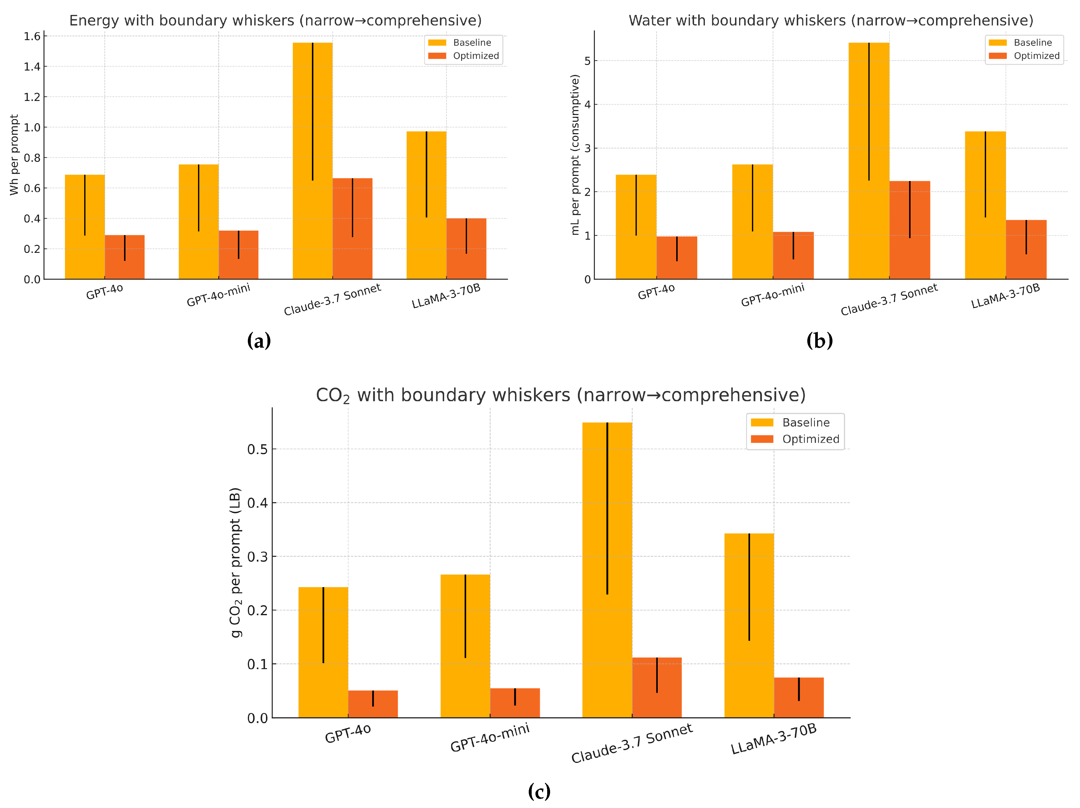
Figure 2.
Carbon–water movement at fixed QoS. For each model, the arrow connects the comprehensive-boundary medians from baseline to optimized. Lower whiskers mark accelerator-only values: energy and LB CO2 via the 0.417 energy ratio; water via source-only .
Figure 2.
Carbon–water movement at fixed QoS. For each model, the arrow connects the comprehensive-boundary medians from baseline to optimized. Lower whiskers mark accelerator-only values: energy and LB CO2 via the 0.417 energy ratio; water via source-only .
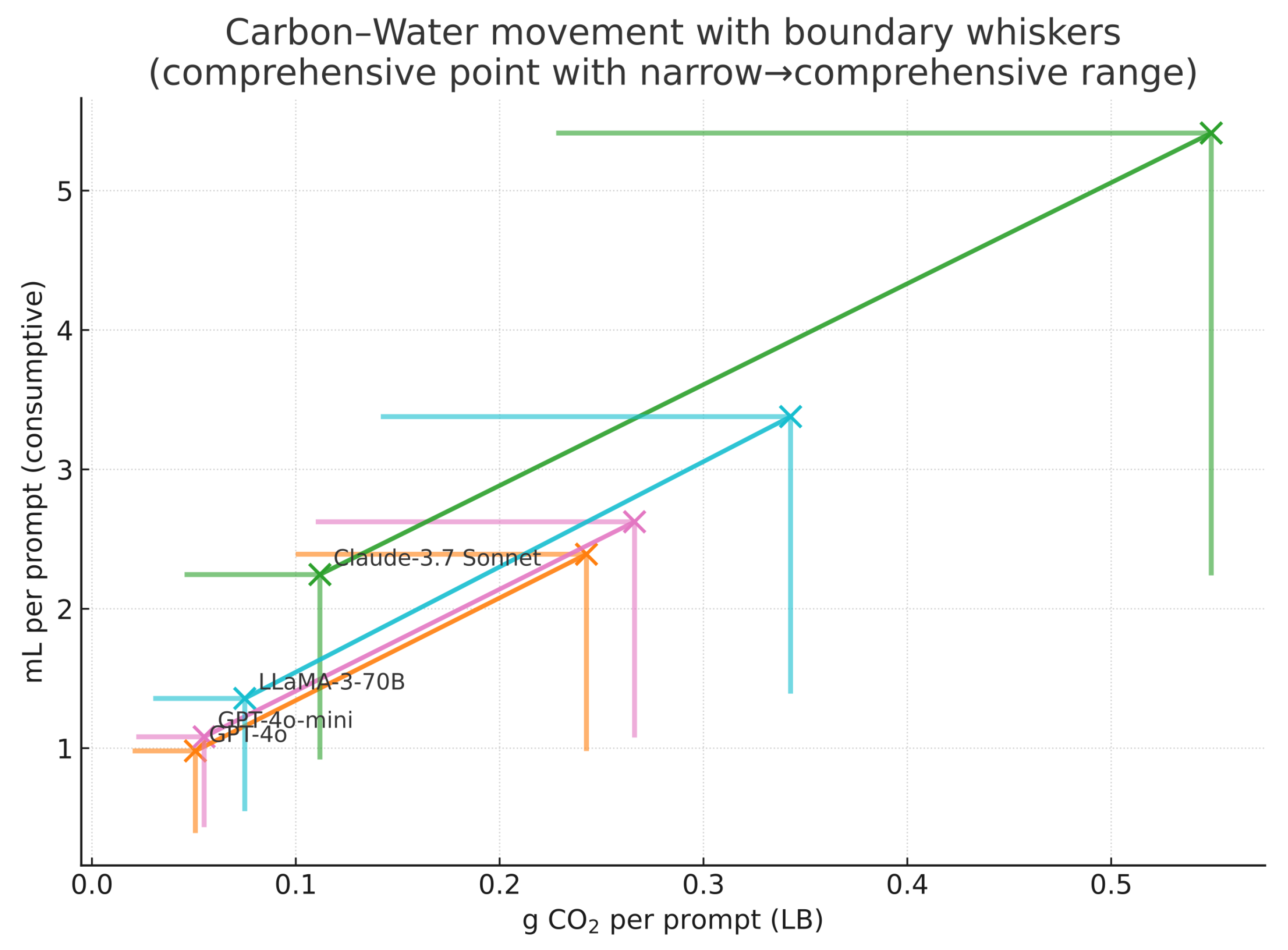
Figure 3.
Three-site routing Pareto with SLO (one panel per model). Each dot is a routing mix across a baseline U.S. thermal site, a hydro-dominated site, and a nuclear-like site, evaluated at the model’s optimized energy . Coordinates follow (17): and with. Gray points satisfy the p95 TTFT SLO (21); salmon points violate it. The red polyline is the lower-left Pareto frontier. Under hydro low but high , the efficient set is the hydro↔ nuclear edge; the baseline vertex is dominated (higher carbon and no water advantage).
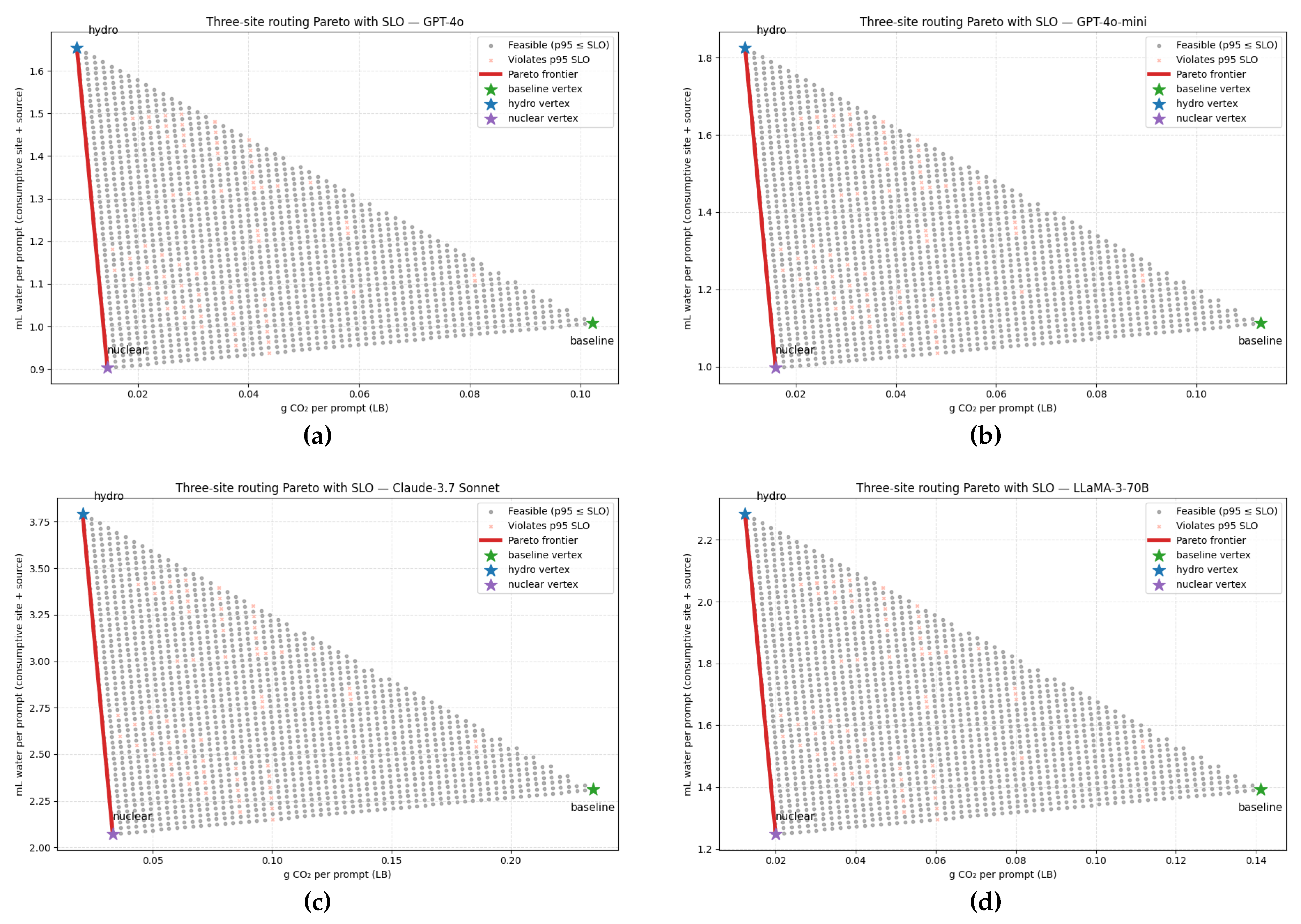
Figure 4.
Joint site + batch + token Pareto with SLO (one panel per model). Each dot corresponds to a triple of routing shares, batch multiplier, and token-length multiplier. Impacts follow (21): and , where and . Gray points satisfy the p95 TTFT SLO, salmon violate it. The red curve is the feasible lower-left Pareto frontier. Stars mark the single-site anchors at , which are dominated once batching and concise tokens are allowed. Relative to routing only, the feasible cloud becomes a wedge of scaled triangles and the frontier moves down and left, illustrating how operational levers compound with siting.
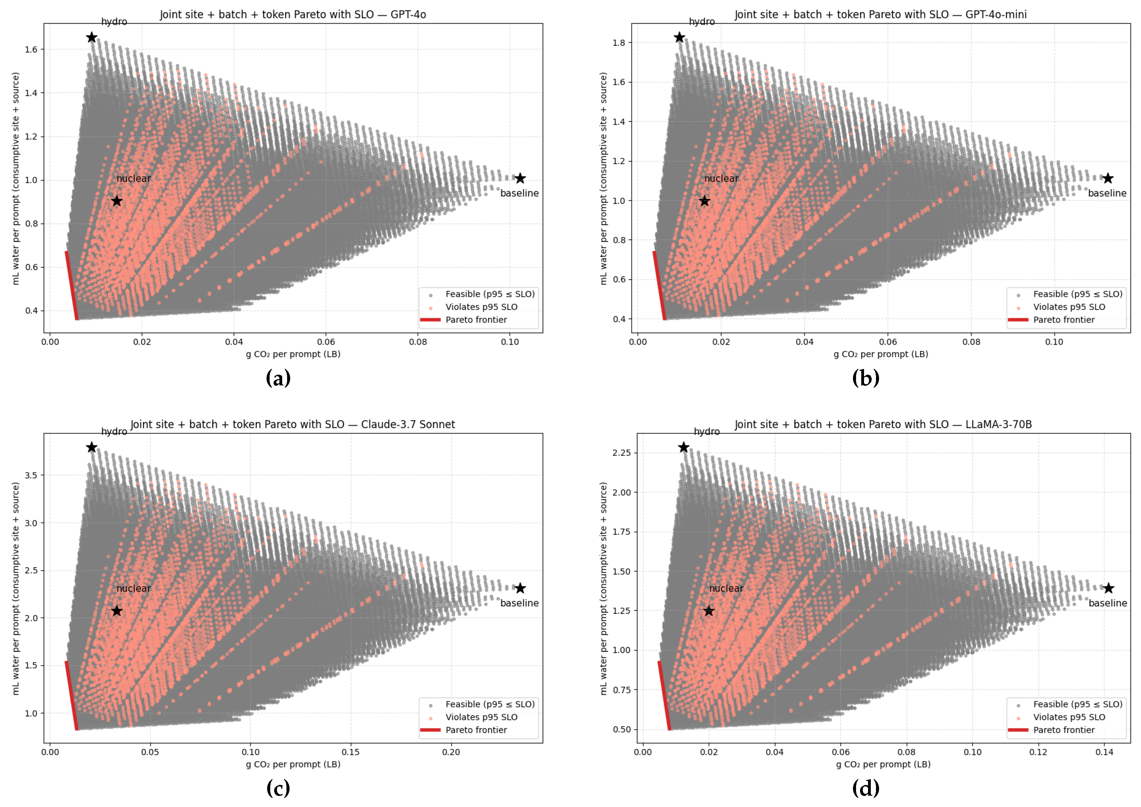
Figure 5.
Ablation A1—Routing-only, SLO overlay (GPT-4o). Feasible routing simplex in the plane at fixed optimized energy , with site factors (hydro: very low but higher ). Stars mark the three single-site vertices; ∘: p95-feasible; ×: p95-violating (mix proxy (21)). The red polyline is the lower-left Pareto frontier; it coincides with the hydro↔nuclear edge. Sensitivity whiskers at vertices: , (water), CIF (carbon) or LB↔MB when available.
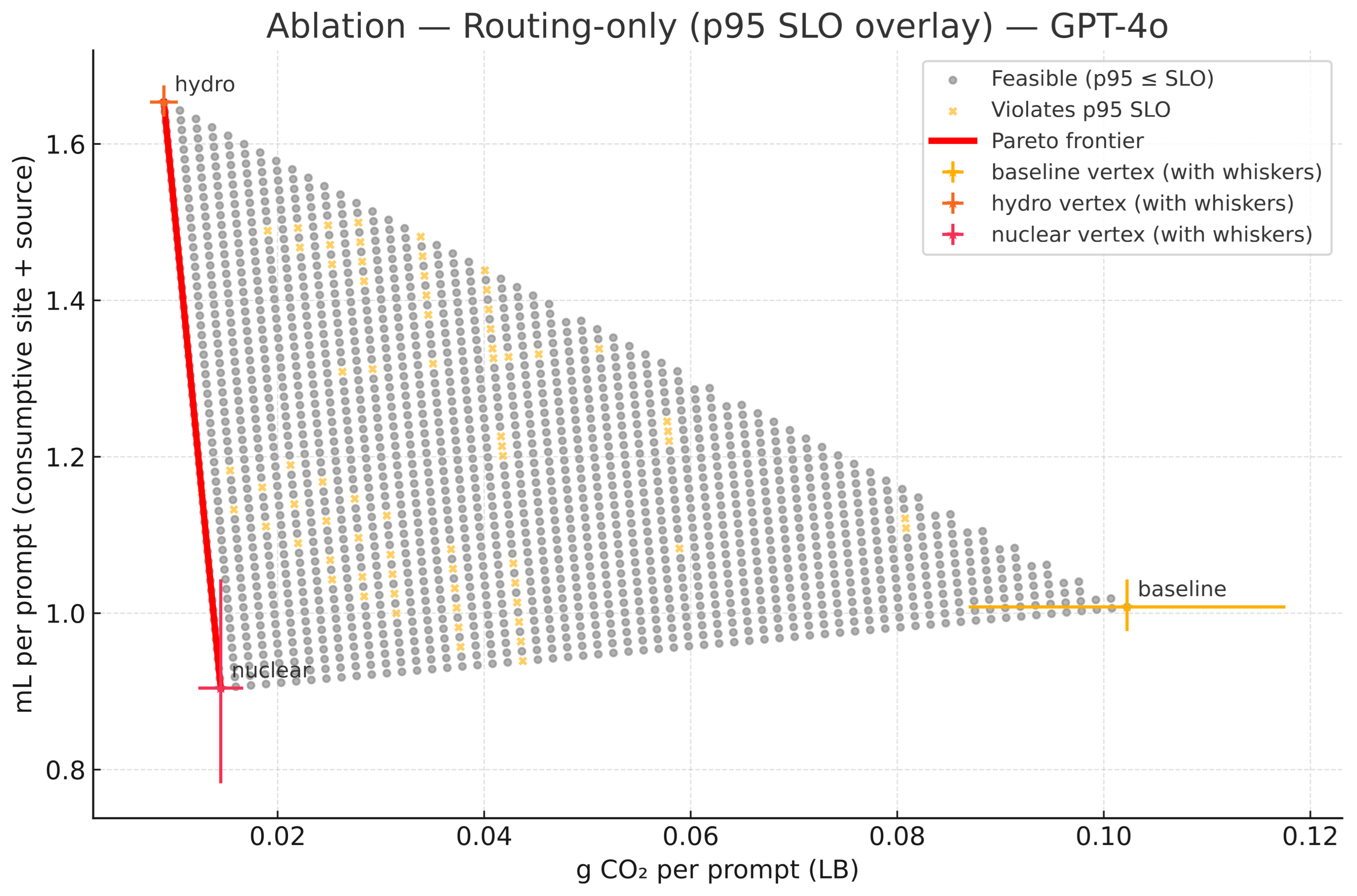
Figure 6.
Ablation A2—Routing + Batch, SLO overlay (GPT-4o). Adds a batch multiplier that scales energy and thus both axes by b while meeting p95 SLOs. The routing triangle thickens into a wedge of scaled triangles; the feasible red frontier shifts down-left relative to A1. Vertex whiskers as in Figure 5.
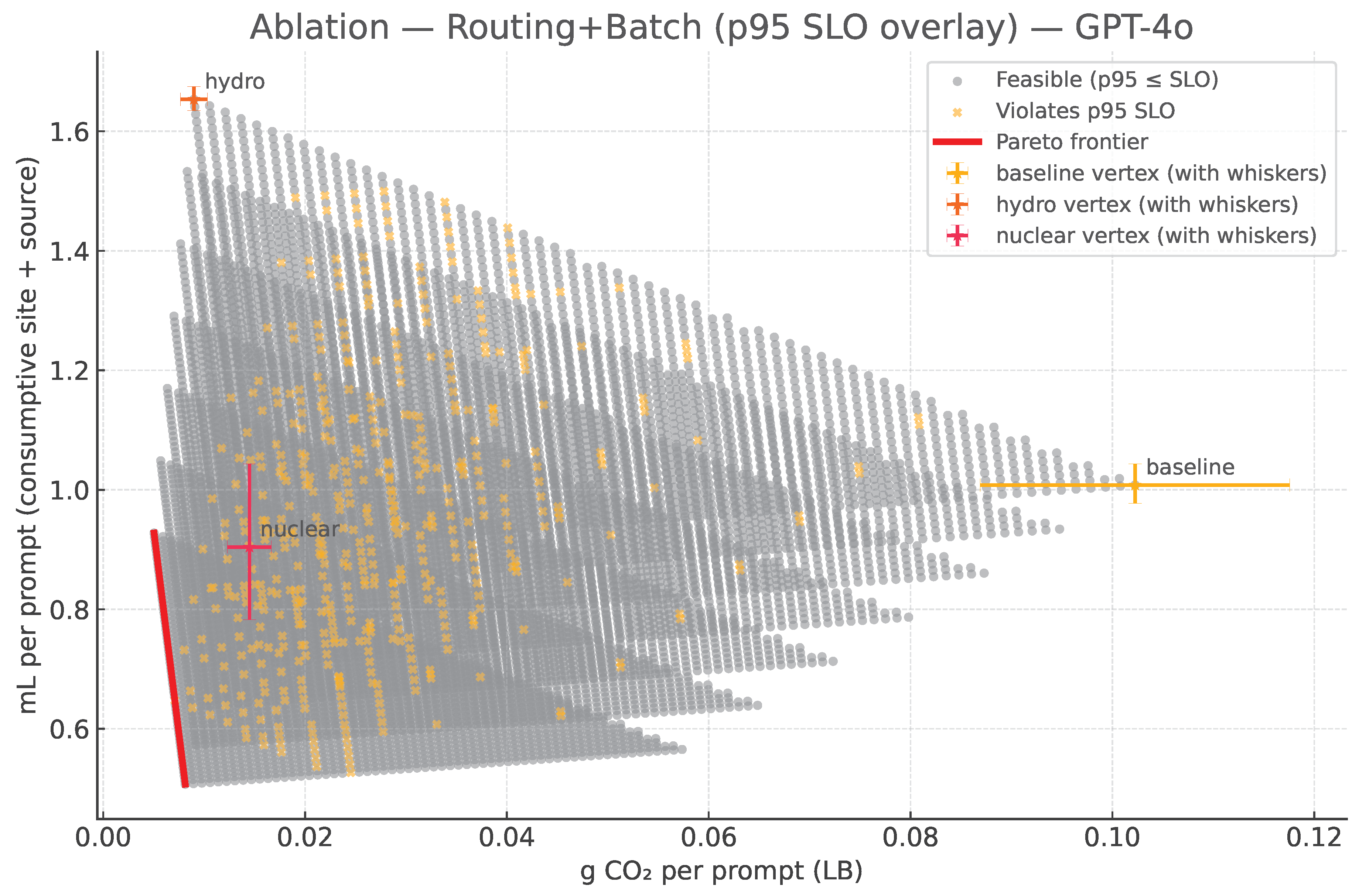
Figure 7.
Ablation A3—Routing + Batch + Token, SLO overlay (GPT-4o). Adds a token-length multiplier (default→brief), giving a uniform contraction on both axes (cf. ()). The feasible cloud expands and the lower-left frontier lengthens compared to A2; single-site stars at are dominated once batching and concise tokens are allowed. Vertex whiskers as in Figure 5.
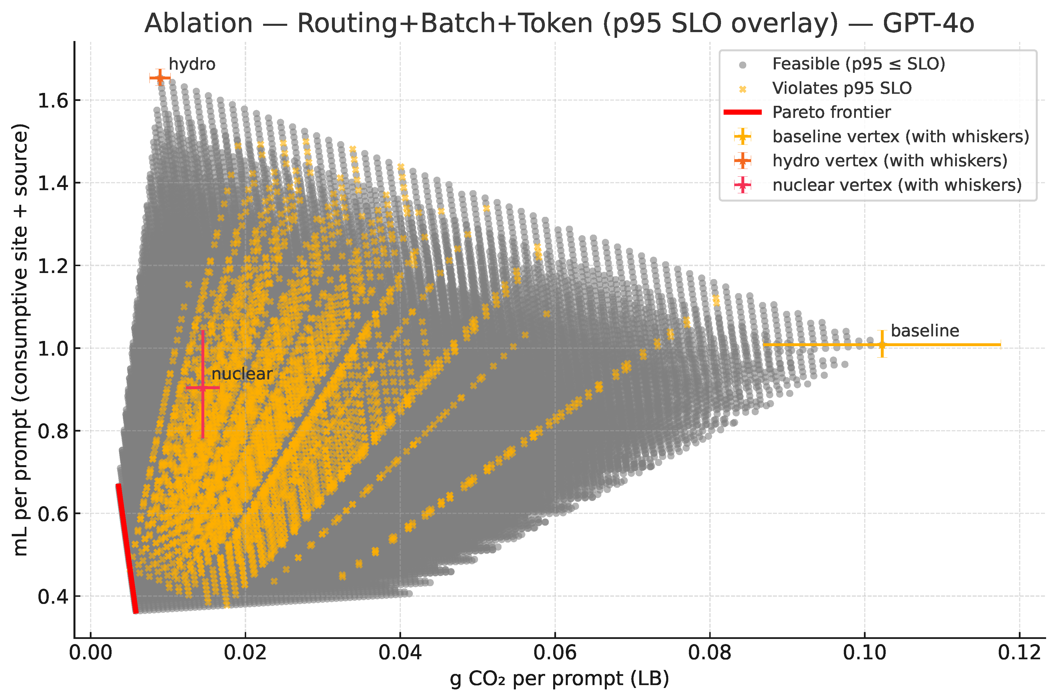
Figure 8.
Ablation A4—Routing + Phase split, SLO overlay (GPT-4o). Prefill (compute-bound) and decode (memory-bound) are allowed to run on different cohorts using phase-aware ; we sweep with default decode share . The feasible cloud nudges further down-left relative to A1; the hydro↔nuclear edge still sets the trade-off slope ((20)). Whiskers and SLO overlay as before.
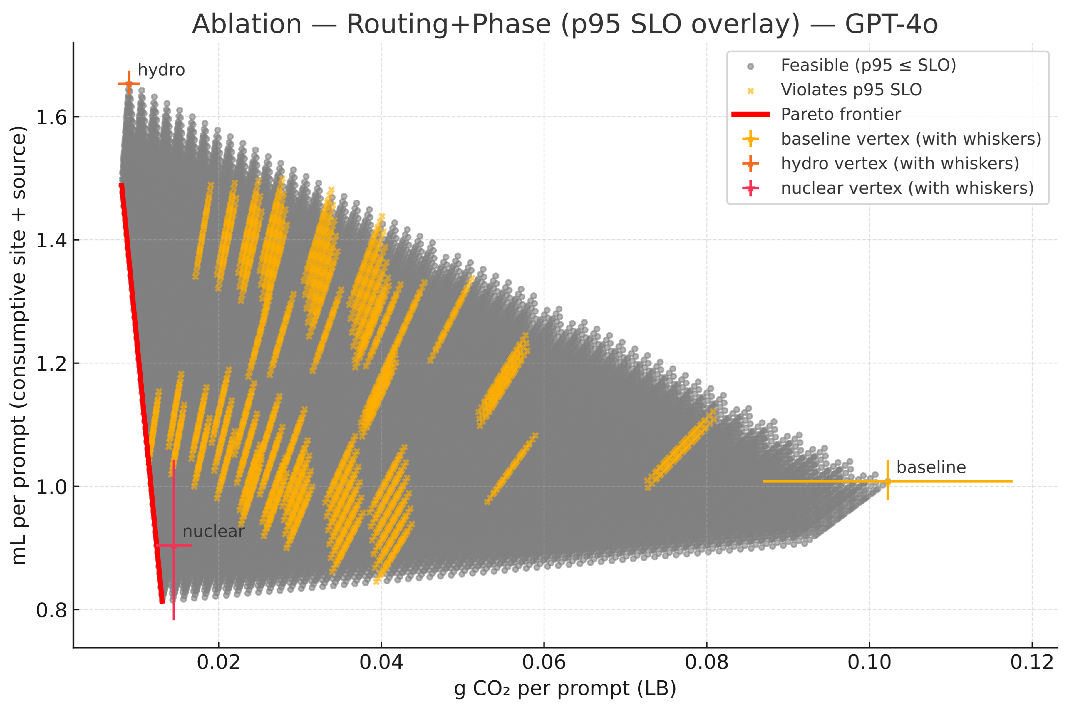

Table 1.
Comprehensive boundary medians (weighted by the mix).
| Metric | GPT 4o | GPT 4o mini | Claude 3.7 Sonnet | LLaMA 3 70B† |
|---|---|---|---|---|
| Baseline Wh/prompt | 0.6876 | 0.7545 | 1.55635 | 0.97145 |
| Optimized Wh/prompt | 0.289824 | 0.319896 | 0.664582 | 0.400321 |
| Energy % | ||||
| Baseline mL/prompt | 2.391473 | 2.624151 | 5.412985 | 3.378703 |
| Optimized mL/prompt | 0.980349 | 1.081547 | 2.245570 | 1.356734 |
| Water % | ||||
| Baseline g CO2/prompt (LB) | 0.242585 | 0.266188 | 0.549080 | 0.342728 |
| Optimized g CO2/prompt (LB) | 0.050739 | 0.055035 | 0.111840 | 0.074971 |
| CO2 % | ||||
| Baseline Energy (GWh/d) | 0.3438 | 0.37725 | 0.778175 | 0.485725 |
| Optimized Energy (GWh/d) | 0.144912 | 0.159948 | 0.332291 | 0.200160 |
| Baseline Water (ML/d) | 1.196 | 1.312 | 2.706 | 1.689 |
| Optimized Water (ML/d) | 0.490 | 0.541 | 1.123 | 0.678 |
| Baseline CO2 (t/d, LB) | 121.293 | 133.094 | 274.540 | 171.364 |
| Optimized CO2 (t/d, LB) | 25.370 | 27.517 | 55.920 | 37.485 |
† Long-prompt Wh for LLaMA 3 70B is not reported in the public table; the line aggregates short+medium medians and is flagged accordingly. Units: 1 ML L mL. At 500 M prompts/day, ML/d mL/prompt; GWh/d Wh/prompt; t/d g/prompt.
Table 2.
Accelerator-only vs. comprehensive (medians, mix).
| Metric | GPT 4o | GPT 4o mini | Claude 3.7 Sonnet | LLaMA 3 70B |
|---|---|---|---|---|
| Narrow Wh/prompt | 0.2865 | 0.314375 | 0.648479 | 0.404771 |
| Comprehensive Wh/prompt | 0.6876 | 0.7545 | 1.55635 | 0.97145 |
| Narrow/Comprehensive | 0.417 | 0.417 | 0.417 | 0.417 |
| Narrow mL/prompt | 0.996447 | 1.093396 | 2.255411 | 1.407793 |
| Comprehensive mL/prompt | 2.391473 | 2.624151 | 5.412985 | 3.378703 |
| Narrow g CO2/prompt (LB) | 0.101077 | 0.110911 | 0.228783 | 0.142803 |
| Comprehensive g CO2/prompt (LB) | 0.242585 | 0.266188 | 0.549080 | 0.342728 |
Disclaimer/Publisher’s Note: The statements, opinions and data contained in all publications are solely those of the individual author(s) and contributor(s) and not of MDPI and/or the editor(s). MDPI and/or the editor(s) disclaim responsibility for any injury to people or property resulting from any ideas, methods, instructions or products referred to in the content. |
© 2025 by the authors. Licensee MDPI, Basel, Switzerland. This article is an open access article distributed under the terms and conditions of the Creative Commons Attribution (CC BY) license (http://creativecommons.org/licenses/by/4.0/).
Copyright: This open access article is published under a Creative Commons CC BY 4.0 license, which permit the free download, distribution, and reuse, provided that the author and preprint are cited in any reuse.


