
Submitted:
09 October 2025
Posted:
10 October 2025
You are already at the latest version
Abstract
The Nyquist Folding Receiver is an architecture that uses Compressed Sensing to convert analog Radio Frequency signals into digital signals. Analog-to-Digital Converter architectures that implement Compressed Sensing are collectively known as Analog-to-Information. Sparse bandlimited analog signals with frequency bands above the Nyquist frequency of a traditional Analog-to-Digital Converter can be recovered by Analog-to-Information receivers. Recovery of these signals is affected by the selection of a Compressed Sensing recovery algorthim. Typical recovery algorithms selected for recovery of Nyquist Folding Receiver compressed outputs use iterative methods to find the solution. This work presents a machine learning approach to signal reconstruction. The proposed method uses a neural network to learn the mapping from compressed samples to the original signal. The neural network is trained on a set of synthetic signals generated by a new open-source Analog-to-Information simulator called SpectraMelt. The results show that the neural network can effectively reconstruct the original signal from the compressed samples, achieving better performance than traditional iterative methods.
Keywords:
analog-to-digital
; analog-to-information
; cognitive radio
; compressed sensing
; Nyquist Folding Receiver
; radio frequency
1. Introduction
Modern information systems (IS) increasingly demand acquisition rates that strain existing hardware, as Nyquist-rate sampling of high-bandwidth signals produces excessive data or imposes impractical capture requirements. The Analog-to-Digital Converter (ADC) is a central bottleneck in this process. A major shift came with Donoho’s 2006 introduction of Compressed Sensing (CS) [1], which offered a framework to bypass Nyquist constraints. CS exploits the structure of finite-dimensional inner product spaces by employing the norm to promote sparsity, enabling accurate reconstruction of certain signals from sub-Nyquist samples.
This breakthrough inspired extensive research into Analog-to-Information (A2I) converters (Figure 1) [7], architectures that embed CS principles directly into data acquisition. Notable A2I designs include the Random Demodulator (RD) [2], the Modulated Wideband Converter (MWC) [3], and the Nyquist Folding Receiver (NYFR) [4]. While none yet rival traditional ADCs due to performance trade-offs [5], the NYFR remains a leading candidate for sub-Nyquist sampling.
Early modeling work [14] is extended here with a neural network-based reconstruction framework that improves both theoretical accuracy and empirical performance, significantly narrowing the gap between experimental feasibility and practical deployment by surpassing traditional iterative methods on real-world signals. The neural network is enabled by an open-source A2I simulator called SpectraMelt. This new simulator allows for the creation of A2I digital twins that can generate synthetic data needed for the training of the network without the need for hardware implementation while promoting the development of new A2I architectures.
Figure 1.
General A2I Sampling Architecture
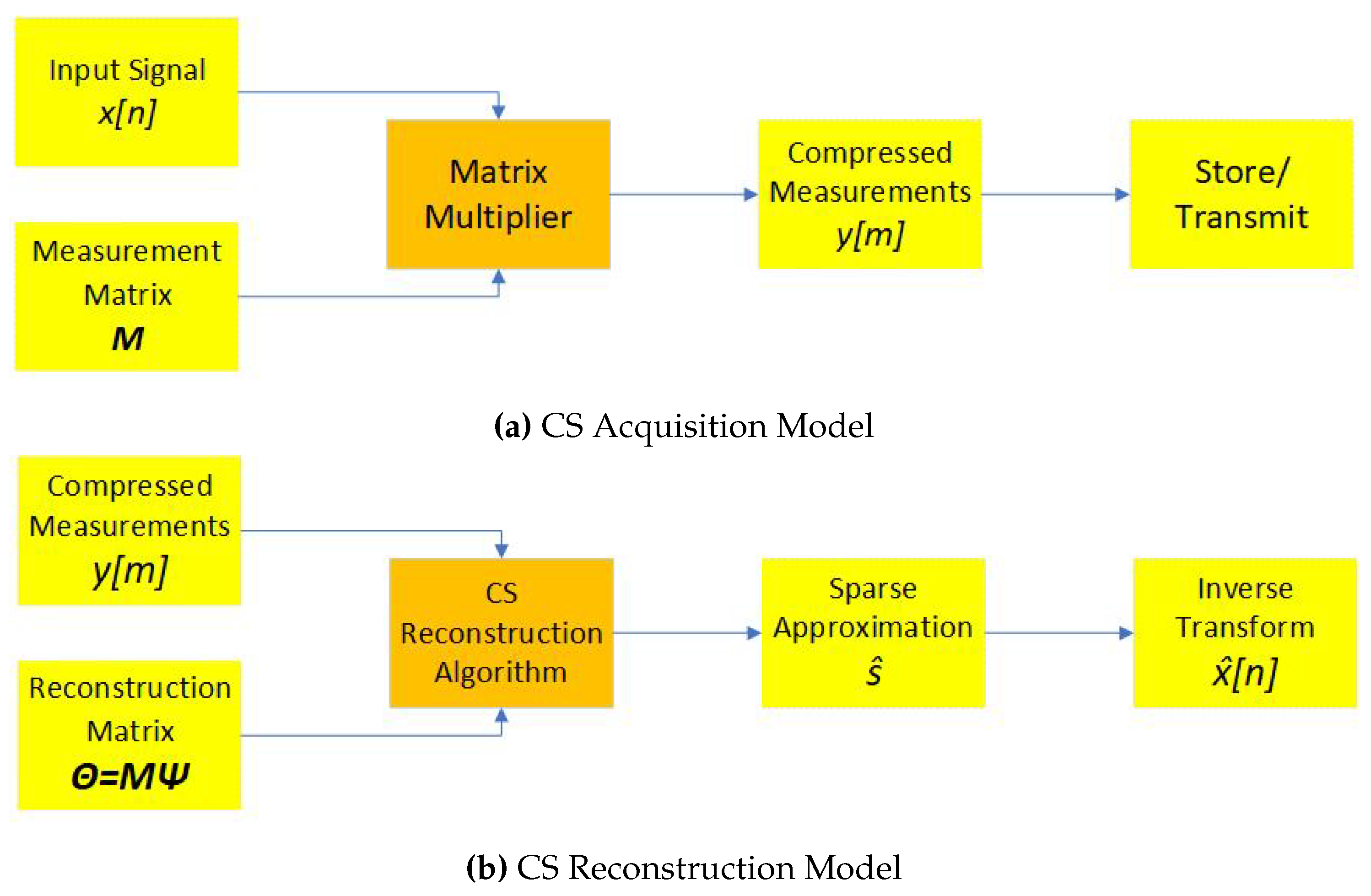
1.1. Compressed Sensing Background
While a full treatment of CS theory is beyond the scope of this work, a brief overview is provided to establish the mathematical foundations, recovery conditions, and assumptions that justify the signal model. In CS, a vector of length N belongs to , typically with . An inner product space defines the norm as , with the general norm given by:
For these are quasi-norms. At , , where denotes the indices of nonzero elements. norms measure approximation error between and its estimate as . CS exploits sparsity, especially with the norm, since errors concentrate in fewer coefficients. A signal of length N with at most K nonzeros () is K-sparse where . Many signals become sparse in Fourier or Wavelet bases. If is sparse when transformed by a universal basis where satisfies , it is called compressible.
For a compressible , CS allows reconstruction from measurements :
where P is the number of measurements, is the measurement matrix, , and . This holds when contains Gaussian or Bernoulli random variables.
Since (1) is underdetermined, recovery seeks the sparsest by solving:
where argmin finds minimizing . This NP-hard problem can be relaxed to a convex -minimization if satisfies the Restricted Isometry Property (RIP), again true for Gaussian or Bernoulli cases.
1.2. The Nyquist Folding Receiver
The NYFR folds RF subspaces using a modulated local oscillator (LO)
with angular frequency . The narrowband modulation satisfies and is defined as
This sweeps the LO frequency across , requiring where Q is a positive integer to maintain RIP [9]. A pulse train from LO zero crossings can be expressed as
where modulation disrupts uniform spacing. Multiplying by the wideband input applies the Nyquist-Shannon theorem, folding components into the LO-defined baseband consistent with the Union of Subspaces (UoS) model [13].
Figure 2.
Nyquist Folding Receiver Block Diagram
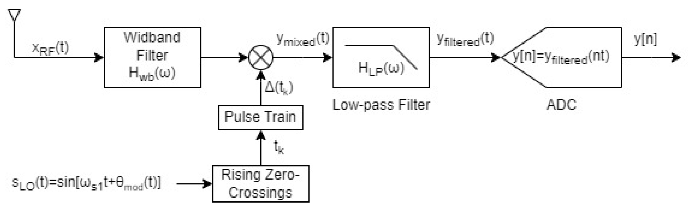
Mixing produces with baseband frequencies
A low-pass filter with cutoff
suppresses aliases, yielding with induced modulation , where M is an integer scale factor. Finally, a conventional ADC samples at , near but not equal to the average rate of , producing where . This last stage acts like time-domain decimation, multiplying by the ADC’s sampling train without introducing new modulation.
Figure 3.
Real Valued Sampling Model for the NYFR.
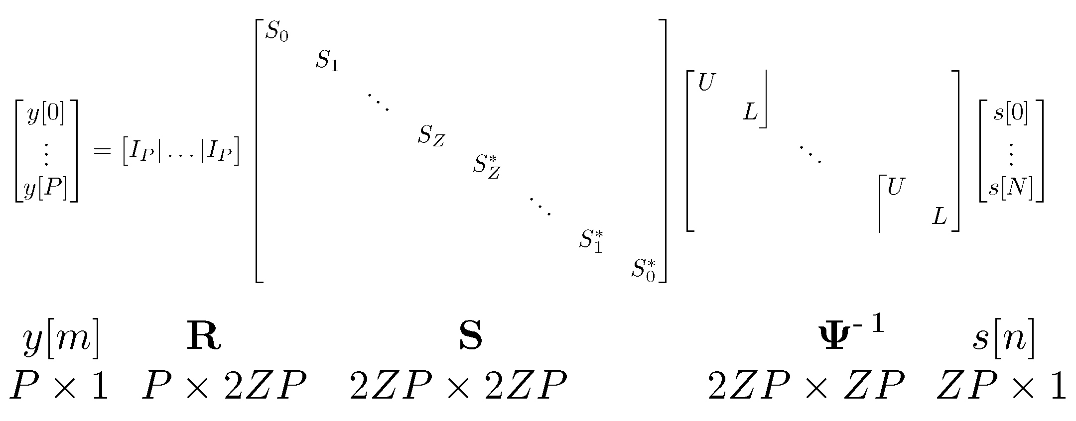
Once the compressed input signal is collected, a CS algorithm reconstructs the original signal from measurements, as shown in Figure 1. Reconstruction accuracy depends on the reconstruction matrix , which serves as input to the CS recovery for the NYFR as shown in Fig. [10]. The NYFR Sampling Model specifies vector and matrix dimensions: P measurements by the ADC, and the measurement vector. The number of positive folds relates Nyquist frequency and LO frequency by , set by the Wideband Filter cutoff . For example, if and , then . The universal basis is Fourier , so . The inverse transform is a block diagonal matrix with blocks D formed from sub-blocks U and L:
where .
The measurement matrix , where projects Z NYFR zones onto baseband of P samples, and is a conjugate symmetric diagonal matrix modulating each zone over time. Each sub-block , where contains sampled LO elements at ADC sample times . The modulation index defines the original signal frequency and peak deviation , with sign indicating sideband and a 90° shift for negative modulation. Thus, comprises two conjugate symmetric blocks with the common time modulation pattern scaled by each zone’s M value.
2. SpectraMelt
The promise of CS to recover sampled signals having bandwidths beyond the Nyquist frequency has led to extensive research on A2I architectures, with numerous designs proposed to reduce power consumption compared to traditional ADCs [15]. While current A2I implementations do offer measurable power savings, conventional ADC architectures still surpass them in terms of achievable sampling rates [5]. For A2I technology to move beyond experimental use and achieve mainstream adoption, it will be essential to identify and refine the most capable designs. Modeling and simulation play a critical role in this process, enabling not only rigorous comparison of candidate architectures but also the exploration of hybrid approaches that combine the strengths of multiple methods. Furthermore, simulation provides a foundation for developing innovative signal recovery algorithms, ultimately helping to close the performance gap between A2I converters and traditional ADCs. The NYFR was selected for simulation because of compelling qualitative analysis done here [6].
Simulation requires the application of models within a virtual RF signal environment. There are multiple platforms available for generating these virtual environments, with Matlab being a popular choice due to its flexibility and speed through the use of specialized toolboxes. Its widespread adoption is exemplified by its use in the analysis done here [10]. However, Matlab’s reliance on costly licensing restricts code sharing between large companies and academic institutions. In contrast, open source software and open architectures promote free sharing and collaborative development, which accelerates progress and enhances security by exposing the software to a broad community. The downside is that open source projects may lack formal support unless actively maintained, unlike Matlab’s paid support model.
Because of these considerations, an open source model was selected for this work. Among existing options, GNURadio stands out as a mature framework widely used across research, industry, and academia for software-defined radio (SDR) applications and simulations. Built on Python, GNURadio offers a rich library of signal processing blocks enabling complex transmit and receive architectures. Yet, its simulated environment has limitations, such as timing mismatches causing spurious frequency signals and limited environmental control, which constrain detailed testing of A2I architectures. To overcome these issues while leveraging Python’s flexibility and compatibility with GNURadio, a custom RF simulator directly implemented in Python is proposed for greater environmental control and integration with neural network tools.
This simulator began development here [14] with the creation of a NYFR digital twin to establish functionality. However, attempted reconstruction using several different CS recovery algorithms yielded inaccurate results. A refactoring of the code into more traditional object oriented methods was needed before a root-cause analysis could be conducted. By refactoring the code, a more mature simulator was now available for testing, dubbed SpectraMelt v1. A class diagram of the NYFR implementation is shown in Figure 4.
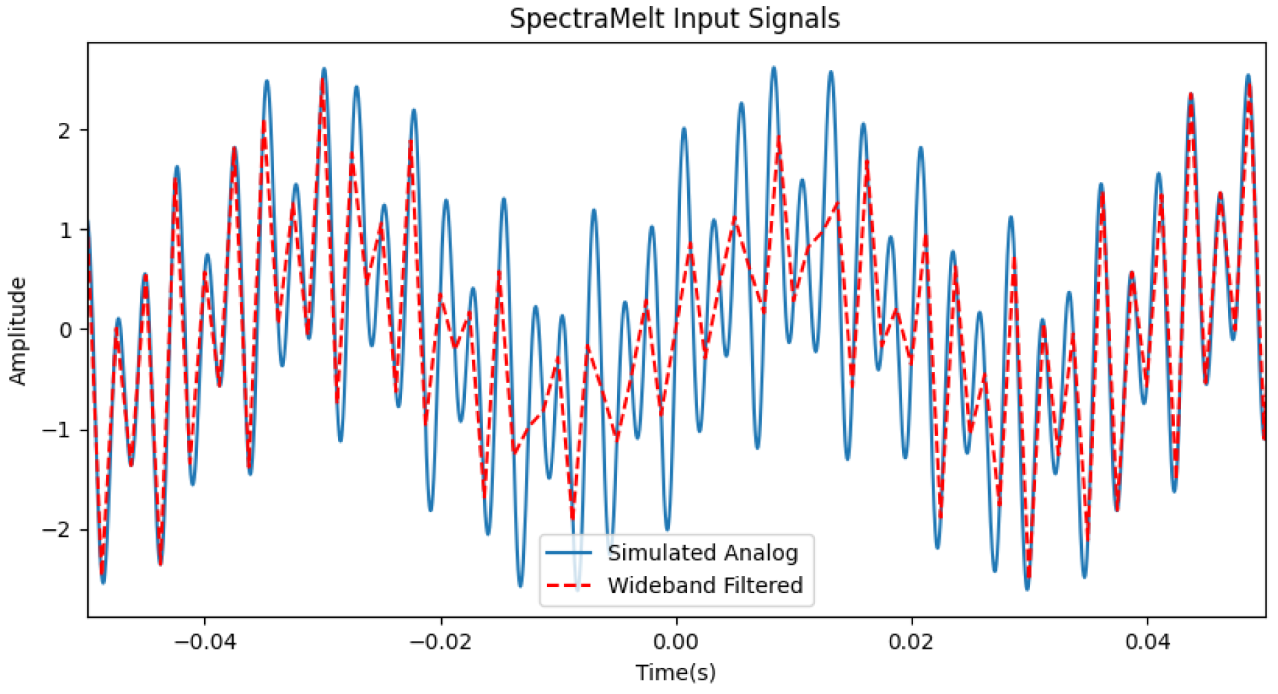
Unit testing against SpectraMelt followed the sequence diagram shown in Figure 6. This testing, along with expert advice, led to the discovery that the frequency of the underlying simulator time was not sufficient to represent analog signals. Originally, input signals leaving the wide-band filter were used as the simulator time base. By creating an `analog’ input signal using a vector with time steps much smaller than the one originally used for the output from the wide-band filter, overall fidelity of SpectraMelt was improved. Figure 5 gives an example of how the input signal shape in the time domain more accurately represents an analog signal at this time scale verses the original version, highlighting the importance of selecting an appropriate simulator frequency.
Figure 5.
Simulated Analog vs. Wideband Filtered 1MHz vs. 400Hz Input Tones at 25Hz, 255Hz, and 395Hz
Figure 5.
Simulated Analog vs. Wideband Filtered 1MHz vs. 400Hz Input Tones at 25Hz, 255Hz, and 395Hz
3. Improved A2I Recovery
Now that SpectraMelt is producing accurate compressed samples, the next step is to show how it can be leveraged to improve A2I designs. One way to do this is to produce a new CS recovery method within the simulator that exceeds current, state-of-the practice, traditional iterative CS recovery methods in terms of speed and recovery accuracy. Machine Learning (ML) is a signal processing technique that has exploded in popularity in recent years. The most successful ML technique has been the Artificial Neural Network (ANN) originally developed by psychologist Frank Rosenblatt in 1958 [16]. While ANNs have been applied to virtually every problem space thanks to the rise of Large Language Models (LLMs), only recently have they been applied to A2I. In 2023, a team from the University of Electronic Science and Technology of China used LLMs to try and classify the compressed output of the NYFR against a group of Radar signal types [17].
The ANN chosen for implementation within SpectraMelt to decompress NYFR outputs is called the Multilayer Perceptron (MLP). A MLP is a simple feedforward network that maps fixed-size inputs to outputs, while a LLM is built on the transformer architecture with self-attention, enabling it to capture long-range dependencies and contextual relationships in variable-length sequences. The architecture of the MLP implemented here is modeled after a more advanced architecture inspired by sparse Bayesian learning (SBL) called Learned-SBL [18]. This new network contains an input layer, one hidden layers, and one output layer. Each layer is fully connected with the previous layer. The input layer contains the same number of inputs as the number of samples captured at the simulated output of the NYFR. The hidden and output layer perceptrons all contain the same number outputs as the uncompressed input signal. A toy example with four nodes per layer is shown in Figure 7
Typical activation functions such as the Rectified Linear Unit (ReLU) are applied to perceptron outputs when the network is performing classification tasks, constraining the value between zero and one. Because the network uses unsupervised training, the output from an MLP layer cannot be constrained this way, leading to the activation function given by
This means that the output from each layer is just a linear combination of the inputs from the previous layer.
Another consideration is the type of Loss Function used to train the network during back-propagation. Initially, a mean absolute error (MAE) loss function was selected as it calculates the average of the absolute differences between predictions and true values. This seemed in line with the traditional CS principle from eq. 2 where the recovery problem is relaxed to a convex -minimization problem by setting . In reality, this spred the error for the training over every output node, resulting in no signal recovery, only output noise. A custom root mean squared error (RMSE) function given by:
was created for the network to get the desired results.
3.1. Dataset Creation
With a working MLP implementation in place, it was time to create datasets from the NYFR digital twin. These datasets would serve three purposes:
- Training data for the new MLP
- Signals used for recovery to assess MLP performance verse other CS recovery algorithms
- Assess the impact of varying NYFR LO parameters on data recovery
The datasets were created as an extension of the simulator settings found here [14], with 1MHz, 400Hz, 100Hz, 100Hz, 50Hz, -2s, and 2s. This sets the number of positive Nyquist Zones .
Each input dataset was generated from a list of all the possible integer input frequencies that can exsist within the wide-band filter range. In this case, the possible frequencies where , , …, , giving the total number of possible frequencies . Every is comprised of input signals with tones drawn from and taken n at a time with resulting in a total of four sets containing 79800 signals per set. The individual tones within each input signal had random amplitudes between 0.5 and 1 taken from a uniform random variable. The input signals created in these initial datasets are idealized to show functionality of SpectraMelt and quickly compare implemented recovery algorithms. This means that no noise is added to them and signal tones are expressed as linear measures of magnitudes instead of the typical dB.
Recovery algorithms for the NYFR are directly influenced by how the LO parameters are tuned, since these parameters govern the modulation index and resulting frequency zone definitions. Specifically, the modulation index M uniquely determines the mapping of signals into frequency zones, but it is only valid under the condition that the clock modulation remains narrowband. This requires the maximum rate of change of , given by
to be much smaller than . In practice, this translates to at least two orders of magnitude separation between the modulation deviation and the local oscillator frequency . Furthermore, the system is typically constrained such that , tightly linking the oscillator design to the sampling process and imposing additional structure on the recovery algorithms.
Selection of specific LO parameters within the current literature relies on Monte Carlo simulations to select appropriate values within the constraints given above [10]. This search was done by first developing some qualitative analysis about LO parameter selection and then using recovery results from a single CS recovery algorithm. Understanding how to select appropriate LO parameters also requires understanding how the LO signal modulation affects the shape of the modulated pulse train in both time and frequency domains using the analysis performed here [14]. The modulation frequency must be tuned to match the size of the zones created by the NYFR with some integer multiple of the width of the LO frequency domain lobes. The matching of lobe widths will reduce mutual coherence between zones, increasing recovery accuracy.
Beyond the analysis and constraints to the LO parameters just described, there is currently no prescription on which specific values to select for and given and , meaning that some Monte Carlo simulations are still required. On top of that, there has been little analysis to determine if these values are specific only to one selected CS recovery algorithm. SpectraMelt help address these issues by generating datasets for the NYFR with varying LO parameters of the digital twin. For the system parameters used to create each , the following list of LO parameters was used to create 16 unique datasets: , , , , . These LO parameters were also used to create CS recovery dictionaries needed for reconstruction based on Figure 3.
3.2. Compressed Data Recovery
Improvements to based on comparisons between the actual output of the NYFR Digital Twin and the approximation given by was discussed here [14]. However, this approach is flawed. What is really needed is adjustments based on the initial guess where is the pseudoinverse of the NYFR recovery dictionary. Graphical examination of applied to Digital Twin outputs shows that orientation mismatches are corrected using the pseudoinverse. The magnitude discrepancies are also corrected within iterative CS algorithms by normalizing the ouput . To correct for magnitude mismatches within the MLP training data and improve reconstruction speed, is created by pre-multiplying the measurement matrix with a magnitude correction factor to give . This correction factor was determined by trial and error. An example signal is shown in Figure 8.
There is a need to systematically compare the performance of this new MLP network against the previous state-of-the-art iterative CS recovery methods. Orthogonal Matching Pursuit (OMP), Spectral Projected Gradient for L1 minimization (SPGL-1), and Iterative Hard Thresholding (IHT) were added to SpectraMelt as the state-of-the-practice methods because of their relative successes in CS recovery. The OMP algorithm used for reconstruction was modified from the original algorithm within the Scikit-Learn Python library to allow for complex valued dictionaries. A custom complex version of IHT was also created based on [19]. SPGL-1 reconstruction was implemented using the SPGL1 Python library found in the PyPi repository.
The input and output datasets from the previous section have been recovered using four separate CS recovery algorithms incorporated into SpectraMelt: IHT, OMP, SPGL1, and the newly trained MLP network. Several assumptions about the recovery results should be mentioned before discussing the recovery results. One is that the IHT algorithm was given the correct number of unknown tones a priori. This was done for baseline results, as IHT is the oldest of the four algorithms. No other algorithm had this knowledge. Secondly, an individual MLP network was trained per signal set, for a total of four networks. These networks only recovered signals with the corresponding number of tones per signal. This was done because the training of the same MLP on different datasets caused catastrophic forgetting, a well-known limitation of MLPs when trained on tasks sequentially.
For each recovery set, several metrics were used to assess the quality of the recovered signals. In order for a signal tone to be considered recovered, it must first exactly match one of the input tone frequencies. If the magnitude exceeds half of the original tone’s magnitude, then the signal tone is marked as recovered. If any recovered signal also exceeds this threshold but does not match an input tone frequency, it is considered a spur. The average magnitude error of the recovered signals is considered along with the average magnitude of the spurs. The recovery accuracy is found by dividing the number of recovered signals by the total number of input signals. The spur rate divides the total number of spurs by the total number of input signals. An example of signal recovery from each recovery method in SpectraMelt is shown in Figure 9
One of the broad questions that this work is trying to answer is “What are the specific NYFR LO settings that maximize reconstruction?” From the results obtained by the three iterative algorithms, no effect on signal recovery was seen by varying LO parameters. However, there were variations seen from the MLP recovery results which seemed to favor . No accompanying variations were seen by different values with the previous frequency across all datasets. It should be noted that the standard deviation in recovery accuracy between different datasets and LO parameters never exceeded 0.009 from the MLP recovery results. These results together seem to suggest that there is no preferable LO parameter setting as long as the previously stated constraints are held. This matches the previous analysis done showing that and jointly constrain the system’s dynamic reconstruction range, balancing signal recovery, zone identification, pulse resolution, and phase-noise limitations [10].
Table 1 shows the compiled results from the NYFR digital twin simulations using the datasets described in the previous two sections. All reported values are averages over 100 recovered signals. This table shows a clear distinction between the IHT and OMP algorithms. The a priori knowledge given to the IHT improved the average spur rate produce by the algorithm. It did not, however, improve the reconstruction accuracy, as this is the main measure of a selected CS algorithms performance. This shows that the OMP is a better CS algorithm for the NYFR than the IHT. There is also a clear distinction between the two older algorithms, IHT and OMP, versus the newer two, SPGL1 and MLP, in terms of recovery accuracy. Of final note, the MLP networks recovery accuracy is on average about double that from SPGL1, 63.8% vs 38.3%, while almost completely eliminating spurs.
4. Conclusion and Future Work
The previous analysis demonstrates the superiority of the new MLP-based recovery method over state-of-the-practice CS recovery techniques, while underscoring the importance of modeling and simulation in advancing A2I architectures. Digital twins enable the design of novel recovery algorithms and exploration of alternative A2I architectures. The open-source nature of SpectraMelt will allow researchers to rapidly prototype and evaluate new designs, accelerating adoption of A2I as NYFR recovery accuracy improves. The GitHub repository https://github.com/pandas0517/A2I will be made public once SpectraMelt is finalized, inviting further contributions from motivated collaborators.
A limitation of the MLP approach is the potentially long training time, though most of this cost is concentrated in generating the pre-multiplication initial guess. Loading new dictionaries into a signal processing chain should be manageable, except when hardware implementation is required. In practice, alternative LO settings may not even be necessary. Techniques such as Learned-SBL could enable adaptive behavior, while dataset mixing strategies can mitigate catastrophic forgetting, enabling a single MLP model to recover multiple signal tones.
More representative NYFR datasets can be generated by incorporating environmental effects such as additive white Gaussian noise (AWGN), phase noise, and signal tones in realistic ranges (e.g., 2–3 GHz). Non-integer input frequencies should also be included, with input magnitudes and recovered outputs expressed in dB to better capture signal-to-noise relationships. An enhanced NYFR digital twin can further model quantization effects in the ADC, allowing metrics such as SINAD and ENOB to be computed. Testing the MLP on signals beyond five tones will demonstrate its generalization capability. The flexibility of SpectraMelt also supports compound A2I architectures, such as the Nyquist Folding Wavelet Bandpass Sampler (NFWBS), which combines the NYFR with the Non-Uniform Wavelet Bandpass Sampler (NUWBS) [20]. This architecture can be validated within SpectraMelt by implementing its CS measurement model and verifying signal reconstruction.
References
- D. L. Donoho, "Compressed Sensing," IEEE Transactions on Information Theory, pp. 1289-1306, 2006.
- S. Kirolos, J. Laska, M. Wakin, M. Duarte, D. Baron, T. Ragheb, Y. Massoud and R. Baraniuk, "Analog-to-Information Conversion via Random Demodulation," in IEEE Dallas Circuits and Systems Workshop on Design, Applications, Integration and Software, Richardson, TX, 2006.
- M. Mishali and Y. Eldar, "From Theory to Practice: Sub-Nyquist Sampling of Sparse Wideband Analog Signals," IEEE Journal of Select Topics in Signal Processing, vol. 4, no. 2, pp. 375-391, 2010. [CrossRef]
- G. L. Fudge, R. Bland, M. Chivers, S. Ravindran, J. Haupt and P. E. Pace, "A Nyquist Folding Analog-to-Information Receiver," in Asilomar Conference on Signals, Computing, and Systems, Pacific Grove, California, 2008.
- M. Torlak and W. Namgoong, "Spectral Detection of Frequency-Sparse Signals: Compressed Sensing vs. Sweeping Spectrum," IEEE Access, pp. 30060-30070, 2021.
- R. Maleh, G. Fudge, F. Boyle and P. Pace, "Analog-to-Information and the Nyquist Folding Receiver," IEEE Jounal on Emerging and Selected Topics in Circuits and Systems, vol. 2, no. 3, pp. 564-578, 2012. [CrossRef]
- M. Rani, S. B. Dhok and R. B. Deshmukh, "A Systematic Review of Compressive Sensing: Concepts, Implementations and Applications," IEEE Access, pp. 4875-4894, 2018. [CrossRef]
- V. Patel, G. Easley, D. Healy and R. Chellappa, "Compressed Synthetic Aperture Radar," IEEE Journal of Selected Topics in Signal Processing, vol. 4, no. 2, pp. 244-254, 2010. [CrossRef]
- Chen, S., Jiang, K., Wu, S., Zhu, J., & Tang, B. (2016). "The Impact of NYFR’s Parameters on Reconstruction". International Conference on Wireless Communications, Signal Processing and Networking (WiSPNET) (pp. 1686-1692). Chennai, India: IEEE.
- J. C. Martin, "Analysis of the Nyquist Folding Receiver (NYFR)," Norman, Oklahoma, 2018.
- F. Uysal, J. C. Martin and N. Goodman, "Single channel RF signal recovery for Nyquist Folding Receiver," in International Conference on Radar Systems, Belfast, Ireland, 2017.
- M. Pelissier and C. Studer, "Non-Uniform Wavelet Sampling for RF Analog-to-Information Conversion," IEEE Transactions on circuits and systems, vol. 65, no. 2, pp. 471-484, 2018. [CrossRef]
- M. Mishali, Y. Eldar and A. Elron, "Xampling: Signal Acquisition and Processing in Union of Subspaces," IEEE Trans Sig Proc, pp. 4719-4734, October 2011.
- P. Swartz and S. Ren, "A Nyquist Folding Receiver Model for Sparse Signal Recovery," in 2024 IEEE International Symposium on Circuits and Systems (ISCAS), Melbourne, Australia, 2024.
- O. Abari, F. Lim, F. Chen and V. Stojanović, "Why Analog-to-Information Converters Suffer in High-Bandwidth Sparse Signal Applications," in IEEE Transactions on Circuits and Systems I: Regular Papers, vol. 60, no. 9, pp. 2273-2284, Sept. 2013. [CrossRef]
- F. Rosenblatt, "The Perceptron: A Probabilistic Model for Information Storage and Organization in the Brain," Psychological Review, vol. 65, no. 6, pp. 386-408, 1958. [CrossRef]
- T. Wan, K.-l. Jiang, H. Ji and B. Tang, "Deep learning-based LPI radar signals analysis and identification using a Nyquist Folding Receiver architecture," Defence Technology, vol. 19, pp. 196-209, 2023. [CrossRef]
- R. J. Peter and C. R. Murthy, "Learned-SBL: A Deep Learning Architecture for Sparse Signal Recovery," 17 9 2019. [Online]. Available: https://doi.org/10.48550/arXiv.1909.08185. [Accessed 9 1 2025].
- T. Blumensath, M. Yaghoobi and M. Davies, "Iterative Hard Thresholding and L0 Regularisation," in IEEE International Conference on Acoustics, Speech and Signal Processing, Honolulu, Hawaii, 2007.
- M. Pelissier and C. Studer, "Non-Uniform Wavelet Sampling for RF Analog-to-Information Conversion," IEEE Transactions on circuits and systems, vol. 65, no. 2, pp. 471-484, 2018. [CrossRef]
Figure 4.
Nyquist Folding Receiver Class Diagram
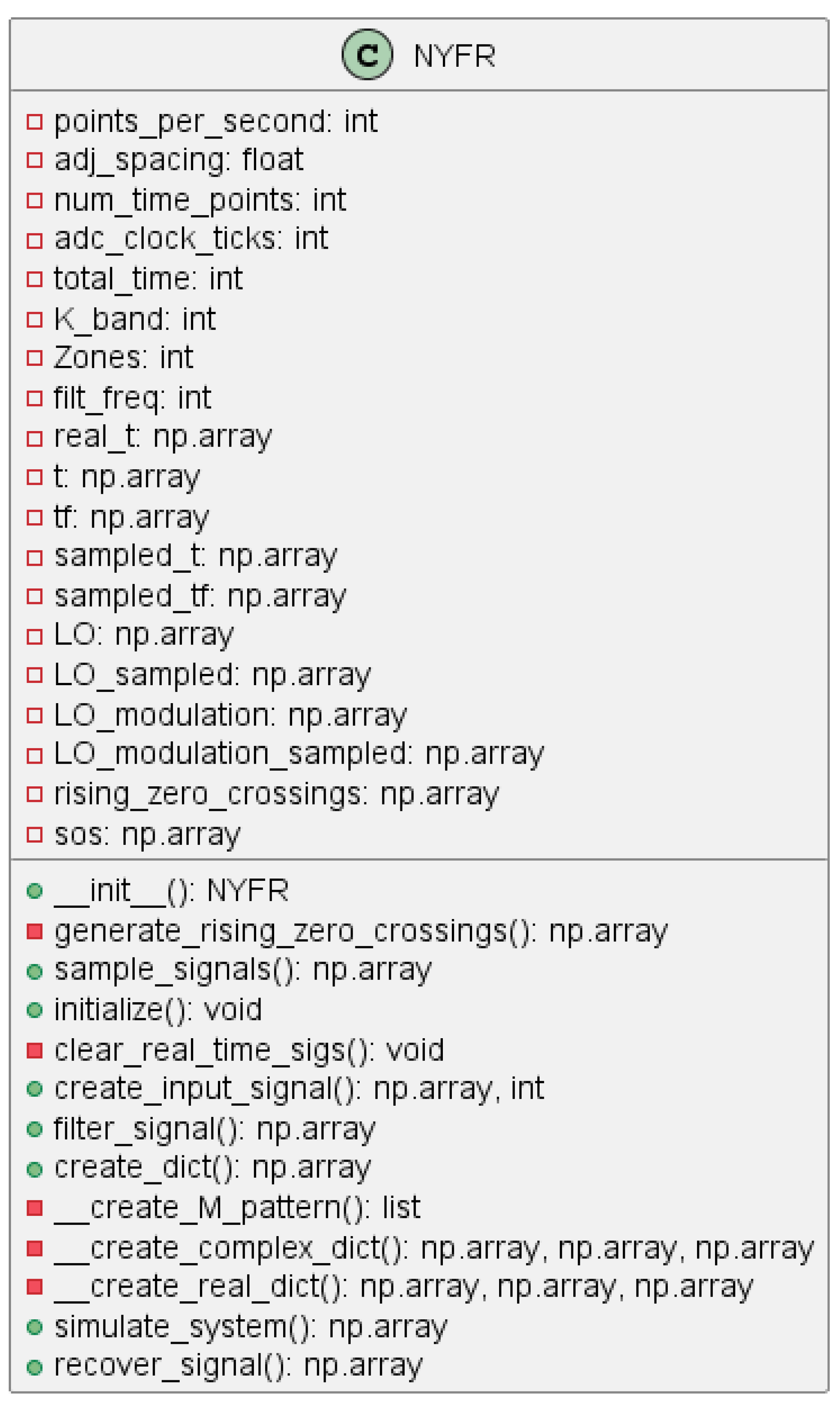
Figure 6.
Nyquist Folding Receiver Sequence Diagram
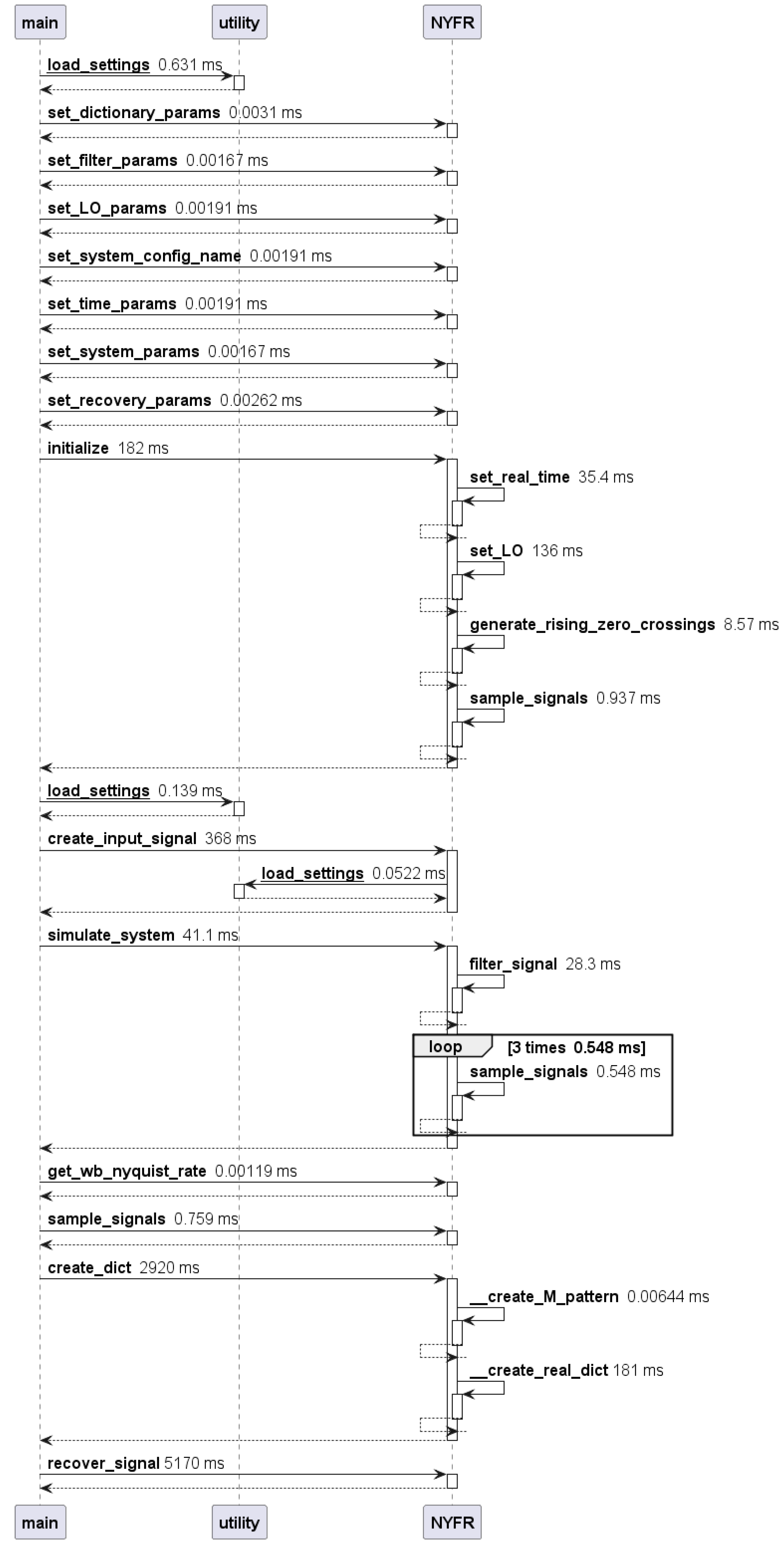
Figure 7.
SpectraMelt MLP with N=4
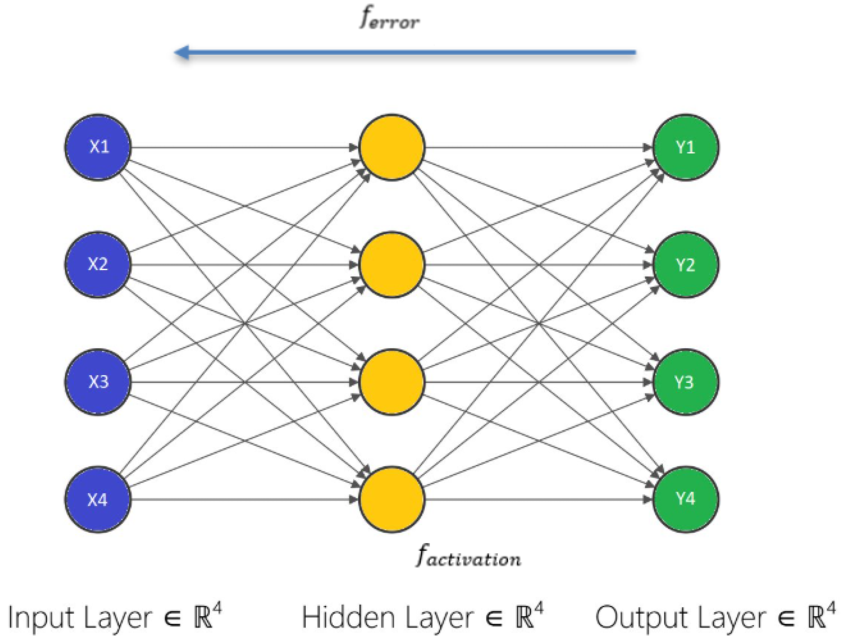
Figure 8.
Initial CS Recovery Guess vs NYFR Outputs: Frequency Domain
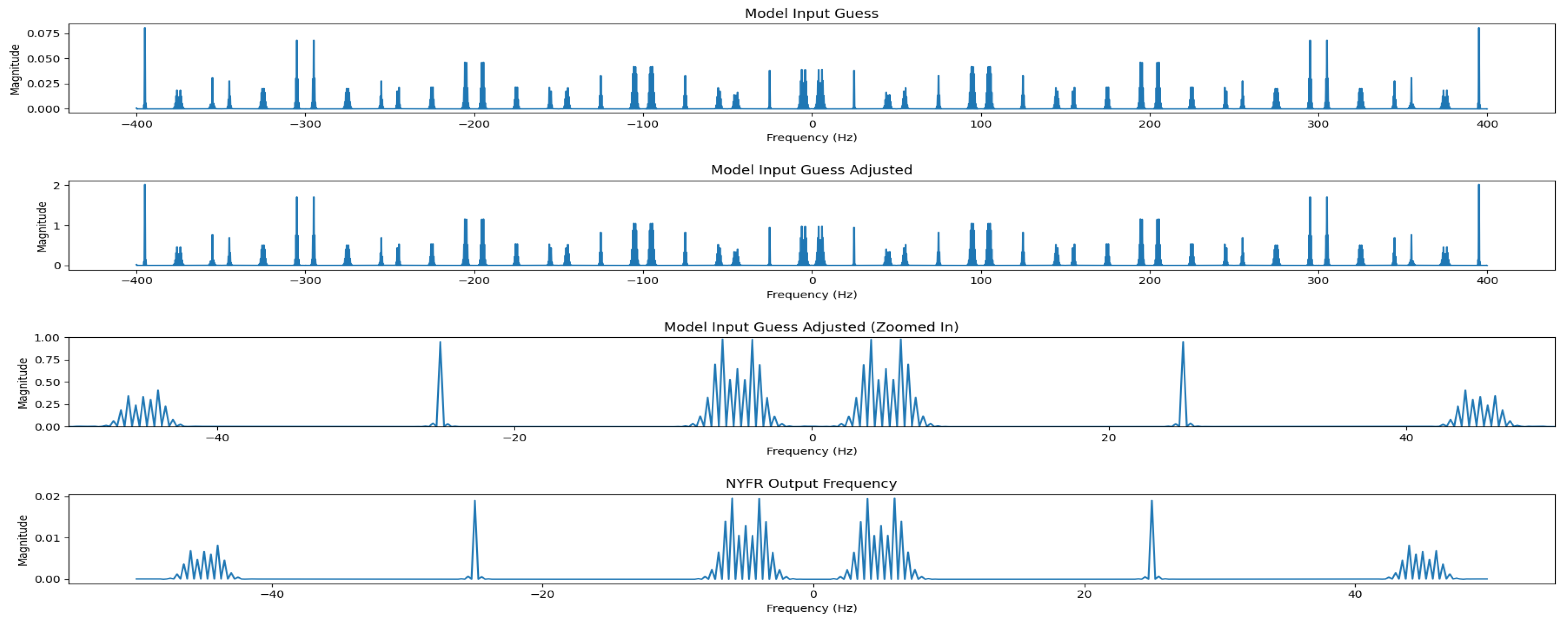
Figure 9.
SpectraMelt Recovered NYFR Outputs: Frequency Domain
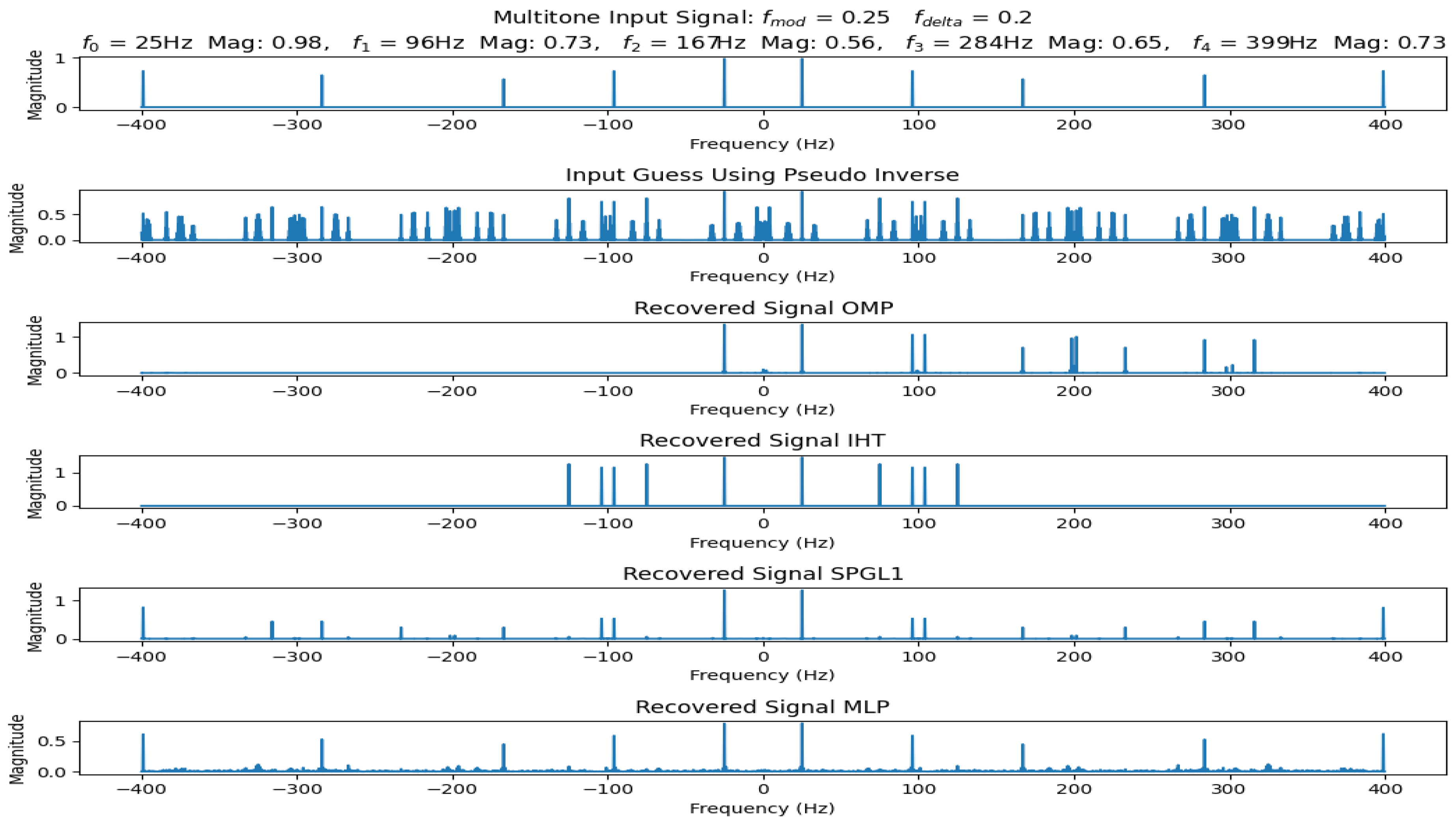

Table 1.
Comparison of recovery methods across different tone counts.
| Tones | Method | Rec. Acc. | Spur Rate | Mag. Err. | Spur Mag. |
|---|---|---|---|---|---|
| 1–2 | IHT | 32.25% | 58.75% | 0.367 | 1.05 |
| 3 | IHT | 32.83% | 65.83% | 1.053 | 1.09 |
| 4 | IHT | 29.63% | 70.38% | 1.685 | 1.17 |
| 5 | IHT | 28.9% | 71.10% | 2.480 | 1.15 |
| 1–2 | OMP | 34.5% | 191% | 0.291 | 52.46 |
| 3 | OMP | 33.17% | 146% | 0.905 | 8124 |
| 4 | OMP | 31.5% | 117% | 1.784 | 131.47 |
| 5 | OMP | 32.3% | 100% | 2.721 | 185.59 |
| 1–2 | SPGL1 | 50% | 129% | 0.574 | 0.825 |
| 3 | SPGL1 | 40.3% | 88.8% | 1.32 | 0.725 |
| 4 | SPGL1 | 33.5% | 58.5% | 2.14 | 0.730 |
| 5 | SPGL1 | 29.4% | 46% | 2.933 | 0.670 |
| 1–2 | MLP | 78.3% | 1% | 0.83 | 0.723 |
| 3 | MLP | 68.7% | 1% | 1.58 | 0.763 |
| 4 | MLP | 56.4% | 1.8% | 2.31 | 0.629 |
| 5 | MLP | 51.9% | 1.1% | 3.11 | 0.660 |
Disclaimer/Publisher’s Note: The statements, opinions and data contained in all publications are solely those of the individual author(s) and contributor(s) and not of MDPI and/or the editor(s). MDPI and/or the editor(s) disclaim responsibility for any injury to people or property resulting from any ideas, methods, instructions or products referred to in the content. |
© 2025 by the authors. Licensee MDPI, Basel, Switzerland. This article is an open access article distributed under the terms and conditions of the Creative Commons Attribution (CC BY) license (http://creativecommons.org/licenses/by/4.0/).
Copyright: This open access article is published under a Creative Commons CC BY 4.0 license, which permit the free download, distribution, and reuse, provided that the author and preprint are cited in any reuse.


