Submitted:
08 October 2025
Posted:
09 October 2025
You are already at the latest version
Abstract
Economic connectedness has been recently found to lower income inequality by rising intergenerational mobility, yet its environmental impacts are less well known. More well-known is the fact that the non-carbon footprint is easier to reach via regulations because its production is domestic. These two problems of income inequality and environmental pollution have echoed in public opinion polls as one of the major current problems in developed countries. We thereby look at the United States on the state level during the last two decades (2010 – 2020) with a Hausman-Taylor estimator for panel data. The choice of the estimator stems from its appropriateness for panel datasets with constant variables. We find that in the United States, economic connectedness between friends, whereby friendships were formed within the same group, may be blamed for the rising environmental (noncarbon) footprint. Noncarbon footprint is, therefore, explained by the bonding of social capital, which may restrict innovation. The policy implications are discussed, and a call is made to distinguish social capital types and promote bridging social capital where bonding social capital is relatively strong.
Keywords:
non-carbon footprint
; economic connectedness
; environment
; social capital
; Hausman-Taylor estimator
1. Introduction
The footprint of grazing land, built-up land, fishing, and forest, namely non-carbon footprint, puts pressure on the environment in the place of production (Aşıcı & Acar, 2018). With increased globalisation, international trade allows more affluent societies to outsource nature-based production in poorer countries through imports, thus enabling them to improve environmental quality at home and meet their ecological footprint empowered by efficient technology and pro-environmental attitudes (Aşıcı & Acar, 2018). Therefore, until the very poor countries have reached income levels that yield environmental improvements and improve environmental conditions worldwide, it is necessary that researchers and policymakers investigate what drives the non-carbon footprint in developed economies and put regulations in place, starting with easier-to-regulate domestic production.
In the United States (US), the environmental footprint due to domestic production has not yet been linked to the economic connectedness (measuring the interaction across class lines), is the form of social capital most strongly associated with economic mobility in developed countries (Chetty et al., 2022) of individuals, and a measure of social capital. With social capital being capable of being built up through public policymaking (Policy Research Initiative (Canada), 2005) and having positive effects as the promotion of socially-minded behaviour and social spillover (Christoforou, 2022), it is worthwhile to study its effects on non-carbon footprint as a tool and determinant of the latter.
Individuals employed in agriculture are not as well-off, not only due to lower wages (U.S. Bureau of Labor Statistics, 2024) but also worse job security (Williams & Horodnic, 2018). Taken together with the fact that low-socioeconomic status individuals are more bound to social communities delined by neighbourhoods (Chetty et al., 2022), researching the social capital effects on non-carbon footprints is also a question of indirectly (through better environmental quality) improving economic and health outcomes, particularly for lower-income individuals, because where one lives matters more for those of low income.
Thus, this investigation takes up a challenge to dissect social capital’s effects on the United States non-carbon footprint over the last two decades using the Hausman-Taylor estimator (see Section 3). Specifically, we ask: is economic connectedness affecting non—carbon footprint, and if so, in which direction? We aim to find out whether economic connectedness has always a positive, environmet-enhancing effect, or may it be also related to lower environmental performance. We find that economic connectedness is likely to raise the non-carbon footprint (see Section 4). Specifically, we have asked whether better economic connectedness leaves us with a less non-carbon footprint. We hypothesise that more social capital in the form of economic connectedness is related to better management of environmental resources and industrial impacts and thus results in a lower non-carbon footprint. However, the results confirm that the opposite may be true. While the symmetrical logic following this result would suggest that segregation of classes would aid in curbing the non-carbon footprint, we offer an alternative explanation (see Section 5 and Section 6 for Discussion and Conclusions, respectively).
This investigation aligns with the work on sustainability planning and scale complexity. Rees (1999) has suggested that humans, as social beings who live in extended groups, overwhelm local ecosystems and need a sense of belonging to the community to bring sustainability. This needs to be done on bioregional levels. Selman (2001) recites the idea of increased social capital as being able to curb losses in eco-capital. However, to this day, these ideas have found little support in the empirical research track.
Therefore, as the main contribution to the literature, we document the case where social capital in the form of economic connectedness may be harmful to the public good, such as the environment. This is yet a less documented implication of social capital effects on environmental-related outcomes. Previously, social capital has been found to promote pro-environmental behaviour and enhance environmental knowledge (Wan & Du, 2022), ease adaptation to climate change (Neil Adger, 2001) and positively impact compliance with both compulsory and economic environmental policy instruments, as well as voluntary measures (Jones et al., 2009).
2. Literature Review
We start by reviewing the past work on this subject to better explain the model we drew up (see Figure 1) and test it in later sections.
Whereas Figure 1 is specific and available data-restricted (further in brackets) in testing how globalisation (exports), the number of people living in the area, disaster resiliency, and industry type (decarbonisation, agriculture) affect economic connectedness, we first review the more abstract theoretical relations from general (social capital) to its specific measurement (economic connectedness) and reference some recent empirical work.
Social capital can be defined as collective assets, such as norms, values, trust, networks and others, that facilitate cooperation and collective action for mutual benefit (Bhandari & Yasunobu, 2009). Generally, two distinct types have been distinguished: bonding and bridging capital. While bridging capital bridges external actors to the focal one, where the focal actor can gain access to others’ resources through new network connections, bonding capital strongly ties the actors with similar backgrounds and interests (Shiu et al., 2024). Economic connectedness, measuring the interaction across class lines, is the form of social capital most strongly associated with economic mobility in developed countries (Chetty et al., 2022), and due to mobility’s positive income inequality outcomes, which are also some of the most salient ones. It can be seen as a bridging form of social capital, because there are bridges built between the high- and low-socioeconomic statuses. As defined by Chetty et al. (2022), economic connectedness is a measure of interaction between individuals and high and low social statuses on social network (Facebook), whereby social status is an index with variables used to predict socio-economic status in a machine learning model being age, city prediction, college attended, county prediction, gender, language, phone model, estimated phone price, mobile carrier and phone operating system type, average donation amount, graduate school attendence, among other variables. Economic connectedness in groups of friendships in which they were made can be understood as a measure of social interaction within the same-origin freindship groupss
What factors (used as the instruments in our benchmark model) impact non-carbon footprint through economic connectedness? Similar at large analyses to ours have found that social capital has a carbon-diminishing effect with the environmental Kuznets curve first rising and then dropping in emissions (Marbuah et al., 2021). No current evidence of carbon emissions affecting social capital exists, but we hypothesise that more developed and emission-heavy environments have low social capital.
The other factor impacting economic connectedness is globalisation. Regarding globalisation and its proxy migration as the indicator, it theoretically affects social capital in both the sending and receiving country, whereby the social capital drops in the receiving developed country (Schiff, 2002). We know that with lower population density, there are higher levels of social capital in the US (Wang & Ganapati, 2018), and there are more resident populations where the population density is low; that is, immigrants are more concentrated in US cities and suburbs (Parker et al., 2018). Thus, one may infer that the social capital levels are higher when there are more resident populations (the rural areas). This is partly approved by Nieminen et al. (2008), who find that although rural and urban region residents do not differ on aggregate, urban areas see less participation and trust than semi-urban and rural regions. The rural regions are also expected to have a higher farm-to-farm production ratio, such that rurality affects social capital.
Regarding disaster resiliency, economic, social, environmental, institutional, infrastructural, and community capital aspects of disaster resilience may univocally impact social capital, and assistance post-disaster has proven to enhance the growth in social capital (Wang & Ganapati, 2018). Generally, disaster community literature states that increases follow consensus crisis shocks in social capital, while corrosive community shocks –are in decline. Still, multiple shocks’ strength and effect are also decisive factors (Besser et al., 2008). We therefore hypothesise that disaster resilience, as a community’s cumulative ability to cope with shocks, should be related to higher social capital in those states.
The more explored causality regarding high-technology exports asks how social capital may affect export growth. However, we wish to shed light on the opposite: how exports (which, along with interstate trade, relate to spatial cluster formation and natural and created comparative advantage) (Wolf, 1997) affect the formation of social capital. We hypothesise that clusters attract immigrant workers because there is a lack of a specialised workforce at home, and thus, with immigration, social capital drops. However, contrary to the individual-level social capital, the firm-level social capital may rise; therefore, on aggregate, social capital is kept at the same level as before the cluster formation. This analysis focuses on individual-level social capital within the state.
Thus, we turn to the question of investigated matter, that is, whether economic connectedness rises, diminishes, or does not impact the non-carbon footprint in a developed country setting. Based on the literature just reviewed, we hypothesise (see Figure 2) that with a higher density of resident population, social capital rises, but at very high levels of population density, it drops, exhibiting an inverse U-curve relationship. This might be because of the fact that in high levels of population density, society becomes highly independent due to the division of work tasks and the short-termism of contacts and social contracts between inhabitants, whereas at very low levels of population density, the linkages between the actors are hard to establish. Therefore, the sign of the population density effect on economic connectedness varies by percentile. Next, the effect of disaster resiliency on social capital is rather positive, as seen in the post-disaster literature. Regarding decarbonisation, we repeat that the hypothesis goes as follows: more developed and emission-heavy environments have low social capital. Regarding the ratio of farm to non-farm labour, the rural regions where there is more farm-to-non-farm labour may see higher participation and trust, as evidenced in the literature. Finally, exports as the proxy for globalisation do not lead to high social capital, as discussed in the previous paragraphs.
Apart from signals just discussed affecting social capital itself, we consider the main question to lay in the linkage between social capital and environmental footprint, more specifically, a non-carbon footprint which is characteristic to the local production activity. We do not make any anterior hypothesis due to the lack of literature on the subject and bring about novel results as an effect. Indeed, there is no previous literature covering the question of social capital and environmental footprint in the highly developed country context.
3. Data and Method
The dataset is composed of variables listed in Table 1 for all states in the United States for the years 2010 and 2020, making it rather cross-sectional.
The variables used in the model aim to reflect the urbanisation rate and economic sophistication of the production, as well as environmental performance as disaster resilience and decarbonisation rate. The ratio of farm to non-farm production relates to non-carbon footprint, as non-carbon footprint is related to place of production, and farming has a strong impact on the enviroenmntal performance. Lastly, foreign-born population aims tp capture the effects of intrenationalisation reflected in the population.
Due to the panel’s short time span, there are only 95 observations (see Table 2). The most dispersed data are found for resident population and farm-to-nonfarm production ratio, whereas the most concentrated variable is disaster resiliency, which signifies largely similar preparedness to disasters in all states.
The steps of the emmpirical approach are depicted in the Figure 3.
The Hausman-Taylor (1981) estimation method was applied to its suitability to the time-invariant variables (in our case, the main regressant EC). It also handles models with unobserved heterogeneity and can be referred to as a regression technique that mixes random and fixed effects. We choose the Hausman-Taylor estimator in place of the other time effect estimators, as autoregressive distributed lag (ARDL) due to its ability to handle EC invariance to time. The Hausman-Taylor estimator was summarised in Ao (2009). It assumed orthogonality between error term and individual effects, that is,
The standard panel data model with time-invariant variables
where covariates X1 , Z1 denote exogenous, and X2 , Z2 endogenous variables and Zi denote time-invariant cross-sectional variables, leaves us with:
and in terms of the particular benchmark model, with:
yit = X’ itβ + Ziγ + µi +ǫit
yit = X’1 itβ1 + X’2 itβ2 + X’3 itβ3 + X’4 itβ4 + X’5 itβ5 + Z1iγ1 + µi +ǫit
NONCARB_FPit = RES_POP’1 itβ1 + DISASTER’2 itβ2 + DECARB’3 itβ3 + HT_EXPORTS’4 itβ4 + FARM_NONFARM’5 itβ5 + EC1iγ1 + µi +ǫit
First, a within transformation is done. All variables in regression are deducted from their group individual mean, and within estimators and residuals are obtained. Then, the residual is regressed on time-invariant variables, using X 1-6 exogenous variables as instruments, and a random effect estimation can be done for each variable. Finally, a Hausman-Taylor estimator is obtained by instrumental variable regression.
We draw up similar OLS, FE and RE models to supplement the Hausman-Taylor benchmark model. Different instruments are utilised for Hausman-Taylor estimation, as shown in Eq. 4, with the respective results in Table 4.
NONCARB_FPit = RES_POP’1 itβ1+ DISASTER’2 itβ2+ DECARB’3 itβ3+ HT_EXPORTS’4 itβ4+ FOREIGN’5 itβ5+ EC1iγ1+ µi +ǫit
Lastly, the assumptions of the absence of collinearity (Belsley, 1991), exogeneity for the EC variable (Hausman, 1978), and homoskedasticity (Breusch & Pagan, 1979) are tested. The Hansen-Sargan test is applied to test for instrument validity (Sargan, 1958).
4. Empirical Results
Before estimating the benchmark model, we draw up a matrix of correlations, test for multicollinearity with VIF and test for cross-sectional dependence. We depict the results in Table 3 below.

Table 3.
Pre-test results.
| Test name | Statistics / variables | |||
| Exogeneity test (Hausman) | Chi2 | Df | p-value | |
| 14.852 | 4 | 0.0050 | ||
| Multicollinearity (VIF) test | EC | FARM_NONFARM | NASICI | RES_POP |
| 1.2663 | 1.1757 | 1.5859 | 1.5895 | |
| Homoeskedasticity test (Breausch–Pagan) | BP | Df | p-value | |
| 5.2747 | 4 | 0.2603 | ||
Notes: H0 for the Hausman test is that random effects are at work; this hypothesis is rejected in favour of fixed effects. VIF values are usually deemed to be high if the value is higher than 8. H0 for Breuasch–Pagan test is the presence of heteroskedasticity.
Table 4.
Estimation results for instrumental variables of Eq. 3.
| Dependent: NONCARB_FP | Hausman-Taylor | OLS | FE | RE |
| Time-varying exogenous | ||||
| RESID_POP | -0.0350*** | -0.0314*** | -0.0334*** | |
| DISASTER | ||||
| FARM_NONFARM | -0.0034 | -0.0078 | -0.0053 | |
| DECARB | ||||
| HT_EXPORTS | ||||
| FOREIGN | - | |||
| NASICI | - | 0.1639*** | 0.1474*** | 0.1564*** |
| Time-invariant endogenous | ||||
| EC | 0.5489*** | 0.4517*** | 0.4245*** | 0.4406*** |
| Constant | 1.8094*** | 1.6723*** | 1.6676*** | |
| Number of observations | 95 | 95 | 95 | 95 |
| Total sum of squares | 0.8537 | 0.7750 | 0.9221 | |
| Residual sum of squares | 0.3137 | 0.2279 | 0.2563 | |
| R-squared | 0.6334 | 0.7105 | 0.7060 | 0.7222 |
| Adjusted R-squared | 0.6294 | 0.6976 | 0.6670 | 0.7099 |
| F-statistic | - | 55.22*** | 49.821*** | |
| Wald chi-square | 100.321*** | 217.612*** | ||
| Hansen-Sargan test | 0.4107*** | |||
Note: All variables enter regressions in logs and are winsorised to the upper and lower 10%. The R function " PLM" was used to obtain results for Hausman-Taylor and FE, RE estimation, and "lm" to obtain OLS estimates.
Next, we present the matrix of correlations between the variables that enter the Hausman-Taylor estimation, presented in Figure 3. Although the correlation between some variables, such as EC and NONCARB_FP, is quite high, we reinforce the idea that the two are highly different in nature and come from different sources with different natures.
We first estimate the benchmark model via the Hausman-Taylor estimator (instrumented by resident population, disaster resiliency, farm-to-nonfarm production, decarbonisation and high-technology exports). Then, similar models involving the NASICI competitiveness index are tested via OLS, FE and RE, as can be seen in Table 3. NASICI variable is included only in the other than benchmark models because it is not likely to impact economic connectedness instrumentally. The other regressions are supplemented by variables which previously entered Hasuman-Taylor estimation as instruments, namely, resident population and farm-to-nonfarm production. The choice of not using all instruments as independent variables is due to the significance of the data-tested modelling, not as much due to the conceptual and theoretical considerations. However, we hold that farm-to-nonfarm production should directly impact the footprint from non-carbon emissions and, therefore, include it in OLS, FE and RE models.
Estimation results in Table 4 (see Eq. 3) show that economic connectedness (EC) strongly predicts a noncarbon footprint (NONCARB_FP). The noncarbon footprint rises with a smaller resident population (RESID_POP) and a higher competitiveness index (NASICI). While the farm-nonfarm production ratio (FARM_NONFARM) is a valid instrument for economic connectedness, it is not a strong enough predictor of noncarbon footprint. Because all the econometric estimations follow the same pattern, we declare the benchmark estimation to be robust. Next, we turn to estimations for robustness with different sets of instruments (see Eq. 4) focusing on globalisation and thus involving foreign-born population and competitiveness, but not farm-nonfarm production.
In Table 5, one can again notice that the general effects of economic connectedness (EC) on noncarbon footprint (NONCARB_FP) remain the same, but the effect is slightly larger in the case where we instrument for globalisation (FOREIGN). The resident population (RESID_POP) seems to have reduced its footprint, while more competitive industries (NASICI) in the state have raised it. These three main results remain largely intact.
We have tested our results after regressions (see Table 6).
The Hansen-Sargan tests (Sargan, 1958) validity of the instrument choice, the shallow variance inflation factor values allow us to assume there is a lack of collinearity (Belsley, 1991). Durbin-Wu-Hausman (Hausman, 1978) tests allow us to conclude that the RE alternative is the consistent estimator, and the Breusch-Pagan test (Breusch & Pagan, 1979) establishes that the variance of the errors from regression is dependent on the values of independent variables; that is, there is no significant homoskedasticity.
5. Discussion and Implications for Policy
The principal model of economic connectedness in groups of friendships in which they were made, bringing about a higher non-carbon ecological footprint, could be explained by the narrative of two existing research streams with respective results: rigid social networks and information technology use.
Rigid Social Networks
First, friendships that can be allocated to the group they were formed suggest that individuals in question do not generally reallocate and maintain friendships within the same groups. This is because the further one lives, the less likely one is to form friendships with someone of different age and race (Nahemow & Lawton, 1975).
This suggests a rigid social network, where the more closely tied structures bring about constrained social behaviour and less innovation (Burt, 2000). If this is the case and social capital is of bonding (opposite of bridging as distinguished in (Iantosca et al., 2024) type, which is likely in the case of same-group social connectedness, as it is easier to maintain in the long-term (van Cleemput, 2012), then friendships made and maintained in the same groups are less likely to bring about (economic and social) innovation. Less innovation is, in turn, related to more primary-sector-oriented economic activities where less technology is applied. This is due to the general finding in developed countries that patents (innovativeness) and value-added are generally positively correlated (Schmoch et al., 2003), at the same time, abstaining from claiming industries to represent homogeneous technologies.
Information Technology Use
Another explanation of friendships maintained in the same group in which they were formed might be related to better and more widely used information technology and online social networks. While physical distance matters despite the internet, relationship persistence has changed. Nevertheless, most networks in the US are within driving distance (Holmes, 2012).
The other minor findings from complementary models indicate that the amount of resident population and economy being knowledge-based, globalised and innovation-ready takes a front seat in determining the non-carbon footprint outcome. While the resident population has a footprint-relieving effect, we find that overall competitiveness raises footprint. This dynamic ties well with our previous observation that bonding social capital-driven states is less innovative, productive, and, therefore, less polluting. At the same time, competitiveness brings about a larger non-carbon footprint.
The policy implications of these findings, abiding still by the general result found in the literature of social capital generally bringing a positive impact on emission reduction or doing so in a Kuznets way, may imply that we need to find new ways how to inject bridging social capital in states and communities where social capital of bonding type is prevalent and strong. This is to be done in order to revive innovation in closely tied groups, which may otherwise abide by know-how already embedded into the industry in which production takes place. This improvement could potentially bring new innovation from individuals of other income levels and, likely also, economic migrants, who may otherwise choose to in-migrate into states with lower resident populations where the bridging social capital is already high (that is, they have an easier time to develop bridges to climb the income ladder).
Although community action is predicted by bridging and bonding social capital, one form can compensate for weaknesses in the other (Agnitsch et al., 2006). We find that the bonding social capital undermines environmental outcomes and calls for careful actions that set bridging capital to emerging, as bonding capital may be hampered on the way(Leonard, 2004). Dispersed social housing programs, school class composition programs, and other actions aiming at closer interactions across socio-economic levels for individuals and families of all ages and races can inject bridging social capital in places with high bonding capital.
However, caution must be taken when interpreting the findings very strongly, as the research suffers from scarce data availability, drawing on a rather small set of observations available for two decades (2010 and 2020). We nevertheless maintain that the key relationship between social capital and environmental footprint may not always be positive, as shown in this investigation.
6. Conclusions
We have established a possible interconnection between social capital and environmental footprint, and we now call for further exploration of the mechanisms at work.
The hypothesis of social capital having a positive effect on environmental footprint is not approved, only to find out that bonding social capital may be, in fact, negatively related to non-carbon footprint. This finding is supplemented with the fact that a higher resident population diminishes footprint, while the higher competitiveness of the state increases it. They are relevant to the discussion on social capital-enhancing policies as the tool for collective, environmentally-conscious action resulting in better environmental outcomes. Significantly, we may not always reach positive environmental outcomes when promoting bonding social capital. Therefore, distinguishing between social capital at all levels of policymaking is advised. That said, bonding social capital – social capital that is based on networks that are close-knit, continuous and strong, may be harmful. To reach the benefits of high social capital, one may want to focus on bridging social capital, which characterises weaker ties applied across broad social networks. Such ties can be developed in large community groups, such as larger voluntary groups and broader school classes and mingling activities in after-school interest education groups, to give a few examples for all age groups.
As for limitations of the study, these findings establish a research avenue and demand more inquiry with other developed country datasets or, when available, a longer time span inquiry in the United States. Indeed, the time span considered in this study does not allow for a high-precision study of changes in social capital and their effects on noncarbon footprint. Neither does the limited number of cross-sections allow us to draw broader conclusions that would apply to developed countries in general.
As for future research proposects, in the future, therefore, upon the development of social capital measures for other developed countries, one may want to study other areas where economies and societies are highly developed. Moreover, one may want to track developments of social capital, natural resources and environmental footprints in particular through the centuries, to reach better insights into the modes of operation of these two variables in relation one to another.
References
- Agnitsch, K., Flora, J., & Ryan, V. (2006). Bonding and Bridging Social Capital: The Interactive Effects on Community Action. Community Development, 37(1), 36–51. [CrossRef]
- Ao, X. (2009). An introduction to Hausman-Taylor model 1 Hausman-Taylor model.
- Aşıcı, A. A., & Acar, S. (2018). How does environmental regulation affect production location of non-carbon ecological footprint? Journal of Cleaner Production, 178, 927–936. [CrossRef]
- Belsley, D. A. (1991). A Guide to using the collinearity diagnostics. Computer Science in Economics and Management, 4(1), 33–50. [CrossRef]
- Besser, T. L., Recker, N., & Agnitsch, K. (2008). The Impact of Economic Shocks on Quality of Life and Social Capital in Small Towns*. Rural Sociology, 73(4), 580–604. [CrossRef]
- Bhandari, H., & Yasunobu, K. (2009). What is Social Capital? A Comprehensive Review of the Concept. Asian Journal of Social Science, 37(3), 480–510. [CrossRef]
- Breusch, T. S., & Pagan, A. R. (1979). A Simple Test for Heteroscedasticity and Random Coefficient Variation. Econometrica, 47(5), 1287. [CrossRef]
- Burt, R. S. (2000). The Network Structure of Social Capital. In Research in organizational behavior : an annual series of analytical essays and critical reviews (p. 292). JAI.
- Chetty, R. (2022). Data library. OpportunityInsights. https://opportunityinsights.org/data/.
- Chetty, R., Jackson, M. O., Kuchler, T., Stroebel, J., Hendren, N., Fluegge, R. B., Gong, S., Gonzalez, F., Grondin, A., Jacob, M., Johnston, D., Koenen, M., Laguna-Muggenburg, E., Mudekereza, F., Rutter, T., Thor, N., Townsend, W., Zhang, R., Bailey, M., … Wernerfelt, N. (2022). Social capital II: determinants of economic connectedness. Nature, 608(7921), 122–134. [CrossRef]
- Christoforou, A. (2022). Social Capital and Civil Society in Public Policy, Social Change, and Welfare. Journal of Economic Issues, 56(2), 326–334. [CrossRef]
- Global Footprint Network. (2023). Public Data Package. https://www.footprintnetwork.org/licenses/public-data-package-free/.
- Hausman, J. A. (1978). Specification Tests in Econometrics. Econometrica, 46(6), 1251. [CrossRef]
- Hausman, J. A., & Taylor, W. E. (1981). Panel Data and Unobservable Individual Effects. Econometrica, 49(6), 1377. [CrossRef]
- Holmes, K. (2012). Perceived Difficulty of Friendship Maintenance Online: Geographic Factors. Advances in Applied Sociology, 02(04), 309–312. [CrossRef]
- Iantosca, M. H., Kimelberg, S. M., Lewis, D. V., & Taughrin, R. J. (2024). “We’re gonna get you through it”: The role of bonding social capital in the development of bridging social capital. Sociological Forum, 39(1), 22–34. [CrossRef]
- ITIF. (2022). North American Subnational Innovation Competitiveness Index. https://itif.org/publications/2022/06/21/north-american-subnational-innovation-competitiveness-index/.
- Jones, N., Sophoulis, C. M., Iosifides, T., Botetzagias, I., & Evangelinos, K. (2009). The influence of social capital on environmental policy instruments. Environmental Politics, 18(4), 595–611. [CrossRef]
- Leonard, M. (2004). Bonding and Bridging Social Capital: Reflections from Belfast. Sociology, 38(5), 927–944. [CrossRef]
- Marbuah, G., Gren, I.-M., & Tirkaso, W. T. (2021). Social capital, economic development and carbon emissions: Empirical evidence from counties in Sweden. Renewable and Sustainable Energy Reviews, 152, 111691. [CrossRef]
- Nahemow, L., & Lawton, M. P. (1975). Similarity and propinquity in friendship formation. Journal of Personality and Social Psychology, 32(2), 205–213. [CrossRef]
- Neil Adger, W. (2001). Social Capital and Climate Change.
- Nieminen, T., Martelin, T., Koskinen, S., Simpura, J., Alanen, E., Härkänen, T., & Aromaa, A. (2008). Measurement and socio-demographic variation of social capital in a large population-based survey. Social Indicators Research, 85(3), 405–423. [CrossRef]
- Parker, K., Horowitz, J., Brown, A., Fry, R., Cohn, V., & Igielnik, R. (2018). What Unites and Divides Urban, Suburban and Rural Communities (Vol. 22). www.pewresearch.org.
- Policy Research Initiative (Canada). (2005). Social capital as a public policy tool : project report. Policy Research Initiative.
- Rees, W. (1999). Scale, complexity and the condundrum of sustainability. In Planning Sustainability (pp. 101–127).
- Sargan, J. D. (1958). The Estimation of Economic Relationships using Instrumental Variables. Econometrica, 26(3), 393. [CrossRef]
- Schiff, M. (2002). Love thy neighbor: Trade, migration, and social capital. European Journal of Political Economy, 18(1), 87–107. [CrossRef]
- Schmoch, U., Laville, F., Patel, P., & Frietsch, R. (2003). Linking Technology Areas to Industrial Sectors Final Report to the European Commission, DG Research.
- Selman, P. (2001). Social capital, sustainability and environmental planning. Planning Theory and Practice, 2(1), 13–30. [CrossRef]
- Shiu, J.-M., Dallas, M. P., & Lin, P.-H. (2024). Collaboration and social capital in meta-organisations: bonding or bridging? Technology Analysis & Strategic Management, 1–13. [CrossRef]
- Stats America. (n.d.). Downloads. Retrieved 11 September 2024, from https://www.statsamerica.org/downloads/default.aspx.
- Bureau of Labor Statistics. (2024, July). Employment and average hourly earnings by industry. https://www.bls.gov/charts/employment-situation/employment-and-average-hourly-earnings-by-industry-bubble.htm.
- US Census Bureau. (n.d.). Data. Retrieved 11 September 2024, from https://www.census.gov/data/tables/time-series/dec/density-data-text.html.
- van Cleemput, K. (2012). FRIENDSHIP TYPE, CLIQUE FORMATION AND THE EVERYDAY USE OF COMMUNICATION TECHNOLOGIES IN A PEER GROUP: A social network analysis. Information Communication and Society, 15(8), 1258–1277. [CrossRef]
- Wan, Q., & Du, W. (2022). Social Capital, Environmental Knowledge, and Pro-Environmental Behavior. International Journal of Environmental Research and Public Health, 19(3), 1443. [CrossRef]
- Wang, L., & Ganapati, N. E. (2018). Disasters and Social Capital: Exploring the Impact of Hurricane Katrina on Gulf Coast Counties. Social Science Quarterly, 99(1), 296–312. [CrossRef]
- Williams, C. C., & Horodnic, A. V. (2018). Tackling Undeclared Work in the Agricultural Sector. https://www.researchgate.net/publication/328997230.
Figure 1.
Instrumental variable model of noncarbon footprint. Note: RES_POP denotes resident population; DISASTER denotes disaster resiliency; DECARB denotes decarbonisation; FARM_NONFARM denotes farm-to-nonfarm production ratio; EXPORTS denote high-technology exports; EC denotes economic connectedness; NONCARB_FP denotes non-carbon footprint.
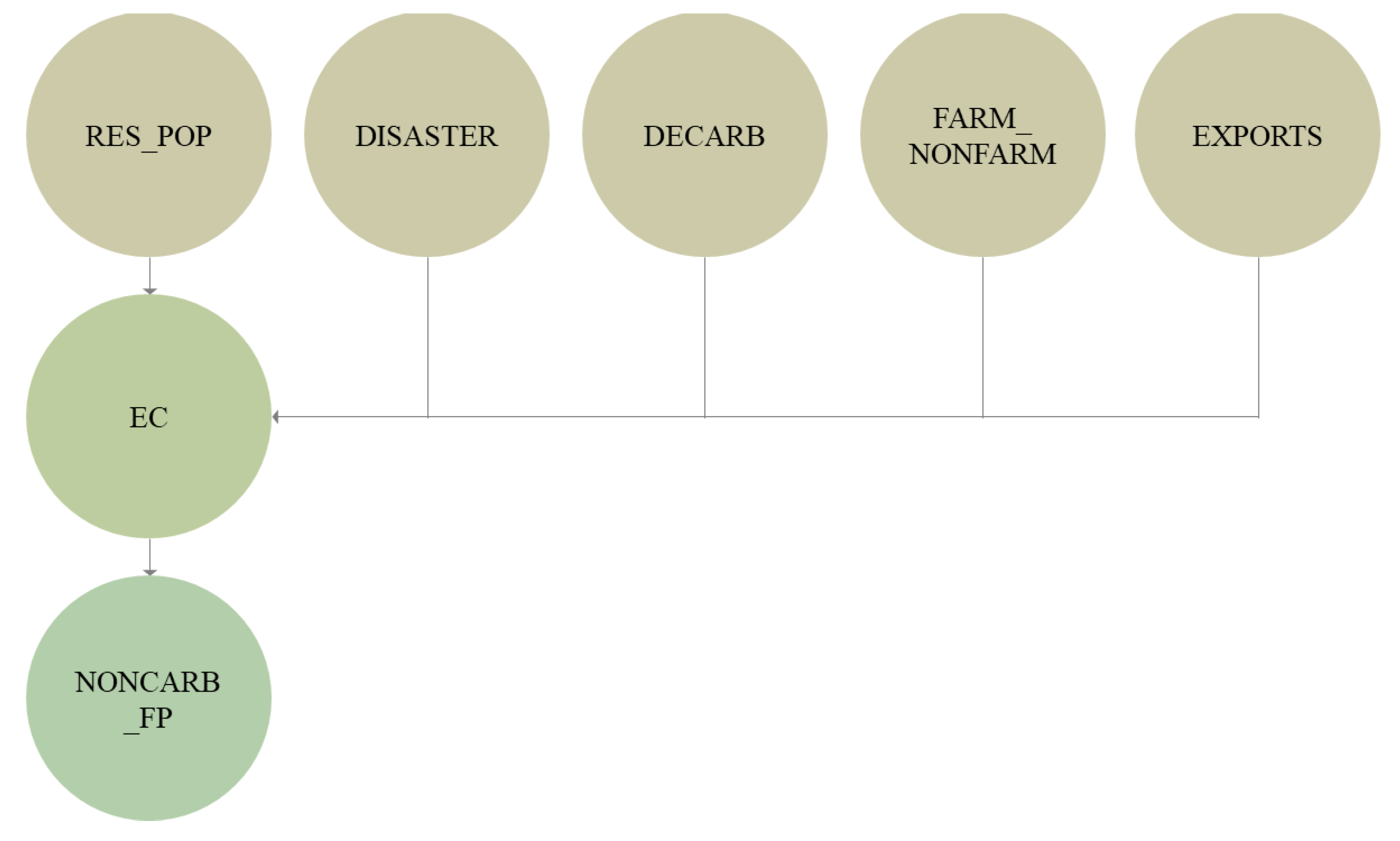
Figure 2.
Conceptual framework.
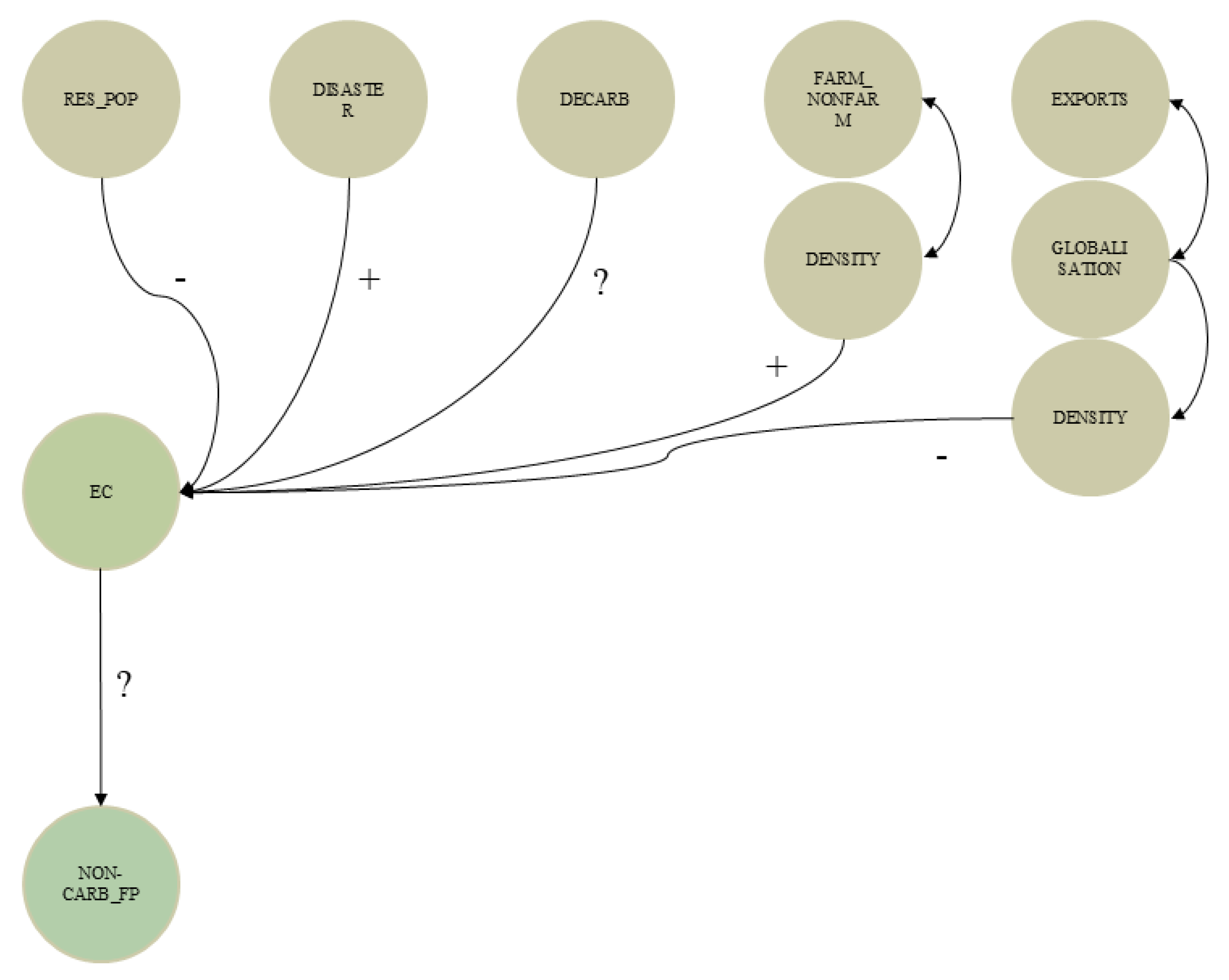
Figure 3.
The empirical approach of the investigation.
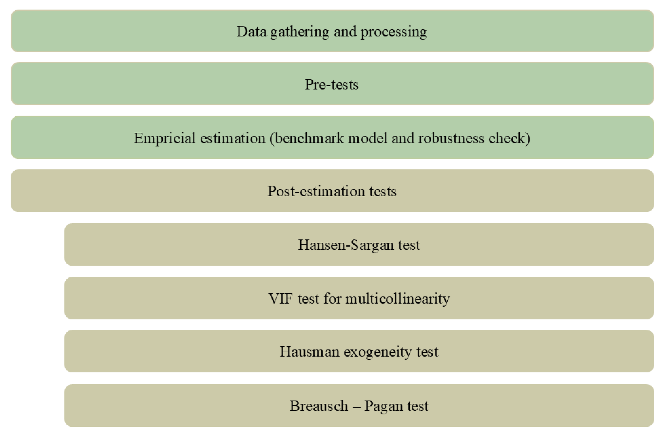
Figure 3.
Correlation matrix. Source: authors’ calculations.
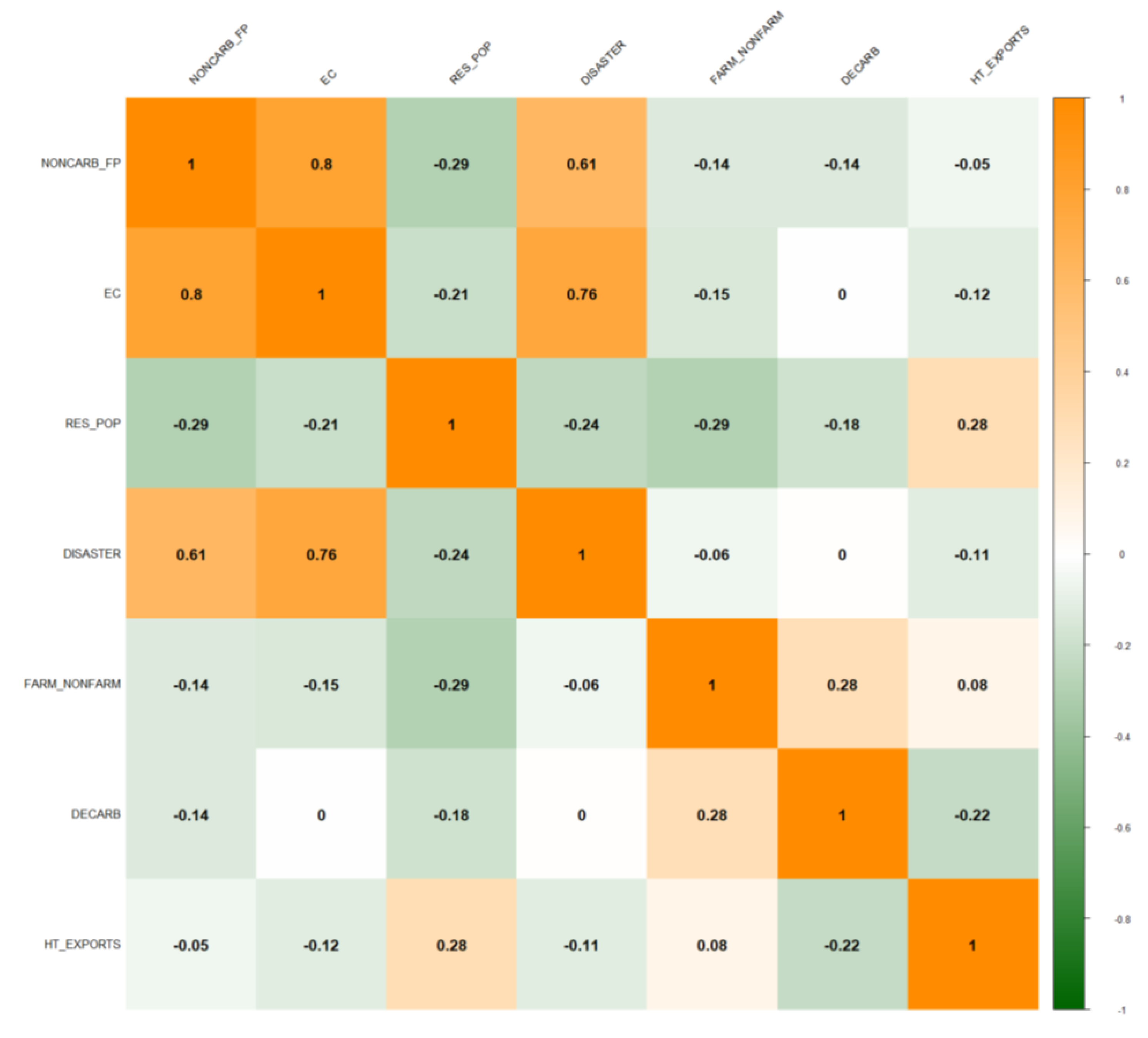
Table 1.
Data description and sources.
| Variable | Full Name | Source |
|---|---|---|
| NONCARB_FP | Non-carbon footprint | Global Footprint Network (2023) |
| RES_POP | Resident population | US Census Bureau (n.d.) |
| DISASTER | Disaster resilience | Stats America (n.d.) |
| DECARB | Decarbonisation | ITIF (2022) |
| HT_EXPORTS | High-tech exports | ITIF (2022) |
| FARM_NONFARM | The ratio of farm to non-farm production | Stats America (n.d.) |
| FOREIGN | Foreign-born population | US Census Bureau (n.d.) |
| EC | Economic connectedness within group membership | Chetty (2022) |
Note: All variables were readily taken by state, and no transformations from levels of aggregation were made.
Table 2.
Descriptive Statistics.
| Variable | Obs. | Min | Max | Mean | S-D |
|---|---|---|---|---|---|
| NONCARB_FP | 95 | 1.649 | 1.943 | 1.788 | 0.1012 |
| RES_POP | 95 | 13.700 | 16.370 | 15.190 | 0.8830 |
| DISASTER | 95 | -0.840 | -0.584 | -0.702 | 0.0887 |
| DECARB | 95 | 2.504 | 3.387 | 2.892 | 0.2849 |
| HT_EXPORTS | 95 | -4.999 | -3.533 | -4.228 | 0.5121 |
| FARM_NONFARM | 95 | -6.974 | -3.361 | -5.111 | 1.0903 |
| FOREIGN | 95 | -3.409 | -1.702 | -2.616 | 0.5785 |
| EC | 95 | -0.3041 | 0.1479 | -0.0395 | 0.1481 |
Note: All variables are in logs and winsorised by upper and lower 10%. Obs. and S-D denote the number of observations and standard deviation, respectively.
Table 5.
Estimation results for instrumental variables of Eq. 4.
| Dependent: NONCARB_FP | Hausman-Taylor | OLS | FE | RE |
| Time-varying exogenous | ||||
| RESID_POP | -0.0351*** | -0.0312*** | -0.0342*** | |
| DISASTER | ||||
| FARM_NONFARM | - | |||
| DECARB | ||||
| HT_EXPORTS | ||||
| FOREIGN | 0.0072 | 0.0111 | 0.0078 | |
| NASICI | - | 0.1546** | 0.1384** | 0.1512** |
| Time-invariant endogenous | ||||
| EC | 0.5718*** | 0.4514*** | 0.4242*** | 0.4463*** |
| Constant | 1.8103*** | 1.7467*** | 1.7450*** | |
| Number of observations | 95 | 95 | 95 | 95 |
| Total sum of squares | 0.8579 | 0.7750 | 0.9489 | |
| Residual sum of squares | 0.3178 | 0.2318 | 0.2682 | |
| R-squared | 0.6335 | 0.7102 | 0.7009 | 0.7174 |
| Adjusted R-squared | 0.6296 | 0.6973 | 0.6613 | 0.7049 |
| F-statistic | 55.14*** | 48.6281*** | ||
| Wald chi-square | 137.937*** | 217.988*** | ||
Note: All variables enter regressions in logs and are winsorised to the upper and lower 10%. The R function " PLM" was used to obtain results for Hausman-Taylor and FE, RE estimation, and "lm" to obtain OLS estimates.
Table 6.
Post-estimation tests.
| Eq. 3 (Table 3) | Hausman-Taylor | OLS | FE | RE |
| Hansen-Sargan test | 0.4107*** | |||
| VIF (max value) | 1.5895 | |||
| Hausman exogeneity test | 27.731*** | |||
| Breusch-Pagan test | 5.2747 | |||
| Eq. 4 (Table 4) | ||||
| Hansen-Sargan test | 1.9028*** | |||
| VIF (max value) | 2.2822 | |||
| Hausman exogeneity test | 24.344*** | |||
| Breusch-Pagan test | 5.5672 |
Disclaimer/Publisher’s Note: The statements, opinions and data contained in all publications are solely those of the individual author(s) and contributor(s) and not of MDPI and/or the editor(s). MDPI and/or the editor(s) disclaim responsibility for any injury to people or property resulting from any ideas, methods, instructions or products referred to in the content. |
© 2025 by the authors. Licensee MDPI, Basel, Switzerland. This article is an open access article distributed under the terms and conditions of the Creative Commons Attribution (CC BY) license (http://creativecommons.org/licenses/by/4.0/).
Copyright: This open access article is published under a Creative Commons CC BY 4.0 license, which permit the free download, distribution, and reuse, provided that the author and preprint are cited in any reuse.


