
Submitted:
07 October 2025
Posted:
08 October 2025
You are already at the latest version
Abstract
Time series analysis is of critical importance in a wide range of applications, including weather forecasting, anomaly detection, and action recognition. Accurate time series forecasting requires modeling complex temporal dependencies, particularly multi-scale periodic patterns. To address this challenge, we propose a novel Wavelet-Enhanced Transformer (Wave-Net). Wave-Net transforms 1D time series data into 2D matrices based on periodicity, enhancing the capture of temporal patterns through convolutional filters. This paper introduces Wave-Net, a model that incorporates wavelet and Fourier transforms for feature extraction, along with an enhanced cycle offset and optimized dynamic K for improved robustness. The Transformer layer is further refined to bolster long-term modeling capabilities. Evaluations on real-world benchmarks demonstrate that Wave-Net consistently achieves state-of-the-art performance across mainstream time series analysis tasks.
Keywords:
Wave-Net
; wavelet transform
; Fourier transform
; dynamic K selection
; the Transformer layer
1. Introduction
Time series analysis is of immense importance in extensive applications and action recognition. Such applications include forecasting meteorological factors for weather prediction [1]; detecting anomalies in monitoring data for industrial maintenance [2]; imputing missing data for data analysis [3]; and classifying trajectories for action recognition [4]. Time series analysis has received great interest owing to its immense practical value [5]. Time series are continuous records that only save some scalars at each time point, unlike other types of sequential data, such as language, images, and videos. Typically, a single time point does not provide enough semantic information. Therefore, many studies focus on changes over time, which contain more information and can reflect the intrinsic properties of time series, such as continuity, periodicity, and trends. However, changes in time series in the real world are always complex. They involve multiple changes, such as increases, decreases, and fluctuations that mix and overlap. This makes time change modeling extremely challenging, especially when it comes to accurately measuring and analyzing the effects of time change on various systems and processes. In the domain of deep learning, the advanced nonlinear modeling capabilities of deep models have led to the development of numerous methods that researchers have employed to capture the intricate dynamic properties of real-world time series. Early approaches primarily employed recurrent neural networks (RNNs) to model time-series dependencies based on Markov assumptions[6] [7]. However, RNN-like models face challenges in effectively capturing long-term dependencies and are constrained by the limitations of sequential computation. Another class of approaches utilizes temporal convolutional networks (TCNs) to extract local patterns [8][9]. However, the locally-aware nature of their one-dimensional convolutional kernel leads to limited long-term dependency modeling capabilities. In recent years, Transformer-based architectures have achieved significant advances in sequence modeling through the utilization of the global attention mechanism [9]. In the domain of time series analysis, researchers have enhanced the attention mechanism to capture global dependencies.
As demonstrated in the studies conducted by Zhou et al. [10] and Liu et al. [11], sparse aattention variants serve to reduce computational complexity. Attention mechanisms operating within the frequency domain [12] [13] have been shown to enhance the capture of periodic patterns. Hierarchical temporal modeling is a methodology used to disassociate intricate temporal patterns.
However, given that temporal dependencies frequently become obscured by noise and multiscale patterns present in real-world scenes, standard attentional mechanisms often encounter difficulties in reliably recognizing deep dependencies directly from the original time points[14].
We observe that real-world time series typically exhibit multiple periodicities, such as daily and annual variations in weather observations, as well as fixed-interval traffic flow prediction. These multiple periods overlap and interact with each other. We refer to these two types of time variation as intra-period variation and inter-period variation, respectively. The former denotes short-term temporal patterns within cycles, while the latter reflects long-term trends over successive periods. For time series without a clear periodicity, the variation will be dominated by inter-period variation. To tackle the intricacies of time variation, we analyze the time series in a new dimension of multi-periodicity.
Based on the motivation above, the multi-periodicity of time series is discovered, and the corresponding time-varying modular architecture is captured. Specifically, intra-periodic and inter-periodic variations in 2D space can be further captured by parameter-efficient residual blocks adaptively. This study aims to address the challenges in adaptive multi-period time series forecasting by proposing a Wavelet-Enhanced Transformer (Wave-Net) framework. The development of Wave-Net is inspired by the superior performance of the TimesNet architecture [15]. Our contribution summarizes three aspects:
1. Combine the wavelet transform and the Fourier transform for feature extraction, and enhance the cycle offset.
2. The hyperparameter K (number of cycles selected) is dynamically learnable and not just based on the amplitude of selecting the first K cycles.
3. Use a Transformer layer to further improve model performance on complex time series forecasting or analysis tasks, enhancing the ability to capture long-term dependencies and complex patterns.
2. Related Work
Time-varying modeling has been well explored in the field of time series as a key issue in time series analysis. Many traditional methods have been proposed, such as the Box-Jenkins method [16], structural decomposition models (e.g., STL [17] ), and financial volatility frameworks (e.g., GARCH [18] ). However, the complexity displayed by real-world time series limits their utility in dynamic applications.
In recent years, deep learning methods for time series modeling have emerged, mainly including representative models based on MLP, TCN, and RNN. MLP-based methods apply a multilayer perceptron in the time dimension and solidify temporal dependencies in the fixed weight parameters of the MLP layer. The TCN-based approach utilizes a convolutional kernel that slides along the time dimension to capture temporal patterns in the sequence. RNN-based approaches implicitly model the dynamics of the sequence by passing hidden states between time steps through a recursive structure. However, these classical paradigms, while effective, fail to explicitly model and exploit the periodicity-driven changes in the two-dimensional time structure proposed in this paper.
In addition, to deal with complex temporal patterns, Autoformer[1] also proposed a deep decomposition architecture to obtain the seasonal and trend portions of the input series. Later, FEDformer [19] employs an expert hybrid design to enhance the seasonal trend decomposition and presents sparse attention in the frequency domain. Unlike the previous single-period extraction methods, we unravel the intricate temporal patterns by introducing wavelet transform and the Fourier transform for time-frequency conversion, exploring the multi-periodicity of the time series, dynamically adjusting the learnable K-values to optimize the model performance, and finally utilizing the self-attention mechanism to capture the intricate and dynamic long-term dependencies and global patterns spanning the entire length of the series and to incorporate the multiscale information.
3. Methodology
Given a time series X containing D variables or channels, the goal of time series forecasting is to predict the next H future steps based on past observations of length L, mathematically represented as follows:
denotes the data series from time to time t, which is the matrix of past observations with the shape of . denotes the data series from time to time , which is the matrix of future predicted values with the shape of . The inherent periodicity in the time series is the basis for accurate forecasting, especially when predicting over large horizons such as 96–720 steps (equivalent to days or months). To improve model performance in long-term prediction tasks, we propose a new model. The proposed method combines the wavelet transform and the Fourier transform to form a simple yet powerful approach.
3.1. The Wavelet Transform and the Fourier Transform
First, the Fourier transform is a frequency domain analysis method, which is based on the idea of the Fourier series and represents a signal as a linear combination of a series of sine and cosine functions of different frequencies. The Fourier transform converts a signal from the time domain to the frequency domain. This process involves losing all information in the time domain. It produces a spectrum that reflects the amplitude and phase of the signal’s different frequency parts.
However, in some cases, we need to obtain the frequency domain information of a time series at specific moments, which the Fourier transform cannot provide. Furthermore, the Fourier transform fails to distinguish between situations where the frequency components are identical but occur at different time positions.
For example, Figure 1 shows two time sequences formed by stitching together trigonometric functions with different frequencies in different orders. However, Fourier analysis produces identical frequency-domain results for these two distinct sequences. This illustrates a fundamental shortcoming of the Fourier transform: the complete loss of time-domain information. To address this limitation, we introduce the wavelet transform, which provides simultaneous time and frequency analysis.
The two time series are formed by stitching together trigonometric functions with different frequencies in different orders. Although these are two distinct sequences, Fourier analysis produces identical frequency spectra for both. This demonstrates the shortcoming of the Fourier transform: the loss of time-domain information. Therefore, it is necessary to characterize signals in both the time and frequency dimensions simultaneously.
The wavelet transform is also a time-frequency analysis method, which decomposes the signal by a set of wavelet basis functions. The approximation coefficients and the detail coefficients are obtained on different scales and locations, and these coefficients reflect the local characteristics of the signal at different times and frequencies. Therefore, the result of the wavelet transform reflects two dimensions: time and frequency. The wavelet transform is better suited to dealing with non-smooth signals and can effectively extract abrupt changes, transients, and local features by capturing changes in the signal at different times and frequencies through wavelet functions of different scales. The formula for the continuous wavelet transform is shown below.
Where is the wavelet coefficient; a is a scale parameter (controls the expansion and contraction of the wavelet); b is a translation parameter (controls the time position of the wavelet); is the parent wavelet function; indicates complex conjugation. Comparing the differences in the properties of the wavelet transform and the Fourier transform, we can see that the wavelet transform has good time-frequency localization and can localize the signal in time and frequency at the same time. It supports multi-resolution analysis, and the characteristics of the signal can be observed at different scales through multi-level decomposition. Wavelet basis functions of different scales can capture the changes of signals in different time and frequency domains. It is very suitable for dealing with non-smooth signals. Examples of such signals include those containing abrupt changes and transients.
The Fourier transform and the wavelet transform leverage complementary advantages. The Fourier transform provides precise frequency localization but lacks temporal resolution, making it ideal for stationary signals. The wavelet transform offers multi-resolution analysis in time-frequency domains, excelling in non-stationary signal characterization. By combining both transforms, we achieve enhanced feature extraction, with the wavelet transform specifically identifying transient local anomalies. The hybrid model demonstrates superior signal-to-noise ratio (SNR) improvement compared to standalone methods.
3.2. Dynamic K Selection
In time series analysis network models, hyperparameter K is a critical parameter primarily used to control the model’s multi-period information extraction capability. Fixed K may not be able to accommodate the dynamic nature of different time series, such as selecting the top-K frequency components based on Fourier transform. The potential benefits of learnable K are shown in Table 1.
The limitations of the fixed K selection mechanism include amplitude bias, over-reliance on Fourier transform amplitude for cycle selection, and neglect of cycle persistence. Short-term fluctuations may have large amplitude but lack persistent significance. Discrepancies between channel-specific cycles and global averages may obscure local features and non-stationary behaviors. The optimal K-value may vary across samples and between simple and mixed multi-period sequences.
For different K values, the impact on performance is analyzed systematically. If K is too large, it may introduce noise; if too small, information loss occurs. Different time series may require distinct K selection strategies, e.g., for ECG signals, weather data, and financial time series.
The algorithm used in our model for dynamically selecting Top-K cycles is fundamentally based on the idea that, rather than using a fixed selection of a specific number of cycles (such as Top-1 or Top-2), it dynamically calculates a set of weights for each input sequence according to the characteristics of the data itself, to evaluate the significance of various candidate cycles.
| Algorithm 1: Dynamic K Selector with Frequency Analysis |
|
Input:
Step 1: Frequency Analysis (Preprocessing)
Step 2: Dynamic Weight Generation
Return: weights
|
The key steps are outlined in Algorithm 1. The algorithm consists of two main steps: preprocessing through frequency analysis and generating dynamic weights. The input includes a sequence represented as a matrix and a pre-calculated candidate period shape. The output is the weight assigned to each candidate period, also represented as a matrix.
The steps for generating dynamic weights are as follows:
1. The model calculates the dynamic weight. It projects candidate periods into a feature space using linear transformations to map each period value to a C-dimensional vector. Given that the shape of candidate periods is [B, max_k], we reshape it to [B, max_k, 1] and transform it to C dimensions via a linear layer to obtain with shape [B, max_k, C].
2. The model then calculates attention scores. It uses an MLP to map the projected periodic features to scalar scores. This MLP consists of one or more fully connected layers and finally outputs a scalar. Then, we apply the softmax function along the max_k dimension to obtain the normalized weight with shape [B, max_k].
3. The model applies temperature scaling by first dividing the normalized weights by a learnable temperature parameter , followed by reapplying the softmax function. Note that temperature scaling is typically applied before the final softmax operation. The resulting output constitutes the final dynamic weights.
In Algorithm 1, the features extracted from each periodic branch are weighted and summed. We select periods with weights above a certain threshold (or Top-N) for subsequent calculations, thus achieving dynamic K values. This method greatly enhances the expressiveness and flexibility of the model, making it better adaptable to the complex and changeable periodic patterns in different time series data. Some sequences may have only one strong period, while others may have multiple weak periods, and this algorithm can handle them adaptively.
3.3. Transformer and Attention
3.3.1. Transformer Architecture
The Transformer model uses the classic encoder-decoder architecture in Figure 2, which consists of two parts: the encoder and the decoder. The left part represents the encoder, which contains 6 identical layers. The right part represents the decoder, which also contains 6 layers.
Input sequences are combined with word embeddings and positional encoding before being fed into the encoder. Similarly, output sequences are combined with word embeddings and positional encoding and fed into the decoder. The encoder’s output is then fed into the decoder through attention mechanisms, and softmax is applied to the decoder’s output to predict the next token. Word embedding and positional encoding will be formally introduced in subsequent discussions. We first analyze each layer of the encoder and decoder in detail.
3.3.2. Encoder
The Encoder consists of six identical layers, each of which comprises two parts. The first part is a multi-head self-attention mechanism, and the second part is a position-wise feed-forward network, which is composed of two fully connected layers. Both of these parts are followed by layer normalization after a residual connection is applied to them.
3.3.3. Decoder
Similar to the encoder, the decoder consists of 6 identical layers, each of which consists of the following 3 parts: the first part is a multi-head self-attention mechanism, the second part is a multi-head context-attention mechanism, and the third part is a position-wise feed-forward network. Similar to the encoder, each of these three parts has a residual connection followed by layer normalization.
The Q, K, and V denote the query, key, and value matrices, respectively, and is the vector dimension of the key vector. This formulation is the core of scaled dot-product attention in the Transformer model.
3.3.4. Transform 1D-Variations into 2D-Variations
The model is derived from the state-of-the-art TimesNet time series analysis method [15] by incorporating the transformer strategy [20] and the wavelet approach, allowing for the quantification of predictive uncertainties and explanation of prediction results. The three parts and the integrated method will be introduced in the following subsections.
Unlike traditional machine learning and deep learning methods (e.g., LSTM), which only capture temporal dependencies among adjacent time points and thus fail to capture long-term dependencies, the key innovation of TimesNet is that it transforms the analysis of 1D temporal variations into 2D space based on the inherent periodicity of data. This allows it to explore not only the short-term temporal pattern within a period (intra-period variation), but also the variations among consecutive periods (inter-period variation)[21].
In this model, the block handling the transformation of 1D time series into 2D space and the processing of 2D variations is referred to as TimesBlock. The time series X of length T exhibits multi-periodicity that is identified through the Fourier transform [22] via frequency analysis. The Fourier transform is employed to identify dominant periods in the time series data. Based on these, the top-k dominant periods are selected. However, the selected top-k periods are not necessarily the most significant; later, we will discuss how to dynamically learn the optimal k-value for optimization. For each period length , the original 1D time is represented. The series X is to be divided into . This is represented by the following formula:
Where T denotes the length of the input time series, denotes a period length used to decompose the time series, and denotes the number of complete cycles within the total duration T. These are then reshaped into a two-dimensional matrix . Consequently, we obtain a set of two-dimensional matrices denoted . For each period length , the rows and columns represent intra-period variation and inter-period variation, respectively.
The transformed 2D matrices are regarded as images and processed by 2D convolutional layers to extract intra-period and inter-period variations from the original 1D time series, leveraging the strengths of convolutional architectures in image processing [23,24]. The extracted 2D features are then transformed back into 1D space to generate the final time-series predictions.
The architecture diagram is shown as Figure 3. First of all, the 1D historical time series are fed into the network. The time series data first passes through an adaptive module consisting of a Fourier and a wavelet transform. The Fourier transform and the wavelet transform are computed simultaneously, and the features are fused by weighting. With this adaptive design, the global frequency resolution of the Fourier transform and the local time-frequency analysis capability of the wavelet transform can be balanced to enhance the expression of the time series features. The 1D time series is transformed into a 2D matrix .
4. Experiments
The primary objective of this experimental study was to develop and validate a novel architecture capable of effectively modeling and capturing the multi-scale temporal dependencies (e.g., short-term, periodic, and long-term periodic patterns) inherent in complex time series data, with the ultimate goal of enhancing forecasting precision across various forecasting horizons.
4.1. Evaluate Metrics
To fully evaluate the model’s performance, Mean Squared Error (MSE) and Mean Absolute Error (MAE) were used. Prediction accuracy was evaluated on the test dataset. The formulas for MAE and MSE are as follows.
Where denotes the i-th true value, denotes the i-th predicted value.
4.2. Datasets
To validate the effectiveness of Wave-Net, we conducted experiments on mainstream analytical tasks. We utilize widely adopted benchmark datasets, including the Electricity Transformer Temperature (ETTH1), Weather, and Traffic datasets. Summaries of the ETTH1, Weather, and Traffic datasets, along with their relevant parameters, are presented in the Table 2. The preprocessing procedures for these datasets, such as dataset splitting and normalization methods, are consistent with previous work (e.g., Autoformer[1], iTransformer[25], etc.). These datasets show a stable periodic pattern, such as daily and weekly, which provides an objective basis for long-range prediction. These datasets all show stable cycle patterns, such as daily and weekly, which provide an objective basis for long-term forecasting. Combined with the sampling frequency of the datasets, we can infer the maximum cycle length of the datasets, e.g., 24 weeks for ETTH1 and 168 weeks for Weather. The following are detailed explanations of the fields in the dataset that are relevant to the operational monitoring of power transformers. A summary of benchmarks is shown in Table 2. Additionally, the detailed descriptions of the fields in the ETTH1, Weather, and Traffic datasets are presented in Table 3, Table 4, and Table 5, respectively.
4.3. Baseline Models
We compare the proposed Wave-Net with a comprehensive set of state-of-the-art time series forecasting models. Furthermore, a comparison of state-of-the-art models for each specific task is conducted to ensure a rigorous evaluation. The baselines include:
1. Transformer-based models: FEDformer[19], Autoformer [1], ETSformer [26], Stationary [27], Informer[28], Pyraformer [29].
2. Linear model: DLinear [21].
3. Lightweight model: LightTS [30].
4.4. Environment Configuration and Training Process
All experiments presented in this paper were meticulously implemented using PyTorch 1.8.1 and CUDA 11.1, with the widely adopted Adam optimizer employed for model training. The computations were carried out on high-performance NVIDIA GPUs, including RTX 2080, RTX 2070, or RTX 2060 models, ensuring efficient processing and experimental reproducibility.
The training process was accelerated using GPU computation. During training, an early stopping mechanism was employed to monitor the training progress, with training loss and validation metrics recorded every 100 iterations. The validation loss showed a consistent decrease throughout the initial phase of training until the 8th iteration, after which no further improvement was observed, triggering the early stopping protocol. Based on the output metrics, the model was saved at the point where validation loss was minimized. The entire training process and results can be verified through the saved model files and detailed log files. Finally, the model was evaluated on the test set, and its performance was quantified using MSE and MAE metrics.
4.5. Main Result
Wave-Net has been consistently shown to achieve state-of-the-art performance on mainstream analysis tasks compared to other customized models. Furthermore, the replacement of the inception block with a more powerful one has been demonstrated to enhance Wave-Net’s capabilities. To assess the model’s forecasting performance, a common type of benchmark is adopted.
As shown in the Table 6, the proposed model demonstrates significant advantages on the ETTH1, weather, and traffic datasets. It exhibits particularly outstanding performance in long-term forecasting scenarios, where it not only surpasses various advanced models but also achieves state-of-the-art results in the vast majority of cases.
Experimental results demonstrate that the proposed architecture exhibits significant effectiveness in time series analysis tasks, as its design effectively captures critical features in temporal data and enhances prediction performance.
4.6. Ablation Study
Ablation of module design to validate the effectiveness of each module in this model. Overall, the joint use of both modules achieves state-of-the-art performance. In most cases, both modules could work independently and provide significant improvements. Confirms our assertion: Using channel attention alone degrades performance.
Time series data typically contains short-term, medium-term, and long-term patterns. The Fourier transform only provides global frequency information and cannot capture time locality. In contrast, the Wave-Net transform effectively captures both high-frequency and low-frequency parts by stretching and shifting the basis function while preserving time information.
The combination of the two can obtain both local time-frequency characteristics and global dominant frequency, providing a more comprehensive input characterization. The attention mechanism directly models the time-point relationship at any distance, compensating for the shortcomings of the Fourier transform in long-period modeling.
A more detailed analysis of the effectiveness of channel mix-up is presented in Table 7. We compare the MAE and MSE of our model when the wavelet transform, Fourier transform, and Transformer are removed, respectively. Notably, our model achieves excellent performance when it incorporates the wavelet transform, the Fourier transform, and the Transformer simultaneously.
5. Conclusions and Future Work
This study introduces Wave-Net, a novel deep learning framework that advances predictive modeling by simultaneously addressing key challenges in time series prediction: accuracy and K-value dynamics. The model is constructed based on the TimesNet architecture [15], which converts 1D time series into 2D representations according to the data period, enabling the efficient capture of complex multi-periodic patterns through convolutional filters. The core innovation is that the framework further integrates a K dynamic learning algorithm and a wavelet Fourier dual-channel architecture; the output signals are then transformed for feature extraction to provide reliable and interpretable predictive models, significantly enhancing current modeling capabilities.
This research has broad implications for time series forecasting. Wave-Net relies solely on historical records and readily available data, making it suitable for contexts with sparse data and capable of providing accurate predictions for months in advance, thereby providing valuable lead time for sustainable planning, which is crucial in forecasting. The model’s robust performance makes it a promising tool for various forecasting tasks. Extending its use to different time scales and applications can further support data-driven resource decisions.
Despite the encouraging results, several limitations should be noted. First, to ensure broad applicability, our model intentionally uses only readily available data. Nonetheless, as the temporal scope extends, some dynamic characteristics fail to be fully captured in the observations and predictions. To address these limitations, future studies could incorporate additional predictors when accessible and investigate more advanced modeling techniques. Furthermore, to enhance the model’s applicability, generating supplementary training samples from existing data segments could be a worthwhile pursuit. This strategy would enlarge and diversify the training dataset, potentially improving the model’s generalization performance.
In the future, further exploration will be conducted of large-scale pre-training methodologies. The utilization of these methodologies has been demonstrated to yield substantial benefits, particularly in the context of diverse downstream tasks.
Author Contributions
Conceptualization, Y.P. and H.K.; methodology, Y.P. and H.K.; project administration, Y.P. and H.K.; investigation, Y.P. and H.K.; writing—review and editing, Y.P., H.K. and Z.L.; Software, Y.P.; validation, Y.P.; formal analysis, Y.P.; resources, Y.P.; data curation, Y.P.; visualization, Y.P.; writing—original draft preparation, Y.P., H.K. and Z.L.; supervision, H.K. All authors have read and agreed to the published version of the manuscript.
Funding
Guangdong Provincial Special Innovation Project (Natural Science) under contract No. 2024KTSCX186.
Informed Consent Statement
Not applicable.
Data Availability Statement
The data presented in this study are available on request from the corresponding author.
Acknowledgments
We acknowledge that the datasets used in this study are sourced from the publicly available benchmark datasets provided by Wu, H., et al. in their paper "TimesNet: Temporal 2D-Variation Modeling for General Time Series Analysis", including the ETTH1, Weather, and Traffic datasets. We extend our sincere gratitude to the original contributors of these datasets.
Conflicts of Interest
The authors declare no conflicts of interest.
References
- Wu, H.; Xu, J.; Wang, J.; Long, M. Autoformer: Decomposition transformers with auto-correlation for long-term series forecasting. Advances in neural information processing systems 2021, 34, 22419–22430.
- Xu, J.; Wu, H.; Wang, J.; Long, M. Anomaly transformer: Time series anomaly detection with association discrepancy. arXiv preprint arXiv:2110.02642 2021.
- Friedman, M. The interpolation of time series by related series. Journal of the American Statistical Association 1962, 57, 729–757.
- Franceschi, J.Y.; Dieuleveut, A.; Jaggi, M. Unsupervised scalable representation learning for multivariate time series. Advances in neural information processing systems 2019, 32.
- Lim, B.; Zohren, S. Time-series forecasting with deep learning: a survey. Philosophical Transactions of the Royal Society A 2021, 379, 20200209.
- Ilhan, F.; Karaahmetoglu, O.; Balaban, I.; Kozat, S.S. Markovian RNN: An adaptive time series prediction network with HMM-based switching for nonstationary environments. IEEE Transactions on Neural Networks and Learning Systems 2021, 34, 715–728.
- El Montassir, R.; Pannekoucke, O.; Lapeyre, C. HyPhAI v1. 0: Hybrid Physics-AI architecture for cloud cover nowcasting. EGUsphere 2024, 2024, 1–38.
- Ou, J.; Jin, H.; Wang, X.; Jiang, H.; Wang, X.; Zhou, C. Sta-tcn: Spatial-temporal attention over temporal convolutional network for next point-of-interest recommendation. ACM Transactions on Knowledge Discovery from Data 2023, 17, 1–19.
- Wu, F.; Ma, R.; Li, Y.; Li, F.; Duan, S.; Peng, X. A novel electronic nose classification prediction method based on TETCN. Sensors and Actuators B: Chemical 2024, 405, 135272.
- Chen, B.; Dao, T.; Winsor, E.; Song, Z.; Rudra, A.; Ré, C. Scatterbrain: Unifying sparse and low-rank attention. Advances in Neural Information Processing Systems 2021, 34, 17413–17426.
- Roy, A.; Saffar, M.; Vaswani, A.; Grangier, D. Efficient content-based sparse attention with routing transformers. Transactions of the Association for Computational Linguistics 2021, 9, 53–68.
- Ye, M.; Jiang, Z.; Xue, X.; Li, X.; Wen, P.; Wang, Y. A Novel Spatiotemporal Correlation Anomaly Detection Method Based on Time-Frequency-Domain Feature Fusion and a Dynamic Graph Neural Network in Wireless Sensor Network. IEEE Sensors Journal 2025.
- Lai, X.; Zhang, K.; Zheng, Q.; Li, Z.; Ding, G.; Ding, K. A frequency-spatial hybrid attention mechanism improved tool wear state recognition method guided by structure and process parameters. Measurement 2023, 214, 112833.
- Cheng, M.; Liu, Z.; Tao, X.; Liu, Q.; Zhang, J.; Pan, T.; Zhang, S.; He, P.; Zhang, X.; Wang, D.; et al. A comprehensive survey of time series forecasting: Concepts, challenges, and future directions. Authorea Preprints 2025.
- Wu, H.; Hu, T.; Liu, Y.; Zhou, H.; Wang, J.; Long, M. Timesnet: Temporal 2d-variation modeling for general time series analysis. arXiv preprint arXiv:2210.02186 2022.
- Nanda, S. Forecasting: Does the Box-Jenkins Method Work Better than Regression? Vikalpa 1988, 13, 53–62.
- Theodosiou, M. Forecasting monthly and quarterly time series using STL decomposition. International Journal of Forecasting 2011, 27, 1178–1195.
- Palm, F.C. 7 GARCH models of volatility. Handbook of statistics 1996, 14, 209–240.
- Zhou, T.; Ma, Z.; Wen, Q.; Wang, X.; Sun, L.; Jin, R. Fedformer: Frequency enhanced decomposed transformer for long-term series forecasting. In Proceedings of the International conference on machine learning. PMLR, 2022, pp. 27268–27286.
- Vaswani, A.; Shazeer, N.; Parmar, N.; Uszkoreit, J.; Jones, L.; Gomez, A.N.; Kaiser, Ł.; Polosukhin, I. Attention is all you need. Advances in neural information processing systems 2017, 30.
- Dai, T.; Wu, B.; Liu, P.; Li, N.; Bao, J.; Jiang, Y.; Xia, S.T. Periodicity decoupling framework for long-term series forecasting. In Proceedings of the The Twelfth International Conference on Learning Representations, 2024.
- Nussbaumer, H.J. The fast Fourier transform. In Fast Fourier transform and convolution algorithms; Springer, 1981; pp. 80–111.
- Mahmoud, A.; Mohammed, A. Leveraging hybrid deep learning models for enhanced multivariate time series forecasting. Neural Processing Letters 2024, 56, 223.
- Wang, W.; Shen, J.; Shao, L. Video salient object detection via fully convolutional networks. IEEE Transactions on Image Processing 2017, 27, 38–49.
- Liu, Y.; Hu, T.; Zhang, H.; Wu, H.; Wang, S.; Ma, L.; Long, M. itransformer: Inverted transformers are effective for time series forecasting. arXiv preprint arXiv:2310.06625 2023.
- Woo, G.; Liu, C.; Sahoo, D.; Kumar, A.; Hoi, S.C.H. ETSformer: Exponential Smoothing Transformers for Time-series Forecasting. ArXiv 2022, abs/2202.01381.
- Liu, Y.; Li, G.; Payne, T.R.; Yue, Y.; Man, K.L. Non-Stationary Transformer Architecture: A Versatile Framework for Recommendation Systems. Electronics 2024.
- Zhou, H.; Zhang, S.; Peng, J.; Zhang, S.; Li, J.; Xiong, H.; Zhang, W. Informer: Beyond Efficient Transformer for Long Sequence Time-Series Forecasting. ArXiv 2020, abs/2012.07436.
- Liu, S.; Yu, H.; Liao, C.; Li, J.; Lin, W.; Liu, A.X.; Dustdar, S. Pyraformer: Low-Complexity Pyramidal Attention for Long-Range Time Series Modeling and Forecasting. In Proceedings of the International Conference on Learning Representations, 2022.
- Su, C. DLinear Makes Efficient Long-term Predictions 2022.
- Huang, X.; Tang, J.; Shen, Y. Long time series of ocean wave prediction based on PatchTST model. Ocean Engineering 2024, 301, 117572.
- Kitaev, N.; Kaiser, L.; Levskaya, A. Reformer: The Efficient Transformer. ArXiv 2020, abs/2001.04451.
- Zhang, T.; Zhang, Y.; Cao, W.; Bian, J.; Yi, X.; Zheng, S.; Li, J. Less Is More: Fast Multivariate Time Series Forecasting with Light Sampling-oriented MLP Structures. ArXiv 2022, abs/2207.01186.
Figure 1.
(a) Sequence time domain waveforms; (b) Frequency domain graph.
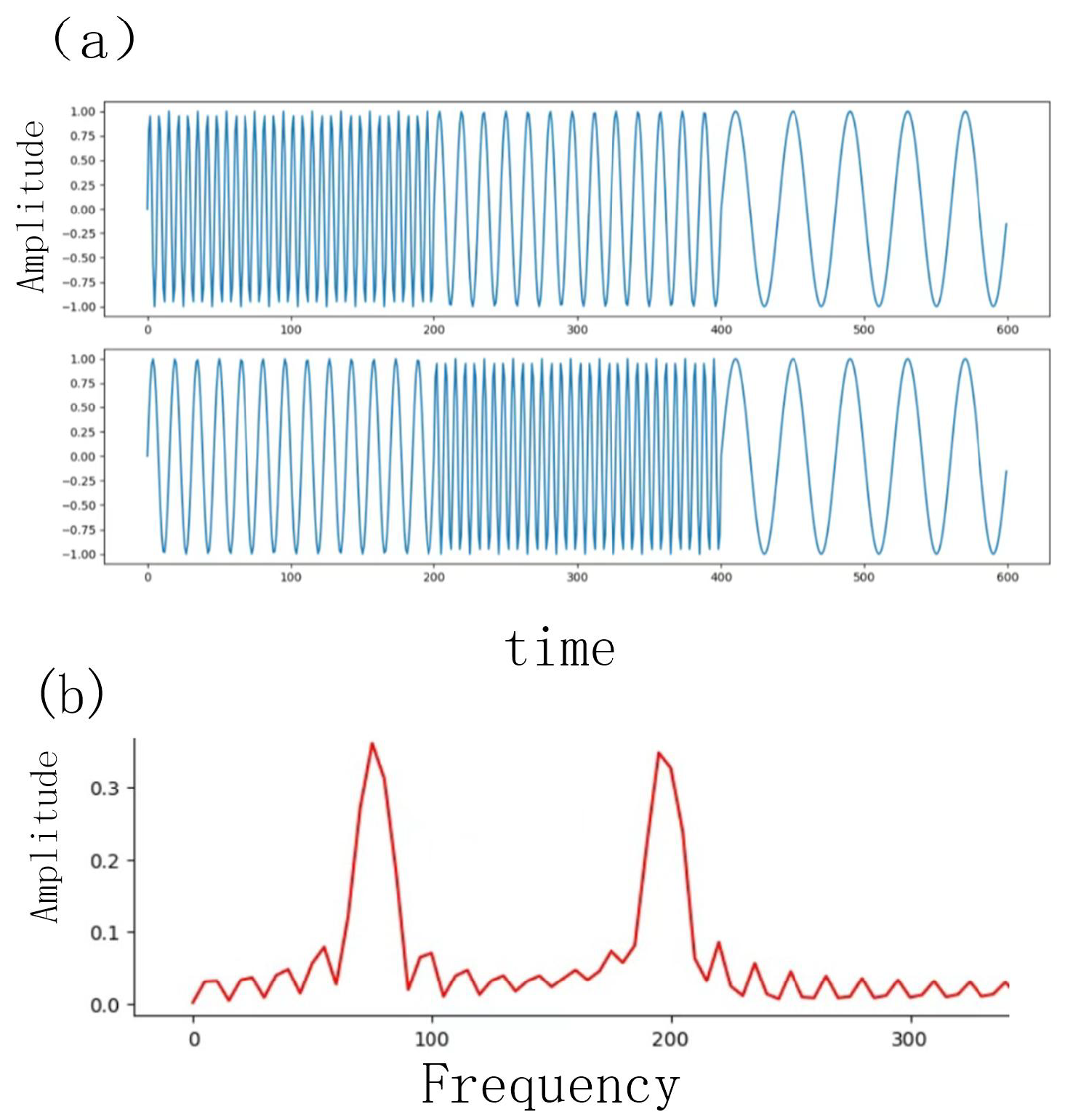
Figure 2.
The Transformer model architecture.
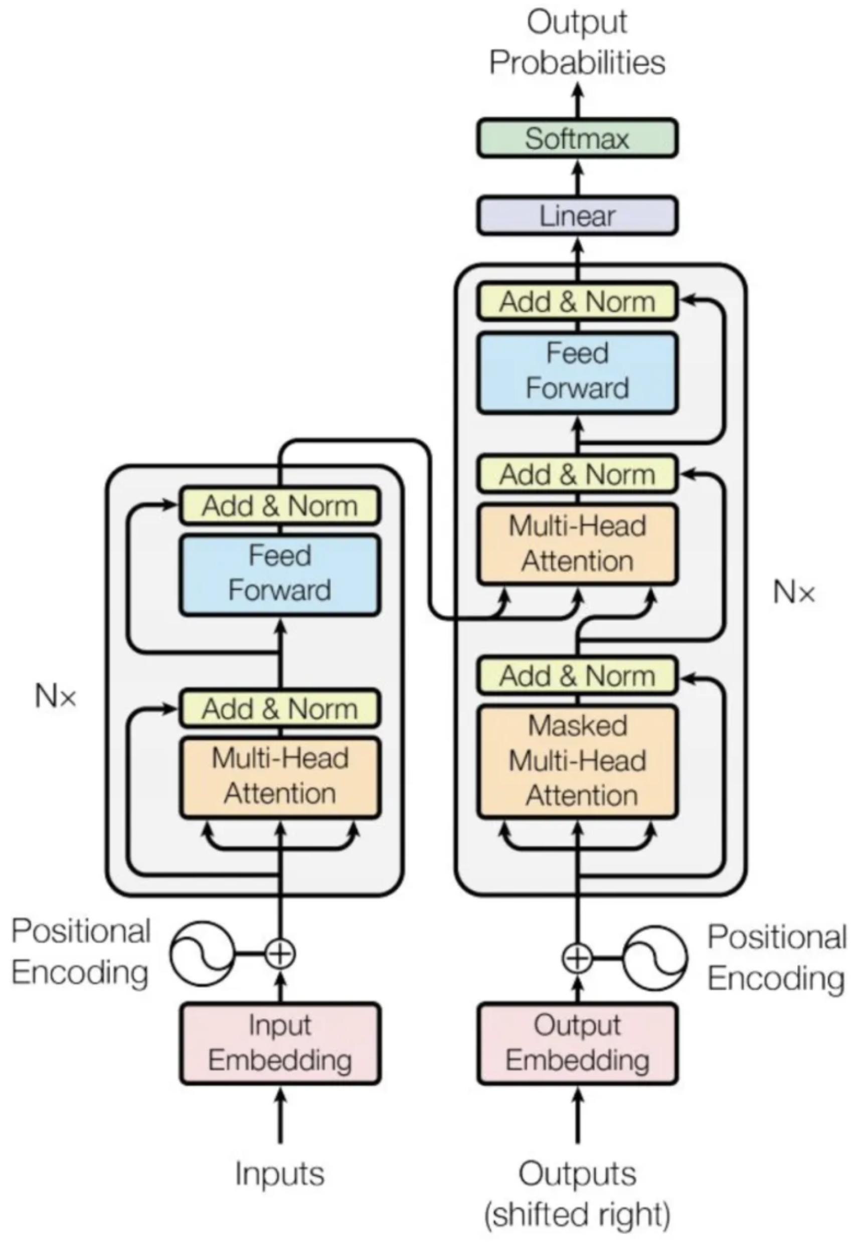
Figure 3.
Illustration of the (a) Block and (b) Wave-Net structures. Block serves as the basic building block of the Wave-Net model.
Figure 3.
Illustration of the (a) Block and (b) Wave-Net structures. Block serves as the basic building block of the Wave-Net model.
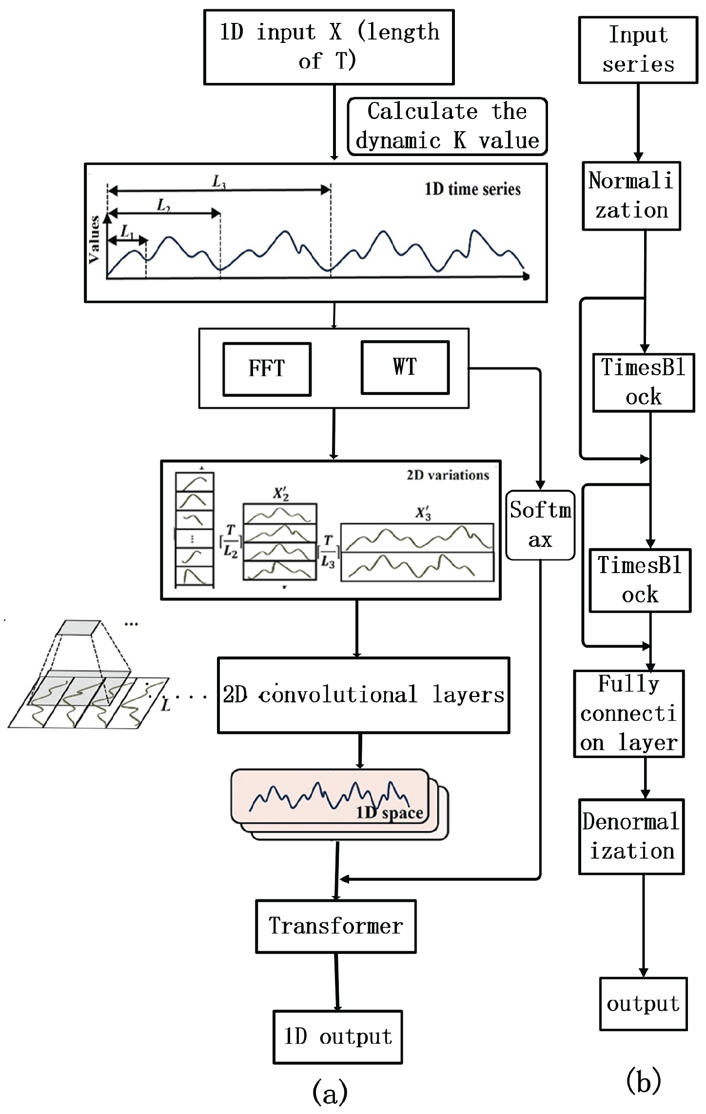

Table 1.
Potential Benefits of Learnable K.
| Dimension | Fixed K | Learnable K mechanism |
|---|---|---|
| Flexibility | No adaptive capacity | Dynamically adapted data characteristics |
| Multi-cycle capture | Possible omission of secondary cycle | Weighted use of all candidate cycles |
| Typical implementation | Hardcoded Top-K Selection | Dynamic screening of attention weights |
| Efficiency | High | Slightly below |
Table 2.
A summary of the benchmarks.
| Task | Benchmark | Metrics | Samples | Series-length | Dimension |
|---|---|---|---|---|---|
| Long-term forecasting | ETTH1 | MSE,MAE | 2785 | 96 | 7 |
| Long-term forecasting | Weather | MSE,MAE | 52696 | 96 | 14 |
| Long-term forecasting | Traffic | MSE,MAE | 17544 | 96 | 862 |
Table 3.
A detailed explanation of the fields in the ETTH1 dataset, including their corresponding Symbols, Explanation.
Table 3.
A detailed explanation of the fields in the ETTH1 dataset, including their corresponding Symbols, Explanation.
| Symbol | Explanation |
|---|---|
| Date | The recorded date |
| HUFL | High UseFul Load |
| HULL | High Useless Load |
| MUFL | Medium UseFul Load |
| MULL | Medium Useless Load |
| LUFL | Low UseFul Load |
| LULL | Low Useless Load |
| OT | Oil Temperature |
Table 4.
A detailed explanation of the fields in the Weather dataset, including their corresponding Symbols, Units and Explanation.
Table 4.
A detailed explanation of the fields in the Weather dataset, including their corresponding Symbols, Units and Explanation.
| Symbol | Unit | Explanation |
|---|---|---|
| Date Time | dd.mm.yyyy hh.mm (MEZ) | Date and time of the data record (the timestamp represents the end of the averaging period) |
| P | mbar | air pressure |
| T | °C | air temperature |
| Tpot | K | potential temperature |
| Tdew | °C | dew point temperature |
| rh | % | relative humidity |
| VPmax | mbar | saturation water vapor pressure |
| VPact | mbar | actual water vapor pressure |
| VPdef | mbar | water vapor pressure deficit |
| sh | gkg-1 | specific humidity |
| H2OC | mmolmol-1 | water vapor concentration |
| rho | gm-3 | air density |
| wv | ms-1 | wind velocity |
| max.wv | ms-1 | maximum wind velocity |
| wd | ° | wind direction |
| rain | mm | precipitation |
| raining | s | duration of precipitation |
| SWDR | Wm-2 | short wave downward radiation |
| PAR | mmolm-2s-1 | photosynthetically active radiation |
| max.PAR | molm-2s-1 | maximum photosynthetically active radiation |
| Tlog | °C | internal logger temperature |
| OT | ppm | CO2-concentration of ambient air |
Table 5.
A detailed explanation of the fields in the Traffic dataset, including their corresponding Symbols, Explanation.
Table 5.
A detailed explanation of the fields in the Traffic dataset, including their corresponding Symbols, Explanation.
| Symbol | Explanation |
|---|---|
| Date | Timestamp |
| 0-862 | Sensor node |
| OT | Proportion of vehicles occupying |
Table 6.
Comparison of the performance of multiple time series forecasting models on ETTH1, Weather, and Traffic tasks, using MSE and MAE as evaluation metrics.
Table 6.
Comparison of the performance of multiple time series forecasting models on ETTH1, Weather, and Traffic tasks, using MSE and MAE as evaluation metrics.
| ETTH1 | Weather | Traffic | ||||
|---|---|---|---|---|---|---|
| Model (Year) | MSE | MAE | MSE | MAE | MSE | MAE |
| ETSformer (2022) | 0.494 | 0.479 | 0.197 | 0.281 | 0.607 | 0.392 |
| LightTS (2022) | 0.424 | 0.432 | 0.182 | 0.242 | 0.615 | 0.391 |
| DLinear (2022) | 0.386 | 0.400 | 0.196 | 0.255 | 0.650 | 0.396 |
| FEDformer (2022) | 0.376 | 0.419 | 0.217 | 0.296 | 0.587 | 0.366 |
| Stationary (2022) | 0.513 | 0.491 | 0.173 | 0.223 | 0.612 | 0.388 |
| Autoformer (2022) | 0.449 | 0.459 | 0.226 | 0.336 | 0.613 | 0.388 |
| Pyraformer (2011) | 0.664 | 0.612 | 0.662 | 0.556 | 0.867 | 0.468 |
| Informer (2021) | 0.865 | 0.713 | 0.300 | 0.384 | 0.719 | 0.391 |
| LogTrans (2019) | 0.878 | 0.740 | 0.458 | 0.490 | 0.684 | 0.384 |
| Reformer (2020) | 0.837 | 0.728 | 0.689 | 0.596 | 0.732 | 0.423 |
| Wave-Net (Ours) | 0.398 | 0.418 | 0.176 | 0.226 | 0.588 | 0.315 |
Table 7.
Ablation of channel mix-up and channel attention with average MSE and MAE across prediction lengths.
Table 7.
Ablation of channel mix-up and channel attention with average MSE and MAE across prediction lengths.
| Wavelet transform | Fourier transform | Transformer | Wave-Net (MSE) | Wave-Net (MAE) |
|---|---|---|---|---|
| ✓ | – | ✓ | 0.4182 | 0.4321 |
| ✓ | – | – | 0.4256 | 0.4379 |
| ✓ | ✓ | – | 0.4129 | 0.4274 |
| ✓ | ✓ | ✓ | 0.3980 | 0.4186 |
Disclaimer/Publisher’s Note: The statements, opinions and data contained in all publications are solely those of the individual author(s) and contributor(s) and not of MDPI and/or the editor(s). MDPI and/or the editor(s) disclaim responsibility for any injury to people or property resulting from any ideas, methods, instructions or products referred to in the content. |
© 2025 by the authors. Licensee MDPI, Basel, Switzerland. This article is an open access article distributed under the terms and conditions of the Creative Commons Attribution (CC BY) license (http://creativecommons.org/licenses/by/4.0/).
Copyright: This open access article is published under a Creative Commons CC BY 4.0 license, which permit the free download, distribution, and reuse, provided that the author and preprint are cited in any reuse.


