
Submitted:
26 December 2025
Posted:
29 December 2025
You are already at the latest version
Abstract
Artificial neural networks (ANNs) are powerful models inspired by the structure and function of the human brain. They are widely used for tasks such as classification, prediction, and model recognition. This study examines the stability of fractional-order neural networks with neuronal conditions, dynamic behavior, synchronization, and delays of time. Synchronization and stability for delayed neural network models are two important aspects of dynamic behavior. For a calculated fractionalorder, the state of the state variable wi(t) are synchronized with each other. Weight synchronization of wi (i = 1, 2, 3, . . . ,6) provides coherent updates during training, helping neural networks to study stable models. The incommensurate fractional-orders are linked to a system where each dynamic component develops with a different value, i.e. qi ≠ qj (i ≠ j) is inconsistent. These fractionalorders are calculated for the system’s eigenvalues and their singular points within the stability region defined by the Matignon-based stability. As the time delay decreases, more activation functions are induced, and the variable state of w3(t) requires longer relaxation times to be more stable than the variable state of w4(t). The Grunwald-Letnikov method is used to solve a fractional neural network system numerically and effectively handle fractional derivatives. This approach helps to more accurately simulate memory in neural networks.
Keywords:
artificial neural networks
; stability analysis
; synchronization
; time delay
; dynamic systems
Introduction
Previous studies involved a variety of neurons with different delays. Many researchers are interested in analyzing neural networks. Many areas of science cover biological processes, automated control, brain modeling, sensor technology, computer vision, and more. [1,2,3]. Since 1984, Hopfield has presented many different classes of neural networks, but the dynamic properties of different types of neural connections have been shown to provide a wide range of applications in a variety of fields [4,5,6], including pattern recognition, control procedures, artificial intelligence, image processing, and medical science. In artificial neural networks, deadlines are often caused by inconsistencies in signal distribution between different neurons. To shed light on the reality of artificial neural networks [7], it is thought that neural network delays are made by a much better model compared to traditional neural networks without a temporary delay. Neural networks often exhibit much more, including periodic phenomena, unique chaotic properties, instability, and delays [8,9,10]. Currently, there is great interest in studying how different delays in the behavior of neural networks affect time delays. Currently, many neural network models are under construction and are being studied, with some interesting research published. Several researchers have studied the stability of wave outcomes in many models of neural networks based on distributed delayed cells. Various researchers [11,12] solve the problem of neural network synchronization.
As a result, there has been a growing interest in studying the latency of deep neural networks in recent years. Many important Indian artifacts have been created with brain structures that have been held in recent years. Global stabilization has been studied in quaternary artificial neural networks with temporary delays [13,14] using impulsive behavior and investigates modified saliva control to achieve complex delays in BAM structures. The research is a rather reliable criterion for ensuring the presence of global indices and periodic results of the quaternary nervous system with delays [15,16,17]. Stability analysis is performed due to the merits of regular outcomes of a particular type of discrepancy, the merits of the structures held by the BAM cognitive system compared to the D-operator, but the anti-periodic results of artificial neural networks, such as time and pulse, are also considered. The study randomly explores the stability of BAM network models jumping with delays [18,19,20].
Although the previously mentioned works have addressed some dynamic problems associated with delay, they concentrate on the integer-order component. In recent years, several academics have proposed that fractional-order differential equations are a better instrument for exposing the real-world linkages of dynamical systems since they are able to clarify over time ways of change and memory [21]. Recently, fractional calculus has been widely employed in different areas such as biology, electromagnetic waves, electrical technology, neuroscience, and financial management development [22,23,24]. Recently, fractional-order neural nets that handle delays have been the subject of appropriate research. Researchers [25] examined the global stability of fractional impulse delayed artificial neural networks and also investigated Mittag-Leffler transfer data in fractional-order octonion-valued [26] simulated neural network performance. The effect of leaking delay upon the Hopf bifurcation of fractional-order quaternion-valued computational neural networks [27]. Many researchers have found that voice, senses, robotics, understanding patterns, vision, and visual processing are very useful in the field of psychology [28,29].
In 1695, Leibniz and L’ Hospital traditionally explored the classical calculations that provided the main theory of fractional calculations. All natural explanations detected by fractional calculations are detected more accurately and accurately than regular calculations [30]. In 1832, the results were used to understand some mathematical problems. In 1892, Oliver published and developed a definition of division in a series of works. The main motivation for the invention of the entire Ford model was the lack of calculation results [31]. Using fractional-ordering, the ratio of voltage and currents for the most recent line of unstable half of the transmission is a great case [32,33]. Fractional derivatives can be easily modeled using a variety of numerical methods. Fractional calculus is used in research and research involving the fields of robotics, chemical interactions, biology, automation, technical theory, chaotic theory, and fractal structures. A system in which some variable fractional-orders are not proportional to one another is called incommensurate fractional-orders [34,35].
In previous studies, this indicates that most authors address the proportions with overall order issues and delays in neural networks. These models have been studied for fractional-orders of arbitrary values. This article provides a complex method for calculating inappropriate fractional-orders using clear points corresponding to unique values. Numerical analysis of neural network models occurs in the resulting stability domain based on these fractional-orders. Incommensurable fractional-orders help quickly and accurately converge your digital solutions. Using neural network models for incommensurable fractional-ordering, this study opens the way for new research fields over time. For fractional-order, calculated from neural network weights, the system remains synchronized and stable. The stable and convergent signals are shown in the graphical description of the synchronized scale of neural networks. This article investigates the stability of these networks with the evolution of temporary delays. In a fractional system, it is not an easy task to calculate the incommensurable fractional-orders.
Stability Analysis
Before discussing the reliability of the neural network model, it is impossible to calculate the incommensurate fractional-orders , where . For fixed values of the included parameters for the neural network model leads to a fractional-order system with the following form:
Select a random value from the parameters contained in the formats , and. Various singular points can be found in the model using the Jacobian matrix. Based on these balance points, the upper bounds of inappropriate fractional-order are calculated. and .
The stability region is defined by the Matignon-based stability [36].
where is the eigenvalue and is the incommensurate fractional-orders.
The corresponding fractional-order are calculated as and from the inequality (3.3). The incommensurate fractional-orders from to are physically stable because they lie in the first Riemann sheet region. On the other hand, does not lie in the stable region, which is not physical. It is possible to improve the reliability and stability of neural networks for a variety of practical purposes.
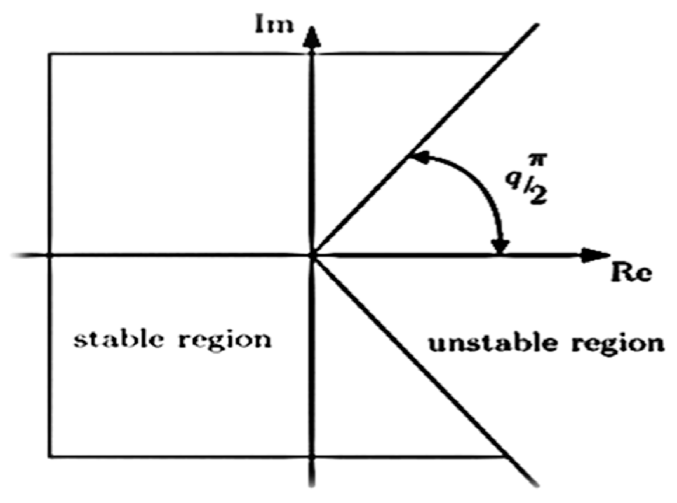
Figure 1.
Stability Region for Fractional-Order.
Mathematical Formulation
The neural network system is of the form [37]:
where and m represents the stability of internal neuron activities on the I-layer and J-layer, respectively. are time delays and indicate connecting weights through neurons. In two layers, the I-layer and the J-layer. The neurons on the I-layer whose states have been designated by receive the inputs and the inputs that those neurons in the J-layer output through activation functions , while the neurons on the J-layer whose associated states are revealed by obtain the inputs and the inputs that those neurons in the I-layer output via activation functions .
The schematic diagram (1.2) illustrates the main mechanisms of artificial neurons, the basic structural unit of neural networks. It starts with some input signals and, each associated with the corresponding weight and. An Artificial Neural Network consists of two key parts: one part is called the summation part, and the other is called the function part. Consider (for ) the neurons, then they are connected with their respective weight (for ), which is like connected with , connected with and so on. The summation part calculates the weighted sum in this form: and then forwards this weighted sum into the function part. The function part has a function called an activation function , which generates a particular output for a given input. The arrows in the diagram indicate the flow of input data through the total and activation stages at the final output . This process models how artificial neurons mimic human mind, integrate several signals, and make decisions.
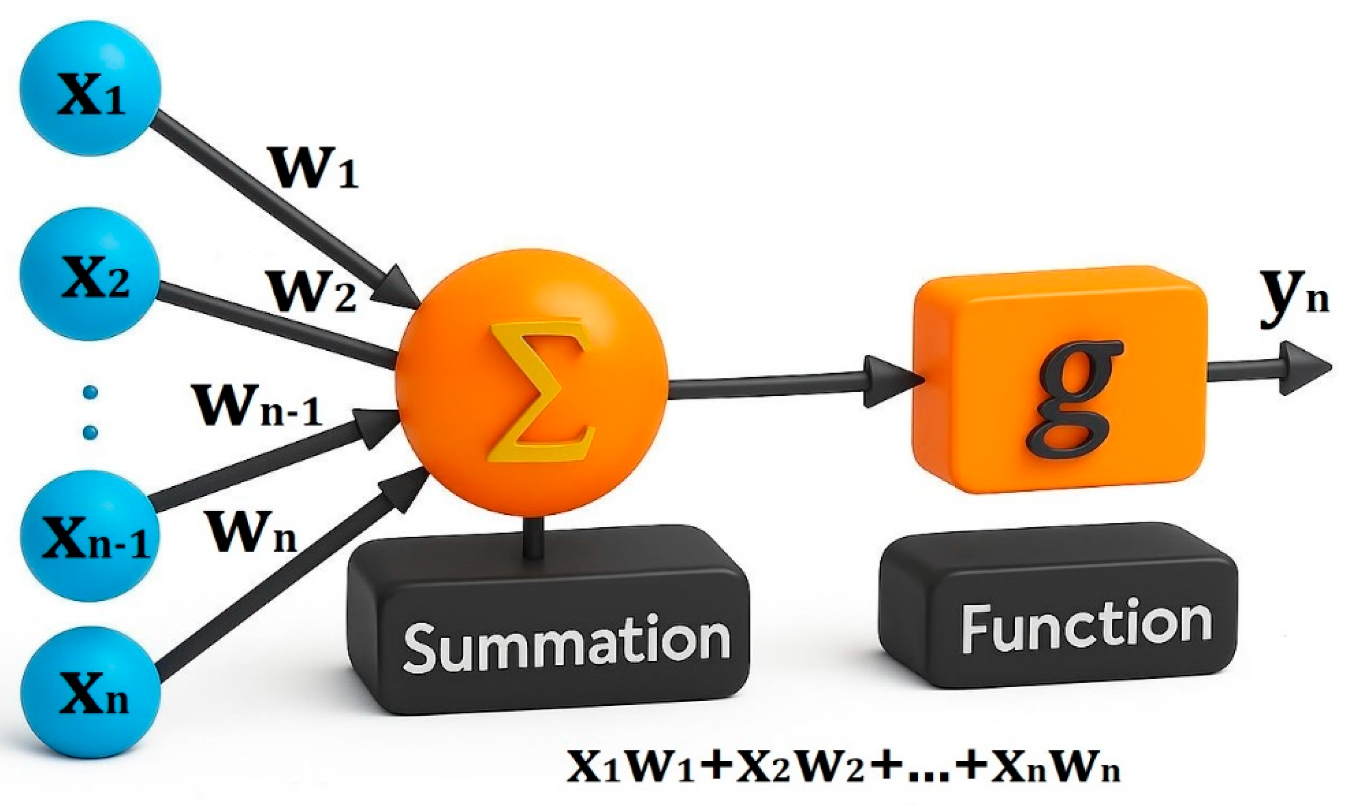
Figure 2.
Schematic Diagram.
The formulation of a model for an artificial neural network is the topic discussed in this part. The model concerning the delayed neural networks is given [38]:
where represents the training parameter, and are the activation functions.
In general, consider and and where b and are all real. The system (1.4) takes the form:
The system (1.5) can be modified for incommensurate fractional-orders as:
where are the incommensurate fractional-orders.
Numerical Solution
For numerical calculation of fractional-order derivatives, the required equation can be derived from the Grunwald-Letnikov fractional-order derivative. The relation to the explicit numerical approximation of derivative at the points , () has the following form [39]:
where is the “memory length”, , is the time step of calculation, and are binomial coefficients (). For their calculation, we can use the following expression [39]:
The general numerical solution of the fractional differential equation is
The numerical solution can be expressed as:
For the memory term expressed by the sum, a short memory principle can be used.
In addition, it uses a more convenient numerical solution of the fractional-order Eq. (1.1), which is based on the Grunwald-Letnikov method. It will take the following form:
where and is the start point. The binomial coefficients are calculated according to Eq. (1.8). All simulations were performed for time step
Graphical Results
Figure 3.
Time Evolution of Stable Oscillations with Complex Amplitude Modulation.
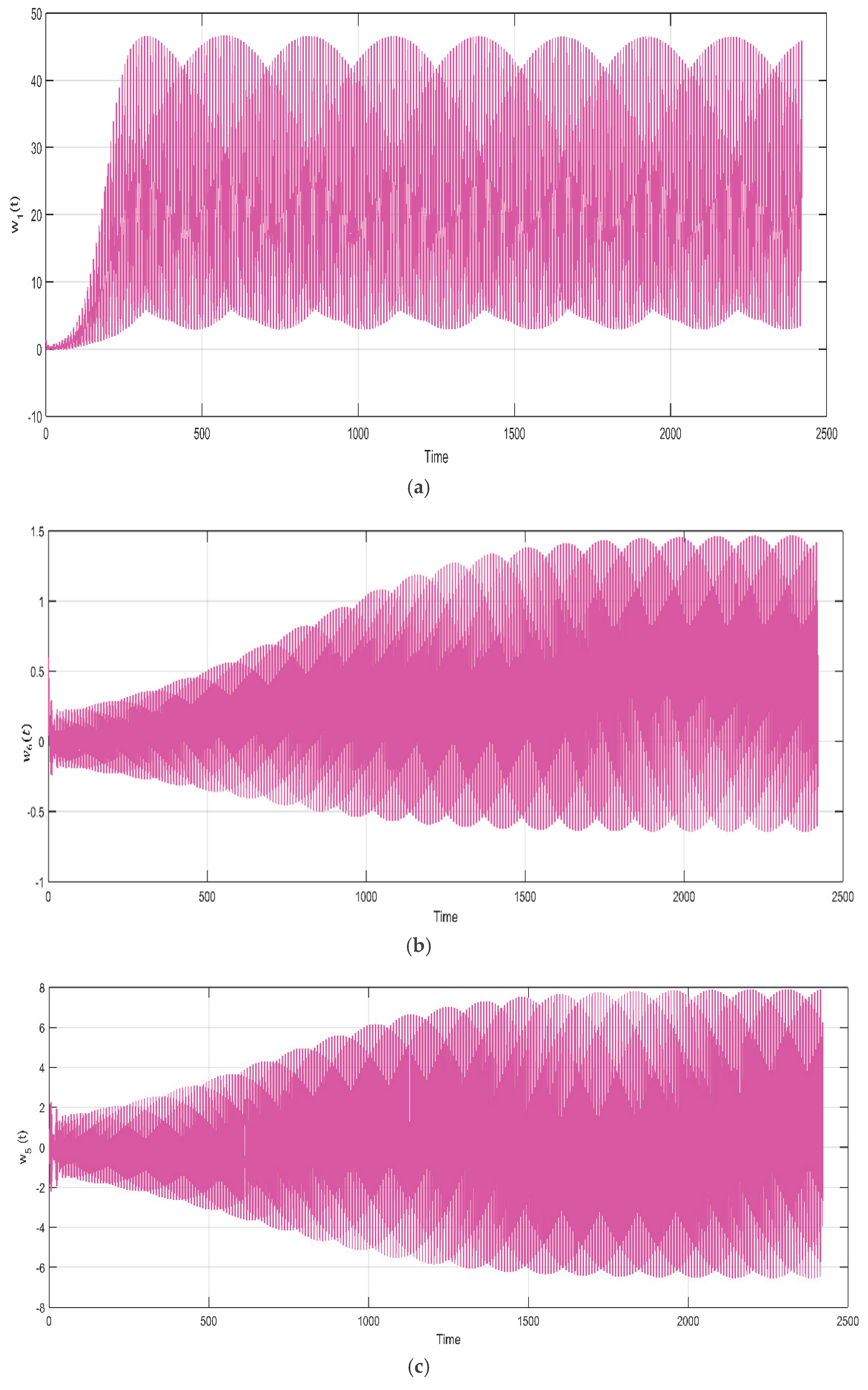
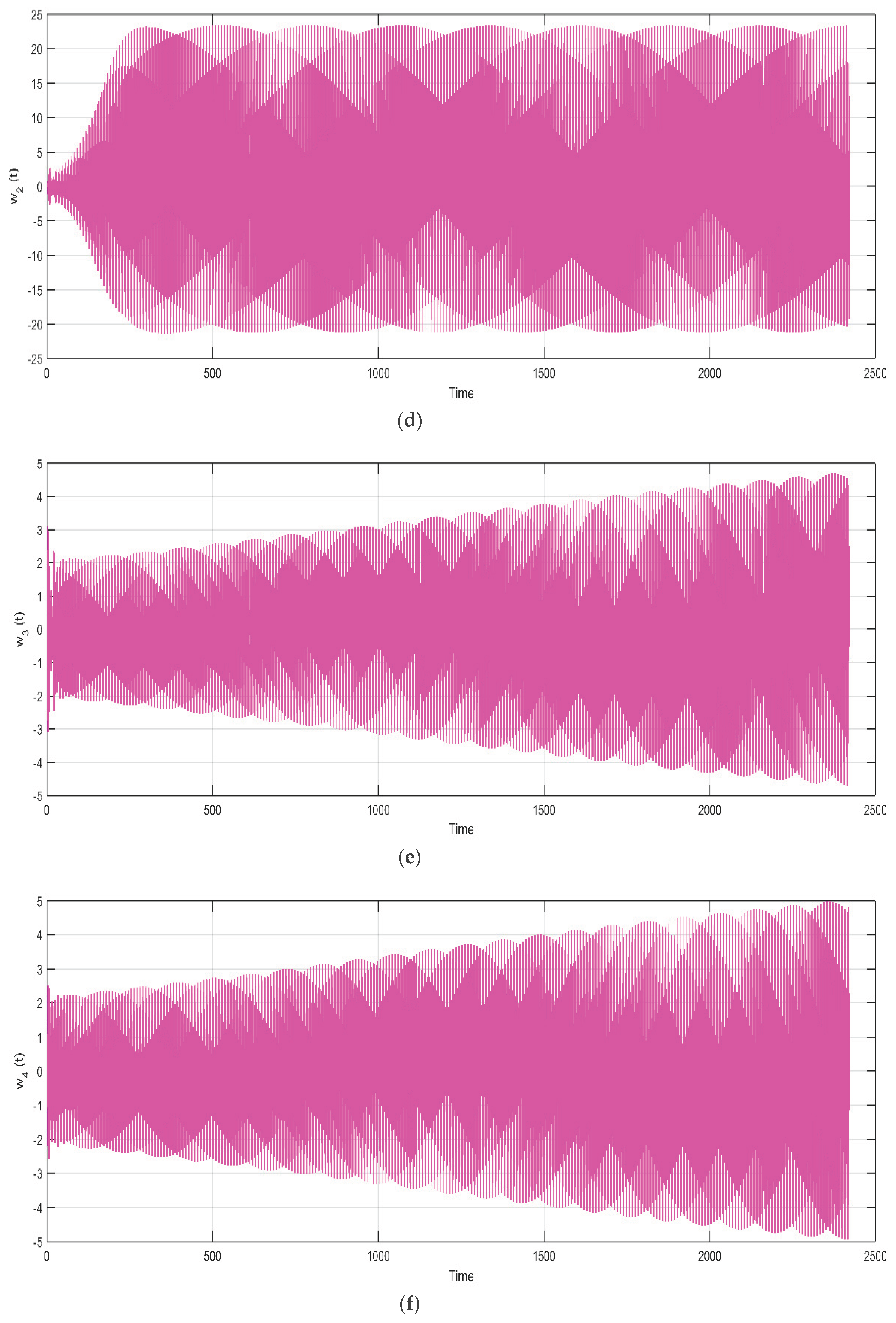
Figure 4.
Weighted Synchronization of State Variables , , , and .

Discussion
The evolution of the neuron state over time, approximately units, is depicted in time series results plot 1.3 (a). Initially, with , the state parameter fluctuates between and. By , the amplitude increases by about units, indicating heightened neuron activity. The variation stabilizes around units, peaking approximately units post-transition, influenced by a fractional-orders qi affecting the system's behavior. From time 0 to 2400, oscillates with amplitude increasing from toby. The signal contains frequencies between 0.02 Hz and 0.12 Hz, indicating propagation and resonance, which highlights the neural network's dynamic adaptability. Plot 1.3 (b) reveals a unique repeated modulation pattern and smooth pulsating behavior, suggesting steady interaction frequencies from a fractional-order neural network. The oscillations in graph 1.3 (c) of vary from to over to temporal units. At , periodic amplitude modulation occurs, with peaks rising from about to . Interference patterns reveal beat frequencies from multiple sinusoidal components at Hz and Hz. From to units in Figure 3 (d), the state variable exhibits oscillations with amplitudes between and. Fluctuations are erratic when , peaking at and around Hz. The variation is stabilized by about 3 units at t = 500, forming an almost auxiliary image with a frequency of about Hz, reflecting the transition of the synchronized state. Sketch 1.3 (e) represents the variable state that fluctuates between andin units. The amplitude modulation passes from about to about around , forming the shape of the shell. The frequency of vibrations varies from 0.02 Hz to 0.1 Hz, revealing the effects of typical memory and nonlinear feedback in fractional-order neural networks. The envelope period of about units indicate synchronization regime changes significant for modeling brain dynamics. The amplitude oscillations in 1.3 (f), range from to and peaking at nearly by . The shape of the waves shows modulation similar to the envelope with several frequency components that exhibit irregular interactions common in fractional-order neural networks. Significant oscillation frequency is between Hz and Hz, indicating the transition from an inactive oscillating neural state to a controlled one.
In plot 1.4(a), versus shows a limited elliptical trajectory that is central at the beginning of the coordinates, fluctuating between and, indicating stable behavior. This closed-loop pattern demonstrates synchronization between neuron states influenced by fractional-order dynamics. The system's smooth evolution in a limited phase space aligns with stability criteria. The phase graph 1.4 (b) of and illustrates a bounded elliptical pattern centered at the origin, with values ranging from to and w₁(t) from to, indicating stable, periodic oscillations influenced by fractional-order dynamic model. The sketch 1.4 (c) displays a dense elliptical shape for and , indicating confined states and system stability. Different dynamical scales lead to regular oscillations without chaotic behavior.
The phase Figure 5 (a) of versus displays a dense elliptical shape, indicating strong correlation and synchronization, with values between and. This pattern's fine oscillation suggests multiple frequency components interacting nonlinearly, characteristic of fractional-order neural networks influenced by memory effects with a fractional-order q around 0.9. In Figure 5 (b), against presents a confined elliptical pattern between and, indicating bounded trajectories, which denotes stability without divergence. The multiple interacting frequencies of the system operates in a stable, synchronized regime rather than exhibiting chaotic behavior.
Conclusions
The neuron states become unstable whenever the incommensurate fractional-orders exceeds their upper bounds. A congested stability within the interval and a chaotic effect beyond this interval of neuron state synchronized against are reported. The reduction of the time delay will give more relaxation time for the state variable to be stable as compared to the state variable . The exclusion of two neuron states and , enhances the stability of the system. The enhancement of stability in Figure 5 (b) is reasoned out by the addition of the extra parameter . The setup of the parameter at 12.2 enabled the trained the system consistent and allow the model to converge successfully without ambiguity.
Nomenclature
| Symbols | Representations |
| Fractional-order derivative. | |
| Incommensurate fractional-orders | |
| Real numbers | |
| Time | |
| Time delay | |
| State Variables or Neuron States | |
| Training Parameter | |
| Activation Functions | |
| Connecting Weights Through Neurons | |
| Stability of Internal Neuron Activities |
References
- Li, Y., & Shen, S. (2020). Almost automorphic solutions for Clifford-valued neutral-type fuzzy cellular neural networks with leakage delays on time scales. Neurocomputing, 417, 23-35. [CrossRef]
- Xiu, C., Zhou, R., & Liu, Y. (2020). New chaotic memristive cellular neural network and its application in a secure communication system. Chaos, Solitons & Fractals, 141, 110316. [CrossRef]
- Ji, L., Chang, M., Shen, Y., & Zhang, Q. (2020). Recurrent convolutions of binary-constrained cellular neural network for texture recognition. Neurocomputing, 387, 161- 171. [CrossRef]
- Kumar, R., & Das, S. (2020). Exponential stability of inertial BAM neural network with time-varying impulses and mixed time-varying delays via matrix measure approach. Communications in Nonlinear Science and Numerical Simulation, 81, 105016. [CrossRef]
- Xu, C., Liao, M., Li, P., Liu, Z., & Yuan, S. (2021). New results on pseudo almost periodic solutions of quaternion-valued fuzzy cellular neural networks with delays. Fuzzy Sets and Systems, 411, 25-47. [CrossRef]
- Kobayashi, M. (2021). Complex-valued Hopfield neural networks with real weights in synchronous mode. Neurocomputing, 423, 535-540. [CrossRef]
- Cui, W., Wang, Z., & Jin, W. (2021). Fixed-time synchronization of Markovian jump fuzzy cellular neural networks with stochastic disturbance and time-varying delays. Fuzzy Sets and Systems, 411, 68-84. [CrossRef]
- Huang, C., Su, R., Cao, J., & Xiao, S. (2020). Asymptotically stable high-order neutral cellular neural networks with proportional delays and D-operators. Mathematics and Computers in Simulation, 171, 127-135.
- Meng, B., Wang, X., Zhang, Z., & Wang, Z. (2020). Necessary and sufficient conditions for normalization and sliding mode control of singular fractional-order systems with uncertainties. Science China Information Sciences, 63, 1-10. 20. [CrossRef]
- Hsu, C. H., & Lin, J. J. (2019). Stability of traveling wave solutions for nonlinear cellular neural networks with distributed delays. Journal of Mathematical Analysis and Applications, 470(1), 388-400. [CrossRef]
- Li, Y., & Qin, J. (2018). Existence and global exponential stability of periodic solutions for quaternion-valued cellular neural networks with time-varying delays. Neurocomputing, 292, 91-103. [CrossRef]
- Tang, R., Yang, X., & Wan, X. (2019). Finite-time cluster synchronization for a class of fuzzy cellular neural networks via non-chattering quantized controllers. Neural Networks, 113, 79-90. [CrossRef]
- Wang, W. (2018). Finite-time synchronization for a class of fuzzy cellular neural networks with time-varying coefficients and proportional delays. Fuzzy Sets and Systems, 338, 40-49. [CrossRef]
- Wang, S., Zhang, Z., Lin, C., & Chen, J. (2021). Fixed-time synchronization for complex-valued BAM neural networks with time-varying delays via pinning control and adaptive pinning control. Chaos, Solitons & Fractals, 153, 111583. [CrossRef]
- Zhao, R., Wang, B., & Jian, J. (2022). Global stabilization of quaternion-valued inertial BAM neural networks with time-varying delays via time-delayed impulsive control. Mathematics and Computers in Simulation, 202, 223-245.
- Kong, F., Zhu, Q., Wang, K., & Nieto, J. J. (2019). Stability analysis of almost periodic solutions of discontinuous BAM neural networks with hybrid time-varying delays and D-operator. Journal of the Franklin Institute, 356(18), 11605-11637. [CrossRef]
- Xu, C., & Zhang, Q. (2014). On the antiperiodic solutions for Cohen-Grossberg shunting inhibitory neural networks with time-varying delays and impulses. Neural Computation, 26(10), 2328-2349. [CrossRef]
- Ali, M. S., Yogambigai, J., Saravanan, S., & Elakkia, S. (2019). Stochastic stability of neutral-type Markovian-jumping BAM neural networks with time-varying delays. Journal of Computational and Applied Mathematics, 349, 142-156. [CrossRef]
- Cong, E. Y., Han, X., & Zhang, X. (2020). Global exponential stability analysis of discrete-time BAM neural networks with delays: A mathematical induction approach. Neurocomputing, 379, 227-235. [CrossRef]
- Ayachi, M. (2022). Measure-pseudo almost periodic dynamical behaviors for BAM neural networks with D operator and hybrid time-varying delays. Neurocomputing, 486, 160-173. [CrossRef]
- Shi, J., He, K., & Fang, H. (2022). Chaos, Hopf bifurcation, and control of a fractional-order delay financial system. Mathematics and Computers in Simulation, 194, 348-364. [CrossRef]
- Xiao, J., Wen, S., Yang, X., & Zhong, S. (2020). New approach to global Mittag-Leffler synchronization problem of fractional-order quaternion-valued BAM neural networks based on a new inequality. Neural Networks, 122, 320-337. [CrossRef]
- Xu, C., Mu, D., Pan, Y., Aouiti, C., Pang, Y., & Yao, L. (2022). Probing into bifurcation for fractional-order BAM neural networks concerning multiple time delays. Journal of Computational Science, 62, 101701. [CrossRef]
- Xu, C., Liao, M., Li, P., Guo, Y., & Liu, Z. (2021). Bifurcation properties for fractional-order delayed BAM neural networks. Cognitive Computation, 13, 322-356. [CrossRef]
- Wang, F., Yang, Y., Xu, X., & Li, L. (2017). Global asymptotic stability of impulsive fractional-order BAM neural networks with time delay. Neural Computing and Applications, 28, 345-352. [CrossRef]
- Ye, R., Liu, X., Zhang, H., & Cao, J. (2019). Global Mittag-Leffler synchronization for fractional-order BAM neural networks with impulses and multiple variable delays via delayed-feedback control strategy. Neural Processing Letters, 49, 1-18. [CrossRef]
- Xu, C., Liu, Z., Aouiti, C., Li, P., Yao, L., & Yan (2022). New exploration on bifurcation for fractional-order quaternion-valued neural networks involving leakage 22 delays. Cognitive Neurodynamics, 16(5), 1233-1248.
- Xiao, J., Guo, X., Li, Y., Wen, S., Shi, K., & Tang, Y (2022). Extended analysis on the global Mittag-Leffler synchronization problem for fractional-order octonion-valued BAM neural networks. Neural Networks, 154, 491-507. [CrossRef]
- Popa, C. A. (2023). Mittag-Laffler stability and synchronization of neutral-type fractional-order neural networks with leakage delay and mixed delays. Journal of the Franklin Institute, 360(1), 327-355. [CrossRef]
- Ci, J., Guo, Z., Long, H., Wen, S., & Huang, T. (2023). Multiple asymptotic periodicities of fractional-order delayed neural networks under state-dependent switching. Neural Networks, 157, 11-25.
- Shah, D. K., Vyawahare, V. A., & Sadanand, S. (2025). Artificial neural network approximation of special functions: design, analysis, and implementation. International Journal of Dynamics and Control, 13(1), 1-23. [CrossRef]
- Admon, M. R., Senu, N., Ahmadian, A., Majid, Z. A., & Salahshour, S. (2024). A new and modern scheme for solving fractal-fractional differential equations based on a deep feedforward neural network with multiple hidden layers. Mathematics and Computers in Simulation, 218, 311-333. [CrossRef]
- Maurya, S. S., Kannan, J. B., Patel, K., Dutta, P., Biswas, K., Santhanam, M. S., & U. D. (2024). Asymmetric dynamical localization and precision measurement of the micromotion of a Bose-Einstein condensate. Physical Review A, 110(5), 053307. [CrossRef]
- Joshi, D. D., Bhalekar, S., & Gade, P. M. (2024). Stability analysis of fractional differential equations with delay. Chaos: An Interdisciplinary Journal of Nonlinear Science, 34(5).
- Chettouh, B. (2024). Stability, Bifurcations and Control in Fractional-order Chaotic Systems (Doctoral dissertation, Université Mohamed Khider (Biskra-Algérie)).
- Ur Rahman, H., Shuaib, M., Ismail, E. A., & Li, S. (2023). Enhancing medical ultrasound imaging through fractional mathematical modeling of ultrasound bubble dynamics. Ultrasonics Sonochemistry, 100(9), 106603. [CrossRef]
- Gopalsamy, K., & He, X. Z. (1994). Delay-dependent stability in bidirectional associative memory networks. IEEE Transactions on Neural Networks, 5(6), 998-1002.
- Zhang, C., Zheng, B., & Wang, L. (2009). Multiple Hopf bifurcations of a symmetric BAM neural network model with delay. Applied Mathematics Letters, 22(4), 616-622. [CrossRef]
- Vinagre, B. M., Chen, Y. Q., & Petráš, I. (2003). Two direct Tustin discretization methods for a fractional-order differentiator/integrator. Journal of the Franklin Institute, 340(5), 349-362.
Figure 5.
Weighted Synchronization of State Variables , and .

Disclaimer/Publisher’s Note: The statements, opinions and data contained in all publications are solely those of the individual author(s) and contributor(s) and not of MDPI and/or the editor(s). MDPI and/or the editor(s) disclaim responsibility for any injury to people or property resulting from any ideas, methods, instructions or products referred to in the content. |
© 2025 by the authors. Licensee MDPI, Basel, Switzerland. This article is an open access article distributed under the terms and conditions of the Creative Commons Attribution (CC BY) license (http://creativecommons.org/licenses/by/4.0/).
Copyright: This open access article is published under a Creative Commons CC BY 4.0 license, which permit the free download, distribution, and reuse, provided that the author and preprint are cited in any reuse.


