
Submitted:
04 October 2025
Posted:
06 October 2025
You are already at the latest version
Abstract
An automated learning process is a powerful tool that extracts useful data structures by measuring information, expressing conditions, and regulating invariant tolerance. Surveillance video systems and intelligent video analysis have become increasingly valuable, as it is often challenging to discern and represent the primary motion patterns necessary for automatic analysis. Combining automated learning with video analysis enables the development of intelligent analytic systems that can operate effectively in uncertain scenarios, automatically identifying dominant motion dynamics. The ability to recognize these motion dynamics relies on the theoretical framework used to represent them and the learning process employed to identify patterns. In the literature, a state-system-based approach offers a way to describe temporal and spatial interrelationships, which is essential for understanding motion dynamics. A key aspect of this approach is determining when the number of positive learned states from a given information source becomes sufficient to detect dominant motion in a surveillance video system. This determination is crucial as it impacts the variability of movements that the monitored subjects can exhibit while adhering to the camera’s view projection and the resources required for implementation. While previous research has produced practical approaches, most have been limited to specific scenarios, underscoring the need for further investigation. In this study, we outline several advantages of establishing a formal criterion to determine when a symbolic system in a surveillance scenario has developed a robust and practical model to explain the observed motion dynamics. Our proposal is sustained by the hypothesis that a correct model can reliably account for most motion dynamics over time in an automatic learning process. The validation is performed with different real scenarios, where the central dynamic becomes learned, labeling those dynamics that the learned model cannot explain. In a real application, the approach was used to model traffic vehicles on the avenues of Queretaro City.
Keywords:
smart surveillance
; automatic learning
; motion dynamic patterns
; modelling
1. Introduction
In rapidly growing cities, it is common to implement and integrate low-cost video surveillance systems that can operate effectively in various environmental conditions, both indoors and outdoors. This generates a massive volume of information, which is impossible to analyze comprehensively. From this perspective, it is necessary to integrate intelligent systems that assist in processing this information, with an emphasis on detecting and analyzing events of interest [1,2]. The detection of these events is particularly relevant in applications aimed at crime prevention, tracking persons of interest [3], detecting atypical behavior [4,5], optimizing resources [6], and crowd dynamics analysis [7].
The literature review identifies the main variables that affect the effectiveness of existing techniques, classifying them as follows: i) the quality of the data collected, since its accuracy and completeness directly impact the effectiveness of the process [8,9,10]; ii) the frequency of sampling data, referring to the periodicity with which the data is renewed, which significantly influences the ability to detect activities of interest [11]; iii) coverage or scope, which determines the susceptibility of events to be detected as a result of the perspective of the cameras and possible occlusions present in the scene associated with the semantic of the dynamic observed [12,13,14]; and finally, iv) the sensitivity of the system, referring to the detection threshold that allows us to distinguish between an event of interest and a possible false positive [15,16,17].
In this context, intelligent surveillance systems employ adaptive machine learning techniques that enable the identification and extraction of movement patterns, thereby representing the dynamics of the scene. For this purpose, the algorithms prioritize two aspects: the way in which movement is defined in the scene and the way in which the structures of that movement are modeled.
In the first step, the criteria for encoding information are analyzed so that, once the data of interest has been expressed, it can be processed in a compact manner consistent with the semantics of the objects’ dynamics present in the scene. Under this criterion, some studies use segmentation masks that delimit the regions occupied by the object in the scene [18]. Other approaches consider the region of interest through silhouettes as binary masks or heat maps, where the objects of interest correspond to the pixels with the highest value. In contrast, irrelevant information approaches values close to zero[19,20,21]. In addition, there are innovative approaches based on deep neural networks that extract relevant attributes such as the position, aspect ratio, and height of objects [22,23]. The second criterion analyzes the structures that allow movement structures to be grouped and modeled, which in turn can be: (i) by perimeter delimitation of the geometry of the shape, which considers information about the texture or color of objects to identify them and enclose them in a space that can be rectangular, square, or elliptical [24], some based on object contours [25,26], these works implement length and area restrictions on the region to be segmented by means of cost functions, in particular [27] applies methods based on convolutional neural networks (CNN); (ii) using hierarchical structures based on enumeration, some representative works are [28,29], where they use multiscale inference approaches under the approach of combining multiscale predictions.
For cases where it is necessary to model the dynamics of the scene, allowing the detection of the dominant dynamics for the description of activities over time, this is of interest in automatic monitoring activities, where the objective is usually to recognize and differentiate the observed activities [30,31,32]. To this end, different techniques have been developed that consider information about movement in the scene as evidence to infer models capable of describing the observed activities.
The efficiency of these models depends entirely on the learning processes implemented, as the proper definition of movement rules in a scenario directly impacts the efficiency of monitoring and security systems [2]. For this reason, the ability to identify relevant movement patterns in a scenario is a fundamental task for detecting or omitting events that may be considered of interest in monitoring applications.
Currently, there are tasks for which no general solution exists [33,34]. Efforts are focused on solving challenges such as missing information resulting from random or deterministic factors, which motivates strategies based on techniques like k-nearest neighbors (KNN) and missForest [35], among others. Another challenge arises when algorithms and criteria require a minimum amount of information for learning, as well as full knowledge of the number of rules needed to represent the data. Along the same lines, Callaghan et al. [36] highlight the importance of establishing reliable criteria for evaluating the sufficiency of the information learned and used in different algorithms, identifying this need as a current research gap.
These approaches fall into four main categories: (i) sampling-based criteria, where the expert estimates the amount of relevant information through random sampling at the beginning of the process, stopping the process when the target set by the expert system is reached; (ii) heuristic-based techniques, where detection occurs when a certain amount of information irrelevant to the process is detected; (iii) pragmatic criteria, which set a predefined learning time for the system, adjusted to the application case, achieving low efficiency; and (iv) new automatic detection criteria, which implement novel and complex approaches to automatically decide when to stop the learning process, based on specific metrics.
This work introduces a sufficiency criterion for determining the optimal number of rules learned by a system based on motion states, to model the overall dynamics of the system.
This criterion is based on the concept of maximum entropy applied to new rules generated over time, which is particularly useful in systems with locally stationary dynamics. The system segments the camera’s field of view into areas with a high-state probability of movement, then classifies these states into disjoint and connected sets, each of which is assigned a symbolic label. Over time, the system generates sequences of motion symbols, which are ultimately organized into a grammatical structure that models the succession of states using an automated criterion [37,38]. The grammatical structure becomes inferred by taking the emitted words as positive samples of the common dynamics sampled. Then, the system represents the dynamics of movement in video scenarios, using grammatical inference to identify recurring patterns and a formal criterion of sufficiency that determines when the system has achieved learning stability.
Referring to the above paragraphs, the most relevant contributions of this research are:
- The definition of a formal criterion of information sufficiency that determines when the system has reached grammatical stability.
- The criteria exploit the properties of periodic systems, based on information criteria to learn the most significant grammar rules.
- A discrete model criteria based on right grammars to symbolically represent movement trajectories in video sequences.
- A criterion to encode a state-based system, the different trajectories through the SEQUITUR approach for inferencing the grammar structure in the most compact representation of movement patterns.
2. Proposed Model
This proposal describes a state-based model, where each state represents a spatial area of the camera’s field of view projection. A set of adjacent and connected pixels defines each state. The states do not overlap, so that the activation of a state (indication of movement) is considered a probability function of the variability of the intensity of the pixels that compose it. States with a high probability of variability are considered active and are subject to change over time. Thus, the dynamics of an object moving through the scene are expressed as a sequence of state activations over time.
The structures of observable dynamics are characterized by a stack automaton, which enables the modeling of object movements hierarchically in the form of a proper grammar. The grammar representing the movement is constructed using the Sequitur algorithm, which infers a hierarchical structure from a sequence of discrete symbols [37]. This approach enables the modeling of dynamics using hierarchical structures, and the process of verifying whether the dynamics are associated with the model involves determining, through the grammar, whether the previously defined structures can explain the sequence of activated states.
The formal description of the proposal is expressed as follows: Let the workspace V be a grid space representing the two-dimensional projection of the camera’s field of view with dimensions . Each position in the workspace represents the intensity of the pixel at position on the image. Then, the possible number of states (partitions) of the workspace V is determined by . In this case, a state is a valid state if and only if, for the state and for every tuple where , there is at least one connected path between both points. Then, the set of states of the system is determined by , where each state is disjoint from the others, but may or may not be adjacent to others.
On the other hand, if there is evidence that any object occludes a state, it can be calculated using temporal contrast dynamics. That is, when there is a significant change in the intensities of the pixels that comprise it, the state is considered to be occluded and, consequently, to exhibit movement. The motion equation is defined in Equation (1).
The values of and the estimate of P represent the confidence/certainty of motion detection and the process for estimating probability. The function allows us to determine whether the state e has motion or not at time t. To symbolically represent the active states, an alphabet is defined. From this, a bijective subset is constructed, which uniquely associates each active state e with a symbol from the alphabet , thus allowing the generation of symbolic sequences associated with the dynamics of the system.
Finally, the function allows us to know, in terms of the alphabet , the states that have a probability of movement , which is defined in .
The function assigns a unique symbol to each state that has a significant probability of movement. This assignment is made under the condition imposed by the detection criterion , which evaluates whether the state e has a probability of movement greater than a defined threshold . Consequently, the function assigns symbols from the alphabet only to those states that have been classified as active. In this way, the movement over the scene activates a set of states, which under produce a sequence of strings emitted by the scenario. These sequences become used to build the grammar of the dynamic movement. In a current frame, more than one state becomes activated for the movement appreciated in the scene. In these cases, the strings become concatenated with only adjacent states, which avoids the use of non-connected movements, and reduces to the use of only strings generated with temporal adjacent motion evidence to infer the grammar.
Finally, discrete sequences are used to infer grammars , considering each emitted string as a positive sample of the grammar. These grammars enable the identification of recurring movement patterns, which are expressed through grammatical rules . By applying the properties of SEQUITUR in the generation of rules, it is possible to construct hierarchical representations of the observed behavior.
With this approach, it is possible to establish a criterion for learning sufficiency , based on grammatical stability. This criterion is formalized as , where represents the number of rules inferred for the representation of in the i-th sequence. This criterion indicates that when a point is reached at which the number of rules generated between sequences and satisfies , the system has stabilized its knowledge and captured the main dynamics of the environment.
2.1. Motion Modeling
Within the study of computer vision-based learning methods, various techniques have been proposed for representing motion information, as discussed in [31,39], which offer interesting proposals for extracting motion patterns. One of these approaches can be represented by the following expression.
where represents the motion information of the objects in the scene, and denotes the intensity of the pixel at position at time instant t. The difference between the intensity values at two consecutive time instants t and allows us to estimate the change associated with the motion. From this information, it is possible to obtain the trajectories of the moving objects, represented as the set . The information on the movement pattern generated by an object, throughout a sequence of images at a given time t, is expressed as , where each element corresponds to a spatial position occupied by the i-th object at a time t [40].
2.2. Trajectory Generation Process
In the process of generating trajectories, various techniques help increase the expressiveness of the representation of motion information, among which the binarization of trajectories [41,42], N-tuples, symbol strings [43], among others, stand out. Each has its advantages and limitations, depending on the specific case study. To provide a clearer view of the alternatives reported in the literature, Table 1 summarizes representative motion coding techniques applied in similar contexts. This comparison highlights the diversity of state definitions and coding strategies, offering a reference framework for positioning the present work within the field.
Following this analysis, our approach adopts a representation based on symbol strings [44], which offers an effective solution to the problem of trajectory expressiveness . The new representation of trajectories begins with the definition of regions belonging to the movement E and is formalized by the function , where each trajectory of an object is represented as a sequence of states .
In the same way, the process for obtaining the finite state set resulting from the analysis of the scene using the method proposed by Garcia et al. [44], where the author begins with a differentiation process on the information of the trajectories of the moving objects in the scene, using a decay function proposed by the author in a previous work [46], , to subsequently obtain the history of the displacement information using the following equation:
The magnitude of the information contained in depends on the value of the decay factor determined by . Next, the cumulative sum defined by (see Equation (5)) is calculated using the trajectory information obtained from the scene to get the spatial distribution of motion membership in two dimensions.
To define the areas with a high probability of occurrence of movement E, the surface is segmented using movement information from the trajectories . This process is obtained by applying the Watershed Transform to , taking the local maxima as a reference [47,48,49]. This effect can be seen in Figure 1 (b), where a pseudocolor map shows the areas with the highest probability of movement in yellow, while the blue areas indicate a low probability of movement.
With the regions of E defined, now is possible to take the information of the states mask , Figure 1 (c) to obtain the movement representation as trajectories S with:
where the trajectory formed by the new set of regions E is defined as , then applying a new trajectory set S is formed by the interaction of the objects with the sates mask resulting from the movement information contained in .
2.3. Grammar Inference
With the symbolic representation of movement through a chain of symbols , it is now possible to obtain right-grammars, which allow for the representation of movement patterns. A grammar is defined as a tuple where is a set of terminal symbols, is the set of non-terminal symbols, R are the production rules that define how symbols can be transformed, and is defined as the initial rule [50].
Based on the above, given a path , we obtain the right grammar as a result of applying SEQUITUR to [51], where . The associated alphabet is , and the non-terminal symbols are . From this process, it can be observed that the pair of symbols is repeated at the beginning of the sequence. Consequently, SEQUITUR detects this repetition and generates a replacement with a non-terminal symbol , finally generating the production rule . This sequence is transformed into , and then it is observed that the pair of symbols is repeated once more on two occasions. This pattern is also replaced by a new non-terminal symbol , thus generating the following production rule . Following the natural order of the process, the sequence is transformed once again, resulting in a compact grammar defined as . This process results in the generation of the grammar . This extensive process is illustrated in Table 2.
Finally, when a dictionary is created with the production rules generated for , it is possible to reuse them to represent other trajectories with similar structures.
3. Information Sufficiency Criterion
Given the general process of generating right grammars described in Section 2, where , the relationships between the symbol strings and their respective grammars are analyzed. The objective is to understand how the algorithm’s behavior in generating production rules affects the total number of rules required to represent a given sequence. In this context, the system receives an input string and produces a unique combination of rules that completely describe it.
This analysis leads to the main contribution of this work: determining the minimum amount of information sufficient in a sequence of symbols to uniquely define its right-grammar .
3.1. Movement Paths and Regions
The previous section defined the process for generating trajectories S. These trajectories are composed of information on the movement patterns of , satisfying . This implies that it is likely that more than one element describing the trajectory of an object belongs to the same region e. Addressing this idea, the following homologous trajectories are proposed: and , where . This condition validates the property that for the trajectory , taking the Levenshtein distance as the metric, it holds that , for . This characteristic shows us the path to the contribution of this work, indicating that the information to represent the movement in both representations is equivalent, so it is possible to infer a production rule that encapsulates this recurrence. Consequently, such rules are more expressive, as they not only compress the representation but also highlight structural regularities in the motion patterns.
3.2. Movement Regions and State Discovering Process
The information on the temporality of the dynamics of the objects in the scene is obtained using Equation (4). When creating a mask with the trajectory information , we obtain the movement surface , where each with the temporal information of the dynamics of the objects, given as , is formed with the trajectory information , therefore there is at least one pair of trajectories and for which , where represents the area operator, indicating that the trajectory is therefore a repeated trajectory. This characteristic, when extrapolated to the relationship between the mask with the temporal information of the dynamics of objects and the temporal information of the dynamics of objects , validates that if two trajectories, at instants i and , are equal, , then there also exists a two-dimensional surface , for which and therefore, to obtain the regions E, it holds that . This suggests that there are trajectories for which no new regions are being generated. In the absence of new information to represent the new set of trajectories , it is necessary to define a criterion that indicates when the information from the new trajectories is no longer contributing to the formation of more regions , in order to systematize this task.
3.3. Automatic Rules Discover
In the process, it is necessary to have a way of identifying the moment when the trajectories obtained to form the states are not providing new information. To solve this problem, the method described in the diagram in Figure 2, which presents a methodology for defining a criterion of information sufficiency . This criterion is directly associated with the number of new production rules , which are generated when modeling the dynamics of the objects in the scene. This sufficiency criterion helps to automatically determine when no new information is being found, i.e., when , At this point, the production rules are beginning to have a high degree of repetitiveness, indicating that the modeled trajectories no longer contribute significant new information.
In order to determine whether there is new information in the trajectories obtained, a dictionary is defined. The process can be seen in Figure 2, where for each string a grammar is obtained that generates a set of rules that satisfy:
Equation (7) defines the similarity criterion for classifying new rules to be added to dictionary . In relation to the above, let be a discrete function that counts the total number of production rules in accumulated at a given moment in time t.
At the beginning of the motion modeling process using Grammars G, it is true that , which reflects the presence of a high generation of new production rules in the dictionary . Over time, part of the information in the trajectories begin to repeat themselves, that is, , which is directly associated with the number of new production rules incorporated into the dictionary . This condition translates into . When there is a stable value for c, it is possible to identify the moments when , which exposes a state of pseudo-stability. This state does not tend to be permanent, but it repeats itself for increasingly longer periods of t, which demonstrates the possibility of making approximations by referring to the condition . However, there is a significant limitation, which consists of the variable stability of the criterion, as it does not remain completely constant.
To do this, is performed with a function that makes a continuous approximation of the discrete values , applying the logarithmic regression method [52,53]:
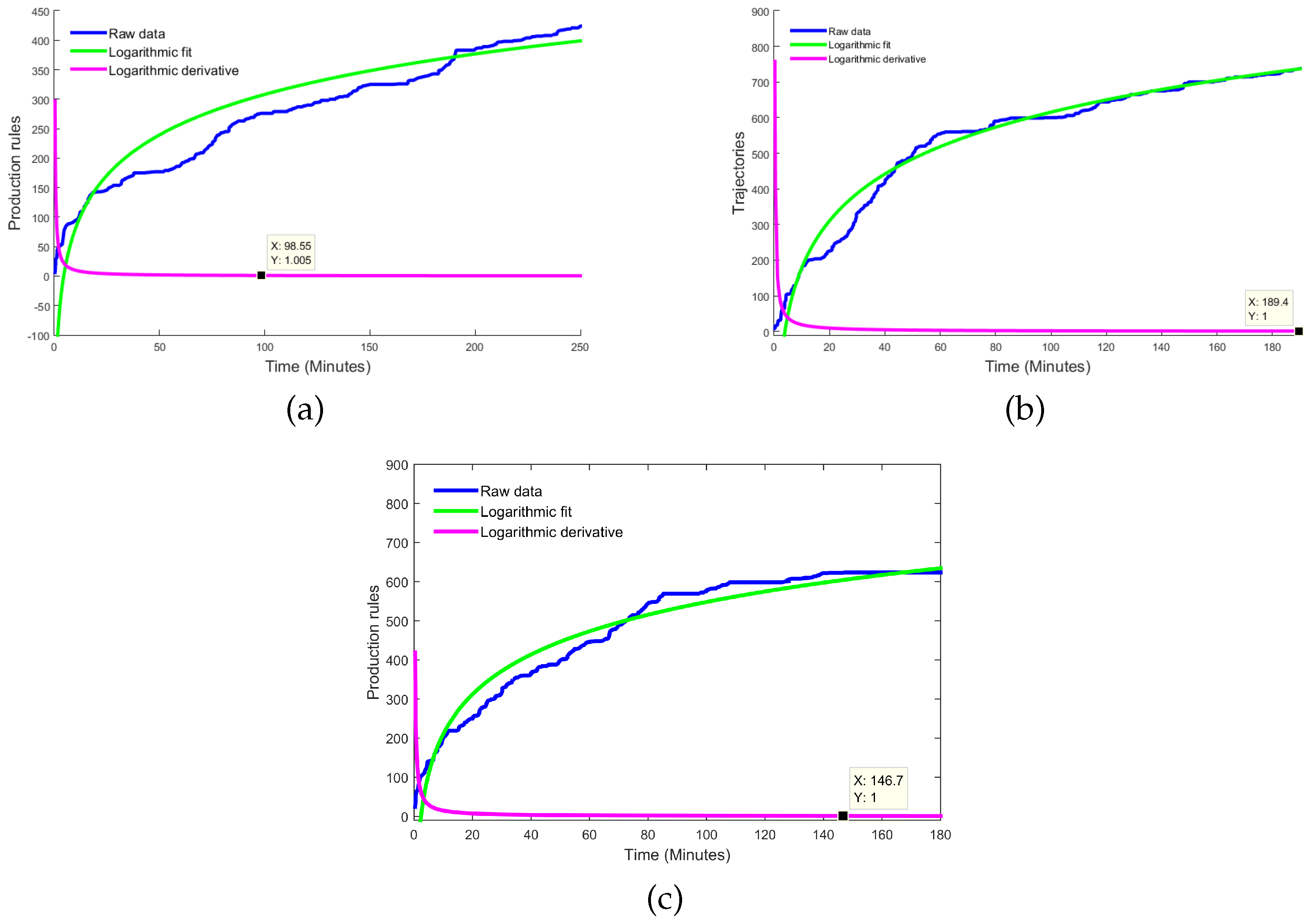
where the values of a and b in Equation (9) are obtained using the least squares technique [54], thereby determining the curve C, which shows the variation of . At this point, the central contribution of this work becomes clear, namely the criterion for information sufficiency, which can now be represented as:
Due to the nature of the logarithmic function, it is not possible to define the sufficiency criterion as , as this would cause an overfitting problem . The recommended value for the information sufficiency criterion is defined as for Equation (10). Given that the information entered into the system is , then when , we have , otherwise .
4. Experimental Analysis and Results
In this section, the proposal made in Section 2 and Section 3 is validated, obtaining video sequence information corresponding to three test scenarios. The first scenario corresponds to a PTZ camera capturing a side view of the analyzed scenario (scenario 1), while the second corresponds to a static 360° fisheye camera with a top view of the scenario (scenario 2). Finally, the third scenario (scenario 3) was obtained from an aerial shot using a wide-angle camera. These scenarios can be observed in Figure 3.
4.1. Experimental Process
To validate the proposal, we propose a process for automatically obtaining states of motion, which are directly related to . The proposed method consists of the following stages:
- 1.
- Obtaining trajectories. The trajectories of the movement observed in the scene represented by the set are obtained during the scene modeling process. This set contains multiple trajectories detected and enumerated incrementally, defined as . Each trajectory is composed of a sequence of positions , which describe the movement pattern associated with the intensity of pixel at position corresponding to the movement captured in the scene over time t.
- 2.
- Movement states definition. With the information on the movement of objects contained in , it is necessary to understand the dynamics of the objects in the scene over time. This temporal representation is achieved by the function , which relates the movement information of the trajectories to the membership of each pixel in the movement. By analyzing the belonging to the movement using , an accumulated surface is formed that contains the integrated information of the movement patterns. By applying the algorithm to , a two-dimensional representation of the regions with the highest probability of belonging to the movement is obtained, which are defined in the set of states E.
- 3.
- Symbol strings. At this stage, once the states E have been defined, the state mask is constructed, which relates each state to a symbol . The relationship between the movement positions and the states forms the state trajectories . Applying yields the symbolic sequences .
- 4.
- Sufficiency of information. The movement sequences are used to infer grammars by means of . This process generates a dictionary of production rules , where the change in the cardinality of the set of production rules is taken as a reference to define the criterion to define when the system has learned enough, shows the increase in the number of rules. Naturally, when analyzing the change in , we see that when meets the condition , this means that , therefore, no new production rule is being generated in the dictionary. This characteristic of the behavior of the function is a clear indication that a point of sufficiency of acquired information is being reached.
- 5.
- Dynamics modeling. Once sufficient information has been defined to model the scene, activities are detected by applying SEQUITUR to the movement sequences obtained.
4.2. Results
Information from the video sequences corresponding to the scenarios Figure 3, described below, is used. shows the interior of a laboratory with low light variability through a fixed camera with a resolution of pixels; captures the scene using a fish-eye camera under controlled lighting conditions with a resolution of pixels; and the third scenario , which acquires information on traffic flow at a roundabout using a drone with a resolution of pixels, where there is no control over the lighting.
Following the methodology proposed in the previous section Figure 2, the videos are analyzed in order to extract the movement patterns. With the information on the moving objects when applying Equation (3), it is possible to obtain the movement patterns , to determine the temporality of the movement , allowing the movement membership of each pixel to be visualized, as described in Equation (4).
Once the information on belonging to the movement has been obtained, it is easy to observe how the movement zones in the scene change with respect to time , which, when applying , shows that as time passes, the moving objects cover most of the areas of the scenes, a process that can be observed in Figure 5.
The information on the movement positions stored by each can be seen in the movement areas in Figure 4. It can be inferred that the information obtained in is related to a high degree of information about the movement of objects in the scene Figure 5.
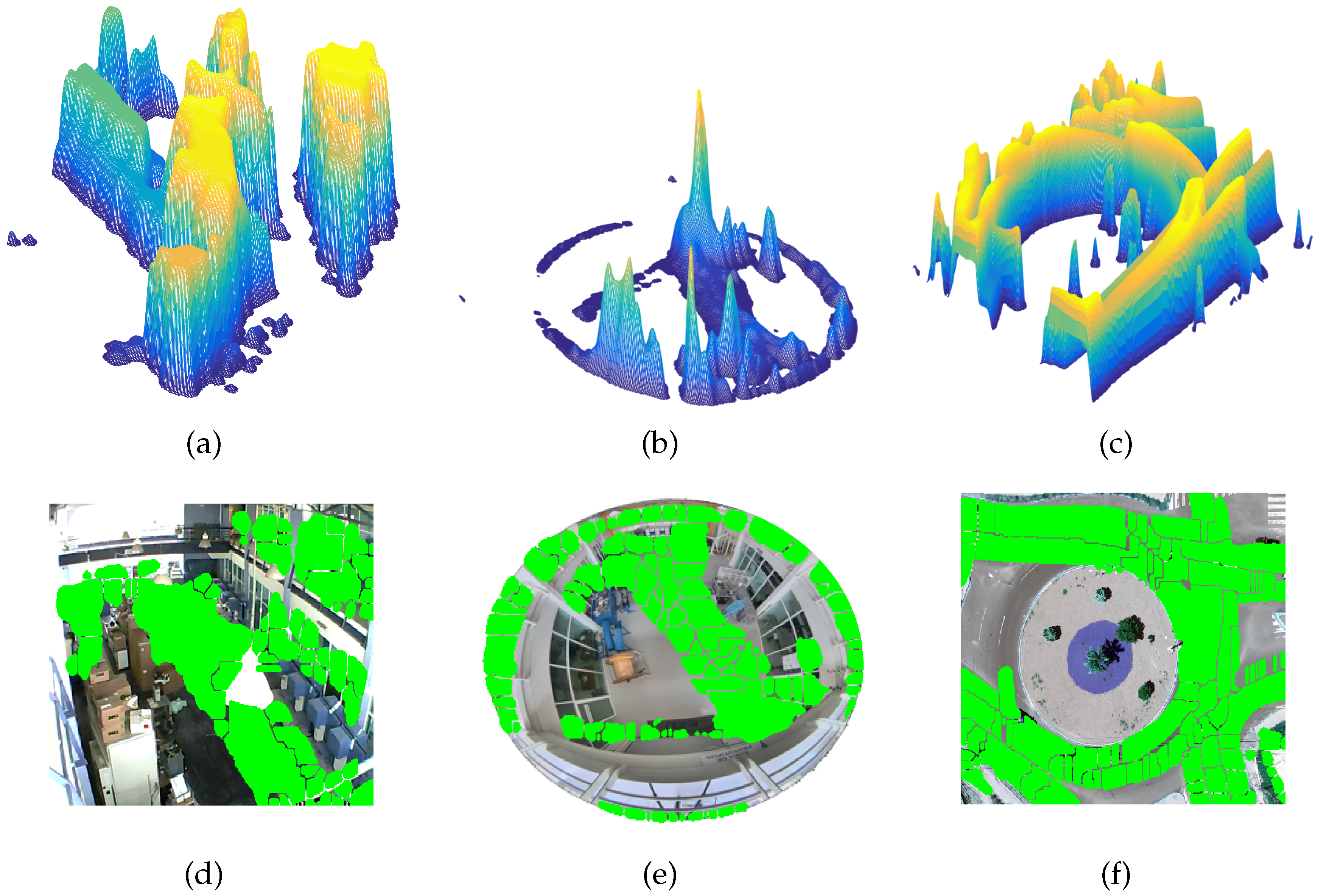
With the temporal representation of movement using the function , it is possible to observe how the information on movement patterns is distributed throughout the scene with for minutes. Al aplicar a la superficie acumulada se obtienen los estados E que representan las regiones donde existe mas probabilidad de pertenecia al movimiento, este proceso puede observarse en la siguiente Figure 6.
Figure 4.
Obtaining temporality of movement : (a) Detection of movement ; (b) Trajectory ; and (c) Temporality of movement of .
Figure 4.
Obtaining temporality of movement : (a) Detection of movement ; (b) Trajectory ; and (c) Temporality of movement of .
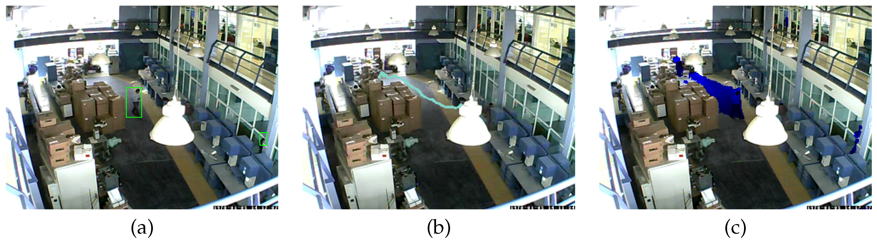
Figure 5.
Trajectories for the three scenarios, obtained at different time intervals t. (a),(b) and (c) Movement temporality for for t equal to 5 minutes.
Figure 5.
Trajectories for the three scenarios, obtained at different time intervals t. (a),(b) and (c) Movement temporality for for t equal to 5 minutes.
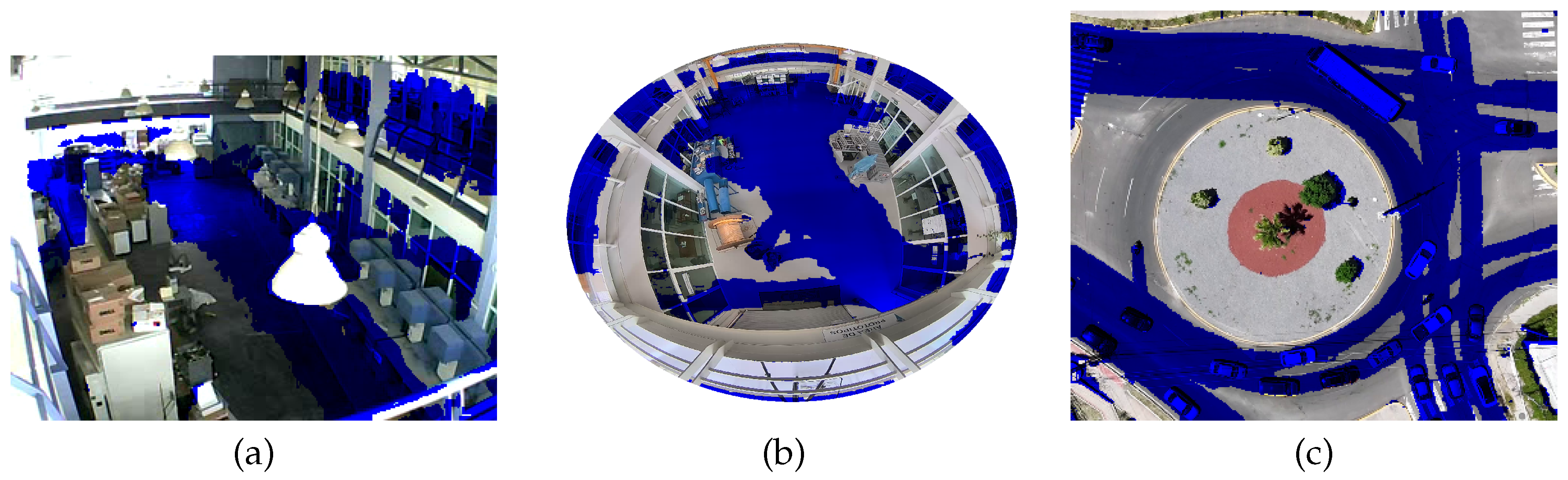
Figure 6.
Definition of states E for the three scenarios with minutes: (a-c) Surface with movement pattern information in scenarios , , and ; (d-f) State mask for the three scenarios.
Figure 6.
Definition of states E for the three scenarios with minutes: (a-c) Surface with movement pattern information in scenarios , , and ; (d-f) State mask for the three scenarios.
After defining each state within the scenarios and associating it with the corresponding trajectories, the trajectories are obtained. From this, it is possible to apply to obtain the symbolic representation of the movement patterns. In this process, each state is assigned a symbol . For this work, the symbols used are . The trajectory in Figure 7 (a) can now be represented as . This representation allows us to infer a grammar for this symbolic representation.
The relationship between the growth in the number of rules generated for the grammars inferred on the trajectories obtained in 5 minutes is shown in Figure 8. The incremental behavior in the number of production rules generated when inferring the grammars for the total trajectories obtained in the time defined as 5 minutes. Applying the same principle to Figure 7 (f), with the grammar , we observe that 14 new rules were generated corresponding to .
The relationship between trajectories and grammars can be seen in Figure 8, which shows the behavior of the production rules R for . The number of trajectories obtained over time is not related to the number of production rules generated to model the different trajectories .
This property allows us to begin the information sufficiency process, which consists of performing a classification described in Equation (7), where the objective of the process is to discriminate those trajectories that are not generating new information. Each rule that is added to the dictionary is selected by applying a similarity criterion or, when a trajectory does not generate new information, is satisfied, with the information from the trajectories that generate new rules that can be included in the dictionary it is possible to form a discrete function , which stores the cardinality of the dictionary with respect to time t. When graphing this discrete function , what can be observed is that as the information analysis time increases, the production rules comply more with , this can be seen in Figure 8.
The parts in red show the moments in time when no new information was generated, despite constantly obtaining movement information. This means that one trajectory shares information with another trajectory .
For this proposal, repetitiveness is an indicator that shows that the new movement information obtained from the scenario begins to lose significance . Up to this point, it is difficult to define a criterion for information sufficiency based on the number of repeated rules in the dictionary over time.
This leads to focusing efforts on approximating the discrete function with a continuous function . This approximation is possible by calculating the values a and b and substituting them into Equation (9), in order to obtain the continuous values of that best describe the growth curve of the production rules obtained over time in each of the scenarios. This process can be seen in Figure 10.
Taking advantage of the characteristics of the continuous function , we focus on analyzing how this function changes at points where there is high repetitiveness of production rules . Now it is possible to apply a criterion of information sufficiency based on the change in the approximate function Equation (10), which is defined as , where the function provides information on the growth of the production rules obtained over time. The minimum value of information desired to define that the new movement information obtained is significant is when at least one new production rule is being obtained. Then this criterion is passed to the definition of information sufficiency with value .
The sufficiency criterion is applied in the study scenarios in order to obtain the automatic definition of the movement information time necessary to determine that the information analyzed has been sufficient. For scenario 1, the time t associated with this criterion is minutes, and for scenario 2, the time minutes (see Figure 10).
Figure 9.
Relationship between the behavior of states , production rules, and trajectories, corresponding to minutes: (a, d, g) states ; (b, e, h) production rules ; and (c, f, i) generated trajectories S.
Figure 9.
Relationship between the behavior of states , production rules, and trajectories, corresponding to minutes: (a, d, g) states ; (b, e, h) production rules ; and (c, f, i) generated trajectories S.
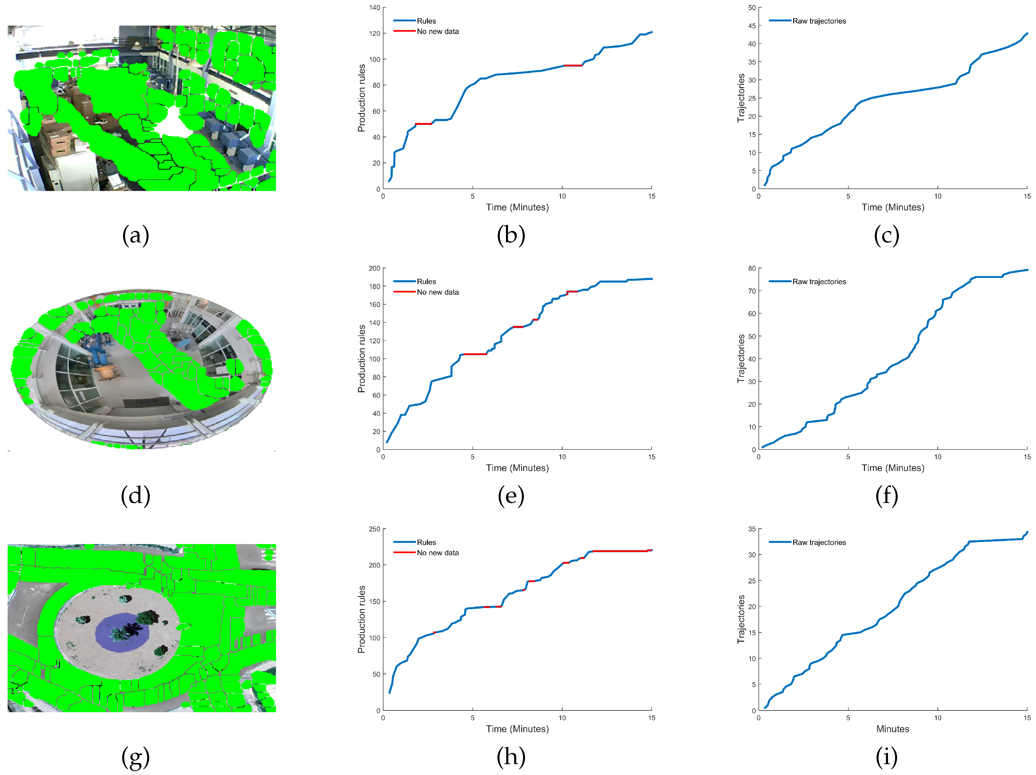
Figure 10.
Time required for sufficient movement information : (a) Scenario 1 minutes and ; (b) Scenario 2 minutes and ; (c) Scenario 3 minutes and .
Figure 10.
Time required for sufficient movement information : (a) Scenario 1 minutes and ; (b) Scenario 2 minutes and ; (c) Scenario 3 minutes and .
With the growth information in the dictionaries corresponding to the analyzed scenarios, this is directly associated with the time in each scenario. For the sufficiency of information, work is being done to generate more expressive trajectories, taking the information from the accumulated movement patterns and as shown in Figure 11.
The information from is used to form a new representation of the movement of type , with more expressive trajectories composed of the states of the scene where the movement is detected. With this information, it is possible to model the scene for activity detection. The information needed to train the model was defined by the criterion . In turn, the rules learned by the model and stored in the dictionary are validated to infer grammars and validate them against a new set of trajectories, thus determining the effectiveness of the model in each scenario.
The effectiveness of each model is presented in Table 3, where the results obtained in the three scenarios evaluated are compared. It can be seen that efficiency varies depending on the particular morphology of each scenario. This validation supports the proposal put forward in this work, demonstrating that the criterion of information sufficiency is capable of adapting to different contexts while maintaining consistent levels of performance.
5. Discussion and Conclusions
Learning algorithms are widely used today; however, like any process, they have areas for improvement and opportunities for optimization. One of the most relevant and widely studied areas today is the need for large volumes of information to train them properly. Obtaining this data can be complex and costly, both in terms of time and computational resources. In this regard, it is essential to have proposals such as the one presented in this paper, which introduces a new criterion for defining the sufficiency of information required in the learning of this type of algorithm. This section discusses the results obtained with the information sufficiency criterion, emphasizing the objectives achieved, the benefits obtained, and the limitations identified.
The application of the proposed method in the three scenarios evaluated proved to be an efficient tool for establishing a new criterion of information sufficiency, taking advantage of the relationship between the grammatical rules generated by the model and the dynamics of the objects in the analyzed scene. The Section 4, dedicated to experimentation, presents the results of trajectory modeling using grammars in three different scenarios. These results, summarized in Table 3, show the analysis of the model in each case.
In the first scenario, captured with a PTZ camera, the model indicated that a training time of minutes was sufficient for the generated data to achieve a high degree of repeatability, thus allowing the training time to be automatically determined. The resulting rule set contained rules, achieving an accuracy of when validated with new trajectories. In the second scenario, recorded with a 360° fisheye camera, the model determined a training time of minutes, resulting in a rule set of rules and an accuracy of . Finally, in the third scenario, captured with a wide-angle camera, the estimated training time was minutes, with a rule set of rules and a validation accuracy of . These results can be seen in more detail in Table 3.
Regarding the limitations of this approach, it should be noted that the method assumes that objects move freely within the scene and that, given sufficient time, all areas will be covered by motion data. This assumption may not hold true in scenarios where movement is restricted or the areas of movement are limited.
Furthermore, the results obtained in the analyzed scenarios may vary when applied to different environments. The intrinsic parameters of the model are not fully generalized, which could affect the method’s effectiveness in contexts with different characteristics.
In conclusion, this work presents an effective approach for defining a criterion for information sufficiency. The main advantage lies in representing trajectories as sequences of symbols , which allows us to infer a grammar to model the dynamics of the objects. This results in rules where, if two trajectories exhibit similarities, it means that at least one production rule applies to a portion of both trajectories, thus significantly reducing the amount of information needed to represent the movement. In this way, the trajectory information becomes more expressive and suitable for modeling and machine learning purposes.
5.1. Further Works
The information sufficiency criterion developed in this work opens up a wide range of avenues for future research. One initial direction is the application of this criterion to the modeling of stochastic processes, particularly to Hidden Markov Models (HMM). In this context, the regions that form the trajectories can be directly mapped to the visible states of an HMM. This correspondence offers a significant advantage: it ensures that the number of visible states is determined by the information sufficiency, thus avoiding both overfitting and under-representation of the underlying dynamics. Furthermore, the grammatical structure can serve as a guide for estimating the transition and emission probabilities, providing an additional layer of regularization during HMM training.
Finally, this approach can be extended to other domains where symbolic representation of data is useful, such as multivariate time series analysis, pattern recognition in biological sequences, or predicting behavior in complex environments. In all these cases, the grammar induced from the data, along with the concept of information sufficiency, could contribute to improving the generalization ability of models and reducing training costs.
Author Contributions
Conceptualization, H.H.-R. and H.J.-H.; Formal analysis, A.-M.H.-N.,D.C.-E. and H.J.-H.; Methodology, H.H.-R., A.-M.H.-N. and H.J.-H.; Software, H.J.-H.; Supervision, H.H-R., D.C.-E. and H.J.-H.; Writing—original draft, J.-L.P.-R. and A.-M.H.-N.; Writing—review and editing, H.J.-H., J.-L.P.-R. and H.H.-R.. All authors have read and agreed to the published version of the manuscript.
Funding
This research received no external funding.
Institutional Review Board Statement
Not applicable.
Data Availability Statement
The data availability in this study is on request from the corresponding author.
Acknowledgments
We wish to give thanks to CIDESI, CONAHCYT, and the Mexican Artificial Intelligence Alliance, with the FORDECYT Project 296737 Consorcio en Inteligencia Artificial which provided the student scholarships and CIICCTE (Centro de Investigación e Innovación en Ciencias de la Computación y Tecnología Educativa) which provided technical and infrastructure support.
Conflicts of Interest
The authors declare no conflicts of interest.
Abbreviations
The following abbreviations are used in this manuscript:
| CNN | Convolutional Neural Network |
| HMM | Hidden Markov Models |
| KNN | K-nearest neighbors |
| PTZ | Pan, Tilt, and Zoom |
References
- Fedorov, A.; Nikolskaia, K.; Ivanov, S.; Shepelev, V.; Minbaleev, A. Traffic flow estimation with data from a video surveillance camera. Journal of Big Data 2019, 6, 1–15. [Google Scholar] [CrossRef]
- Elharrouss, O.; Almaadeed, N.; Al-Maadeed, S. A review of video surveillance systems. Journal of Visual Communication and Image Representation 2021, 77, 103116. [Google Scholar] [CrossRef]
- Ess, A.; Leibe, B.; Schindler, K.; Van Gool, L. A mobile vision system for robust multi-person tracking. In Proceedings of the 2008 IEEE conference on computer vision and pattern recognition. IEEE, 2008, pp. 1–8. [CrossRef]
- Mabrouk, A.B.; Zagrouba, E. Abnormal behavior recognition for intelligent video surveillance systems: A review. Expert Systems with Applications 2018, 91, 480–491. [Google Scholar] [CrossRef]
- Sultani, W.; Chen, C.; Shah, M. Real-world anomaly detection in surveillance videos. In Proceedings of the Proceedings of the IEEE conference on computer vision and pattern recognition, 2018, pp. 6479–6488. [CrossRef]
- Wibowo, M.E.; Ashari, A.; Putra, M.P.K.; et al. Improvement of Deep Learning-based Human Detection using Dynamic Thresholding for Intelligent Surveillance System. International Journal of Advanced Computer Science and Applications 2021, 12. [Google Scholar] [CrossRef]
- Sreenu, G.; Durai, S. Intelligent video surveillance: a review through deep learning techniques for crowd analysis. Journal of Big Data 2019, 6, 1–27. [Google Scholar] [CrossRef]
- Luck, S.J.; Stewart, A.X.; Simmons, A.M.; Rhemtulla, M. Standardized measurement error: A universal metric of data quality for averaged event-related potentials. Psychophysiology 2021, 58, e13793. [Google Scholar] [CrossRef]
- Roh, Y.; Heo, G.; Whang, S.E. A survey on data collection for machine learning: a big data-ai integration perspective. IEEE Transactions on Knowledge and Data Engineering 2019, 33, 1328–1347. [Google Scholar] [CrossRef]
- Rijali, A. Analisis data kualitatif. Alhadharah: Jurnal Ilmu Dakwah 2018, 17, 81–95. [Google Scholar] [CrossRef]
- Denes, G.; Jindal, A.; Mikhailiuk, A.; Mantiuk, R.K. A perceptual model of motion quality for rendering with adaptive refresh-rate and resolution. ACM Transactions on Graphics (TOG) 2020, 39, 133:1–133:17. [Google Scholar] [CrossRef]
- He, Y.; Wei, X.; Hong, X.; Shi, W.; Gong, Y. Multi-target multi-camera tracking by tracklet-to-target assignment. IEEE Transactions on Image Processing 2020, 29, 5191–5205. [Google Scholar] [CrossRef]
- Gilroy, S.; Jones, E.; Glavin, M. Overcoming occlusion in the automotive environment—A review. IEEE Transactions on Intelligent Transportation Systems 2019, 22, 23–35. [Google Scholar] [CrossRef]
- Wang, A.; Sun, Y.; Kortylewski, A.; Yuille, A.L. Robust object detection under occlusion with context-aware compositionalnets. In Proceedings of the Proceedings of the IEEE/CVF conference on computer vision and pattern recognition, 2020, pp. 12645–12654. [CrossRef]
- Li, H.; Chen, G.; Li, G.; Yu, Y. Motion guided attention for video salient object detection. In Proceedings of the Proceedings of the IEEE/CVF international conference on computer vision, 2019, pp. 7274–7283. [CrossRef]
- Zhu, Y.; Newsam, S. Motion-aware feature for improved video anomaly detection. arXiv preprint arXiv:1907.10211 2019. [CrossRef]
- Griffin, B.A.; Corso, J.J. Depth from camera motion and object detection. In Proceedings of the Proceedings of the IEEE/CVF Conference on Computer Vision and Pattern Recognition, 2021, pp. 1397–1406. [CrossRef]
- Jain, J.; Singh, A.; Orlov, N.; Huang, Z.; Li, J.; Walton, S.; Shi, H. Semask: Semantically masked transformers for semantic segmentation. In Proceedings of the Proceedings of the IEEE/CVF International Conference on Computer Vision, 2023, pp. 752–761. [CrossRef]
- Sun, Z.W.; Hua, Z.X.; Li, H.C.; Zhong, H.Y. Flying Bird Object Detection Algorithm in Surveillance Video Based on Motion Information. IEEE Transactions on Instrumentation and Measurement 2024, 73, 1–15. [Google Scholar] [CrossRef]
- Dong, G.; Zhao, C.; Pan, X.; Basu, A. Learning Temporal Distribution and Spatial Correlation Toward Universal Moving Object Segmentation. IEEE Transactions on Image Processing 2024, 33, 2447–2461. [Google Scholar] [CrossRef]
- Zhang, T.; Huang, B.; Wang, Y. Object-occluded human shape and pose estimation from a single color image. In Proceedings of the Proceedings of the IEEE/CVF conference on computer vision and pattern recognition, 2020, pp. 7376–7385. [CrossRef]
- Liu, D.; Li, Y.; Lin, J.; Li, H.; Wu, F. Deep learning-based video coding: A review and a case study. ACM Computing Surveys (CSUR) 2020, 53, 1–35. [Google Scholar] [CrossRef]
- Vu, H.N.; Nguyen, M.H.; Pham, C. Masked face recognition with convolutional neural networks and local binary patterns. Applied Intelligence 2022, 52, 5497–5512. [Google Scholar] [CrossRef]
- Meinhardt, T.; Kirillov, A.; Leal-Taixe, L.; Feichtenhofer, C. Trackformer: Multi-object tracking with transformers. In Proceedings of the Proceedings of the IEEE/CVF conference on computer vision and pattern recognition, 2022, pp. 8844–8854. [CrossRef]
- Kumar, S.; Yadav, J.S. Video object extraction and its tracking using background subtraction in complex environments. Perspectives in Science 2016, 8, 317–322, Recent Trends in Engineering and Material Sciences. [Google Scholar] [CrossRef]
- Pandey, S.; Jain, P.; Patel, P. Video Background Subtraction Algorithms for Object Tracking. In Proceedings of the 2022 Third International Conference on Intelligent Computing Instrumentation and Control Technologies (ICICICT), 2022, pp. 464–469. [CrossRef]
- Chen, X.; Williams, B.M.; Vallabhaneni, S.R.; Czanner, G.; Williams, R.; Zheng, Y. Learning active contour models for medical image segmentation. In Proceedings of the Proceedings of the IEEE/CVF conference on computer vision and pattern recognition, 2019, pp. 11632–11640. [CrossRef]
- Li, L.; Zhou, T.; Wang, W.; Li, J.; Yang, Y. Deep hierarchical semantic segmentation. In Proceedings of the Proceedings of the IEEE/CVF Conference on Computer Vision and Pattern Recognition, 2022, pp. 1246–1257. [CrossRef]
- Tao, A.; Sapra, K.; Catanzaro, B. Hierarchical multi-scale attention for semantic segmentation. arXiv preprint arXiv:2005.10821 2020. [CrossRef]
- Wu, L.; Wang, Q.; Jian, M.; Zhao, Y.Q.B. A Comprehensive Review of Group Activity Recognition in Videos. International Journal of Automation and Computing 2021, 17. [Google Scholar] [CrossRef]
- A. Yilmaz, O.J.; Shah, M. Object tracking: a Survey. ACM Computing surveys 2006, 38, 13. [Google Scholar] [CrossRef]
- Daldoss, M.; Piotto, N.; Conci, N.; De Natale, F.G. Learning and matching human activities using regular expressions. In Proceedings of the 2010 IEEE International Conference on Image Processing. IEEE, 2010, pp. 4681–4684. [CrossRef]
- Li, D.; Wu, M. Pattern recognition receptors in health and diseases. Signal transduction and targeted therapy 2021, 6, 291. [Google Scholar] [CrossRef]
- Braga-Neto, U. Fundamentals of pattern recognition and machine learning; Springer, 2020. [CrossRef]
- Emmanuel, T.; Maupong, T.; Mpoeleng, D.; Semong, T.; Mphago, B.; Tabona, O. A survey on missing data in machine learning. Journal of Big data 2021, 8, 1–37. [Google Scholar] [CrossRef]
- Callaghan, M.W.; Müller-Hansen, F. Statistical stopping criteria for automated screening in systematic reviews. Systematic Reviews 2020, 9, 1–14. [Google Scholar] [CrossRef]
- Nevill-Manning, C.G.; Witten, I.H. Identifying hierarchical structure in sequences: A linear-time algorithm. Journal of Artificial Intelligence Research 1997, 7, 67–82. [Google Scholar] [CrossRef]
- Mitarai, S.; Hirao, M.; Matsumoto, T.; Shinohara, A.; Takeda, M.; Arikawa, S. Compressed pattern matching for SEQUITUR. In Proceedings of the Proceedings DCC 2001. Data Compression Conference. IEEE, 2001, pp. 469–478. [CrossRef]
- A. A. Sekh.; D.P. Dogra.; S. Kar.; P.P. Roy. Video trajectory analysis using unsupervised clustering and multi-criteria ranking. Soft Computing 2020, 24, 16643–16654. [Google Scholar] [CrossRef]
- Rao, S.; Sastry, P.S. Abnormal activity detection in video sequences using learnt probability densities. In Proceedings of the TENCON 2003. Conference on Convergent Technologies for Asia-Pacific Region, 2003, Vol. 1, pp. 369–372 Vol.1. [CrossRef]
- Guo, D.; Wu, E.Q.; Wu, Y.; Zhang, J.; Law, R.; Lin, Y. FlightBERT: binary encoding representation for flight trajectory prediction. IEEE Transactions on Intelligent Transportation Systems 2022, 24, 1828–1842. [Google Scholar] [CrossRef]
- Zhou, B.; Wang, Y.; Yu, G.; Wu, X. A lane-change trajectory model from drivers’ vision view. Transportation Research Part C: Emerging Technologies 2017, 85, 609–627. [Google Scholar] [CrossRef]
- Gamba, P.; Mecocci, A. Perceptual grouping for symbol chain tracking in digitized topographic maps. Pattern Recognition Letters 1999, 20, 355–365. [Google Scholar] [CrossRef]
- García-Huerta, J.M.; Jiménez-Hernández, H.; Herrera-Navarro, A.M.; Hernández-Díaz, T.; Terol-Villalobos, I. Modelling dynamics with context-free grammars. Video Surveill. Transp. Imaging Appl. 2014 2014, 9026, 6. [Google Scholar] [CrossRef]
- Rosani, A.; Conci, N.; Natale, F.G.D. Human behavior recognition using a context-free grammar. Journal of Electronic Imaging 2014, 23, 033016. [Google Scholar] [CrossRef]
- Hugo, J.H.; Jose-Joel, G.B.; Teresa, G.R. Detecting abnormal vehicular dynamics at intersections based on an unsupervised learning approach and a stochastic model. Sensors 2010, 10, 7576–7601. [Google Scholar] [CrossRef]
- Xue, Y.; Zhao, J.; Zhang, M. A watershed-segmentation-based improved algorithm for extracting cultivated land boundaries. Remote Sensing 2021, 13, 939. [Google Scholar] [CrossRef]
- Zhang, H.; Tang, Z.; Xie, Y.; Gao, X.; Chen, Q. A watershed segmentation algorithm based on an optimal marker for bubble size measurement. Measurement 2019, 138, 182–193. [Google Scholar] [CrossRef]
- Venu, D.; Kumar, A.A. Comparison of Traditional Method with watershed threshold segmentation Technique. The International journal of analytical and experimental modal analysis 2021, 13, 181–187. [Google Scholar]
- de la Higuera, C. Grammatical inference: learning automata and grammars. In Proceedings of the Cambridge University Press, 2010, pp. 1–502. [CrossRef]
- Nevill-Manning, C.G.; Witten, I.H. Compression and Explanation using Hierarchical Grammars. The Computer Journal 1997, 40, 103–116. [Google Scholar] [CrossRef]
- Åke Björck. Least Square Method; Vol. 1, Handbook of Numerical Analysis, Elsevier, 1990; pp. 465–652. [CrossRef]
- Gomila, R. Logistic or linear? Estimating causal effects of experimental treatments on binary outcomes using regression analysis. Journal of Experimental Psychology: General 2021, 150, 700. [Google Scholar] [CrossRef] [PubMed]
- Björck, Å. Numerical methods for least squares problems; SIAM, 2024. [CrossRef]
Figure 1.
Process for generating path trajectories: (a) Trajectory motion information , (b) Surface generated with trajectory information , and (c) States mask .
Figure 1.
Process for generating path trajectories: (a) Trajectory motion information , (b) Surface generated with trajectory information , and (c) States mask .
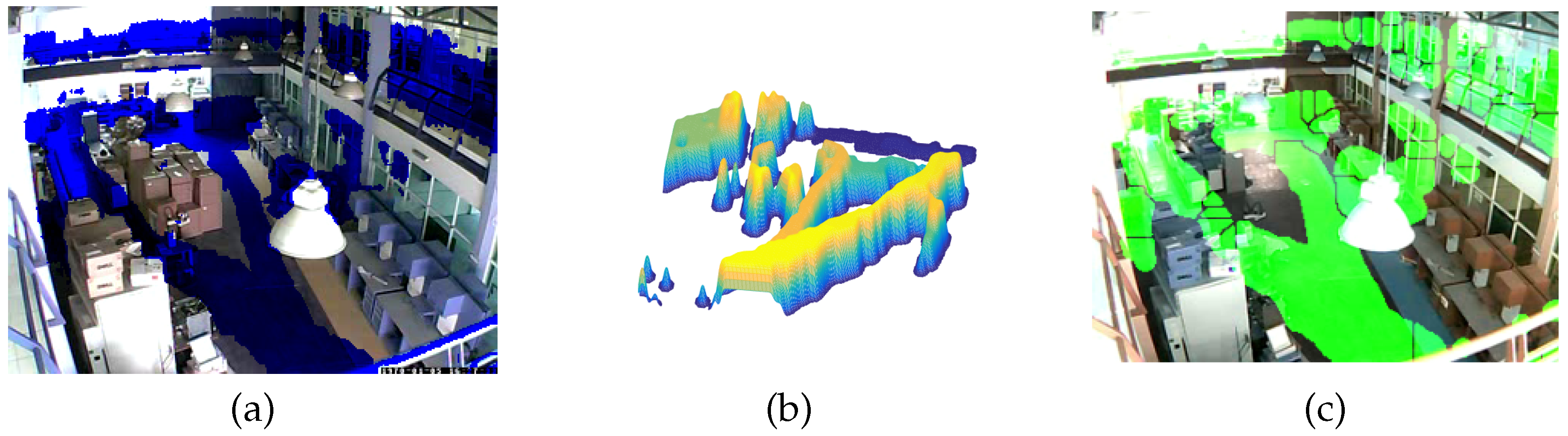
Figure 2.
Automatic selection process for rules generated.
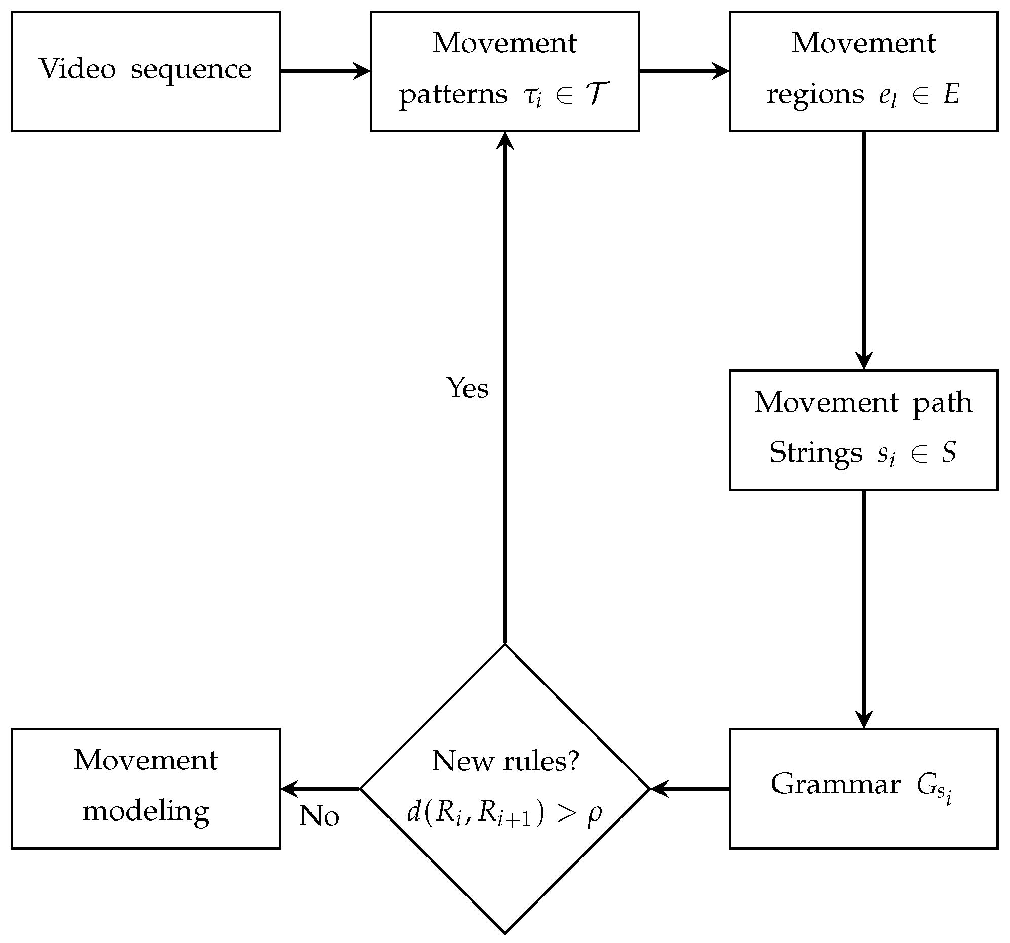
Figure 3.
Scenarios used to validate the proposal: (a) ; (b) and (c) .
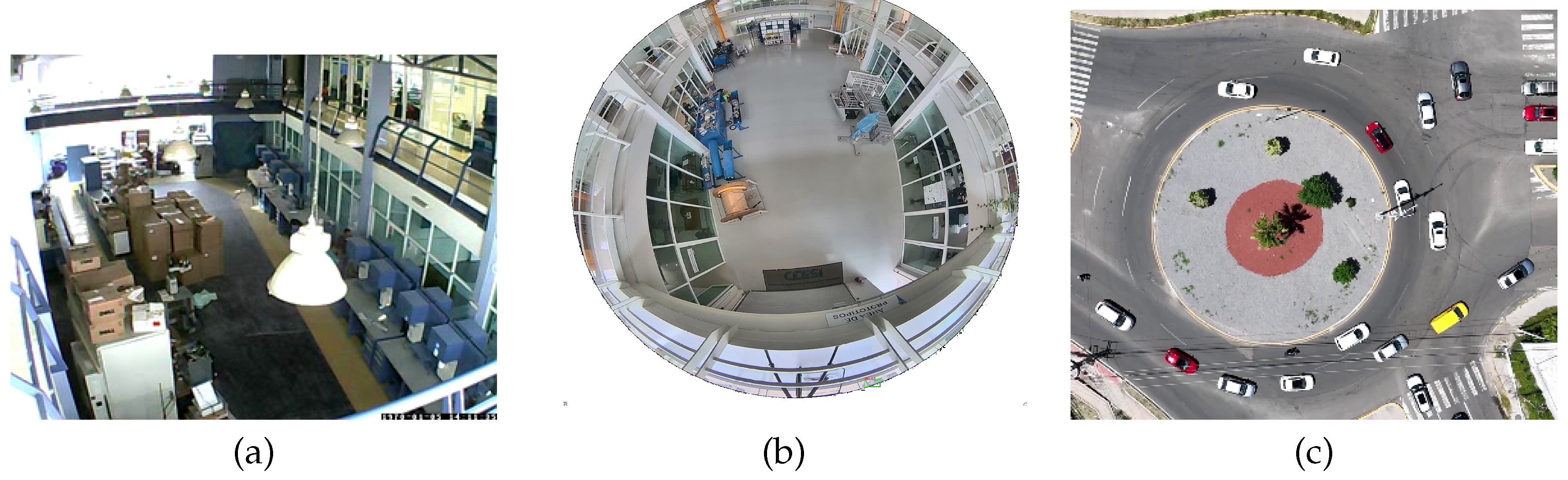
Figure 7.
Trajectories in their representations and : (a) Trajectory for scenario ; (b) Trajectory for scenario ; (c) Trajectory for scenario ; (d) Trajectory for scenario ; (e) Trajectory for scenario ; and (f) Trajectory for scenario .
Figure 7.
Trajectories in their representations and : (a) Trajectory for scenario ; (b) Trajectory for scenario ; (c) Trajectory for scenario ; (d) Trajectory for scenario ; (e) Trajectory for scenario ; and (f) Trajectory for scenario .
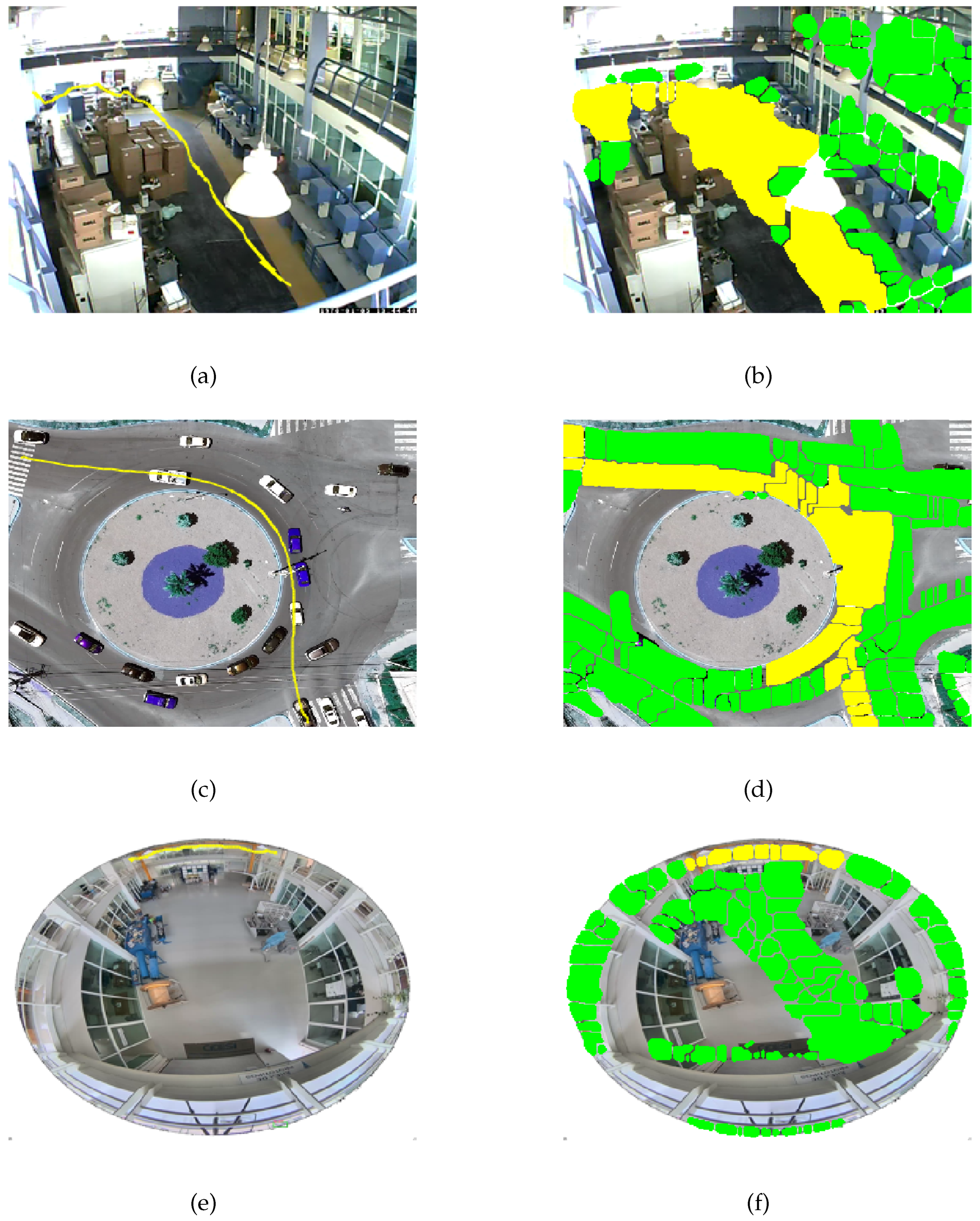
Figure 8.
Relationship between the number of production rules vs. trajectories with minutes: (a) Production rules for scenario and (b) behavior of the number of trajectories over time t for the first scenario.
Figure 8.
Relationship between the number of production rules vs. trajectories with minutes: (a) Production rules for scenario and (b) behavior of the number of trajectories over time t for the first scenario.
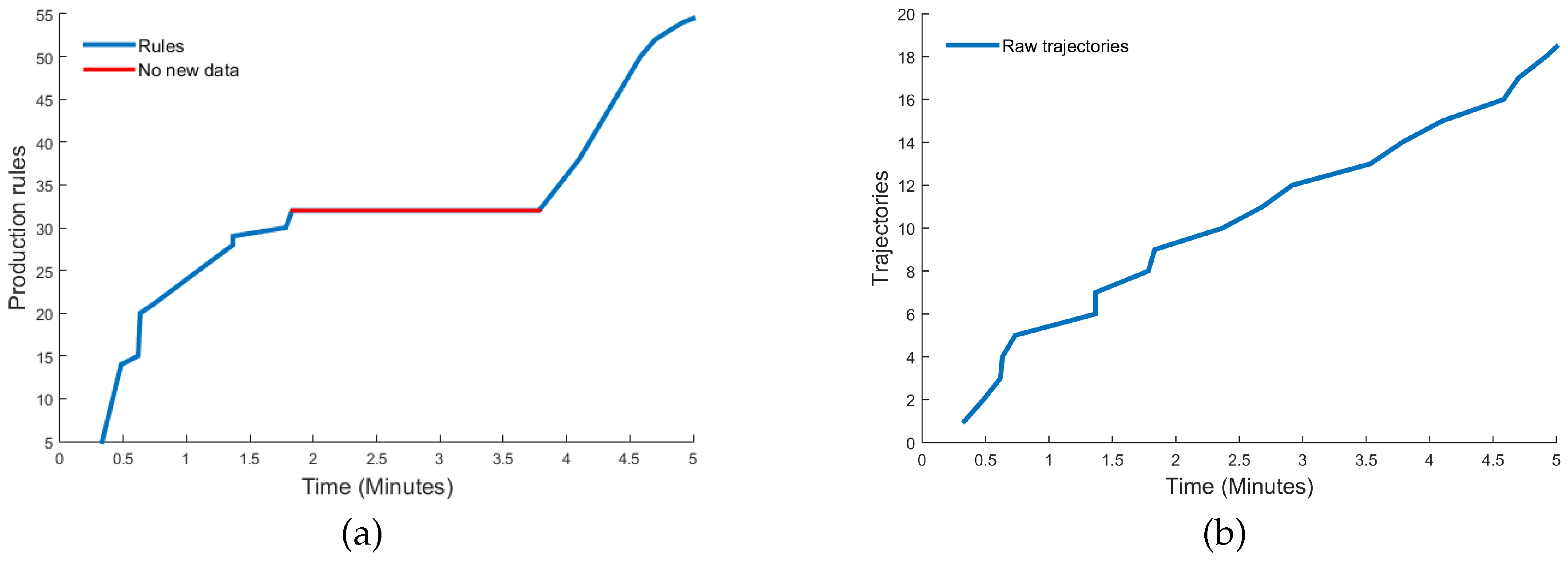
Figure 11.
Membership in the movement with (a) Movement information for ; (b) for ; (c) for ; (d) Surface generated with and (e) and (f) .
Figure 11.
Membership in the movement with (a) Movement information for ; (b) for ; (c) for ; (d) Surface generated with and (e) and (f) .
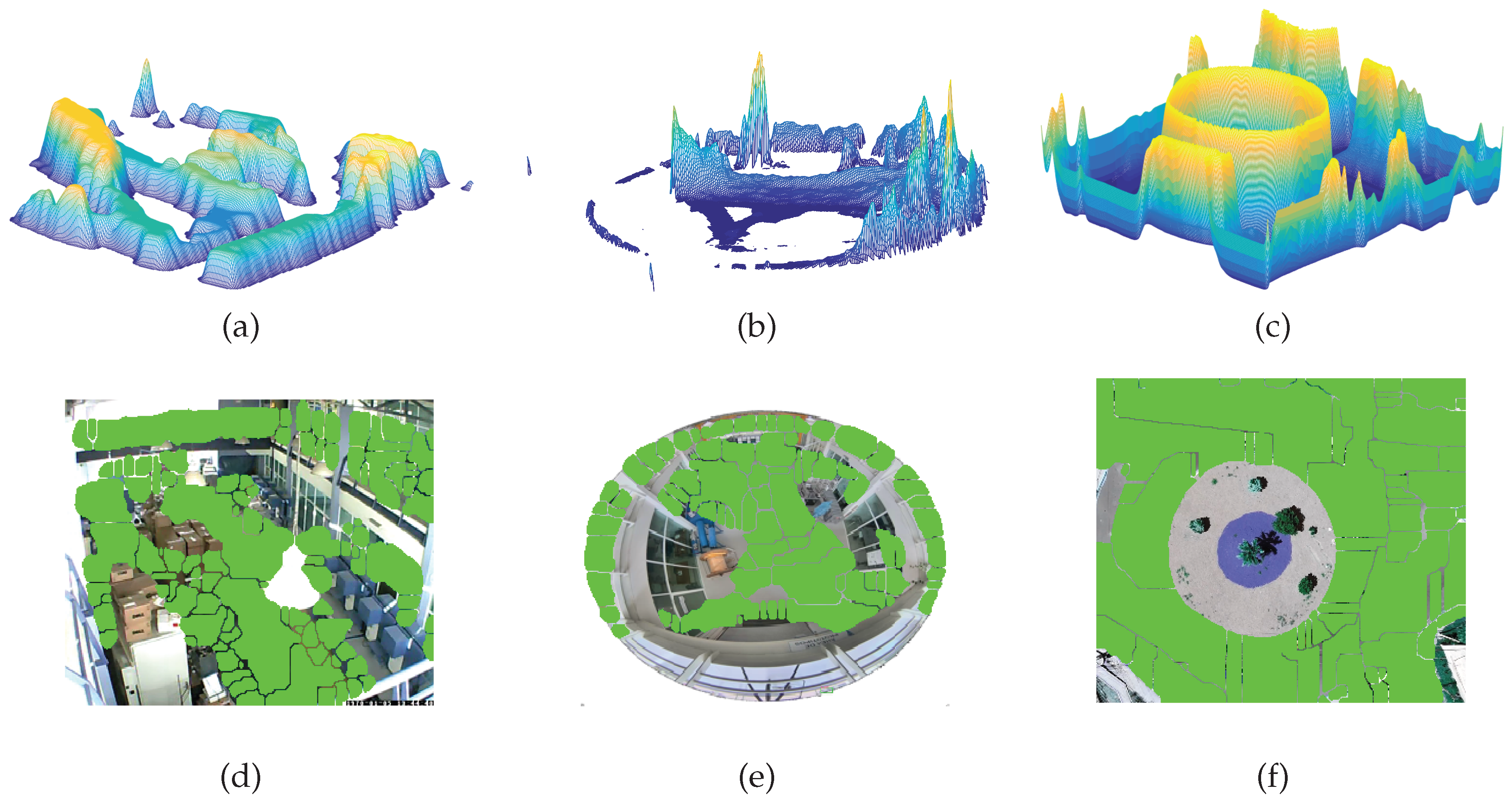

Table 1.
Comparison of movement coding techniques in similar context applications.
| Author | Motion Coding | State Definition | Remarks |
|---|---|---|---|
| Andrea Rosani et al. [45] | Hot spots | Empirical approach | The approach focuses on activity recognition for behavioral analysis in known scenarios using context-free grammars. By incorporating both positive and negative sampling, this method enhances discrimination capabilities during the retraining process, enabling better adaptation to environmental changes. |
| Garcia-Huerta et al. [44] | Labeled regions | Manual | The study focuses on detecting abnormal visual events within a scenario. Motion detection is achieved through temporal differences, applied as a decay function, which identifies motion zones. These zones are subsequently segmented using the Watershed transform. |
| Waqas Sultani et al. [5] | Labeled regions | Fixed number | This work proposes an anomaly detection model based on deep multiple instance learning. The model utilizes a fixed number of segments from both anomalous and normal surveillance videos. |
| M. Daldoss et al. [32] | Hot spots | Automatic | Introduces a method for analyzing trajectories by tracking objects through a two-view camera system in surveillance videos using automatically learned context-free grammars. The model is trained on a set of sequences that define rules for different behaviors. |
| Hernandez-Ramirez et al. (proposed) | Labeled regions | Automatic | This work introduces an approach centered on information sufficiency, where symbolic trajectories from object–labeled region interactions are used to infer grammars. The sufficiency criterion, defined by the stabilization of production rules, ensures a meaningful representation of scene dynamics. |
Table 2.
Process for generating grammars with SEQUITUR.
| Input | String | Grammar | Rules |
|---|---|---|---|
| a | |||
| b |
|
||
| d | |||
| a | |||
| b |
|
||
| c |
|
Table 3.
Results of trajectory experimentation in three different scenarios.
| Scenarios | Training time | Total trajectories | Dictionary rules | Accuracy (%) |
|---|---|---|---|---|
| (1) PTZ Camera | 98.55 minutes | 440 | 250 | 84.13 % |
| (2) Fisheye 360° Camera | 189.4 minutes | 1022 | 700 | 83.56 % |
| (3) Wide angle Camera | 146.7 minutes | 319 | 622 | 95.92 % |
Disclaimer/Publisher’s Note: The statements, opinions and data contained in all publications are solely those of the individual author(s) and contributor(s) and not of MDPI and/or the editor(s). MDPI and/or the editor(s) disclaim responsibility for any injury to people or property resulting from any ideas, methods, instructions or products referred to in the content. |
© 2025 by the authors. Licensee MDPI, Basel, Switzerland. This article is an open access article distributed under the terms and conditions of the Creative Commons Attribution (CC BY) license (http://creativecommons.org/licenses/by/4.0/).
Copyright: This open access article is published under a Creative Commons CC BY 4.0 license, which permit the free download, distribution, and reuse, provided that the author and preprint are cited in any reuse.


