Submitted:
03 October 2025
Posted:
03 October 2025
You are already at the latest version
Abstract
We study a stochastic differential model for the dynamics of institutional corruption, extending a deterministic three-variable system -corruption perception, proportion of sanctioned acts, and policy laxity- by incorporating Gaussian perturbations into key parameters. We prove global existence and uniqueness of solutions in the physically relevant domain, and we analyze the linearization around the asymptotically stable equilibrium of the deterministic system. Explicit mean-square bounds for the linearized process are derived in terms of the spectral properties of a symmetric matrix, providing insight into the temporal validity of the linear approximation. To investigate global behavior, we relate the first exit time from the domain of interest to backward Kolmogorov equations and solve the associated elliptic and parabolic PDEs numerically with FreeFEM, obtaining estimates of expectations and survival probabilities. An application to the case of Mexico highlights nontrivial effects: while the spectral structure governs local stability, institutional volatility can nonmonotonically accelerate global exit, showing that highly reactive interventions without effective sanctions increase uncertainty. Policy implications and possible extensions are discussed.
Keywords:
stochastic models
; spectral bounds
; exit times
; corruption models
MSC: 26A33; 49J20; 35R11; 49J15
1. Introduction
Institutional corruption, understood as the abuse of public power for private benefit, represents a critical obstacle to socioeconomic development and a threat to democratic governance. In recent years, it has been recognized that stochastic mathematical models—particularly those inspired by epidemic dynamics (SIR-type models)—offer a promising framework to analyze the spread of corruption and to evaluate the impact of anti-corruption policies; see, for example, [1,2,3,4]. These models often incorporate random factors (Brownian or Lévy noise) that capture intrinsic uncertainties, such as the random detection of offenses or variability in the effectiveness of sanctions. The stochastic formulation allows, among other things, the quantification of exit times (i.e., the first hitting times of acceptable corruption levels) via Kolmogorov/Fokker–Planck type partial differential equations, which are essential to assess the temporal effectiveness of governmental interventions.
In this work, we introduce a novel stochastic model for institutional corruption aimed at evaluating public policies. We start from a framework that explicitly includes policy-related variables such as investment in transparency, ethical education, and legal sanctions. By incorporating Brownian noise into the transition rates, we capture unpredictable variability in the effectiveness of such measures and in the spread of corrupt behavior. Mathematically, this leads to a system of multivariate stochastic differential equations (SDEs). A distinctive feature of our model is the emphasis on exit times of corruption under different policy scenarios. We define a domain of interest D (for instance, high levels of corruption) and compute the first exit time to more acceptable levels. The distribution and density of are obtained analytically from the Kolmogorov/Fokker–Planck equation, whose numerical solution is computed using FreeFEM. This enables, for example, the evaluation of how changes in audit funding or educational campaigns affect the expected time to achieve a “reduction” of corruption.
The proposed formulation addresses several issues identified in the literature, see [14]. First, it explicitly integrates public policy factors into the stochastic dynamics, thereby connecting model parameters to real interventions. Second, by focusing on exit times, it provides a clear temporal metric (rather than purely population-based measures) to assess policy efficiency. Finally, it employs robust numerical methods to solve the PDEs associated with the exit time .
A central theoretical result of this work arises from the study of the linearization of the system around the deterministic equilibrium. We show that bounds on the second-order moment (the mean square of perturbations) are governed by the spectral structure of the linearized matrix—that is, by its eigenvalues rather than by the magnitude of a single noise term. In particular, the presence of a dominant positive eigenvalue leads to exponential growth of variability and limits the temporal validity of any linear approximation, rendering its conclusions essentially local in time. Conceptually, this explains why small variations in institutional reactivity parameters or in the effectiveness of sanctions can amplify uncertainty in non-intuitive ways, producing “overcorrection” effects. From a public policy perspective, this suggests that interventions must be designed with the collective interaction of parameters in mind (i.e., the system’s spectral structure), rather than focusing solely on reducing volatility in a single component.
We apply the proposed framework to the case of Mexico and compute exit times numerically for different policy calibrations. The results show that persistence in undesirable states does not depend on a single parameter in isolation but rather on the interaction between institutional laxity, punishment effectiveness, and governmental reactivity: certain combinations can significantly prolong high levels of corruption. Moreover, the volatility of institutional laxity affects exit speed in a non-monotone way: reducing policy uncertainty often accelerates recovery, but excessively reactive responses without effective sanctions may induce overcorrections and increase uncertainty. Based on our analysis for Mexico, we recommend prioritizing interventions that modify the system’s drift (e.g., strengthening the effectiveness of sanctions and implementing institutional reforms that reduce regulatory laxity), rather than relying on random fluctuations; in addition, institutional responses should be graduated to avoid overcorrections that exacerbate uncertainty. It is essential to incorporate time-based metrics derived from exit times to establish realistic policy horizons and evaluation criteria, thereby identifying high-risk parameter combinations. Such measures allow for faster and more robust improvements in reducing corruption while minimizing unpredictable effects stemming from complex interactions among laxity, sanction, and reactivity.
The organization of the paper is as follows. In Section 2, we present the deterministic model introduced in [14], which we then perturb randomly. Section 3 introduces the stochastic dynamics and establishes global existence. Section 4 studies a linear approximation of the stochastic system. Section 5 and Section 6 analyze the exit time through partial differential equations and their numerical solution. Finally, in Section 7 we apply the model to the case of corruption in Mexico.
2. A Deterministic Model for Corruption
To model corruption we consider the following system of ordinary differential equations
where the variables represent:
- : Normalized corruption perception index ( no corruption, total corruption).
- : Proportion of corrupt acts that have been prosecuted and sanctioned by law ( total impunity, full justice, zero impunity).
- : Laxity of anti-corruption policies ( strict and effective, lax or non-existent).
All parameters of the model are positive real numbers and have the following interpretation:
- (corruption growth induced by institutional laxity): Represents the rate at which corruption perception grows when corruption already exists and anti-corruption policies are permissive. The larger is, the stronger the negative impact of institutional laxity on the social perception of corruption.
- (institutional deterioration): Represents the natural tendency of judicial institutions to lose effectiveness in the absence of external stimuli. It is the rate at which the legal system loses its ability to punish, even without changes in corruption.
- (corrective effect of punishment): Measures the ability of the judicial system to reduce the perception of corruption through punishment. A large means punishments effectively reduce the social perception of corruption.
- (public pressure to punish): Models how high corruption perception triggers legal action. The larger , the more sensitive the judicial system is to public perception, and the higher the proportion of sanctioned corrupt acts.
- (natural growth of laxity): The rate at which the laxity of anti-corruption policies tends to increase, modeled by logistic dynamics. It represents institutional deterioration in the absence of social or political pressure.
- (maximum capacity of permissiveness): The value towards which tends in the absence of corrective mechanisms. It represents the maximum structurally tolerated level of laxity in anti-corruption policies.
- (governmental response to corruption perception): Measures the sensitivity of policy tightening in response to corruption perception. The larger , the faster and more significant the institutional response when perceived corruption increases.
This deterministic model, considered in [14], captures complex dynamics among social perception, judicial efficiency, and institutional response. The parameters can be calibrated to evaluate different public policy scenarios and their effects on perceived corruption. In Section 7 we use the stochastic version of this model to study corruption in Mexico.
It is well known that a randomly perturbed model can behave quite differently from the original. However, if our premise is that the deterministic model reflects reality in some sense, then it is useful, so we want our stochastic results not to deviate too much from it. To make this more precise, note that the equilibrium points of the deterministic system are
where
and is a solution of the quadratic equation
It is important to point out that among the four equilibrium points, the only asymptotically stable equilibrium is , where
whenever
That is, is the negative root of (2).
Taking this result from the deterministic model, namely that is the only asymptotically stable equilibrium point, in what follows we are interested in studying the behavior of the stochastic model, in the next sections, around .
3. A Stochastic Corruption Model
In the deterministic corruption model of Section 2 we assume that there is uncertainty in the value of the following parameters: corrective effect of punishment, public pressure to punish, and governmental response to corruption perception. Thus, if we denote by , , and the corresponding average values of these parameters, then the new parameter values can be expressed as
where denotes white noise and measures the dispersion of such noise, see [13]. Denoting symbolically by , the deterministic system of Section 2 can be written in the form
where . Moreover, the vector-valued drift function f is
and the diffusion matrix is given by
Equation (5) is a stochastic differential equation, to be understood in the Itô sense. Furthermore, is a Brownian motion in defined on a complete filtered probability space . By we denote expectation with respect to the probability measure .
Our first goal is to prove that the stochastic differential equation (5) has a unique global solution. Since the quantities involved in X are averages, the region of interest will be the set
Theorem 1.
For any initial value , equation (5) has a unique positive solution , almost surely for all .
Proof.
Since the functions and are polynomial functions, they satisfy the local Lipschitz condition and, by the theory of Itô SDEs, see [12], there exists a unique local solution up to an explosion time . For each integer we define the stopping time
Then as . Our aim is to prove that almost surely, which will imply the global existence of X and that almost surely for all .
Consider the function
Applying Itô’s formula to yields
where
Since the function is continuous in D, there exists a constant such that
Integrating from 0 to and taking expectation gives
If there existed an such that , then on that event one of the components would equal or k, forcing . Thus
and hence
which is impossible as . This contradiction shows that almost surely. Therefore, the solution is global, positive, and remains in the bounded region , as desired. □
4. A Semilinear Stochastic Model for Corruption
Recall that a desirable aspect is the study of the stability of system (5). However, there is a problem: the only critical point of the stochastic system is , which is of little interest due to the utopian nature of such a political system. Moreover, it is worth noting that it is common for perturbed models (see [11]) to exhibit this type of behavior, namely, that the critical points of the deterministic system are not necessarily the same as those of the stochastic system, and when the system is randomly perturbed it either becomes extinct or explodes in finite time (i.e., it leaves the region of interest).
Next, we will study a first-order approximation of the stochastic system (5) and we will see that noise, however small, immediately implies that is no longer an equilibrium point of the system. Furthermore, we will show that the mean square of the linearized system exhibits exponential growth, in stark contrast with the behavior of the process and of the deterministic model. This indicates that the linearly perturbed model (see (8)) is useful only for small time intervals.
Now let us linearize the system around the equilibrium point . Under the translation
system (5) becomes
where ,
and
Hence, the affine linear approximation of (7) is
where
and the diffusion components are
and
The asymptotic behavior of the mean square of the linearization of is studied next.
Theorem 2.
5. The Exit Time
In this section, we introduce and discuss several fundamental concepts and results. While these are well established in the literature (see, for example, [10]), our primary aim is to lay the theoretical groundwork essential for the subsequent sections.
Let be a bounded domain. Consider the differential operator
where the vector is defined in (6), and the matrix is given by
For the remainder of this work, our domain of interest D will be a rectangular parallelepiped, specifically a set of the form . It is important to note, however, that the subsequent results apply in more general contexts. We assume that within the rectangular parallelepiped D the following condition holds:
where denotes the closure of D. This condition ensures that the differential operator L is uniformly elliptic in D, implying that
for all . Consequently (see [9]), there exists a unique function u of class satisfying:
with being the boundary of domain D.
Next, we introduce the mathematical object of primary interest: the first exit time of the process X from the bounded domain D, defined as
It is a well-established result (see [10]) that if , then
where the expectation is taken with respect to the probability measure .
Theorem 3.
Let u be the solution to (17). Then,
Proof.
For the subsequent result, it is useful to introduce the following parabolic differential operator
In [7], it is proven that a unique function v of class exists and satisfies:
With this result in hand, we can determine the distribution of the first exit time.
Theorem 4.
Let v be the solution of (20). Then,
6. Solving the PDEs (17) and (20) Using FreeFEM
This section presents the numerical algorithm used to solve the partial differential equations (PDEs) (17) and (20), which is based on the FreeFEM software.
The algorithm implemented in FreeFEM for solving PDE (17) is structured into three main components (see [6]):
- I.
- Definition of the domain D.
- II.
- Definition of the functions and .
- III.
-
Definition of the problem:
- int3d(Th); (Bilinear form)
- - int3d(Th)(w); (Linear form)
- + on(1, 2, 3, 4, 5, 6, ); (Boundary condition)
We now present the specific FreeFEM code used to solve equation (17) with the parameter values given in Section 7:
load "msh3"
// Domain definition
real x1 = 0.5, x2 = 0.8, y1 = 0.15, y2 = 0.35, z1 = 0.75, z2 = 0.85;
int k = 48; // Number of subdivisions of D
mesh3 Th = cube(k, k, k, [x*(x2-x1)+x1,y*(y2-y1)+y1,z*(z2-z1)+z1]); // Mesh of D
// Parameter definitions
real xi = 0.7; epsi = 0.025; alfa = 0.1016; beta = 6.5525; gama1 = 0.1463;
real gama2 = 9.4913; real delta =0.15; sigma1 = 0.01118; sigma2 = 0.08131; sigma3 = 0.26811;
// Definition of coefficient functions
func a11 = sigma1*sigma1*x*x*y*y;
func a22 = sigma2*sigma2*x*x*y*y;
func a33 = sigma3*sigma3*x*x;
func da11 = 2*sigma1*sigma1*x*y*y;
func da22 = 2*sigma2*sigma2*x*x*y;
func b1 = alfa*x*z - gama1*x*y;
func b2 = - beta*y + gama2*x*y;
func b3 = delta*z*(xi-z) - epsi*x;
fespace Vh(Th, P1); Vh u, w; // Function space on the 3D mesh
func g = 0; // Boundary condition
// Variational problem definition
problem Problem(u, w) = int3d(Th)(
0.5*a11*dx(u)*dx(w) + 0.5*a22*dy(u)*dy(w) + 0.5*a33*dz(u)*dz(w)
+ 0.5*da11*dx(u)*w + 0.5*da22*dy(u)*w
- b1*dx(u)*w - b2*dy(u)*w - b3*dz(u)*w) // Bilinear part
- int3d(Th)(w) // Linear part
+ on(1, 2, 3, 4, 5, 6, u = g); // Dirichlet boundary conditions
Problem; // Solve the problem
ofstream fout("CorruE.txt"); // Open output file
real x0 = 0.69; // Section for plotting
real epsilon = 1e-2; // Tolerance for comparison
// Evaluate u on the plane
for (int i = 0; i < Th.nv; i++)
// Save only the points where
if (abs(Th(i).x - x0) < epsilon) {
fout Th(i).y " " Th(i).z " " u(Th(i).x, Th(i).y, Th(i).z) endl;
// Store } }
To solve the parabolic PDE (20), the time interval is discretized, and the corresponding elliptic problem is solved at each step. Consequently, to steps – above, a fourth step must be added to the FreeFEM scheme:
- IV.
- Iterative loop. Solve the elliptic PDE, applying steps –, over the time partition.
7. A Stochastic Model for Corruption in Mexico
In this section, we study the stochastic models developed earlier applied to a real-world problem, namely corruption in Mexico. Using data from Transparency International and the Global Corruption Index, we compiled Table 1, which contains information on the perception of corruption in Mexico (see also [14], where some values are estimated).
As a starting point, we use the information from the year 2022, that is, . We set under the assumption that current anti-corruption policies are somewhat lax (see, for example, [14]). On the other hand, we know that the parameter in the deterministic case controls the speed of stabilization of the laxity of anti-corruption policies. In view of this, we propose (in concordance with [14]) a relatively small value, . The rationale is that policies and social practices generally require some time to be accepted and enforced by the population.
From the data in Table 1, we also see that the normalized corruption perception index varies very little. Similarly, there is little variability in the proportion of corrupt acts that are reported and sanctioned. This suggests taking the population standard deviations for the parameters and , thus and . Our interest lies in the behavior of the stochastic model near the unique asymptotically stable equilibrium of the deterministic system. As argued, this is reasonable for a political system, where stability is expected at least in the medium term, even though some random perturbations occur. Accordingly, we propose values for considering the population standard deviation of and . Moreover, following [14], we consider the values , for the parameter and , for . The parameter values are summarized in Table 2.
Using the initial condition , Theorem 2 gives
where
The parameter values in L and U are provided in Table 3 for Rows 1, 2, and 3 of Table 2. Row 4 is not considered since no equilibrium point exists for those parameters.
As is well known, linear approximations often provide only local information, but we aim to make the most of it. From Figure 1, Figure 2 and Figure 3 we obtain Table 4, Table 5 and Table 6, respectively. These show that in mean square the linear approximation has greater dispersion when the parameters of Row 2 are used in the model. Conversely, we observe that the most stable model is obtained for the parameter values in Row 1. This behavior is not at all predictable. Indeed, the parameter values and are significantly smaller than (see Table 2); therefore, the stochastic behavior (and consequently the mean square error) would be expected to be driven mainly by this parameter. What actually occurs, however, is the opposite: the smaller is, the larger the “error.”
The resolution of this apparent “paradox’’ lies in a deeper understanding of the dynamics of the linearized system. The key factor determining the exponential growth rate of the error is not the direct magnitude of the dispersion parameter , but rather the eigenvalues of the matrix M, which, besides , depends on other parameters. Thus, an increase in does not necessarily lead to a significant change in the eigenvalues of M. This result highlights a fundamental fact about complex dynamical systems: their behavior and stability are not linear functions of a single parameter. Instead, they are emergent, collective properties of the nonlinear interplay among all parameters. A small variation in one variable can significantly alter the eigenvalue structure of the system, generating effects that are not intuitively predictable, as in this case.
In what follows, we analyze row by row the parameter values from Table 2.
- Row 1
- (Stability): With a relatively large (0.7) and a small (0.005), the government’s response to corruption is weak. This parameter combination yields an equilibrium point , which reflects very strict policies. The associated matrix M has a maximum eigenvalue () of 0.2563, the lowest among the three scenarios. As a result, the difference grows very slowly and in a controlled manner, as shown in Table 4. In other words, the linearized model remains valid only for a very short period of time.
- Row 3
- (Moderate stability): Reducing the maximum permissiveness to while keeping small (0.005) yields a similarly low equilibrium level of laxity . Although the volatility parameter is smaller than in Row 1 (0.36520 vs 0.38275), the corresponding matrix M produces a maximum eigenvalue , which is larger than in Row 1. Therefore, the error growth in Table 6 is faster than in Table 4, but still much slower than in Row 2.
- Row 2
- (High instability): This is the most revealing scenario. With a large (0.7) and a large (0.025), the government’s response is much stronger than in the other cases. However, this combination of parameters leads to an equilibrium point with significantly higher laxity (0.2637). Despite having the lowest value of (0.26811), this particular equilibrium configuration produces a matrix M with an exceptionally high maximum eigenvalue () of 1.6748. It is precisely this disproportionate eigenvalue that drives the exponential growth of the error, as shown in Table 5, where the difference grows explosively over time.
From a public policy perspective, this result suggests that merely intensifying the institutional response to perceived corruption is not sufficient: an overly aggressive response without effective sanctions may increase the observed uncertainty. Therefore, prioritizing the effectiveness of sanctions () and institutional robustness (), while designing graded responses (controlling ), is more effective in stabilizing the dynamics than simply increasing the reaction intensity. Finally, it should be emphasized that the above conclusions stem from the linear approximation around the equilibrium and are therefore valid only locally in time; it is recommended to complement these findings with sensitivity analyses (parameter sweeps in ) and nonlinear simulations to test the robustness of the policy recommendations outside the linear regime.
To study the global behavior of the stochastic system, we now examine the exit times from the following domain:
Since the function cannot be easily plotted, and noting that the parameter that changes the least over time is C, we fix and consider the section of D to obtain information about the mean exit time. Table 7 reports, for each row of parameters from Table 2, the mean exit time when starting at . Moreover, represents the point where the expected exit time attains its maximum in .
From Table 7 we observe that the mean exit time is greatest in Row 2, which exhibits the lowest volatility; in this case, the average exit time is time units. Moreover, the maximum expected exit time is obtained at the point . This is noteworthy, as it indicates that when the legal system L tends to tolerate impunity and anticorruption policies are relatively lax, the system takes longer to exit its boundaries, i.e., to leave D, see (22). The longest possible residence time is time units.
Figure 4, Figure 5, and Figure 6 display the plots of the functions and , respectively. Using this information, we fill Table 8 with the values of for different times and for the three parameter rows of Table 2.
From Table 8 we observe that, for short times, the most stable rate of change of corresponds to Row 2, whereas the greatest variability occurs in Row 1, particularly for . On the other hand, for longer times (), there is no monotonic relation, as in the previous cases, with respect to . Specifically, with lower uncertainty, it is more likely that the dynamics have already left the domain D, i.e., the process exits faster (). Conversely, under higher uncertainty—as in Row 1 ()—the probability of remaining within the domain for a longer time increases.
The analysis carried out above depends only on the initial point . However, from the first part of Figure 4, Figure 5 and Figure 6, we observe the global behavior of . Here we see that the data from Row 1 exhibit a more dramatic behavior: near the boundaries the function u is almost 0, and then it increases rapidly. Moreover, we observe that along the P-sections the values of u remain essentially constant in L, meaning that the influence of L is relatively marginal. This implies that the expected average exit time from D is not significantly affected when the perception of corruption and the laxity of anticorruption policies are fixed.
The evidence also shows that the variable that changes the least over time is the normalized index of corruption perception. Next comes the proportion of corrupt acts that have been prosecuted and sanctioned by law, and finally, the laxity of anticorruption policies. To confirm this numerically, let us consider the following sets:
In sets and we enlarge by the margin of set in the variables L and P, respectively. Recall that the initial point is . Table 9 shows several expected values of exit times for the parameters of Row i.
From Table 9 we confirm that random perturbations are more pronounced in the variable P: even a small change in the boundaries, from to , produces significant variations in the mean exit time, and this holds for all three parameter rows. Furthermore, the same table shows that this behavior is indeed related to the value of : the smaller the value of , the larger the expected exit time. For this model, this indicates that greater volatility leads to a faster exit from the domain of interest, which in this case agrees with intuition. In terms of the corruption model, we may conclude that the laxity of anticorruption policies is strongly affected if the normalized index of corruption perception is modified.
It is worth noting that there is no contradiction with the observations from the linearized model, since both reflect different aspects of the dynamics. The linear approximation around evaluates local stability (growth of the mean squared error) and is dominated by the eigenvalues of matrix M, which depend on the interaction of all parameters. In contrast, the exit-time analysis from D examines the global behavior under noise: greater volatility in induces stronger fluctuations that, on average, drive the system out of the domain more quickly. Hence, a larger accelerates the global exit without necessarily implying a proportional increase in the eigenvalues of M (and thus in local instability). In summary, local stability around (governed by the eigenvalues of M) and the global exit speed from D (influenced by ) are distinct but coherent aspects of the model.
From a public policy perspective, these findings highlight the importance of distinguishing between local stability and global resilience of the system. A context of high volatility in the laxity of anticorruption policies ( large) implies that, although the system may appear locally stable around the equilibrium , in practice it will exit the admissible domain D more quickly, leading to recurrent fluctuations in governance quality. Thus, effective policy design should not only aim at reducing immediate instability (through adjustments in or ) but also at containing long-term volatility by strengthening institutional capacity to sustain consistent enforcement. In other words, anticorruption strategies should combine robust sanction mechanisms with mechanisms that minimize the dispersion in policy responses, thereby ensuring both local stability and global durability of the system’s dynamics.
8. Conclusions
The linearized analysis of the stochastic model around the deterministic equilibrium shows that the growth of the system’s second moment (variance) is critically determined by the eigenvalues of the linearized Jacobian matrix. In particular, the presence of a dominant eigenvalue with a positive real part leads to exponential growth of variability, thereby limiting the temporal validity of the linear approximation (quadratic bounds). This highlights that even small changes in institutional or punitive parameters can unpredictably amplify the dispersion of the system’s dynamics.
The numerical application to corruption indices in Mexico further illustrates that the exit times (the first instance at which corruption falls below a critical threshold) depend nonlinearly on the interplay between institutional laxity (P), the effectiveness of punishment (), and governmental responsiveness (). For example, scenarios characterized by high laxity (P large) and low effective sanctions (L small) exhibit the longest mean exit times ( units). Institutional volatility () also plays a complex role: while it may accelerate recovery over short horizons, its long-term effects are non-monotonic—very aggressive interventions without effective sanctions can increase uncertainty. From a public policy standpoint, these results suggest that interventions should account for the full spectral structure of the system rather than focusing on a single parameter, combining improvements in punishment effectiveness () with gradual institutional responses (controlling ) to avoid overcorrections.
Funding
The author was partially supported by the grant PIM25-2 of Universidad Autónoma de Aguascalientes and Conahcyt of Mexico.
Data Availability Statement
All data used is free to use.
Acknowledgments
The author thanks the reviewers for their valuable and constructive comments.
Conflicts of Interest
The authors declare no conflicts of interest.
References
- Célimène, F., Dufrénot, G., Mophou, G., & N’Guérékata, G. (2016). Tax evasion, tax corruption and stochastic growth. Economic Modelling, 52, 251–258. [CrossRef]
- Alhassan, A., Momoh, A. A., Abdullahi, S. A., & Abdullahi, M. (2024). Mathematical model on the dynamics of corruption menace with control strategies. Internationals Journal of Science for Global Sustainability. IJSGS FUGUSAU, 10(1), 3027–1118.
- Waxenecker, H., & Prell, C. (2024). Corruption dynamics in public procurement: A longitudinal network analysis of local construction contracts in Guatemala. Social Networks, 79, 154–167. [CrossRef]
- Tesfaye, A. W., & Alemneh, H. T. (2023). Analysis of a stochastic model of corruption transmission dynamics with temporary immunity. Heliyon, 9(1). [CrossRef]
- Ávila-Vales, E. J., & Villa-Morales, J. (2025). Some stochastic process techniques applied to deterministic models. arXiv. https://arxiv.org/abs/2508.02700.
- Hecht, F. (2012). New development in FreeFem++. Journal of Numerical Mathematics, 20(3–4), 251–265. https://freefem.org/.
- Friedman, A. (2008). Partial differential equations of parabolic type. Dover Publications.
- Durrett, R. (2018). Stochastic calculus: A practical introduction. CRC Press.
- Friedman, A. (1975). Stochastic differential equations and applications. Dover Publications.
- Karatzas, I., & Shreve, S. (2014). Brownian motion and stochastic calculus. Springer.
- Pasquali, S. (2001). The stochastic logistic equation: Stationary solutions and their stability. Rendiconti del Seminario Matematico della Università di Padova, 106, 165–183.
- Mao, X. (2007). Stochastic differential equations and applications. Elsevier.
- Arnold, L. (1974). Stochastic differential equations. John Wiley & Sons.
- Delgadillo-Alemán, S. E., Kú-Carrillo, R. A., & Torres-Nájera, A. (2024). A corruption impunity model considering anticorruption policies. Mathematical and Computational Applications, 29(5), 81. [CrossRef]
Figure 1.
Plots of U and L, for Row 1.
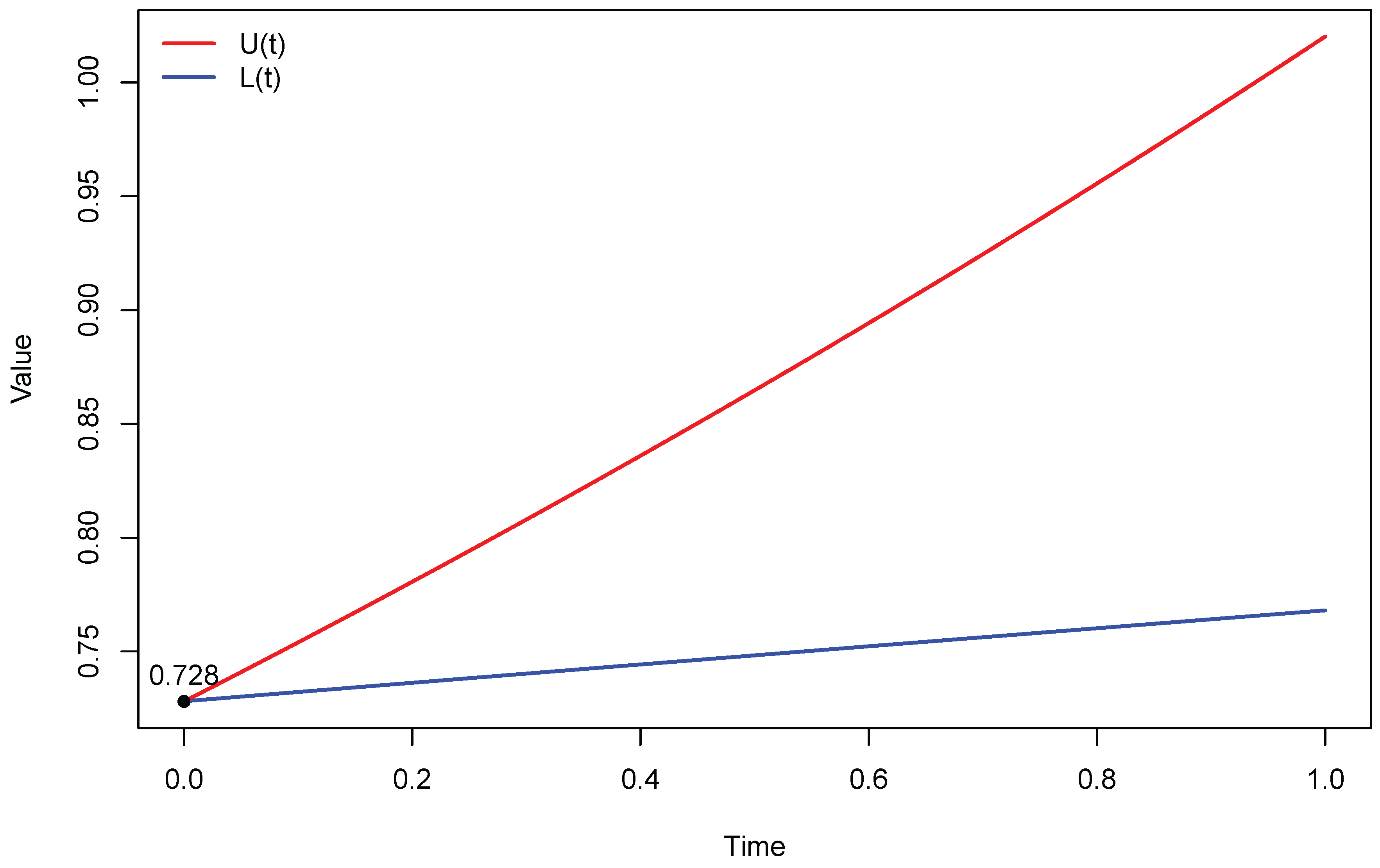
Figure 2.
Plots of U and L, for Row 2.
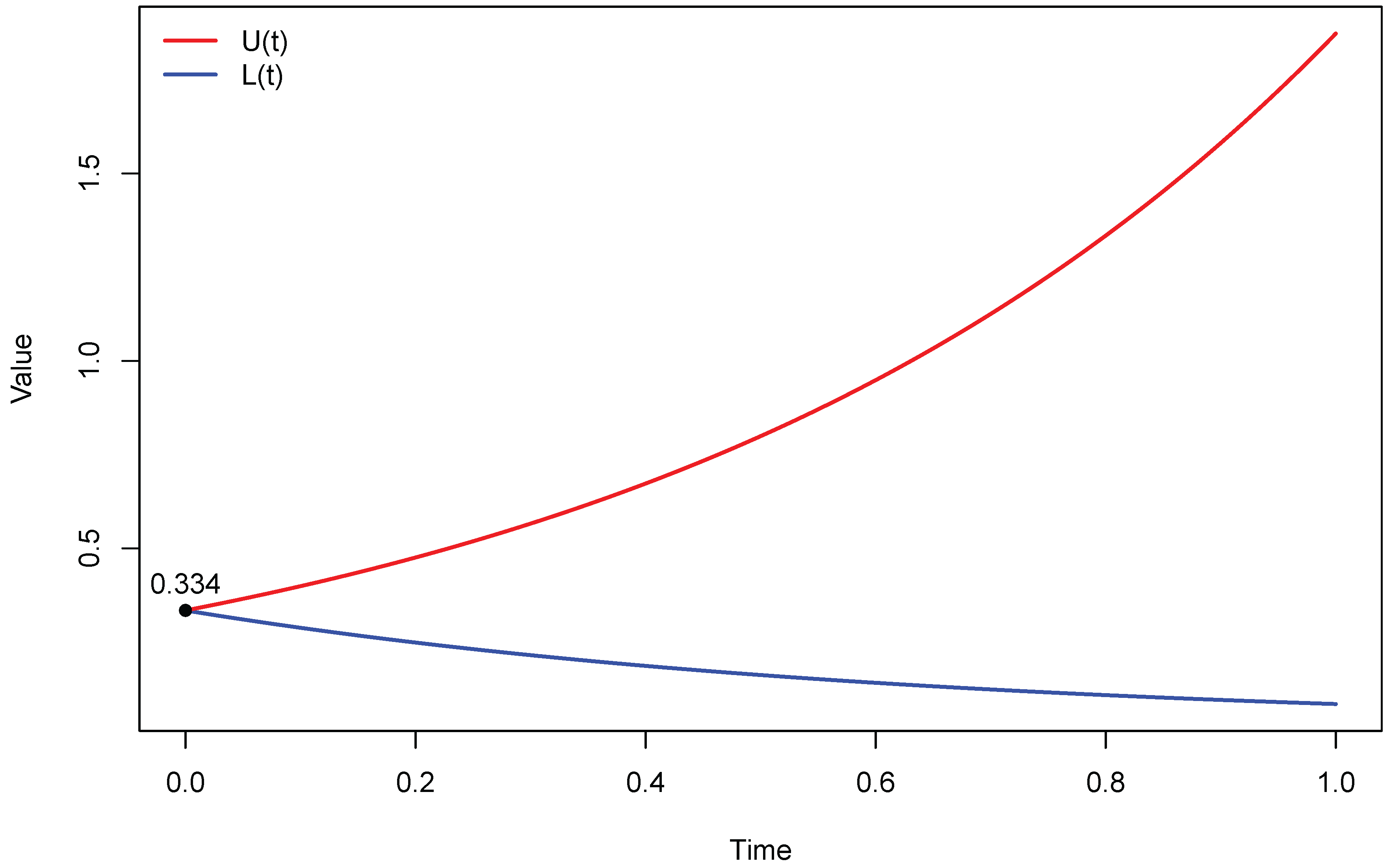
Figure 3.
Plots of U and L, for Row 3.
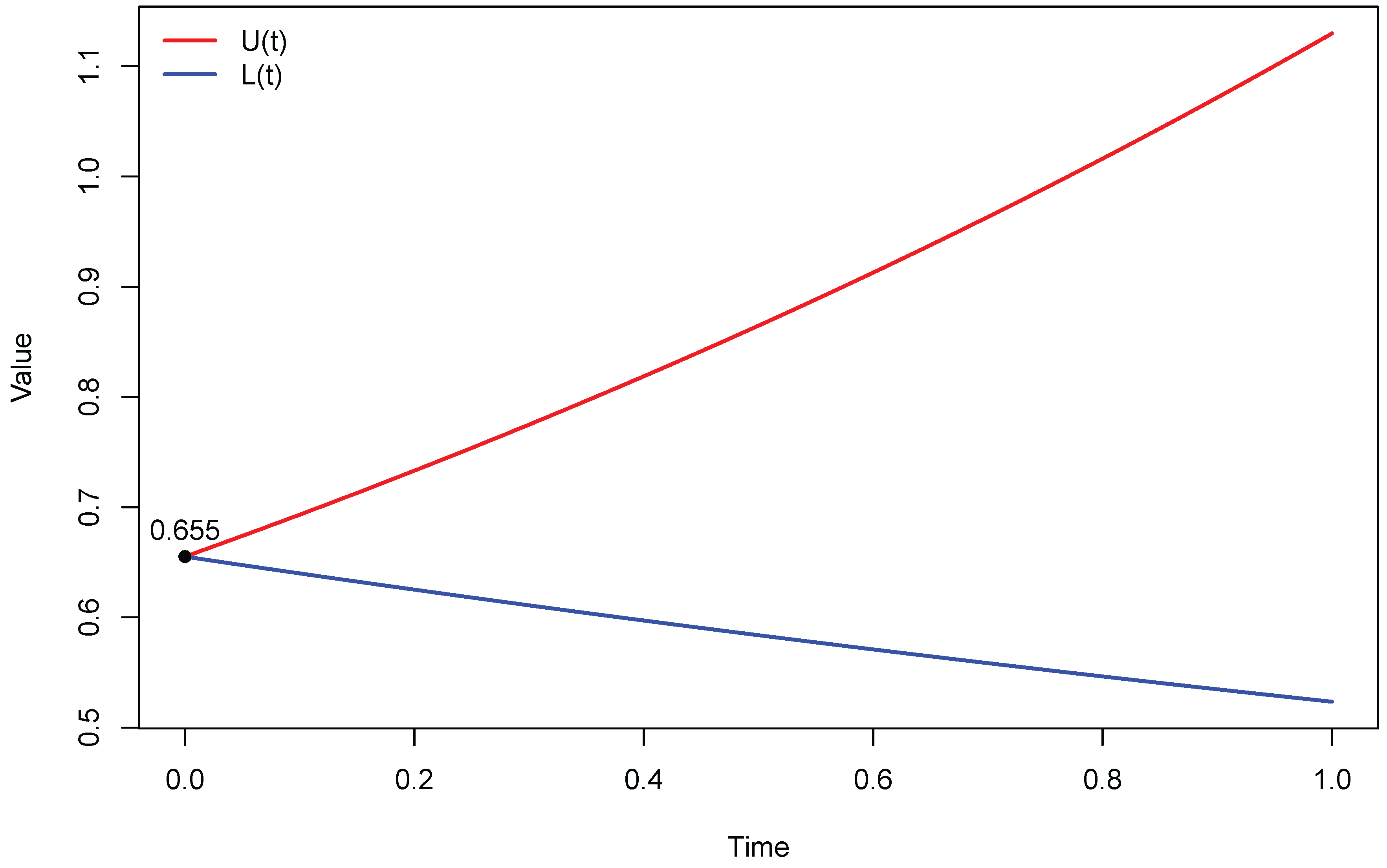
Figure 4.
Expectation and probability distribution for Row 1.
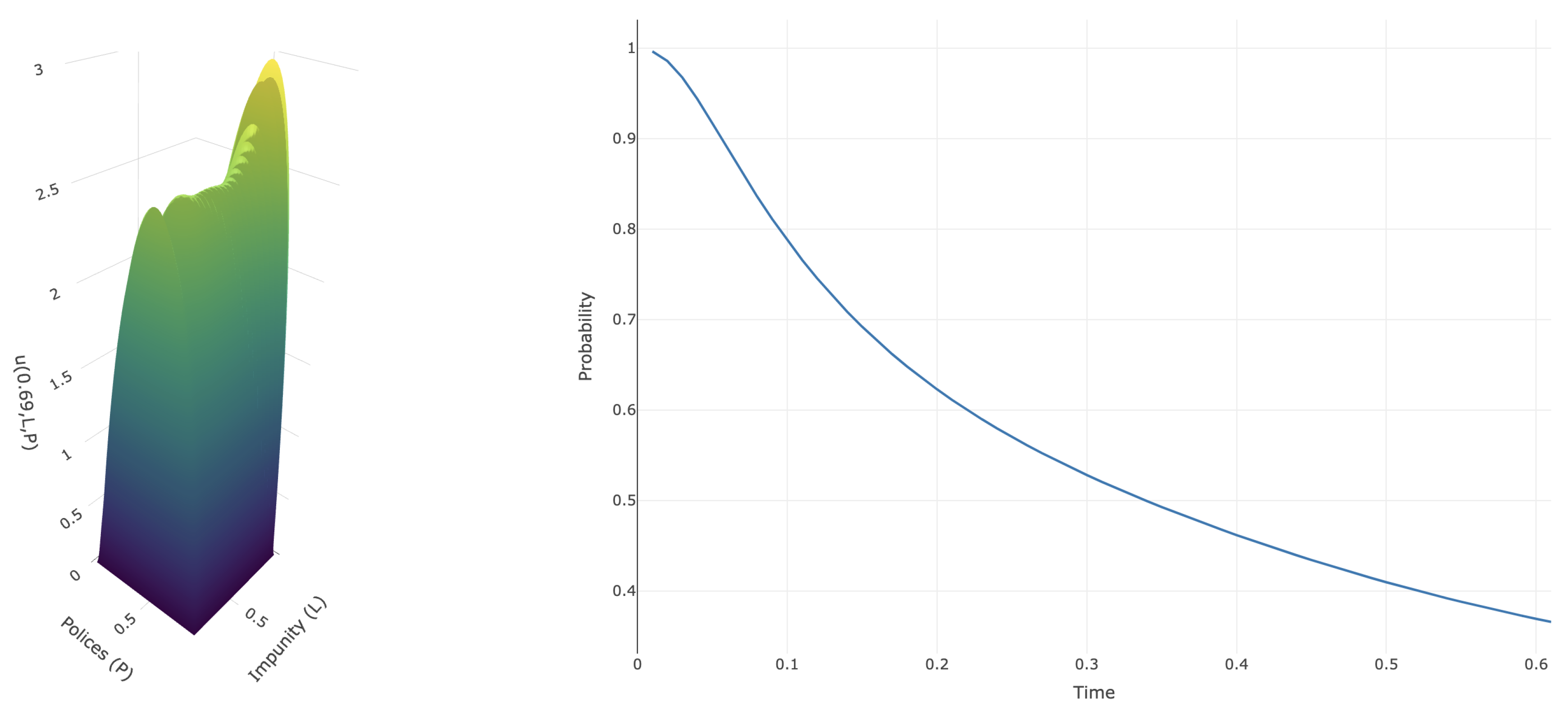
Figure 5.
Expectation and probability distribution for Row 2.
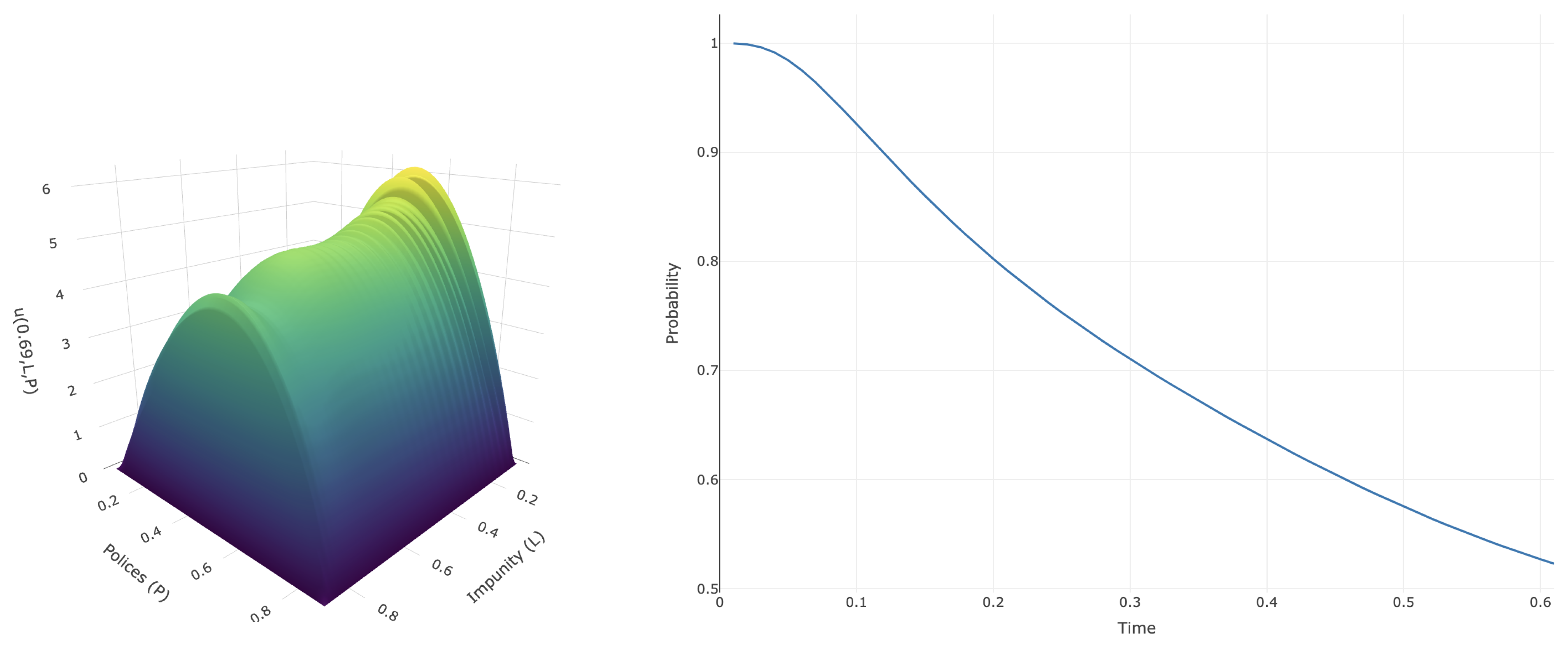
Figure 6.
Expectation and probability distribution for Row 3.
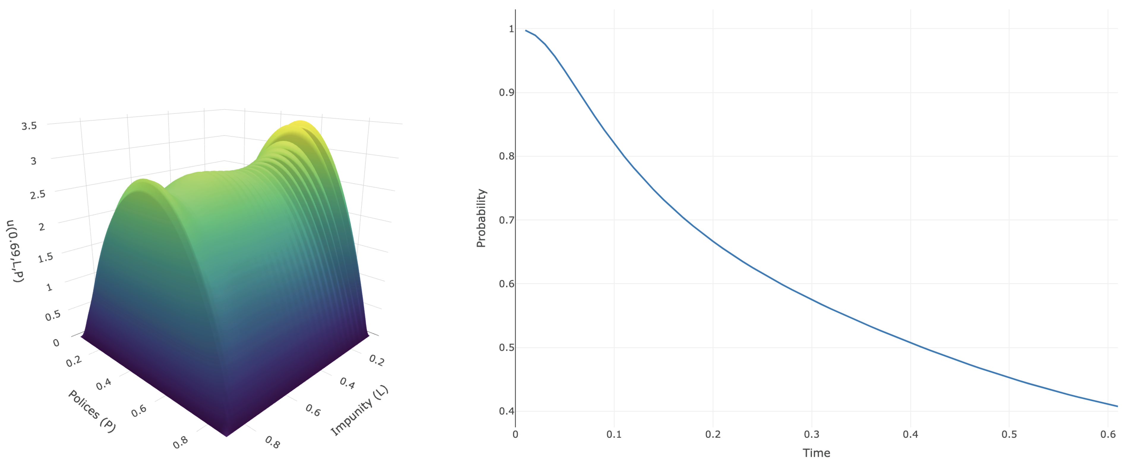

Table 1.
Corruption perception and impunity indices for Mexico.
| Year | 2015 | 2016 | 2017 | 2018 | 2019 | 2020 | 2021 | 2022 |
|---|---|---|---|---|---|---|---|---|
| 0.69 | 0.70 | 0.71 | 0.72 | 0.71 | 0.69 | 0.69 | 0.69 | |
| 0.2430 | 0.3258 | 0.3079 | 0.3016 | 0.4024 | 0.5033 | 0.4512 | 0.3992 |
Table 2.
Parameter values and corresponding equilibrium point , row by row.
| Row | ||||||||
|---|---|---|---|---|---|---|---|---|
| 1 | 0.7 | 0.005 | 0.1150 | 6.3705 | 0.1779 | 9.2310 | (0.6901, 0.0223, 0.0345) | 0.38275 |
| 2 | 0.7 | 0.025 | 0.1016 | 6.5525 | 0.1463 | 9.4913 | (0.6903, 0.1830, 0.2637) | 0.26811 |
| 3 | 0.4 | 0.005 | 0.0961 | 6.6186 | 0.1327 | 9.5857 | (0.6904, 0.0504, 0.0696) | 0.36520 |
| 4 | 0.4 | 0.025 | 0.0388 | 7.8422 | 0.0126 | 11.3586 | − |
Table 3.
Constants for the bounds L, U of , with .
| Row | |||||||
|---|---|---|---|---|---|---|---|
| 1 | 0.7280 | -0.0398 | 0.2563 | -1.0236 | 1.7517 | 1.0002 | 0.2722 |
| 2 | 0.3343 | -1.6007 | 1.6748 | 0.3128 | 0.0214 | 0.3548 | 0.0205 |
| 3 | 0.6551 | -0.3333 | 0.4704 | 0.4644 | 0.1907 | 0.7902 | 0.1351 |
Table 4.
Differences , for Row 1.
| Time | ||
|---|---|---|
| 0.1 | 0.732 | 0.022 |
| 0.2 | 0.736 | 0.044 |
| 0.3 | 0.740 | 0.068 |
| 0.4 | 0.744 | 0.092 |
| 0.5 | 0.748 | 0.117 |
| 0.6 | 0.752 | 0.143 |
| 0.7 | 0.756 | 0.169 |
| 0.8 | 0.760 | 0.196 |
| 0.9 | 0.764 | 0.224 |
| 1.0 | 0.768 | 0.252 |
Table 5.
Differences , for Row 2.
| Time | ||
|---|---|---|
| 0.1 | 0.287 | 0.112 |
| 0.2 | 0.248 | 0.228 |
| 0.3 | 0.214 | 0.353 |
| 0.4 | 0.184 | 0.491 |
| 0.5 | 0.161 | 0.641 |
| 0.6 | 0.140 | 0.813 |
| 0.7 | 0.122 | 1.010 |
| 0.8 | 0.107 | 1.236 |
| 0.9 | 0.094 | 1.499 |
| 1.0 | 0.084 | 1.789 |
Table 6.
Differences , for Row 3.
| Time | ||
|---|---|---|
| 0.1 | 0.639 | 0.054 |
| 0.2 | 0.625 | 0.108 |
| 0.3 | 0.610 | 0.165 |
| 0.4 | 0.596 | 0.223 |
| 0.5 | 0.583 | 0.282 |
| 0.6 | 0.570 | 0.344 |
| 0.7 | 0.558 | 0.407 |
| 0.8 | 0.545 | 0.476 |
| 0.9 | 0.534 | 0.540 |
| 1.0 | 0.523 | 0.606 |
Table 7.
Mean exit time and the point where u is maximal in .
| u | Row 1 | Row 2 | Row 3 |
|---|---|---|---|
| 1.0593 | 2.4617 | 1.3180 | |
| (0.1166, 0.5333, 2.9753) | (0.1166, 0.5166, 6.1320) | (0.1166, 0.5333, 3.4460) |
Table 8.
Values of for different rows and times t.
| Time | Row 1 | Row 2 | Row 3 |
|---|---|---|---|
| 0.05 | 0.917115 | 0.984423 | 0.934144 |
| 0.1 | 0.787826 | 0.925974 | 0.820086 |
| 0.2 | 0.622980 | 0.802421 | 0.666594 |
| 0.3 | 0.528259 | 0.710652 | 0.575021 |
| 0.4 | 0.461874 | 0.637164 | 0.507432 |
| 0.5 | 0.409736 | 0.575314 | 0.452671 |
| 0.6 | 0.369312 | 0.527094 | 0.411072 |
Table 9.
Values of for each domain and for the three parameter rows of Table 2.
Table 9.
Values of for each domain and for the three parameter rows of Table 2.
| Row i | ||
|---|---|---|
| Row 1 | 0.1437515 | |
| 0.1437535 | ||
| 0.5624885 | ||
| Row 2 | 0.2920392 | |
| 0.2924792 | ||
| 0.9923660 | ||
| Row 3 | 0.1578433 | |
| 0.1578498 | ||
| 0.6094088 |
Disclaimer/Publisher’s Note: The statements, opinions and data contained in all publications are solely those of the individual author(s) and contributor(s) and not of MDPI and/or the editor(s). MDPI and/or the editor(s) disclaim responsibility for any injury to people or property resulting from any ideas, methods, instructions or products referred to in the content. |
© 2025 by the authors. Licensee MDPI, Basel, Switzerland. This article is an open access article distributed under the terms and conditions of the Creative Commons Attribution (CC BY) license (http://creativecommons.org/licenses/by/4.0/).
Copyright: This open access article is published under a Creative Commons CC BY 4.0 license, which permit the free download, distribution, and reuse, provided that the author and preprint are cited in any reuse.


