An Axiomatic Theory of Quaternionic Probability Extending Kolmogorov’s Framework

1. Introduction

The foundations of modern probability theory were established by Kolmogorov [1], and subsequently developed in great detail in classical texts such as Billingsley [2], Doob [3], Feller [4], and Parthasarathy [5]. This framework, based on real-valued measures on sigma-algebras, has proven remarkably successful in describing a wide variety of stochastic phenomena. Nevertheless, over the past decades there has been increasing interest in extending the notion of probability beyond the real line, in order to model systems where interference, order-dependence, or non-commutativity play a fundamental role.

Already in the mid-20th century, Feynman speculated on the role of negative probabilities in quantum theory [6], while Khrennikov and others explored generalized frameworks for probability, including non-Kolmogorovian and ppp-adic formulations [7,8]. In parallel, noncommutative probability theory emerged in operator algebras, with Accardi [9], Accardi–Cecchini [10], Voiculescu [11], Speicher [12], Wysoczański [13], and Kümmerer [14] among the leading contributors. These works highlighted that probabilistic notions such as independence and conditional expectation admit multiple, non-equivalent generalizations once the commutativity of real-valued measures is abandoned.

Quaternions, introduced by Hamilton in the 19th century [15], have also played a fundamental role in mathematical physics. Quaternionic analysis [16], quaternionic quantum mechanics [17–19], and quaternionic differential operators [20] provided natural frameworks for describing rotations, spin, and field theories where complex numbers are not sufficient. More recently, Danielewski and Jadczyk [21] have revisited the foundations of quaternionic quantum mechanics, and Colombo, Sabadini, and Struppa [22] developed a functional calculus for slice hyperholomorphic functions, reinforcing the modern analytic foundations of quaternion-valued mathematics.

At the same time, practical applications of quaternionic probability and statistics have emerged in signal processing and image analysis. For instance, quaternionic Fourier transforms [25], principal component analysis [24], and augmented statistics of quaternion random variables [23] have shown how quaternion-valued frameworks can capture multi-dimensional correlations in ways that real or complex approaches cannot. Recent mathematical work, such as Wang and Zhang’s quaternionic Mahler measure [26], further illustrates that the study of measures with values in $\mathbb{H}$ is both mathematically natural and actively developing.

Despite these advances, a systematic axiomatic theory of quaternionic probability—comparable in rigor to Kolmogorov’s framework, but extending it into the noncommutative domain of quaternions—has not yet been established. The goal of this work is to provide such a theory: to define quaternionic probability spaces, state coherent axioms, and develop the corresponding notions of conditional probability, independence, random variables, processes, and information measures. By doing so, we show how classical probability [1–5] and quantum complex probability [6,7,9] appear as special cases, while new phenomena—such as order-dependent conditional probabilities, noncommutative independence, and quaternionic transport equations—arise uniquely in the quaternionic setting.

This paper is structured as follows. In Section 2 we introduce the axioms of quaternionic probability and establish their basic consequences. Sections 3 and 4 develop conditional probabilities, Bayes’ rules, and notions of independence in the noncommutative context. In Sections 5 and 6 we define quaternionic random variables, expectations, and observables. Sections 7 and 8 extend the theory to stochastic processes and derive quaternionic continuity and Fokker–Planck-type equations. Section 9 studies quaternionic Markov chains, while Section 10 develops a framework for quaternionic information theory. In Section 11 we compare the quaternionic framework to classical and complex probability, and in Section 12 we present illustrative examples and potential applications. Technical details are collected in Section 16.

To the best of our knowledge, no complete axiomatization of probability over the quaternionic algebra has been established in the literature. Previous works have considered noncommutative probability in the context of operator algebras or complex Hilbert spaces, but a direct extension of Kolmogorov’s axioms to quaternions has not been systematically developed. The present work aims to fill this gap by constructing a rigorous quaternionic probability theory and by illustrating its distinctive features through both mathematical results and concrete examples.

2. Quaternionic Probability Spaces and Axioms

We begin by extending Kolmogorov’s axioms [1] to quaternion-valued measures. Throughout, let $\mathbb{H}$ denote the skew field of quaternions, with scalar part $Sc\left(q\right)$ and vector part $Vec\left(q\right)$.The set of unit quaternions is denoted by ${\mathbb{S}}^3=\{q\in \mathbb{H}:\left|q\right|=1\}.$

Definition 2.1

(Quaternionic probability space).

A quaternionic probability space is a triple

$$(\mathsf{\Omega },\mathcal{F},{\mathbb{P}}_{\mathbb{H}}),$$

where:

• $\mathsf{\Omega }$ a sample space,
• $\mathcal{F}$ is a $\sigma$ -algebra of subsets of $\mathsf{\Omega }$,
• ${\mathbb{P}}_{\mathbb{H}}: \mathcal{F}\to \mathbb{H}$ is a set function satisfying the axioms below.

Axiom 2.1 (Normalization).

$$Sc{\mathbb{P}}_{\mathbb{H}}\left(\mathsf{\Omega }\right)=1.$$

Axiom 2.2 (Quaternionic $\mathit{\sigma }$  -additivity).

  

For any countable collection of pairwise disjoint sets $E_1,E_2,\dots \in \mathcal{F}$,

$${\mathbb{P}}_{\mathbb{H}}\left(\bigcup _{n=1}^{\infty }{E}_n\right)=\sum _{n=1}^{\infty }{\mathbb{P}}_{\mathbb{H}}\left(E_n\right),$$

where convergence is taken in the quaternionic norm.

Axiom 2.3 (Scalar positivity).

$$Sc{\mathbb{ }\mathbb{P}}_{\mathbb{H}}\left(E\right)\ge 0 \mathrm{for} \mathrm{all} E\in \mathcal{F}.$$

Axiom 2.4 (Complement).

$${\mathbb{ }\mathbb{P}}_{\mathbb{H}}\left(E^C\right)=1-{\mathbb{ }\mathbb{P}}_{\mathbb{H}}\left(E\right).$$

Axiom 2.5 (Boundedness).

$$\left|{\mathbb{ }\mathbb{P}}_{\mathbb{H}}\left(E\right)\right|\le 1 \mathrm{for} \mathrm{all} E\in \mathcal{F}.$$

Lemma 2.1 (Classical reduction).

  

The scalar part

$$P\left(E\right)≔Sc{\mathbb{ }\mathbb{P}}_{\mathbb{H}}\left(E\right).$$

defines a classical probability measure on ($\mathsf{\Omega },\mathcal{F})$.

Proof. 

Immediate from Axioms 2.1–2.3.

Proposition 2.1 (Modulus–phase factorization).

  

Every quaternionic probability can be uniquely written as

$${\mathbb{ }\mathbb{P}}_{\mathbb{H}}\left(E\right)=P\left(E\right)U\left(E\right),$$

where $\mathbb{P}\left(E\right)\in \left[\mathrm{0,1}\right]$ is the classical probability of $E$ and $U\left(E\right)\in S^3$ is a unit quaternion.

Interpretation. The scalar component $\mathbb{P}\left(E\right)$ captures the usual frequency interpretation, while the unit quaternion $U\left(E\right)$ encodes an additional “phase” or orientation, absent in the classical case.

This axiomatic structure establishes quaternionic probability as a genuine extension of Kolmogorov’s framework. In the next section we explore the consequences for conditional probabilities and Bayes’ rule in a noncommutative setting.

3. Conditional Probabilities and Bayes’ Theorem.

One of the main novelties of quaternionic probability is that conditionalization becomes inherently noncommutative. Because quaternionic multiplication does not commute, we must distinguish between right and left conditional probabilities.

Definition 3.1 (Right conditional probability).

  

For events $A,B\in \mathcal{F}$ with ${\mathbb{ }\mathbb{P}}_{\mathbb{H}}\left(B\right)\ne 0$, the right conditional probability of $A$ given $B$ is defined by

$${\mathbb{P}}^R\left(A|B\right)≔{\mathbb{ }\mathbb{P}}_{\mathbb{H}}\left(A\bigcap B\right) {\left({\mathbb{ }\mathbb{P}}_{\mathbb{H}}\left(B\right)\right)}^{-1}.$$

Definition 3.2 (Left conditional probability).

  

For events $A,B\in \mathcal{F}$ with ${\mathbb{ }\mathbb{P}}_{\mathbb{H}}\left(B\right)\ne 0$, the left conditional probability of $A$ given $B$ is defined by

$${\mathbb{P}}^L\left(A|B\right)≔ {\left({\mathbb{ }\mathbb{P}}_{\mathbb{H}}\left(B\right)\right)}^{-1}{\mathbb{ }\mathbb{P}}_{\mathbb{H}}\left(A\bigcap B\right).$$

Proposition 3.1 (Scalar reduction).

  

For both left and right conditionals,

$$Sc {\mathbb{P}}^R\left(A|B\right)=Sc {\mathbb{P}}^L\left(A|B\right)=P\left(A|B\right).$$

where P $P\left(A|B\right)$ is the classical conditional probability.

Proof. 

Since scalar parts commute, the difference between left and right multiplications disappears when taking $Sc\left(\cdot \right) .$

Proposition 3.2 (Order-dependence).

In general,

$${\mathbb{P}}^R\left(A|B\right)\ne {\mathbb{P}}^L\left(A|B\right).$$

Thus, conditional probabilities encode not only relative frequency but also the order of information update.

Theorem 3.1 (Right Bayes’ rule).

  

Let $\left\{B_j\right\}$ be a finite or countable partition of $\mathsf{\Omega }$ with ${\mathbb{ }\mathbb{P}}_{\mathbb{H}}\left(B_j\right)\ne 0$. Then, for any $A\in \mathcal{F}$,

$${\mathbb{P}}^R\left(B_k|A\right)={\displaystyle \frac{{\mathbb{P}}^R\left(A|B_k\right){\mathbb{ }\mathbb{P}}_{\mathbb{H}}\left(B_k\right)}{\sum _j{\mathbb{P}}^R\left(A|B_j\right){\mathbb{ }\mathbb{P}}_{\mathbb{H}}\left(B_j\right)}}.$$

Theorem 3.2 (Left Bayes’ rule).

  

Under the same assumptions,

$${\mathbb{P}}^L\left(B_k|A\right)={\left(\sum _j{\mathbb{P}}^R\left(A|B_j\right){\mathbb{ }\mathbb{P}}_{\mathbb{H}}\left(B_j\right)\right)}^{-1}{\mathbb{P}}^R\left(A|B_k\right){\mathbb{ }\mathbb{P}}_{\mathbb{H}}\left(B_k\right).$$

Remark 3.1.

• Both Bayes’ rules reduce to the classical one when all quaternionic phases commute.
• The distinction between left and right formulations reflects the noncommutative geometry of the quaternionic unit sphere ${\mathbb{S}}^3$.
• This framework naturally accommodates order-sensitive inference, where updating on $A$ then $B$ is not equivalent to updating on $B$ then $A$.

This section demonstrates that conditionalization in quaternionic probability is fundamentally noncommutative, giving rise to two inequivalent but consistent Bayes’ rules. In the next section we will investigate how these asymmetries manifest in different notions of independence.

4. Independence and Correlations.

In the quaternionic framework, the noncommutativity of multiplication implies that the notion of independence is no longer unique. We distinguish several types of independence and define quaternionic correlation.

Definition 4.1 (Strong independence).

  

Two events $A,B\in \mathcal{F}$ are said to be strongly independent if

$${\mathbb{ }\mathbb{P}}_{\mathbb{H}}\left(A\bigcap B\right)={\mathbb{ }\mathbb{P}}_{\mathbb{H}}\left(A\right){\mathbb{ }\mathbb{P}}_{\mathbb{H}}\left(B\right).$$

Definition 4.2 (Right independence).

  

Events $A,B$ are right independent if

$${\mathbb{ }\mathbb{P}}_{\mathbb{H}}\left(A\bigcap B\right)={\mathbb{P}}^R\left(A|B\right){\mathbb{ }\mathbb{P}}_{\mathbb{H}}\left(B\right).$$

Definition 4.3 (Left independence).

  

Events $A,B$ are left independent if

$${\mathbb{ }\mathbb{P}}_{\mathbb{H}}\left(A\bigcap B\right)={\mathbb{P}}_{\mathbb{H}}\left(B\right){\mathbb{P}}^L\left(A|B\right).$$

Definition 4.4 (Scalar independence).

  

Events $A,B$ are scalar independent if

$$P\left(A\bigcap B\right)=P\left(A\right)P\left(B\right),$$

where $P=Sc{\mathbb{ }\mathbb{P}}_{\mathbb{H}}$ is the underlying classical probability.

Proposition 4.1.

  

Strong independence  $⟹$   right independence, left independence, and scalar independence. The converses do not hold in general.

Proof. 

Strong independence directly implies equality under both left and right conditional definitions and yields the scalar condition. However, the reverse implications fail when quaternionic phases do not commute.

Definition 4.5 (Quaternionic correlation).

  

The quaternionic correlation between two events $A,B$ is defined as

$${ C}_{\mathbb{H}}\left(A,B\right){≔\mathbb{ }\mathbb{P}}_{\mathbb{H}}\left(A\bigcap B\right)-{\mathbb{ }\mathbb{P}}_{\mathbb{H}}\left(A\right){\mathbb{ }\mathbb{P}}_{\mathbb{H}}\left(B\right).$$

Proposition 4.2 (Scalar reduction of correlation).

  

The scalar part of quaternionic correlation is the classical covariance:

$${Sc C}_{\mathbb{H}}\left(A,B\right)≔P\left(A\bigcap B\right)-P\left(A\right)P\left(B\right).$$

Remark 4.1.

• In the classical case, independence is unique; here, different forms of independence reflect the underlying noncommutative structure.
• The quaternionic correlation captures deviations not only in scalar probability but also in vectorial phase coherence.
• Order effects (left vs. right independence) provide a natural mathematical description of phenomena where the sequence of conditioning matters.

This section shows that the richness of quaternionic probability emerges already at the level of independence. Multiple notions coexist, and correlations now carry both scalar and vectorial information. In the next section we will introduce quaternionic random variables and define expectations and moments.

5. Quaternionic Random Variables and Expectation.

Having defined quaternionic probability measures, we now extend the framework to random variables, expectations, and moments. The key novelty is that expectations become quaternion-valued, and inequalities must be interpreted via their scalar components.

Definition 5.1 (Quaternionic random variable).

  

A quaternionic random variable is a measurable map

$$\mathrm{X}:\mathsf{\Omega }\to \mathbb{H}.$$

The distribution of $X$ is the quaternionic measure

$${\mu }_X\left(B\right) :={\mathbb{ }\mathbb{P}}_{\mathbb{H}}\left(X^{-1}\left(B\right)\right), B\subseteq \mathbb{H}.$$

Definition 5.2 (Expectation).

  

The expectation of $X$ is defined by

$${\mathbb{E}}_{\mathbb{H}}\left[X\right]={\int }_{\mathsf{\Omega }}X\left(\omega \right)d{\mathbb{P}}_{\mathbb{H}}\left(\omega \right).$$

When ${\mathbb{P}}_{\mathbb{H}}$​ is expressed in modulus–phase form ${\mathbb{P}}_{\mathbb{H}}=PU$, this integral can be interpreted as

$${\mathbb{E}}_{\mathbb{H}}\left[X\right]={\int }_{\mathsf{\Omega }}X\left(\omega \right)U\left(\omega \right)dP\left(\omega \right)$$

with $P$ the scalar probability and $U\left(\omega \right)\in {\mathbb{S}}^3$ a local quaternionic phase.

Proposition 5.1 (Scalar expectation).

  

The scalar part of the quaternionic expectation is the classical expectation:

$${Sc \mathbb{E}}_{\mathbb{H}}\left[X\right]=\mathbb{E}\left[X\right],$$

where $\mathbb{E}\left[X\right]$ is the usual expectation with respect to $P=Sc{\mathbb{ }\mathbb{P}}_{\mathbb{H}}$.

Definition 5.3 (Variance).

  

The variance of $X$ is defined as

$${Var}_{\mathbb{H}}\left(X\right):={\mathbb{ }\mathbb{E}}_{\mathbb{H}}\left[{\left|X\right|}^2\right]-{\left|{\mathbb{E}}_{\mathbb{H}}\left[X\right]\right|}^2$$

Proposition 5.2 (Scalar variance).

  

The scalar part of the quaternionic variance coincides with the classical variance:

$$Sc {Var}_{\mathbb{H}}\left(X\right)=Var\left(X\right).$$

Theorem 5.1 (Markov inequality, quaternionic form).

  

Let $X\ge 0$ be a real-valued random variable on a quaternionic probability space. Then, for any $\alpha >0$,

$$P\left(X\ge \alpha \right)\le {\displaystyle \frac{\mathbb{E}\left[X\right]}{\alpha }}$$

where $P=Sc{\mathbb{ }\mathbb{P}}_{\mathbb{H}}$.

Remark. 

The inequality remains scalar because order in $\mathbb{H}$ is not defined; only the real measure governs tail bounds.

Theorem 5.2 (Chebyshev inequality, quaternionic form).

  

For any real-valued $X$ with finite variance,

$$P\left(\left|X-\mathbb{E}\left[X\right]\right|\ge \epsilon \right)\le {\displaystyle \frac{\mathbb{E}\left[X\right]}{{\epsilon }^2}}$$

Again, the scalar distribution $P$ controls concentration, while the quaternionic components contribute through higher-order coherence rather than tail probabilities.

Remark 5.1.

  

• Expectations and variances carry quaternionic information, but inequalities remain scalar because order is defined only in $\mathbb{R}$.
• The vector components of $\mathbb{E}\left[X\right]$ may encode directional or phase-like features of the distribution.

This section establishes the basic theory of quaternionic random variables. In the next section we introduce projections onto complex subalgebras and observables, showing how real measurements can be extracted from quaternionic distributions.

6. Transformations, Projections, and Observables.

While quaternionic random variables may take values in the full noncommutative algebra $\mathbb{H}$, in practice one often measures or analyzes their behavior through projections onto real or complex subalgebras. This section formalizes such transformations and introduces the notion of observables.

Definition 6.1 (Projection onto a subalgebra).

  

For a fixed imaginary unit $u\in \{i,j,k$}, define the projection

$${\pi }_u:\mathbb{H}\to {\mathbb{C}}_u≔\left\{a+bu:a,b\in \mathbb{R}\right\}$$

by

$${\pi }_u\left(a+bi+cj+dk\right)=a+bu.$$

Proposition 6.1.

  

For any quaternionic random variable $X$, the projection $X^{\left(u\right)}≔{\pi }_u\left(X\right)$ is a complex-valued random variable with respect to the underlying scalar probability measure $P=Sc{\mathbb{ }\mathbb{P}}_{\mathbb{H}}$.​

Definition 6.2 (Observable).

  

Let $\mathrm{X}:\mathsf{\Omega }\to \mathbb{H}$ be a quaternionic random variable and $u\in \{i,j,k\}$. The observable associated with direction uuu is defined as

$$O_u\left(X\right):=Sc(X u^{*}).$$

This extracts a real-valued random variable aligned with the chosen imaginary axis.

Proposition 6.2 (Expectation of observables).

  

For each uuu, the expectation of the observable satisfies

$$\mathbb{E}\left[O_u\left(X\right)\right]={Sc \mathbb{E}}_{\mathbb{H}}\left[X u^{*}\right].$$

Theorem 6.1  (Reduction to classical/complex cases).

• If $\mathrm{U}\left(\mathrm{E}\right)\equiv 1$ for all $\mathrm{E}$, then quaternionic probability reduces to classical probability.
• If all phases $\mathrm{U}\left(\mathrm{E}\right)$ lie within a single complex subalgebra ${\mathbb{C}}_{\mathrm{u}}\subset \mathbb{H}$, then quaternionic probability reduces to complex probability, structurally equivalent to standard quantum mechanics.

Remark 6.1.

• Projections and observables provide the link between quaternionic models and experimentally accessible quantities.
• This mirrors the role of self-adjoint operators in quantum mechanics, but extended to the richer quaternionic setting.

This section clarifies how quaternionic random variables can be connected to measurable outputs. In the next section we will extend the framework to stochastic processes and derive quaternionic versions of balance and continuity equations.

7. Quaternionic Processes and Continuity Equations.

In classical probability, stochastic processes are families of random variables indexed by time, whose evolution is described by balance or continuity equations. In the quaternionic setting, these structures generalize to quaternion-valued densities and currents.

Definition 7.1 (Quaternionic stochastic process).

  

A quaternionic stochastic process is a family of quaternionic random variables

$${\{X_{t}t:\Omega \to \mathbb{H}\}}_{t\ge 0}\mathit{},$$

adapted to some filtration ${{\{\mathcal{F}}_t\}}_{t\ge 0}$.

Definition 7.2 (Quaternionic probability density).

  

A quaternionic-valued density is a function

$$\rho \left(x,t\right)={\rho }_0\left(x,t\right)+{\rho }_1\left(x,t\right)i+{\rho }_2\left(x,t\right)j+{\rho }_3(x,t)k$$

with ${\rho }_{\mathcal{l}}\left(x,t\right)\in \mathbb{R}$. Its scalar part ${\rho }_0$​ represents the classical probability density.

Definition 7.3 (Quaternionic current).

  

The probability current is a quaternionic vector field

$$J\left(x,t\right)=J_0\left(x,t\right)+J_1\left(x,t\right)i+J_2\left(x,t\right)j+J_3(x,t)k$$

with $J_m\left(x,t\right)\in {\mathbb{R}}^d$.

Theorem 7.1 (Quaternionic continuity equation).

  

For any region $V\subset {\mathbb{R}}^d$,

$${\displaystyle \frac{d}{dt}}{\int }_V\rho \left(x,t\right)dx=-{\int }_{\partial V}J\left(x,t\right)\cdot n dS+{\int }_{V}S\left(x,t\right)dx,$$

where $S\left(x,t\right)$ is a quaternionic source term.

In differential form,

$${\partial }_t\rho \left(x,t\right)+\nabla \cdot J\left(x,t\right)=S\left(x,t\right).$$

Proof. 

Follows from quaternionic integration and the divergence theorem applied componentwise.

Proposition 7.1 (Scalar reduction).

  

The scalar part of the continuity equation is

$${\partial }_t{\rho }_0\left(x,t\right)+\nabla \cdot J_0\left(x,t\right)=S_0\left(x,t\right).$$

which is the classical continuity equation.

Remark 7.1.

• The scalar component governs ordinary conservation of probability.
• The vectorial components describe additional degrees of freedom, such as orientation or phase transport in quaternionic space.
• This structure allows for richer dynamics while ensuring that the real part remains a valid probability density.

This section establishes the quaternionic continuity equation as the fundamental balance law of quaternionic probability. In the next section we derive transport equations and diffusion dynamics, including a quaternionic Fokker–Planck equation.

8. Transport and the One-Dimensional Case.

The quaternionic continuity equation provides the general balance law for probability densities. In this section, we introduce specific transport models and study their one-dimensional reduction.

Definition 8.1 (Quaternionic drift–diffusion current).

  

Given a velocity field $v\in {\mathbb{H}}^d$and diffusion coefficient $D>0$, the quaternionic probability current is modeled as

$$J\left(x,t\right)=v \rho \left(x,t\right)-D\nabla \rho \left(x,t\right).$$

Theorem 8.1 (Quaternionic Fokker–Planck equation).

  

Substituting the drift–diffusion current into the continuity equation yields

$${\partial }_t\rho \left(x,t\right)=-\left(v\cdot \nabla \right)\rho \left(x,t\right)+D{\nabla }^2\rho \left(x,t\right).$$

Proof. 

Direct substitution and application of the divergence theorem.

Proposition 8.1 (Component form).

Writing $\rho ={\rho }_0+{\rho }_{1}i+{\rho }_{2}j+{\rho }_{3}k$, each component satisfies

$${\partial }_t{\rho }_m\left(x,t\right)=-\left(v\cdot \nabla \right){\rho }_m\left(x,t\right)+D{\nabla }^2{\rho }_m\left(x,t\right), m=\mathrm{0,1},\mathrm{2,3}.$$

Corollary 8.1 (Scalar reduction).

  

The scalar part ${\rho }_0$​ evolves according to the classical Fokker–Planck equation, while the vector parts ${\rho }_1,{\rho }_2,{\rho }_3$​ evolve as coupled drift–diffusion fields without affecting normalization.

Definition 8.2 (One-dimensional transport).

  

In one dimension,

$${\partial }_t{\rho }_m\left(x,t\right)=-{\partial }_x\left({v\rho }_x\left(x,t\right)\right)+D{\partial }_x^2{\rho }_x\left(x,t\right).$$

Proposition 8.2 (Solution structure in 1D).

  

For constant $v$ and $D$, the solution takes the form

$$\rho \left(x,t\right)={\displaystyle \frac{1}{\sqrt{4\pi Dt}}}\exp \left(-{\displaystyle \frac{{\left(x-vt\right)}^2}{4Dt}}\right)U,$$

where $U\in {\mathbb{S}}^3$ is a unit quaternion encoding the initial phase orientation.

Remark 8.1.

• The one-dimensional case illustrates how quaternionic probability preserves the scalar Gaussian kernel while enriching it with quaternionic phase structure.
• The evolution of vectorial components can be interpreted as rotational diffusion in quaternionic space.

This section demonstrates how transport and diffusion extend naturally into the quaternionic setting, reducing to classical equations in the scalar component but enriching the dynamics with quaternionic phases. In the next section, we introduce quaternionic Markov chains and their generators.

9. Quaternionic Markov Chains and Generators

Markov processes describe systems evolving by local transitions between states. In the quaternionic setting, transition probabilities are replaced by quaternionic-valued entries, introducing order-dependence and noncommutativity.

Definition 9.1 (Quaternionic stochastic matrix).

  

A matrix $P=\left(p_{ij}\right)\in M_n(\mathbb{H}$) is a quaternionic stochastic matrix if:

• $p_{ij}\in \mathbb{H},$
• $Sc\left(p_{ij}\right)\ge 0$for all$i,j,$
• $\sum _{j}Sc\left(p_{ij}\right)=1$for each row $i,$
• $\left|p_{ij}\right|\le 1.$

Definition 9.2 (Quaternionic Markov chain).

  

A process ${\left\{X_t\right\}}_{t\ge 0}$​ with state space $\left\{1,\dots ,n\right\}$ is a quaternionic Markov chain if

$${\mathbb{P}}_{\mathbb{H}}\left(X_{t+1}=j \right| X_t=i, history )=p_{ij},$$

with $\left(p_{ij}\right)$ a quaternionic stochastic matrix.

Proposition 9.1 (Evolution of distributions).

  

If ${\pi }^{\left(0\right)}\in {\mathbb{H}}^n$ is the initial distribution, then

$${\pi }^{(t+1)}={\pi }^{\left(t\right)}P$$

Lemma 9.1 (Scalar reduction).

  

The scalar part of ${\pi }^{\left(t\right)}$ evolves as a classical Markov chain with transition matrix $Sc\left(P\right).$

Definition 9.3 (Quaternionic generator).

  

In continuous time, a quaternionic generator is a matrix $Q=\left(q_{ij}\right)\in M_n\left(\mathbb{H}\right)$ satisfying:

5.

$Sc\left(q_{ij}\right)\ge 0$for $i\ne j$.

6.

$\sum _{j}Sc\left(q_{ij}\right)=0$for each row $i.$

The evolution is given by

$$\pi \left(t\right)=\pi \left(0\right)e^{Qt}$$

Theorem 9.1 (Semigroup property).

  

The family $T\left(t\right)=e^{Qt}$ forms a semigroup preserving scalar normalization:

$$\sum _{i}Sc\left({\pi }_i\left(t\right)\right)=1\mathrm{for} \mathrm{all} \mathrm{t}\ge 0.$$

Definition 9.4 (Stationary distribution).

  

A vector $\pi \in H^n$ is stationary if

$$\pi P=\pi \left(discrete time\right), \pi Q=0 \left(continuous time\right).$$

Theorem 9.2 (Scalar stationarity).

  

If $\pi$ is stationary in the quaternionic sense, then $Sc\left(\pi \right)$ is a stationary distribution for the associated classical Markov chain.

Remark 9.1.

• The scalar structure ensures consistency with classical Markov theory.
• Vectorial components enrich the model by introducing noncommutative order effects and quaternionic phase rotations.
• Applications include systems where both transition frequencies and phase-like correlations are relevant.

This section establishes quaternionic Markov processes, extending the classical theory with quaternion-valued transition structures. In the next section, we build on this framework to define entropy, divergence, and information measures in quaternionic probability.

10. Quaternionic Information Theory

Information theory provides a quantitative framework to study uncertainty, divergence, and coherence in probability distributions. Extending these notions to quaternionic probability requires separating scalar uncertainty from vectorial coherence.

Definition 10.1 (Scalar entropy).

  

For a quaternionic density $\rho \left(x\right)$, the scalar entropy is defined as

$$H\left({\rho }_0\right)=-\int {\rho }_0\left(x\right)\log {\rho }_0\left(x\right)dx,$$

where ${\rho }_0=Sc\left(\rho \right)$.

This coincides with the classical Shannon entropy.

Definition 10.2 (Vector coherence functional).

  

The vectorial coherence of $\rho$ is defined as

$$I_{vec}\left(\rho \right)=\int ‖Vec\left(\rho \left(x\right)\right)‖dx.$$

• $I_{vec}=0$: purely classical distribution.
• $I_{vec}>0$: quaternionic coherence beyond real probability.

Definition 10.3 (Quaternionic entropy).

  

The quaternionic entropy is defined by

$$H_{\mathbb{H}}\left(\rho \right)=H\left({\rho }_0\right)+\lambda I_{vec}\left(\rho \right)$$

where $\lambda >0$ is a weighting parameter.

Definition 10.4 (Quaternionic divergence).

  

For two densities $\rho$,$\sigma$, define

$$D_{\mathbb{H}}\left(\rho \parallel \sigma \right)=\int [{\rho }_0\left(x\right)\log {\displaystyle \frac{{\rho }_0\left(x\right)}{{\sigma }_0\left(x\right)}}+{‖Vec\left(\rho \left(x\right)\right)-Vec\left(\sigma \left(x\right)\right)‖}^2]dx.$$

• The first term is the classical Kullback–Leibler divergence.
• The second measures the mismatch of quaternionic vector phases.

Theorem 10.1 (Non-negativity).

$$D_{\mathbb{H}}\left(\rho \parallel \sigma \right)\ge 0, and D_{\mathbb{H}}\left(\rho \parallel \sigma \right)\iff \rho =\sigma$$

Theorem 10.2 (Monotonicity under channels).

  

If $\mathsf{\Phi }$ is a linear map preserving scalar normalization, then

$$D_{\mathbb{H}}\left(\mathsf{\Phi }\left(\rho \right)\parallel \mathsf{\Phi }\left(\sigma \right)\right)\le D_{\mathbb{H}}\left(\rho \parallel \sigma \right)$$

This extends the classical data-processing inequality.

Remark 10.1.

• The scalar entropy reflects classical uncertainty.
• The coherence functional captures quaternionic information not visible in real probabilities.
• Divergence in quaternionic probability simultaneously measures probabilistic and orientational mismatch.

This section introduces entropy, coherence, and divergence in quaternionic probability, laying the foundation for a broader information-theoretic framework. In the next section, we compare the quaternionic model with its classical and complex counterparts.

11. Comparison with Classical and Complex Cases.

The quaternionic framework simultaneously generalizes both classical Kolmogorov probability and complex quantum probability. This section highlights how these theories are embedded as special cases.

Proposition 11.1 (Classical reduction).

  

If all quaternionic phases are trivial, $U\left(E\right)\equiv 1$, then

$${\mathbb{P}}_{\mathbb{H}}\left(\mathrm{E}\right)=\mathbb{P}\left(E\right)\in \left[\mathrm{0,1}\right]\subset \mathbb{R}.$$

• Left and right conditional probabilities coincide.
• Independence reduces to the classical definition.
• The continuity and transport equations reduce to their classical forms.

Thus, classical probability [1,2,3,4,5] is a subtheory of quaternionic probability.

Proposition 11.2 (Complex reduction).

  

If all phases $U\left(E\right)$ lie in a fixed complex subalgebra ${\mathbb{C}}_u\subset \mathbb{H}$, then

$${\mathbb{P}}_{\mathbb{H}}\left(\mathrm{E}\right)\in {\mathbb{C}}_u$$

• The theory reduces to complex probability, equivalent to quantum mechanics with amplitudes in $U\left(1\right).$
• Conditional probabilities and Bayes’ rule become the complex-valued forms familiar in quantum inference.

Proposition 11.3 (Strict  quaternionic phenomena).

  

There exist effects with no classical or complex analogue:

• Order dependence in conditionals:

  $${\mathbb{P}}^R\left(A|B\right)\ne {\mathbb{P}}^L\left(A|B\right),$$

  even when scalar probabilities coincide.
• Noncommutative independence:
  Strong, left, right, and scalar independence diverge in meaning.
• Quaternionic phase rotations:
  Phases evolve in $SU\left(2\right)\simeq {\mathbb{S}}^3$, a non-Abelian group, unlike the Abelian $U(1$) of complex quantum theory.

Remark 11.1.

  

• The real case corresponds to classical probability.
• The complex case corresponds to standard quantum mechanics.
• The quaternionic case yields a genuine noncommutative probability theory, where the order of updates, correlations, and transport laws are fundamentally enriched.

12. Examples and Applications.

Example 12.1 — Order dependence in medical diagnostics.

  

Let $A=$“test positive for marker 1” and $B=$ “test positive for marker 2”, with

$$P_{\mathbb{H}}\left(A\right)={\displaystyle \frac{1}{2}}\left(1+i\right), P_{\mathbb{H}}\left(B\right)={\displaystyle \frac{1}{2}}\left(1+j\right)$$

Then

$${P_{\mathbb{H}}\left(A|B\right)}_{left}\ne {P_{\mathbb{H}}\left(A|B\right)}_{right},$$

although both have scalar part 1/2.

As shown in Figure 1, the scalar components are equal, but the imaginary parts differ depending on conditioning order. This models order-sensitive diagnostic protocols, where the sequence of tests changes the inferred probability.

Example 12.2 — Quaternionic correlation in orthogonal signals.

  

Consider signals $X=sin\left(t\right)$ and $Y=cos\left(t\right)$. Classically,

$$Cov(X,Y)=0,$$

so they appear independent.

However, in the quaternionic framework, $X$ and $Y$ form a circularly polarized pair: their joint trajectory lies on a circle in the sine–cosine plane. This reveals perfect coherence despite zero covariance.

As illustrated in Figure 2, the classical view treats them as independent signals, while the quaternionic view identifies a circular correlation structure.

Example 12.3 — Quaternionic diffusion in spintronics.

  

The 1D diffusion equation gives

$$\rho \left(x,t\right)={\displaystyle \frac{1}{\sqrt{4\pi Dt}}}{e}^{-x^2}\cdot u\left(t\right), u\left(t\right)=e^{jt}i$$

The scalar density follows the Gaussian law, while $u\left(t\right)$ rotates over time.

In Figure 3, the Gaussian profiles broaden with increasing $t$, while the quaternionic phase evolves, capturing joint density–spin dynamics relevant for spin-polarized currents.

Example 12.4 — Market cycles with quaternionic Markov chains.

  

For the transition matrix

$$M=\left(\begin{array}{cc}0& 1\\ e^{i\theta }& 0\end{array}\right),$$

the scalar probabilities alternate deterministically (bull–bear).

In Figure 4, the classical chain alternates states, while the quaternionic version introduces a rotating phase. This models cyclical market behavior with memory, adding structure beyond frequency counts.

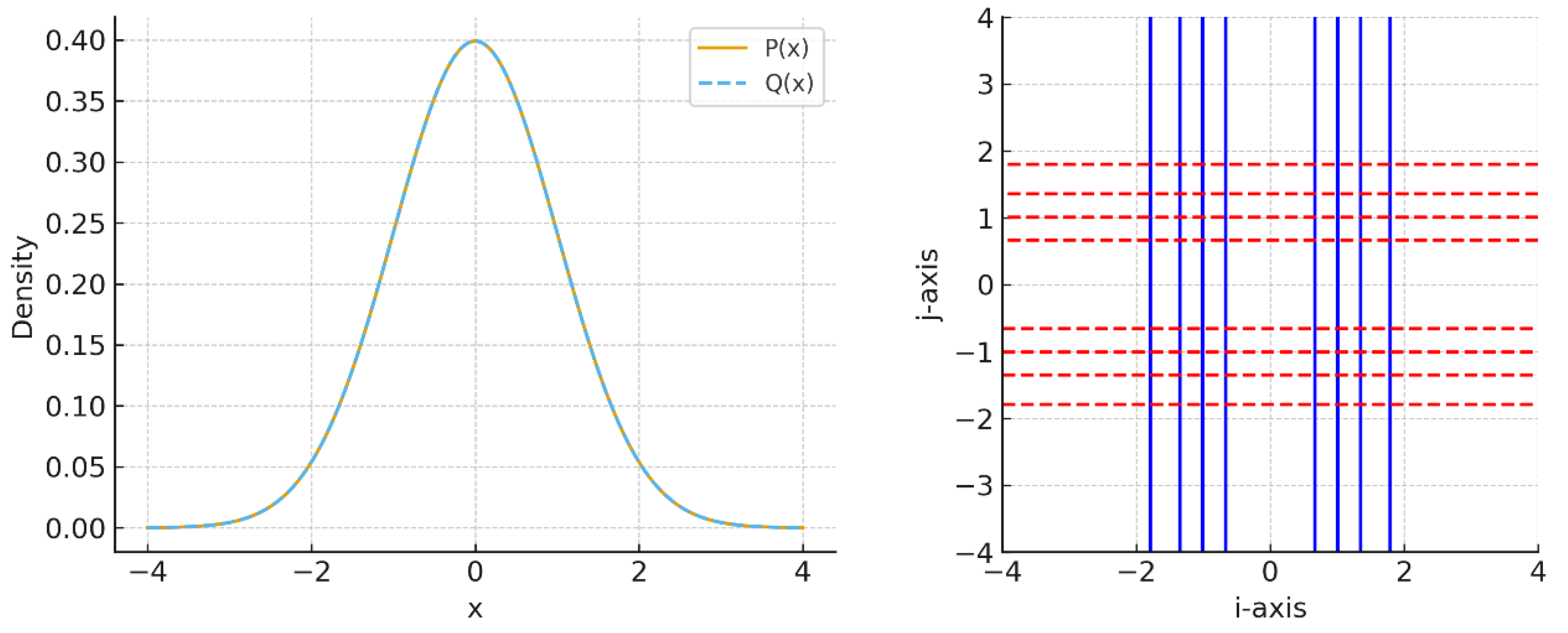
Example 12.5 — Divergence of orthogonal distributions.

  

Consider two distributions with the same scalar Gaussian density but orthogonal quaternionic orientations:

$$P\left(x\right)=\rho \left(x\right)\cdot i, Q\left(x\right)=\rho \left(x\right)\cdot j$$

Classically,

$$D_{KL}\left(P\parallel Q\right)=0,$$

so they are indistinguishable. Quaternionically,

$$D_{KL}\left(P\parallel Q\right)>0,$$

since $i$and $j$ are orthogonal.

As shown in Figure 5, the scalar view sees identical Gaussians, while the quaternionic view separates them as orthogonal distributions in phase space. This demonstrates the ability of quaternionic divergence to detect differences invisible to classical statistics.

13. Conclusion and Outlook.

This work introduces an axiomatic framework for quaternionic probability, extending Kolmogorov’s real-valued theory to measures and expectations taking values in $\mathbb{H}$ .The noncommutativity of quaternions manifests in two key ways: (i) left/right conditional probabilities and order-sensitive Bayes’ rules, and (ii) multiple, non-equivalent notions of independence (strong, left, right, scalar). We developed the associated calculus of random variables, expectation and variance, and we derived continuity and Fokker–Planck-type equations for quaternionic densities and currents. The framework accommodates quaternionic Markov chains and proposes a natural information theory separating scalar uncertainty from vectorial coherence.

The scalar projection recovers classical probability, while restriction to a complex subalgebra recovers complex (quantum-like) probability; yet several phenomena are strictly quaternionic, including order-dependent conditioning and phase-rotational transport in $SU\left(2\right)$. The examples show concrete scenarios where classical statistics is blind (identical scalars, zero KL) but quaternionic predictions differ in observables, divergences, or dynamics.

Future directions include: (1) law of large numbers and central limit theorems with vectorial coherence; (2) martingales, filtrations, and Doob-type results in quaternionic settings; (3) ergodic theory and spectral gaps for quaternionic Markov generators; (4) inference algorithms and estimation of quaternionic phases from data; (5) applications to spin-polarized transport, orientation-aware sensing, and order-effects in decision pipelines.

The examples presented in Section 12 highlight practical scenarios where quaternionic probability provides information that classical and even complex-valued frameworks cannot capture. In medical diagnostics, it naturally models order effects in sequential tests; in signal analysis, it reveals hidden coherence between orthogonal channels; in spintronics, it describes coupled diffusion and spin precession within a single law; in financial Markov chains, it encodes cyclical memory beyond scalar transitions; and in communications, it distinguishes channels with identical power spectra but different polarization states. These applications show that quaternionic probability is not only a consistent mathematical generalization but also a tool with concrete advantages in modeling systems where orientation, coherence, and order-dependence play a fundamental role.

Future directions include the exploration of connections between quaternionic probability and operator-algebraic approaches to noncommutative probability, its potential role in quaternionic quantum mechanics, and possible links with free probability and noncommutative geometry. These perspectives suggest that the present axiomatization may serve not only as a self-contained framework but also as a starting point for broader developments in mathematics and physics.

14. Numerical Methods and Reproducibility.

All figures were produced with Python and Matplotlib (no seaborn, one plot per figure, default color cycle). The code is deterministic and uses only elementary numerical routines. Source scripts are available upon request and can be deposited in a public repository.

• Computational environment.

• Language: Python 3.x; plotting: Matplotlib.
• No stochastic seeds are required; outputs are deterministic.
• Hardware: standard laptop; no GPU or special libraries.

15. Figure captions.

Figure 1. Left vs. right conditional probabilities. Both share the same scalar part but differ in their imaginary components, capturing order-dependent effects relevant in diagnostic testing.

Figure 1. Left vs. right conditional probabilities. Both share the same scalar part but differ in their imaginary components, capturing order-dependent effects relevant in diagnostic testing.

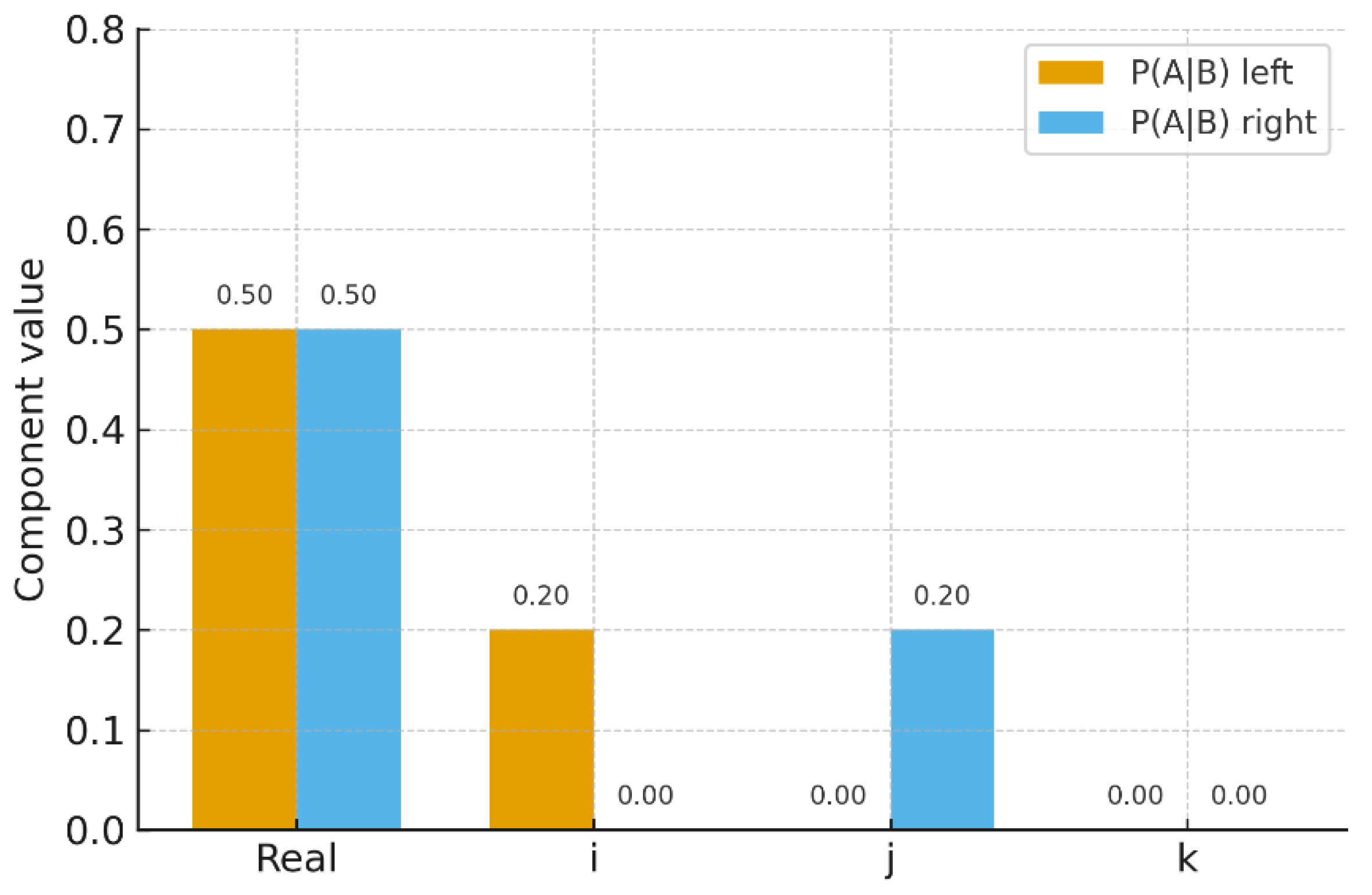
Figure 2. Classical vs. quaternionic correlation of sine and cosine signals. Classical covariance is zero (independence), while the quaternionic representation reveals perfect circular coherence.

Figure 2. Classical vs. quaternionic correlation of sine and cosine signals. Classical covariance is zero (independence), while the quaternionic representation reveals perfect circular coherence.

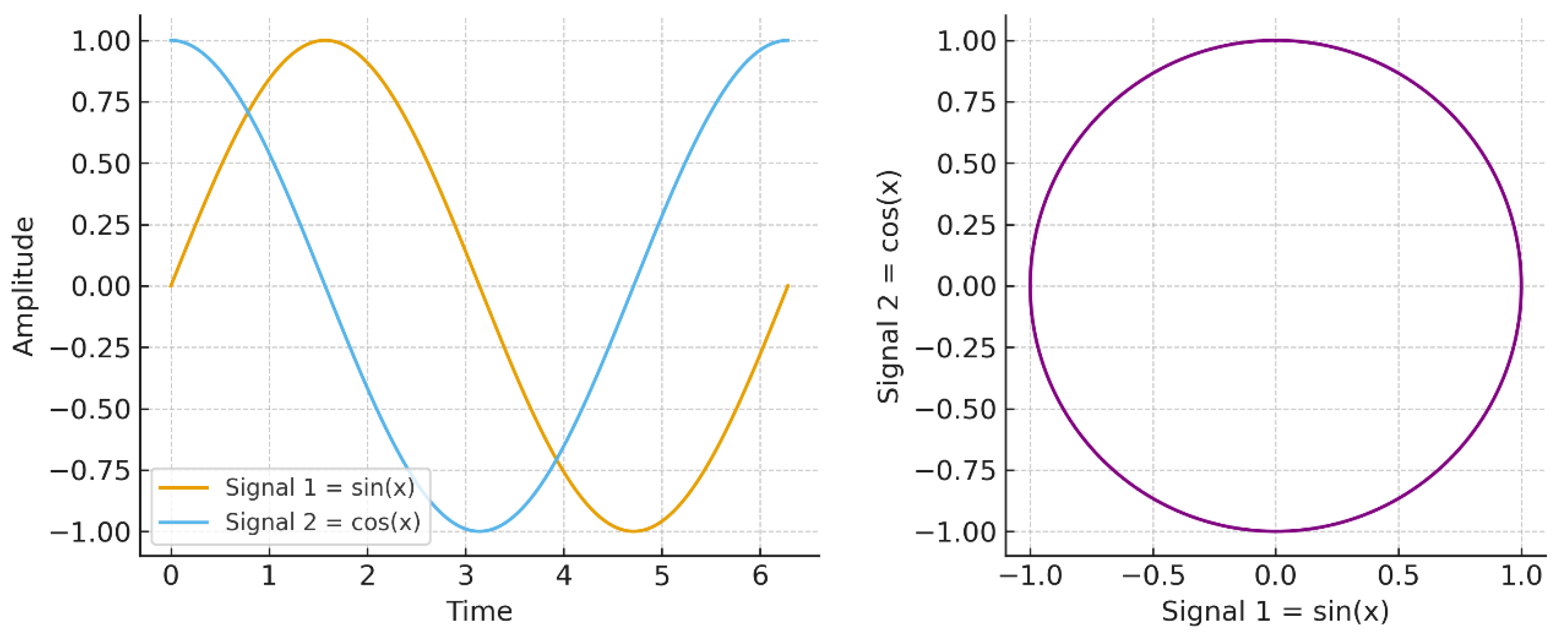
Figure 3. Scalar Gaussian diffusion at times $t=\mathrm{1,2},3$The scalar density broadens with time, while the quaternionic phase evolves, modeling coupled density–spin dynamics.

Figure 3. Scalar Gaussian diffusion at times $t=\mathrm{1,2},3$The scalar density broadens with time, while the quaternionic phase evolves, modeling coupled density–spin dynamics.

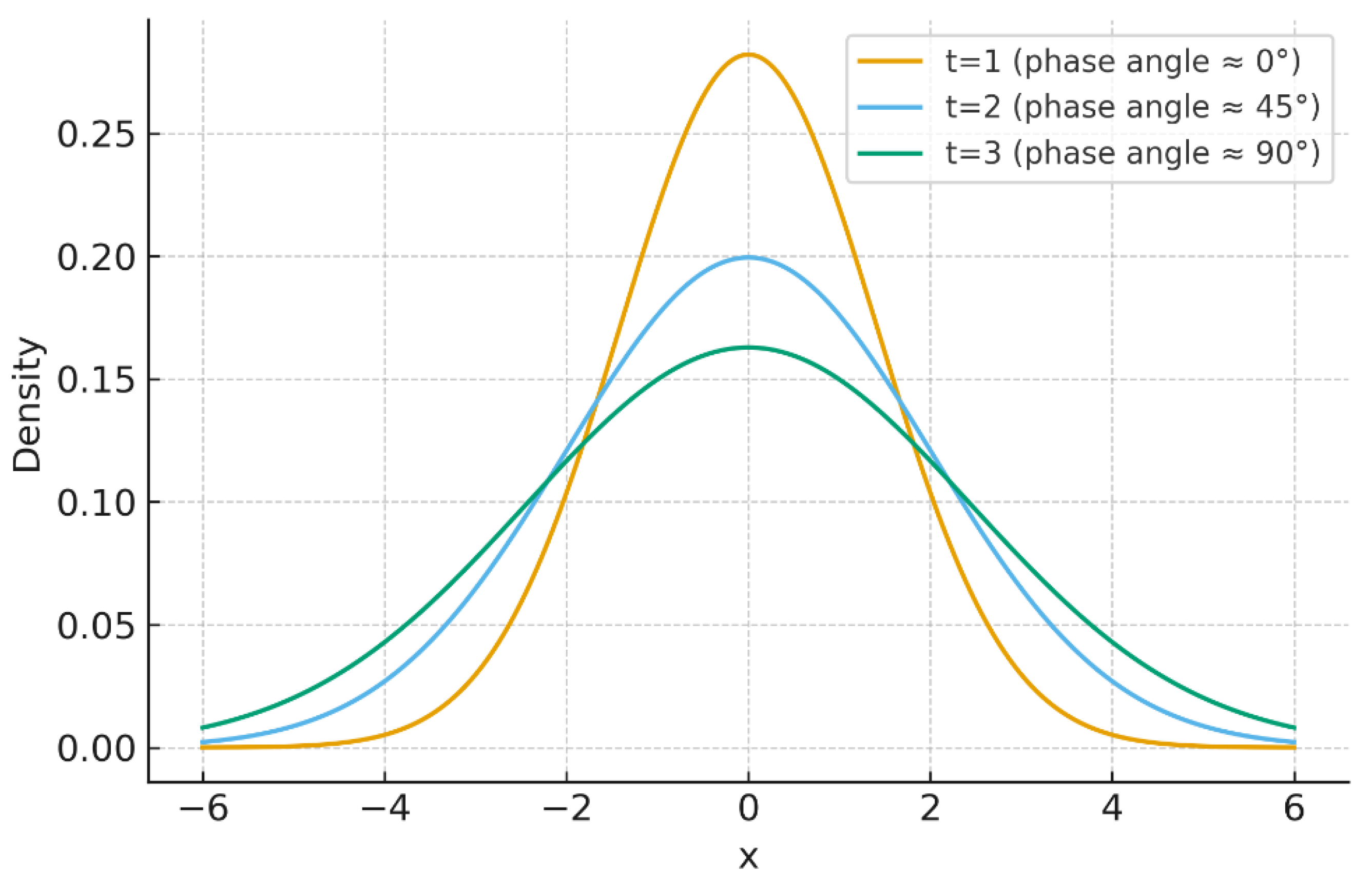
Figure 4. Two-state Markov chain. Classical probabilities alternate deterministically between states, while quaternionic evolution introduces a rotating phase, modeling cyclical memory effects.

Figure 4. Two-state Markov chain. Classical probabilities alternate deterministically between states, while quaternionic evolution introduces a rotating phase, modeling cyclical memory effects.

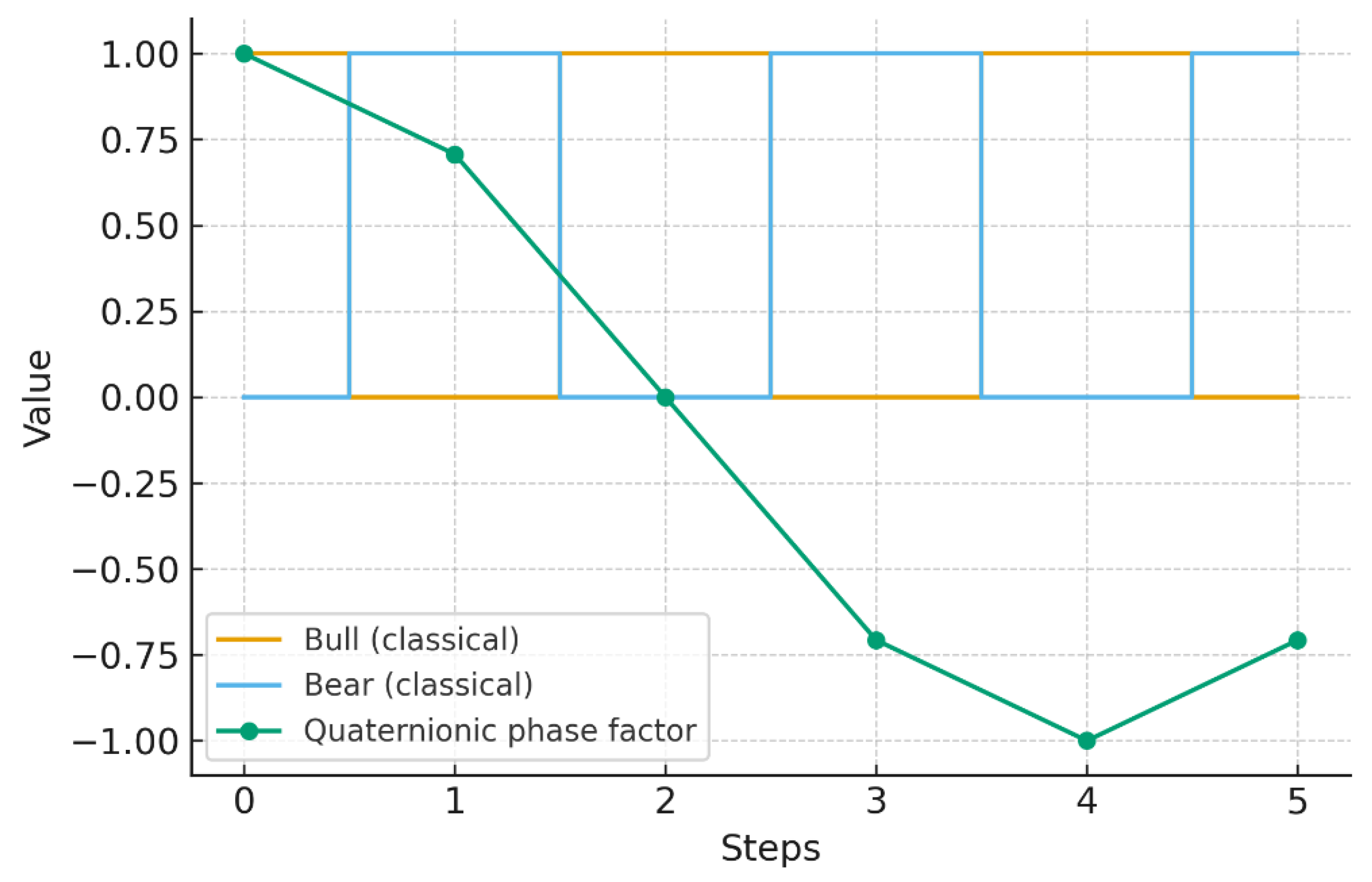
Figure 5. Scalar view: two identical Gaussian distributions, indistinguishable with classical KL divergence ${(D}_{KL}=0$). Quaternionic view: orthogonal orientations in phase space, yielding positive quaternionic divergence ($D_{\mathbb{H}}>0$).

Figure 5. Scalar view: two identical Gaussian distributions, indistinguishable with classical KL divergence ${(D}_{KL}=0$). Quaternionic view: orthogonal orientations in phase space, yielding positive quaternionic divergence ($D_{\mathbb{H}}>0$).

16. Technical Appendices

This appendix collects mathematical foundations and technical proofs that support the quaternionic probability framework.

16.1. Quaternionic measures

Definition A.1 (Quaternionic measure).

  

A function $\mu :\mathcal{F}\to \mathbb{H}$ is a quaternionic measure if:

• $\mu \left(\mathrm{\varnothing }\right)=0.$
• For pairwise disjoint $E_1,E_2,\dots \in \mathcal{F},$

$$\mu \left(\bigcup _{n=1}^{\infty }{E}_n\right)=\sum _{n=1}^{\infty }\mu \left(E_n\right),$$

with convergence in the quaternionic norm.

Lemma A.1 (Total variation).

  

Define the total variation of $\mu$ by

$$\left|\mu \right|\left(E\right)=\sup \left\{\sum _j|\mu \left(E_j\right) :\left\{E_j\right\} finite partition of E\right\}.$$

Then $\left|\mu \right|$ is a real-valued measure and $\mu$ is absolutely continuous with respect to $\left|\mu \right|$.

16.2. Quaternionic integration.

Definition A.2 (Bochner–quaternionic integral).

  

For a simple function $f=\sum _k{q}_k{\mu (E}_k)$​, define

$$\int fd\mu =\sum _k{q}_k{\mu (E}_k)$$

This extends by norm limits to all measurable functions $f:\Omega \to \mathbb{H}$.

Proposition A.1 (Norm inequality).

  

For any $f\in L^{-1}\left(\mu \right),$

$$\left|\int fd\mu \right|\le \int \left|f\right|d\left|\mu \right|$$

16.3 Functional calculus in$\mathbb{H}$.

• Exponential:

  $$e^q=\sum _{n=0}^{\infty }{\displaystyle \frac{q^n}{n!}}, q\in \mathbb{H}.$$
• Logarithm: defined on $\mathbb{H}\setminus (-\mathbb{\infty },0]$, with multiple values corresponding to directions in${\mathbb{S}}^3.$
• S-spectrum: For operators on quaternionic Banach spaces, the S-spectrum (Colombo–Sabadini–Struppa [22]) generalizes the classical spectrum and is essential for defining $e^{Qt}$ in Section 9.

16.4. Proof sketches.

• A.4.1 Bayes’ rules.

Noncommutativity requires distinguishing left and right multiplication. The denominator normalizes the scalar part to unity, ensuring consistency with Definition 3.1–3.2.

• A.4.2 Continuity equation.

Derived by integrating the balance law over regions and applying Gauss’ theorem componentwise.

• A.4.3 Fokker–Planck equation.

Obtained as a diffusion limit of jump processes with quaternionic increments, scaling $∆x^2~∆t$.

16.5. Summary.

• Quaternionic measures extend real measures consistently.
• The Bochner integral provides a rigorous foundation for expectations.
• Functional calculus guarantees the well-definedness of semigroups $e^{Qt}$.
• Proofs of conditional probability, continuity, and transport equations ensure mathematical coherence of the quaternionic framework.

This appendix secures the mathematical foundations of quaternionic probability, completing the proposed theory.

References

- Kolmogorov, A. N. (1933). Foundations of the theory of probability. Chelsea Publishing.
- Billingsley, P. (1995). Probability and measure (3rd ed.). Wiley.
- Doob, J. L. (1953). Stochastic processes. Wiley.
- Feller, W. (1968). An introduction to probability theory and its applications (Vol. 1, 3rd ed.). Wiley.
- Parthasarathy, K. R. (1967). Probability measures on metric spaces. Academic Press.
- Feynman, R. P. (1987). Negative probability. In B. J. Hiley & F. D. Peat (Eds.), Quantum implications: Essays in honour of David Bohm (pp. 235–248). Routledge.
- Khrennikov, A. (2009). Interpretations of probability. De Gruyter.
- Khrennikov, A. Classical and quantum mechanics on p-adic trees of ideas. Doklady Mathematics, 1999, 59, 450–452. [Google Scholar]
- Accardi, L. (1984). Non-Kolmogorovian probabilities and quantum physics. In Proceedings of the Conference on Mathematical Problems in Theoretical Physics (pp. 147–159). Springer.
- Accardi, L.; Cecchini, C. Conditional expectations in von Neumann algebras and a theorem of Takesaki. Journal of Functional Analysis, 1982, 45, 245–273. [Google Scholar] [CrossRef]
- Voiculescu, D. V. (1992). Free probability theory: Random matrices and von Neumann algebras. Proceedings of the International Congress of Mathematicians (pp. 227–241).
- Speicher, R. (2007). Lectures on free probability theory. Springer.
- Wysoczański, J. Non-commutative independence of algebras and applications to probability. Operators and Matrices, 2010, 4, 253–270. [Google Scholar] [CrossRef]
- Kümmerer, B. (1985). Markov dilations and noncommutative processes. In Probability measures on groups (pp. 216–236). Springer.
- Hamilton, W. R. (1853). Lectures on quaternions. Hodges and Smith.
- Sudbery, A. Quaternionic analysis. Mathematical Proceedings of the Cambridge Philosophical Society, 1986, 85, 199–225. [Google Scholar] [CrossRef]
- Adler, S. L. (1995). Quaternionic quantum mechanics and quantum field. Oxford University Press.
- Adler, S. L. (1996). Quaternionic quantum mechanics and noncommutative dynamics. arXiv preprint hep-th/9607008. https://arxiv.org/abs/hep-th/9607008.
Disclaimer/Publisher’s Note: The statements, opinions and data contained in all publications are solely those of the individual author(s) and contributor(s) and not of MDPI and/or the editor(s). MDPI and/or the editor(s) disclaim responsibility for any injury to people or property resulting from any ideas, methods, instructions or products referred to in the content. |
© 2025 by the authors. Licensee MDPI, Basel, Switzerland. This article is an open access article distributed under the terms and conditions of the Creative Commons Attribution (CC BY) license (http://creativecommons.org/licenses/by/4.0/).
Copyright: This open access article is published under a Creative Commons CC BY 4.0 license, which permit the free download, distribution, and reuse, provided that the author and preprint are cited in any reuse.