
Submitted:
09 September 2025
Posted:
25 September 2025
You are already at the latest version
Abstract
A shallow, seasonal snowpack is rarely homogeneous in depth, layer characteristics, or surface structure throughout an entire winter. Aerodynamic roughness length (z0) is typically considered a static parameter within hydrologic and atmospheric models. However, observations have shown that z0 is a dynamic variable, necessitating accurate spatial and temporal measurements of z0. Terrestrial LiDAR data were collected at nine different study sites in northwest Colorado from the 2019-2020 winter season to observe variability of the snowpack surface. Geometric z0 and snow depth (ds) observation over 112 site visits illustrated a change in z0 as a function of ds. Values of z0 decrease during initial snow accumulation, as the snow conforms to the underlying terrain. Once the snowpack is sufficiently deep, which depends on the height of the ground surface roughness features, the surface becomes more uniform. As melt begins, z0 increases, when the snow surface becomes more irregular. The correlation varied spatially and temporally though; it was obscured by snowpack surface modifications, such as the presence of vegetation, anthropogenic or ecologic influence. The rate of change in the z0 versus ds correlation was almost constant, regardless of the initial roughness conditions that only affected the initial z0.
Keywords:
aerodynamic roughness length
; hysteresis
; terrestrial LiDAR
; snow accumulation
; surface geometry
1. Introduction
A shallow seasonal snowpack covers approximately 50% of the Northern Hemisphere, making the snowpack surface the primary land-atmosphere interface during the winter season [1,2]. Across Colorado United States (U.S.), an important headwater state in the western United States, 60% of annual precipitation falls as snow [3,4]. Accurate observations and modeling of snow water resources in the western United States is essential for water budgeting, recreation, wildfire management, and ecological resources [5].
The snowpack varies spatially and temporally [6], and is controlled by local, regional, and global weather and climate [7]. Consequently, snowpack conditions will vary between maritime and continental climates [8]. Due to the variability of the snowpack across these various regimes, a standard metric to quantify the snowpack is difficult to acquire. The aerodynamic roughness length, , can be used as a measure of the snowpack surface [9,10]. The captures the variability that is produced by land cover characteristics as well as the underlying topography [2,6,11]. The variability is further enhanced by meteorological conditions [6], non-uniform distribution of snow cover during accumulation and ablation [6,9], snow-canopy interactions [12], and wind redistribution of snow [13]. Small scale (<1 meter) and large scale (>1 meter) variations within the snowpack can alter the overall value [10,14,15]. The effect of a single roughness feature coupled with non-uniform spatial arrangement among other elements affects all aspects of the snowpack surface [9,10]. A dynamic characterizes heterogeneity in snow-water equivalent, melt rates [9], redistribution, snow deposition [6], and surface energy fluxes [16].
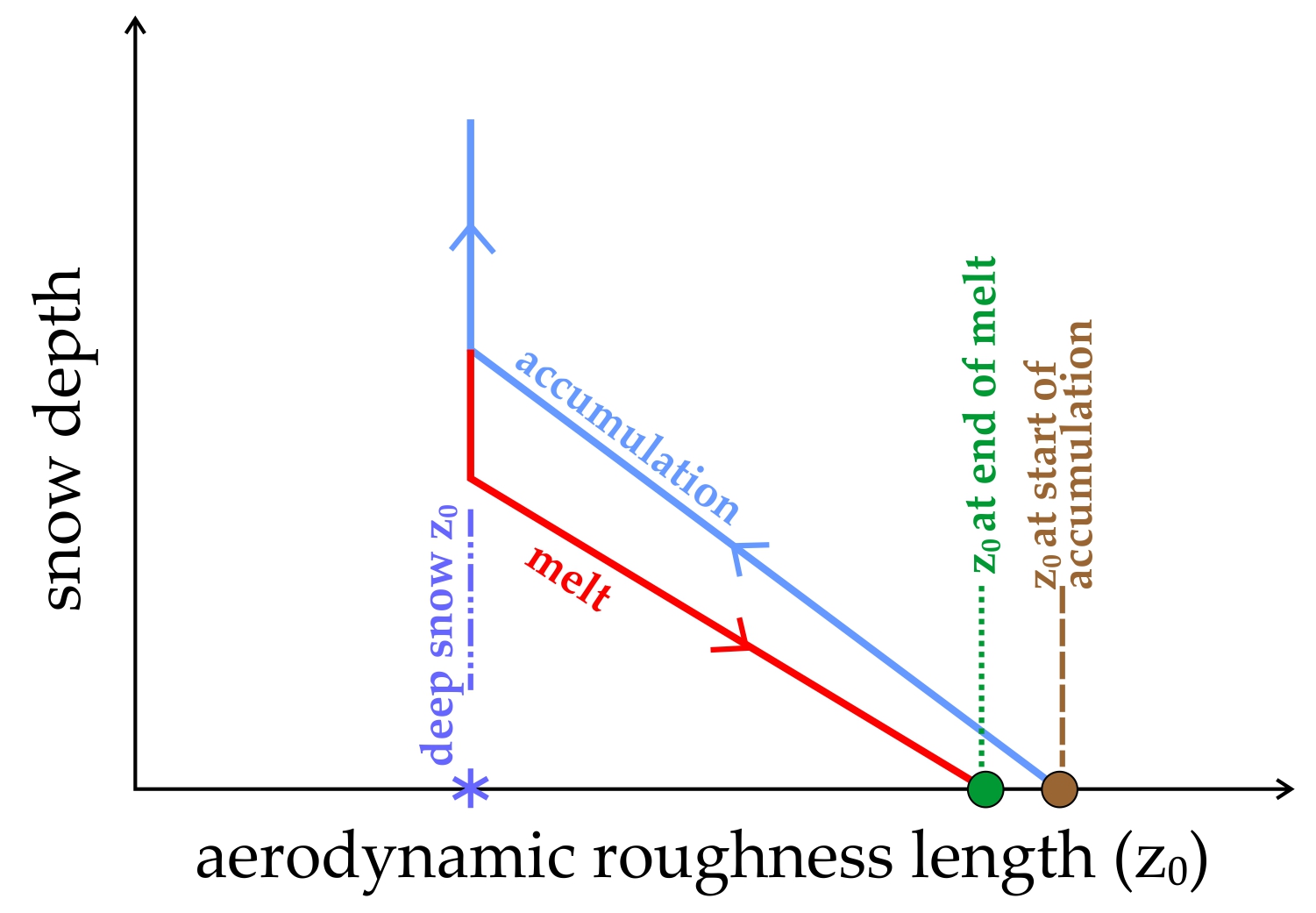
The will decrease during accumulation as the snow initially conforms to the underlying terrain (Figure 1) [16]. Once a threshold snow depth, , is reached, the snow surface has decoupled from the topography and becomes smoother, resulting in a smaller [9,16,17]. Quincey et al. [18] found that one new snowfall decreased by 75% since it covered small scale feature variability and only large features were left to increase the roughness. As decreases due to compaction, metamorphism and/or ablation, ground-based surface features and underlying topographical features are re-coupled with , increasing its variability [16,19].
This relation of increasing and decreasing in some form has been observed previously [2,9,20]. This correlation of and is not considered within hydrologic, snowpack, or land surface models. The relation of these two factors is also expected to differ between periods of melt and accumulation as periods of melt are typically less uniform [16]. Swenson and Lawrence [21] found that topography and land cover features have the most influence on the hysteresis. Once the snow cover has reached full coverage over these features, the snowpack will accumulate homogeneously [16]. These early, mid, and late-season snowpack surface changes have important impacts (Figure 1) on estimating an accurate value within hydrologic models [19].
To accurately understand and model the snowpack, variability needs to be considered at the local level. Otherwise, hydrologic models will either over or underestimate melt water availability and melt rates [19,22,23]. Currently, the same is used for an entire watershed, based on the assumption of 100% snow covered area, undeviating melt throughout an area, despite the topographic or vegetation influences [6,23]. No other spatial or temporal variation in are represented [24]. Therefore, we hypothesize that the incorporation of as a dynamic variable, rather than a static parameter, will improve meteorologic, snowpack and hydrologic models [2,19,20,23,25]. To understand and observe the relation between and , the following questions are asked: 1) Does the snow surface roughness, defined here as , change as a function of ? 2) Does the correlation between and vary over space? 3) Is the decrease in as increases consistent regardless of the initial ground roughness? 4) Is the correlation between increasing and decreasing snow surface a function of the initial roughness feature, such as dominate vegetation and topographic features? and, 5) Is there a difference between the - correlation during periods of accumulation and melt, i.e., is it a hysteretic?
2. Data and Methods
2.1. Site Descriptions
Sites were selected based on varying topography, vegetation cover and abundance, elevation, and distribution throughout the watershed. This aided in determining spatial differences and the versus correlation. We selected nine sites near Meeker, Colorado (Figure 2), with an elevation range from 1,885 to 2,468 meters, to evaluate the research questions. Land cover ranged from open, grassy fields to large Pinyon-Juniper and shrub dominated sites. Sites were chosen for land cover variability, size of the primary roughness feature, and winter accessibility (Table 1). Annual precipitation ranges from 391 to 631 millimeters [26].
Each site was equipped with a Bluetooth Blue Maestro Tempo Disc sensor [27] that recorded hourly temperature, humidity, and dew point temperature. Three or four T-posts were installed with measuring tape to record . A silver sphere was added to the north facing T-post for direction orientation.
2.2. Field Data Collection
The snowpack surface was measured using a FARO Focus3D X 130 model Terrestrial LiDAR Scanner (TLS) [28]. This LiDAR instrument generates a point cloud scan of a given area with an error of +/- 2 millimeters and a resolution of approximately 7.5 millimeters. Three LiDAR scans from different locations were taken during each site visit to avoid shadowing from roughness features. TLS scan frequency ranged from every two days to monthly. Scan interruptions occasionally occurred due to extreme winter weather and/or inability to reach the site safely.
During each site visit, the Blue Maestro [27] air temperature () and relative humidity data were downloaded. The current weather conditions (sunny, cloudy, windy, etc.), upcoming storm forecasts, approximate new snow accumulation, snow depths at each T-post were recorded. Photos were taken of the site. These data and photos were used to explore any inconsistencies among the calculations, or processing errors. Meteorological data () were used to explore any major temperature warming or cooling that may have altered melt rates.
2.3. Data-Processing
The three LiDAR scans from each site visit were cropped, merged, and aligned with each other in the corresponding cardinal direction (Figure 3) in the open-source program Cloud Compare [29]. An area of interest (AOI) was chosen for each site within the middle of the t-posts that varied in size from 2x2 m to 8x8 m, and typically included a primary roughness feature such as a sagebrush or shrub (Figure 2). The AOI had a resolution from 1 to 10 millimeters for a total of approximately 1.3 million points. The AOI was cropped out of each merged/aligned scan and interpolated using kriging at a 0.01-meter resolution in the Golden Software Surfer [30]. This created an interpolated, gridded AOI that was de-trended [11] in the x-y plane to remove the bias from the slope of the field or the angle of the LiDAR scanner [20].
For the AOI, the final geometric was calculated using the general approach of Lettau [31], specifically with the discretization and numerical method and code from Neville et al. [15]. This is a MATLAB code to apply Lettau’s equation to identify the mean obstacle height, , by finding all local maxima and minima relative to each other across the surface. Then, the lot area, S, is calculated as the total area divided by the total number of maxima. Next, the silhouette area, s, is found as the profile of an obstacle, this is done at a predefined resolution step. These steps, applied within equation (1), results in the average of the surface:
Note that Lettau [31] divides equation (1) by 2, but Sanow et al. [20] found that halving was unnecessary.
The for each LiDAR scan were calculated using Cloud Compare [29] by subtracting the initial snow-free scan from the snow-covered scan (Figure 3). The mean were computed across the AOI. Snow depths from site visits were cross-evaluated against LiDAR point clouds to ensure accuracy during post-processing. The snow depth observations at each T-post were also used to assess the LiDAR-derived snow depth estimate.
2.4. Data Analysis
Initial roughness LiDAR scans were taken with no snow on the ground. When snow was present throughout the season, the initial scans were subtracted from the snow-covered scans to find the average . The corresponding values were calculated for each scan, including those with and without snow.
Resulting snow depths were plotted against the natural logs of for each site and grouped by slope. The coefficient of determination () was found for each site. One site, Julie Circle, was chosen to observe the hysteresis between periods of accumulation and melt due to the high temporal frequency of scans Table 1. Melt versus accumulation was determined by of the previous scan. If had increased since the last scan, it was an accumulation time step. If it had decreased, it was a melt time step. This was verified using site photos as well as recorded hand measurements.
3. Results
Over the 2019-2020 winter season, 112 total site visits were conducted between October and April. All sites, except Lost Creek (Figure 4c), showed that as increased and enveloped roughness features, the corresponding decreased (Figure 4). For example, the Piceance site (P in Figure 4b) shows increasing and the corresponding decreasing in until 3 March 2020, when melt began. Furthermore, as starts decreasing, the values begin to increase. This relation developed quickly, and roughness feature size had an impact on the trend line slope. Lost Creek was disturbed during the spring and therefore did not follow this same temporal pattern (Figure 4c and Figure 5a,b).
To identify spatial and temporal patterns, the sites were grouped using the resulting slopes from the least square regression fit: CR11, Julie Circle, and Trout Farm (Figure 4a); Cathedral Creek, Piceance, Spring Creek, and Upper Piceance Creek (Figure 4b); Lost Creek (Figure 4c); and Yellow Jacket (Figure 4d). CR11 and Julie Circle have similar values (0.73 and 0.68, respectively), slope, roughness feature height, and initial values (Figure 4a). This result was seen despite the difference in data quantity between the two sites, i.e., five measurements (CR11) versus 31 measurements (JC). The primary roughness feature height (height of the tallest feature found within the AOI Table 1) at CR11 and Julie Circle are 0.46 m and 0.35 m; the slope is -0.048 and -0.043, respectively. Julie Circle had one notable outlier on 6 February 2020, with a of 0.52 m and a value of 3.5 x m (Figure 6). This occurred after an overnight storm deposited 0.18 m of new snow. Conversely, the lowest at the site occurred on 10 February 2020 with a of 0.41 m and a of 0.25 x m. Similar to Julie Circle, the deepest at CR11 of 0.49 m on 10 February 2020 had a of 0.18 x m, yet the lowest ( of 0.07 x ) at the site occurred during the second deepest of 0.43 m on 29 January 2020. Trout Farm had a similar slope to this pair (Figure 4a). Yet, compared to CR11 and Julie Circle with initial values of 66 x m and 40 x m, Trout Farm had the lowest roughness feature height (0.01 m for a grassy lawn) and initial of 4.8 x m (Figure 5c,d. These initial values are an order of magnitude different between CR11 and Julie Circle. However, the slope of -0.02 at Trout Farm was not substantially different from Julie Circle.
The second grouping of sites includes Cathedral Creek, Piceance, Spring Creek, and Upper Piceance Creek (Figure 4b). These sites had the lowest number of site visits (three to eight) due to distance and difficult winter access. The slopes of all four sites were alike, Cathedral Creek -0.15, Piceance -0.11, Spring Creek -0.13, and Upper Piceance Creek -0.14. The main variation among these sites is the , primary roughness feature height, and initial values. Spring Creek and Upper Piceance Creek have the highest of 0.71 and 0.79, respectively. Though, Spring Creek had the least amount of site visits and corresponding data. Upper Piceance has the highest amount of site visits in this grouping. Outliers from Cathedral Creek are from the two highest of 0.19 m and 0.23 m, and values 4.9 x m and 4.4 x m, respectively. Furthermore, the second group had the largest variation of roughness feature sizes ranging between 0.68 m at Piceance and 1.65 m at Upper Piceance Creek. It was initially thought that Piceance would correlate with group a (Figure 4a) due to the size of the primary roughness feature height. Yet, the initial was 1.1 x m, which is much larger than the others within group a.
Spring Creek had a roughness feature height of 1.1 m and initial of 2.2 x m which represents an average throughout the sites. The all-site average slope, roughness feature size, and initial was -0.10, 0.84 m, and 1.9 x m, respectively. Cathedral Creek had the highest initial value of 5.6 x m, but it had only the third largest roughness feature (1.3 m), indicating the site had the highest quantity of roughness features. Upper Piceance Creek had the second-largest initial value and roughness feature height at 3.9 x m and 1.65 m, respectively. However, both sites fell below Yellow Jacket, which was placed singularly into Figure 4d. Yellow Jacket had the largest roughness feature of 1.85 meters (Aspen, large sage, and shrubbery). Though, it produced the third largest initial value of 3.3 x m. Additionally, it had the steepest slope of any of the sites at -0.32. Yellow Jacket had two outliers that resulted in a higher value than the initial value. These instances occurred on 16 March 2020 and 7 April 2020, late in the season after peak had occurred (Figure 5e,f).
Lost Creek experienced heavy anthropogenic influence as shown in Figure 4c. Between 28 January and 26 February 2020 a snowmobile drove through the site which altered the natural progression of the snow (Figure 5a,b). Still, Lost Creek results show some similarities to the other sites. Prior to the snowmobile, Lost Creek was following the same hysteresis relation as the other sites. Lost Creek had the lowest , -0.28, attributed to the data being forced through the origin on the plot. When the data is not forced, the becomes 0.08, which is still a very low correlation likely due to the snowmobile tracks.
Since Julie Circle had the most data points of any site, it was used to analyze melt and accumulation values (Figure 6). There are 12 accumulation points, 17 melt points, and two points with of 0 m, taken as the initial surface roughness scan (fall) and the final surface roughness scan (spring). The results had a varying slope of -0.03 for melt, and -0.04 for accumulation. Melt resulted in an of 0.36, and accumulation resulted in an of 0.66.
4. Discussion
The calculated changed as a function of observed , although outliers of the relation existed. The first outlier was at the Julie Circle location (Figure 4a). The initial point on the x-axis indicates the highest value (40 x m) due to the lack of snow, i.e., = 0 and this occurred prior to accumulation. The other point with a of 0 was at the end of the season after all the snow melted produced less than half the (16 x m)of the initial . This is likely attributed to the vegetation type, which is a regular lawn grass that was pushed down by the weight of the snow throughout the year. This scenario could happen to any type of thin, flexible vegetation, fluctuating values depending on time of year [10,18].
Another discrepancy at the Julie Circle site is the lack of correlation between the highest and lowest value. A likely explanation for this observation is the large Cottonwood tree that overhangs the Julie Circle site. For example, within the point clouds the pock-marks in the snowpack surface (Figure 3b) where accumulated canopy snow fell from the limbs and altered the roughness. No other sites in this study had canopy cover like Julie Circle. Although, most sites did have shrubbery present [32], so even small-scale canopy interception and deposition was possible [18]. Canopy interception and redeposition is a potential issue when correlating between and . Therefore, to assume a uniform or linearly metamorphosing or melting snowpack could lead to errors [9,10,33].
This lack of correlation is also noted at CR11 and Trout Farm. Similar to Julie Circle, the highest value did not correspond with the lowest value at CR11. This can be attributed to a recent snowfall event of about 10 cm that had fallen the day before the 29 January 2020 scan. On 10 February 2020 there was less fresh snow (approximately 5 cm) and conditions were sunny and warm. These differences in the snowpack were recorded in site notes and photos from the visits. Likewise, Trout Farm also experienced the same contradiction, the highest value had a greater than double the lowest calculated . This indicates that these small variations of the snowpack surface is key to addressing beyond simply considering the snow depth. Accounting for small surface variations is especially important on flat sites where initial may be surpassed by the development of surface features such as sun cups, sastrugi, surficial features, wildlife, and anthropogenic modifications [4,18,33,34].
Cathedral Creek (Figure 4b), followed the and relation until the 10 and 24 February 2020 scans. Between the scan dates of 16 January and 10 February 2020 temperatures were often warmer than , with a maximum temperature of 19°C. The interpolated surfaces of 16 January 2020 (lowest ) and 24 February 2020 (highest ) are shown in Figure 7, highlighting pock-marks and uneven melting. These elevated temperatures resulted in an increased, non-uniform melt [9]. So, even though additional snow fell between the scans, it did not completely cover the snow surface characteristics [9,16,17].
Yellow Jacket had the highest initial of any of the sites (Figure 4c). Photos from the field visits late in the season show a lot of recent melt, which revealed larger shrubs as well as the development of sun cups within the AOI (Figure 4e,f). The late season increase in roughness likely produced two irregular points with a higher than the initial after peak had occurred [2]. Another influence on the site was the anthropogenic modifications of snowmobile tracks. Combining these two factors led the roughness variations to be larger than the initial grassy, shrub-filled plot. This same anthropogenic disruption occurred at the Lost Creek site (Figure 4c and Figure 5a-d). This led to an extreme increase in after the disturbance, even with the deep snowpack 0.85 m (Figure 4d). The large increase in at the site was exacerbated by the very flat topography that contained one small, controlled roughness feature (railroad tie) in the middle.
We hypothesized that slopes would remain the same and the x-intercept would change. However, the initial ground roughness played a critical role in the slope of the data. The 0.13 meter railroad tie at the Lost Creek site is an example of a feature responsible for the initial site value of 9.4 x m. Without it, the would have been lower as the site was an open, grassy field. Due to this controlled roughness feature, none of the snowmobile-caused values were larger than the initial . Lost Creek also had some of the highest , which led to higher values, especially coupled with snowmobile tracks. Snowmobiling and other recreational activities are common throughout public lands during the winter [4]. Anthropogenic factors such as these are important to consider when evaluating a spatially and temporally dynamic [4]. Moreover, this could explain the discrepancies in sites like Yellow Jacket, also influenced by snowmobiles. Together, land cover type and function need to be considered when applying [4].
Figure 4b shows the grouping of Cathedral Creek, Piceance, Spring Creek, and Upper Piceance Creek. The slopes of all four sites were similar ranging from -0.11 to -0.15. The values, roughness features (ranging between 0.68-1.65 meters), and initial values (ranging from 1.1 to 5.7 x m) varied among the sites. Based on the primary roughness feature heights, Piceance aligns with the CR11, Julie Circle, and Trout Farm group than the one in which it was placed. Upper Piceance was more similar in initial and roughness feature size to Yellow Jacket, but their slopes have a difference of 0.17. However, as discussed, there were some values that skewed the slopes in these sites. Potential reasoning for this was noted at several sites, such as overall changes of the surface of the snowpack throughout the season due to wind redistribution [35], surface energy fluxes [9], formation of surface features [2], and non-uniform melt and accumulation [9]. These influences metamorphize the snowpack and are very difficult to quantify or predict. The development of surface features is one reason why the slopes of Trout Farm and Julie Circle have only a slight difference despite the initial values being an order of magnitude different (4.8 x and 40 x m, respectively).
Julie Circle was used to compare melt and accumulation values (Figure 6). The accumulation values had a stronger value of 0.66, compared to that of the melt ( = 0.36), indicating accumulation was more uniform [16] (Figure 1). This was to be expected, since this relation was not observed to be linear in either case. The low correlation of the melt values can be attributed to several environmental processes, which is typically occurs within any snowpack. Potential melt factors are sensible and latent heat fluxes, dust deposition [36], spatial and temporal distribution of incoming solar radiation [37], wind redistribution [33,39], longwave radiation [38], anthropogenic alterations [4,13], air temperature [40], spatial heterogeneity of the snowpack [23], and vegetation cover [7]. Since melting occurred throughout the season, the environmental influences were also affecting accumulation rates, which supports the heterogeneity of the accumulation values. Melt rates influence atmospheric and hydrologic processes [13], and understanding the processes and rates that control melt water production is important for predicting the timing and magnitude of peak melt in a watershed [22,23,41]. Initially, accumulation versus melt hysteresis aspect of the study was to be conducted at Lost Creek and Yellow Jacket, however, these sites were anthropogenically altered and were thus not used. It was hypothesized that the melt versus accumulation at Yellow Jacket would yield a higher difference between the accumulation slope and the melt slope due to the higher initial roughness and quantity of roughness features to enhance melt (Figure 5e and f). Since Lost Creek was a flat, open site (Figure 5a), it was hypothesized that the slopes would be similar to Julie Circle. The primary influence of melt at Julie Circle was the addition of ecological factors from the tree near the site, and the proximity to a residential house, potentially increasing the effects of longwave radiation induced melt. At Lost Creek, incoming solar radiation would dominate snowmelt. Therefore, slopes even more similar to each other were expected.
The method used to determine melt compared to accumulation values is also a source of potential error. Settling and metamorphism of the snowpack could have occurred resulting in snow depth decreases without any actual snowmelt taking place [13,16,37]. Photos, atmospheric conditions, and visual assessments of the site were completed. For these shallow snowpacks where multiple melt cycles can occur, snow wetness sensors, soil moisture sensors, and other atmospheric/hydrologic monitoring equipment could aid in determining the exact periods of melt. In deeper snowpacks, that typically only have one melt period at the end of the winter, within snowpack temperature sensors could assist in determining when the snowpack becames isothermal and is being to melt.
4.1. Next Steps
This study consisted of 112 site visits, which produced a robust dataset for observing trends and correlations. While increased temporal scan frequency, preferably daily, would offer further insight into the snowpack surface evolution due to surface processes [6,7] and meteorological factors [2,40], the current dataset still captures the overall temporal changes. The scan areas represent a small portion of the White River watershed. Although this limits direct watershed-scale extrapolation, the findings highlight important local-scale processes and variability. Site-specific features, such as the cottonwood tree at Julie Circle which influenced surface conditions and canopy cover, reflect natural heterogeneity common in snow-covered landscapes [16]. However, some consistency was observed between sites with similar terrain and land cover. For example, Upper Piceance Creek and Cathedral Creek, both are situated on old river terraces near cliffs, exhibited comparable initial roughness values (39 x and 56 x m) and similar feature heights (1.65 m and 1.3 m), producing nearly identical versus slopes (-0.15). This suggests that once a versus correlation is identified, it could be applied to other areas with similar characteristics.
Future studies could include larger plots within a smaller watershed that can be scanned with LiDAR for snow accumulation and melt more frequently [16,20]. Measuring and/or modeling meteorological data, such as (net) shortwave and longwave radiation, could provide more insight to determining melt periods and subsequent accumulation periods during mid and late season melt [36,37]. This could yield a change in one of or without a change in the other, i.e., hysteresis between blue and red lines in Figure 6 [42]. This study is a step toward understanding snowpack surface roughness dynamics and scaling roughness-based energy balance assessments, which will improve snowpack, hydrological and meteorological modeling [2,19,20,23].
Furthermore, future studies could explore errors of uncertainty within the calculations. The current code [15] calculates based on the local maxima and minima within the scan area. This method is acceptable when roughness elements are homogenously spaced and sized, however, that is not always the case in nature. The code could be reformed to calculate on a certain sized area (every 0.012 meter, or 0.12 meter, etc. depending on the size of the scan). This would give a distribution of values that would encompass the variations in terrain, vegetation, size, and/or distribution of roughness characteristics. This methodology could enhance the estimation of for an area that is larger, as a larger area (>100 m) will tend to have more variations than a small area (<10 m), such as sites used within this study.
5. Conclusions
At all study locations, it was observed that as increased decreased. This correlation varied spatially and was dependent on the initial roughness of the site. Initial roughness features played a large role in determining the slope and x-intercept of the versus correlation. Although, when sites are disturbed during the course of data collection, the variability of can change by orders of magnitude, as observed several sites. Hence, the use in an area changes the correlation. We observed hysteresis between the versus correlation from periods of melt and accumulation.
Author Contributions
Conceptualization, J.E.S. and S.R.F.; methodology, J.E.S. and S.R.F.; software, J.E.S.; formal analysis, J.E.S.; investigation, J.E.S. and S.R.F.; data curation, S.R.F.; writing—original draft preparation, J.E.S. and S.R.F.; writing—review and editing, J.E.S. and S.R.F.; visualization, J.E.S. and S.R.F.; supervision, S.R.F.; project administration, S.R.F.; funding acquisition, J.E.S. and S.R.F. All authors have read and agreed to the published version of the manuscript.
Funding
This research was indirectly funded by the U.S. Geological Survey National Institutes for Water Resources (U.S. Department of the Interior), grant number 2019COSANOW, project “The Dynamic Nature of Snow Surface Roughness”, through the Colorado Water Center at Colorado State University. This material is based upon work supported by the National Science Foundation under Grant No. DMS-1615909.
Institutional Review Board Statement
Not applicable.
Informed Consent Statement
Not applicable.
Data Availability Statement
We are in the process of publishing the TLS LIDAR scans online at https://doi.org/10.5061/dryad.80gb5mm35
Acknowledgments
Not applicable.
Conflicts of Interest
The authors declare no conflicts of interest.
References
- Mialon, A.; Fily, M.; Royer, A. Seasonal snow cover extent from microwave remote sensing data: Comparison with existing ground and satellite based measurements. EARSeL eProceedings 1994, 4, 215-225.
- Fassnacht, S. R.; Williams, M. W.; Corrao, M. V. Changes in the surface roughness of snow from millimetre to metre scales. Ecological Complexity 2009, 6 (3), 221–229. [CrossRef]
- Barnett, T.P.; Pierce, D.W.; Hidalgo, H.G.; Bonfils, C.; Santer, B.D.; Das, T.; Bala, G.; Wood, A.W.; Nozawa, T.; Mirin, A.A.; Cayan, D.R.; Dettinger, M.D. Human induced changes in the hydrology of the western United States. Science, 2008, 319(5866), 1080-1083. [CrossRef]
- Fassnacht, S.R.; Heath, J.T.; Venable, N.B.H.; Elder, K.J. Snowmobile impacts on snowpack physical and mechanical properties. The Cryosphere, 2018a, 12, 1121-1135. [CrossRef]
- Fassnacht, S.R.; Venable, N.B.H.; McGrath, D.; Patterson, G.G. Sub-seasonal snowpack trends in the Rocky Mountain National Park area, Colorado, USA. Water, 2018b, 10(5), 562 . [CrossRef]
- Niu, G. and Yang, Z.L. An observation-based formulation of snow cover fraction and its evaluation over large North American river basins. Journal of Geophysical Research, 2007, 112(D21). [CrossRef]
- Anttila, K.; Manninen, T.; Karjalainen, T.; Lahtinen, P.; Riihela, A.; Siljamo, N. The temporal and spatial variability in submeter scale surface roughness of seasonal snow in Sodankyla Finnish Lapland in 2009-2010. Journal of Geophysical Research: Atmospheres, 2014, 119, 9236-9252. [CrossRef]
- Trujillo, E. and Molotch, N.P. Snowpack regimes of the Western United States. Water Resources Research, 2014, 50, 5611-5623. [CrossRef]
- Luce, C. H. and Tarboton, D.G. The application of depletion curves for parameterization of subgrid variability of snow. Hydrological Processes, 2004, 18(8), 1409–1422. [CrossRef]
- Smith, M.W. Roughness in the earth sciences. Earth Science Reviews 2014, 136, 202-225. [CrossRef]
- Fassnacht, S. R.; Stednick, J. D.; Deems, J. S.; Corrao, M. V. Metrics for assessing snow surface roughness from digital imagery. Water Resources Research 2009, 45, W00D31. [CrossRef]
- Moeser, D.; Stahli, M.; Jonas, T. Improved snow interception modeling using canopy parameters derived from airborne LIDAR data. Water Resources Research, 2015, 51(7), 5041-5059. [CrossRef]
- Liston, G.E. Representing subgrid snow cover heterogeneities in regional and global models. Journal of Climate, 2004, 17(6), 1381–1397. [CrossRef]
- Blöschl, G. Scaling issues in snow hydrology. Hydrologic Process, 1999, 13, 2149-2175. [CrossRef]
- Neville, R.A.; Shipman, P.D.; Fassnacht, S.R.; Sanow, J.E.; Pasquini, R.; Oprea, I. A geometric-based aerodynamic roughness length formulation and code applied to lidar-derived snow surfaces. Remote Sensing, 2025, 17(2). [CrossRef]
- Magand, C.; Ducharne, A.; Le Moine, N. Introducing hysteresis in snow depletion curves to improve the water budget of a land surface model in alpine catchment. Journal of Hydrometeorology, 2014, 15(2), 631–649. [CrossRef]
- Brock, B.; Willis, I.; Sharp, M. Measurement and parameterization of aerodynamic roughness length variations at Haut Glacier d’Arolla, Switzerland. Journal of Glaciology 2006, 52 (177), 281–297. [CrossRef]
- Quincey, D.; Smith, M.; Rounce, D.; Ross, A.; King, O.; Watson, C. Evaluating morphological estimates of the aerodynamic roughness of debris covered glacier ice. Earth Surface Processes and Landforms, 2017, 42, 2541-2553. [CrossRef]
- Manes, C.; Guala, M.; Löwe, H.; Bartlett, S.; Egli, L.; Lehning, M. Statistical properties of fresh snow roughness. Water Resources Research, 2008, 44(11), 1–9. [CrossRef]
- Sanow, J.E., Fassnacht, S.R., Kamin, D.J., Sexstone, G.A., Bauerle, W.L., Oprea, I. Geometric versus anemometric surface roughness for a shallow accumulating snowpack. Geosciences 2018, 8(12), 463. [CrossRef]
- Swenson, S.C. and Lawrence, D.M. A new fractional snow-covered area parameterization for the Community Land Model and its effect on the surface energy balance. Journal of Geophysical Research, 2012, 117(D21). [CrossRef]
- Luce, C.H.; Tarboton, D.G.; Cooley, K.R. Sub-grid parameterization of snow distribution for an energy and mass balance snow cover model. Hydrological Processes, 1999, 13(12-13), 1921–1933. [CrossRef]
- DeBeer, C. M. and Pomeroy, J.W. Influence of snowpack and melt energy heterogeneity on snow cover depletion and snowmelt runoff simulation in a cold mountain environment. Journal of Hydrology, 2017, 553, 199–213. [CrossRef]
- Hock, R.; Hutchings, J.K.; Lehning, M. Grand challenges in cryospheric sciences: toward better predictability of glaciers, snow, and sea ice. Frontiers in Earth Science, 2017, 5(64), 1-14. [CrossRef]
- Sanow, J.E.; Fassnacht, S.R.; Suzuki, K. How does a dynamic surface roughness affect snowpack modelling? Polar Science 2024, 41(1-2). [CrossRef]
- Desert Research Institute. Western Regional Climate Center. Available online: https://wrcc.dri.edu/, (last accessed 28 July 2025).
- Blue Maestro. Available online: https://bluemaestro.com/, (last accessed 28 July 2025).
- Faro. Available online: https://www.faro.com/, (last accessed 17 July 2025).
- CloudCompare. Available online: https://www.danielgm.net/cc/, (last accessed 17 July 2025).
- Golden Software – Surfer. Available online: https://www.goldensoftware.com/products/surfer/, (last accessed 17 July 2025).
- Lettau, H. Note on aerodynamic roughness-parameter estimation on the basis of roughness-element description. Journal of Applied Meteorology 1969, 8, 828-832. [CrossRef]
- Chapman, G.; Cleese, J.; Idle, E.; Gilliam, T.; Jones, T.; Palin, M. Monty Python and the Holy Grail. EMI Films 1975; London, United Kingdom.
- Gromke, C.; Manes, C.; Walter, B.; Lehning, M.; Guala, M. Aerodynamic roughness length of fresh snow. Boundary-Layer Meteorology 2011, 141 (1), 21–34. [CrossRef]
- Fassnacht, S. R. Temporal changes in small scale snowpack surface roughness length for sublimation estimates in hydrological modelling. Cuadernos De Investigación Geográfica 2010, 36 (1), 43. [CrossRef]
- Musselman, K.N.; Pomeroy, J.W.; Essery, R.L.; Leroux, N. Impact of windflow calculations on simulations of alpine snow accumulation, redistribution, and ablation. Hydrological Processes, 2015, 29, 3983-3999. [CrossRef]
- Harpold, A.; Brooks, P.; Rajagopal, S.; Heidbuchel, I.; Jardine, A.; Stielstra, C. Changes in snowpack accumulation and ablation in the intermountain west. Water Resources Research, 2012, 48. [CrossRef]
- Bales, R.C.; Molotch, N.P.; Painter, T.H.; Dettinger, R.R.; Dozier, J. Mountain hydrology of the western United States. Water Resources Research, 2006, 42(8). [CrossRef]
- Flerchinger, G. N.; Xaio, W.; Marks, D.; Sauer, T. J. ; Yu,Q. Comparison of algorithms for incoming atmospheric long-wave radiation. Water Resour. Res. 2009, 45, W03423. [CrossRef]
- Wayand, N.E.; Marsh, C.B.; Shea, J.M.; Pomeroy, J.W. Globally scalable alpine snow metrics. Remote Sensing of Environment, 2018, 213, 61-72. [CrossRef]
- Raleigh, M.S.; Landry, C.C.; Hayashi, M.; Quinton, W.L.; Lundquist, J.D. Approximating snow surface temperature from standard temperature and humidity data: new possibilities for snow model and remote sensing evaluation. Water Resources Research, 2013, 49(12), 8053–8069. [CrossRef]
- Liston, G.E. Local advection of momentum, heat, and moisture during the melt of patchy snow covers. Journal of Applied Meteorology, 1995, 34(7), 1705-1715. [CrossRef]
- Davison, B.J. Snow Accumulation in a distributed Hydrological Model. Unpublished M.A.Sc. thesis 2004, Civil Engineering, University of Waterloo, Canada, 108pp + appendices.
Figure 1.
Hypothesized relation between and . As the increases, the roughness feature will be enveloped and will decrease.
Figure 1.
Hypothesized relation between and . As the increases, the roughness feature will be enveloped and will decrease.
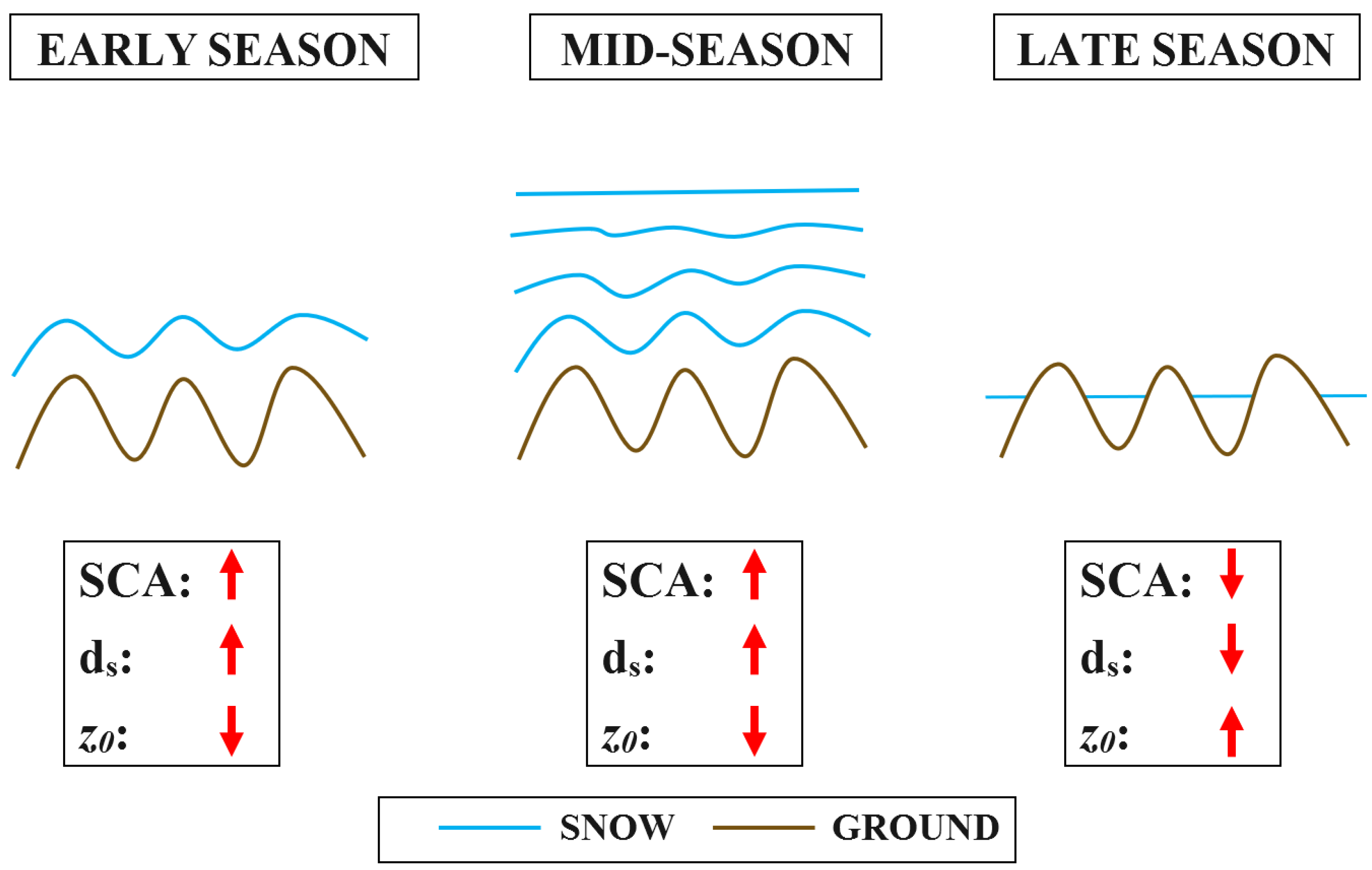
Figure 2.
Site locations around Northwest Colorado and the land cover type at each site.
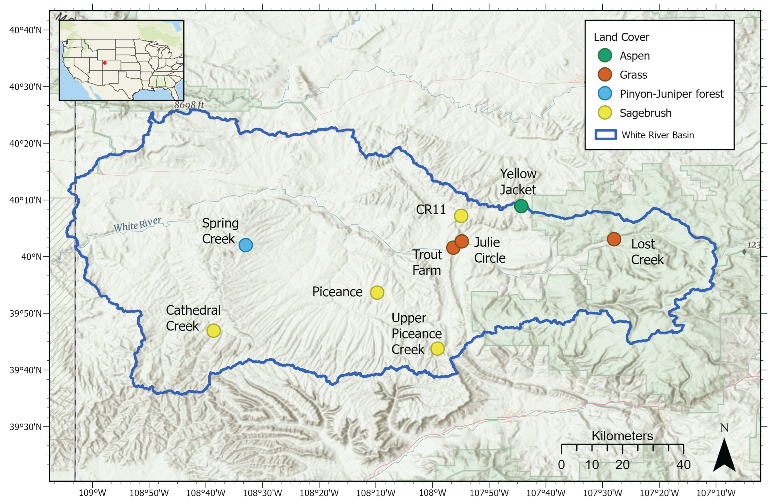
Figure 3.
Merged LiDAR scans shown in Cloud Compare from Julie Circle demonstrating and decoupling from underlying surface roughness features within the AOI. (a) a direct side profile view and (b) a top-side view. The bottom scan (snow free) was taken on 25 November 2019 and has a value of 0.4 x m. The middle scan is from 9 December 2019, with a depth of 0.21 m and of 4.2 x m. The top scan is from the highest of the season, at 0.52 m on 6 February 2020 with a of 35 x m.
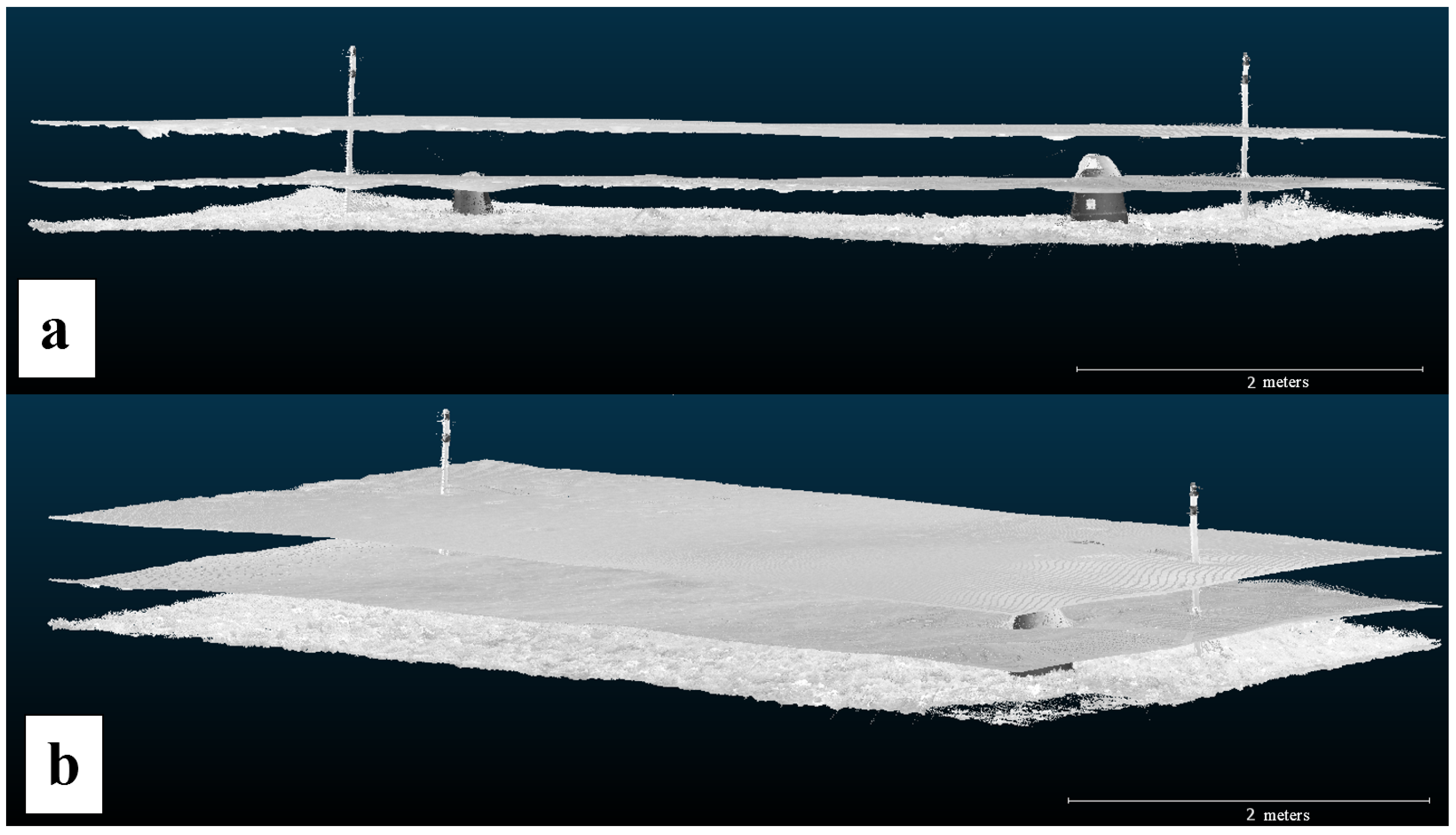
Figure 4.
Results of the study showing and ln() for (a) CR11, Julie Circle (JC), and Trout Farm (TF), (b) Cathedral Creek (CC), Piceance (P), Spring Creek (SC), and Upper Piceance Creek (UPC), (c) Lost Creek (LC), (d) Yellow Jacket (YJ). Details of the study sites are provided in Table 1 and Figure 2.
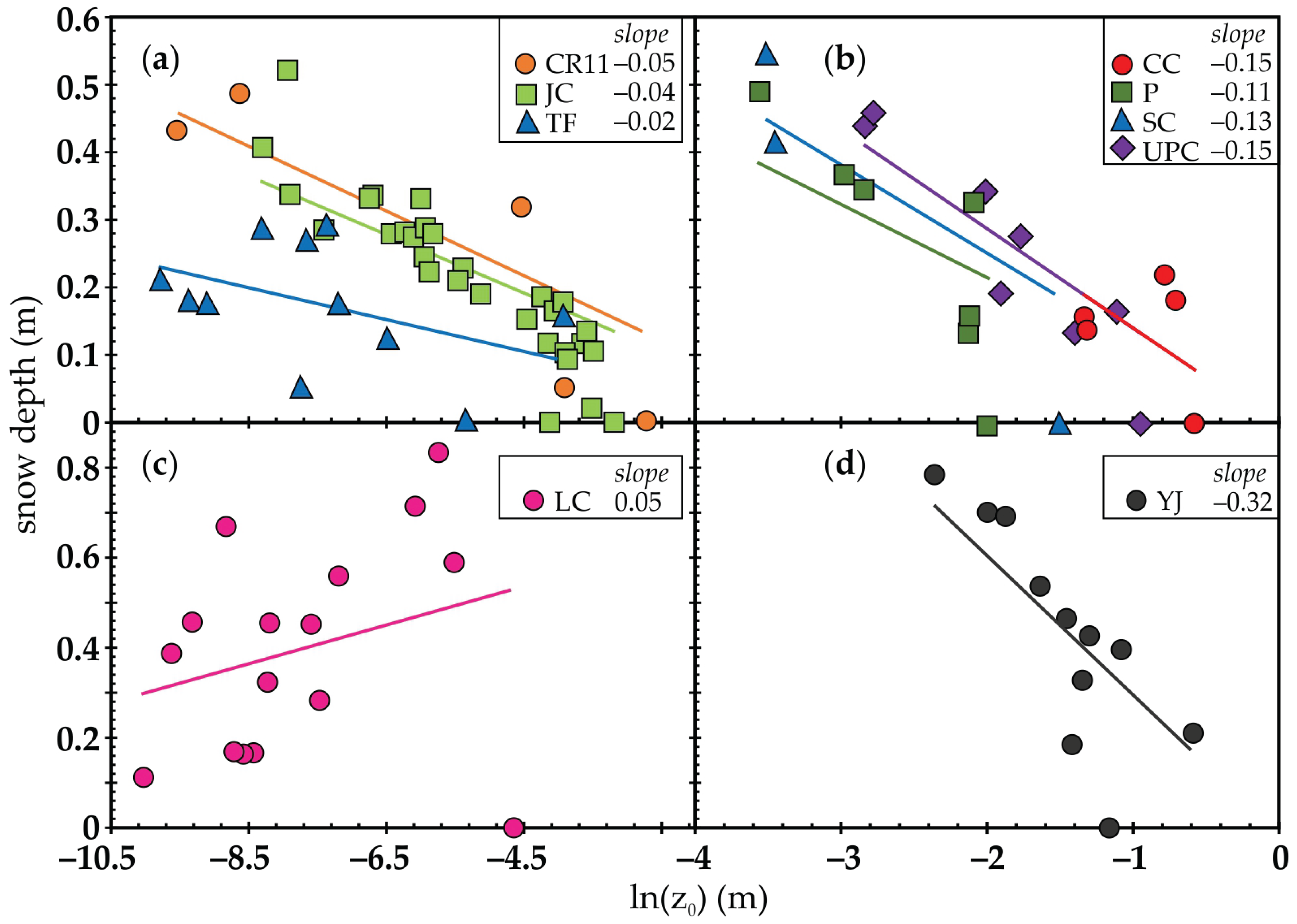
Figure 5.
Photos from the snow sites during snow cover. (a) Snowmobile tracks at Lost Creek on 26 February 2020, with a of 0.85 m and of 3.3 x m. (b) Site overview of Lost Creek with red arrow pointing to snowmobile tracks. (c) Trout Farm site looking south on 10 February 2020 ( of 0.29 m and of 0.63 x m) showing minor variations of the snow surface topography (red arrow). (d) Trout Farm on 25 February 2020 ( of 0.29 m and of 0.25 x m) showing a smoother snowpack surface. Note that the footprints included in the site are not within the AOI. (e) Yellow Jacket site taken on 16 March 2020 ( of 0.40 m and of 3.5 x m) recently after a snowmobile had driven through the site, plus the addition of sun cup development. (f) Yellow Jacket 7 April 2020 ( of 0.21 m and of 5.8 x m), site had extensive melt increasing the roughness.
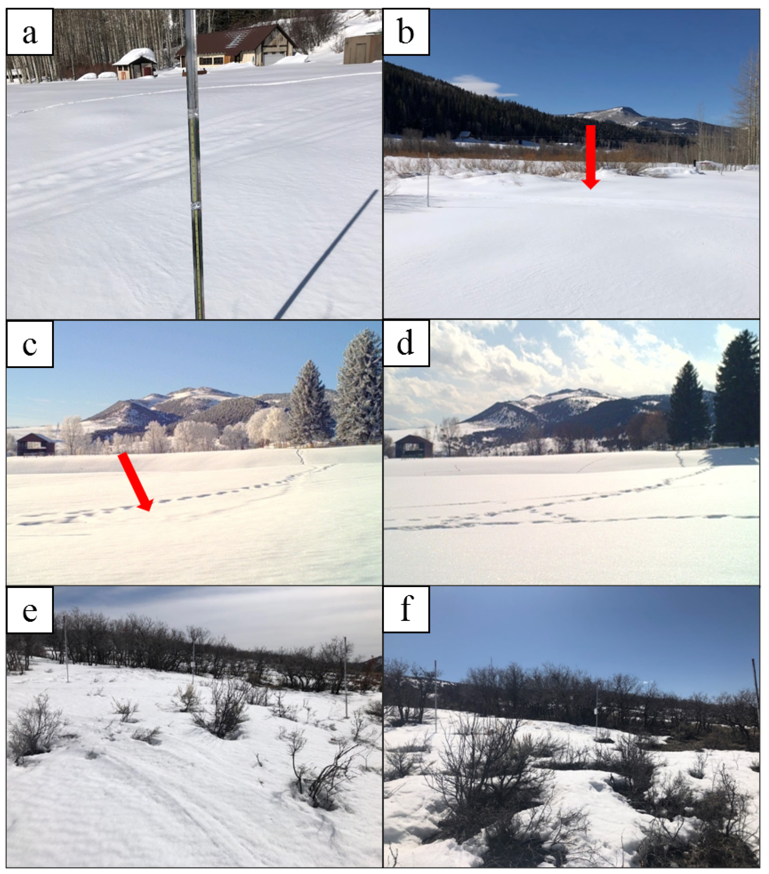
Figure 6.
Accumulation (blue) and melt (red) values from Julie Circle. Accumulation was defined as snow depth greater than the day before, and melt was defined as snow depth was than the day before.
Figure 6.
Accumulation (blue) and melt (red) values from Julie Circle. Accumulation was defined as snow depth greater than the day before, and melt was defined as snow depth was than the day before.
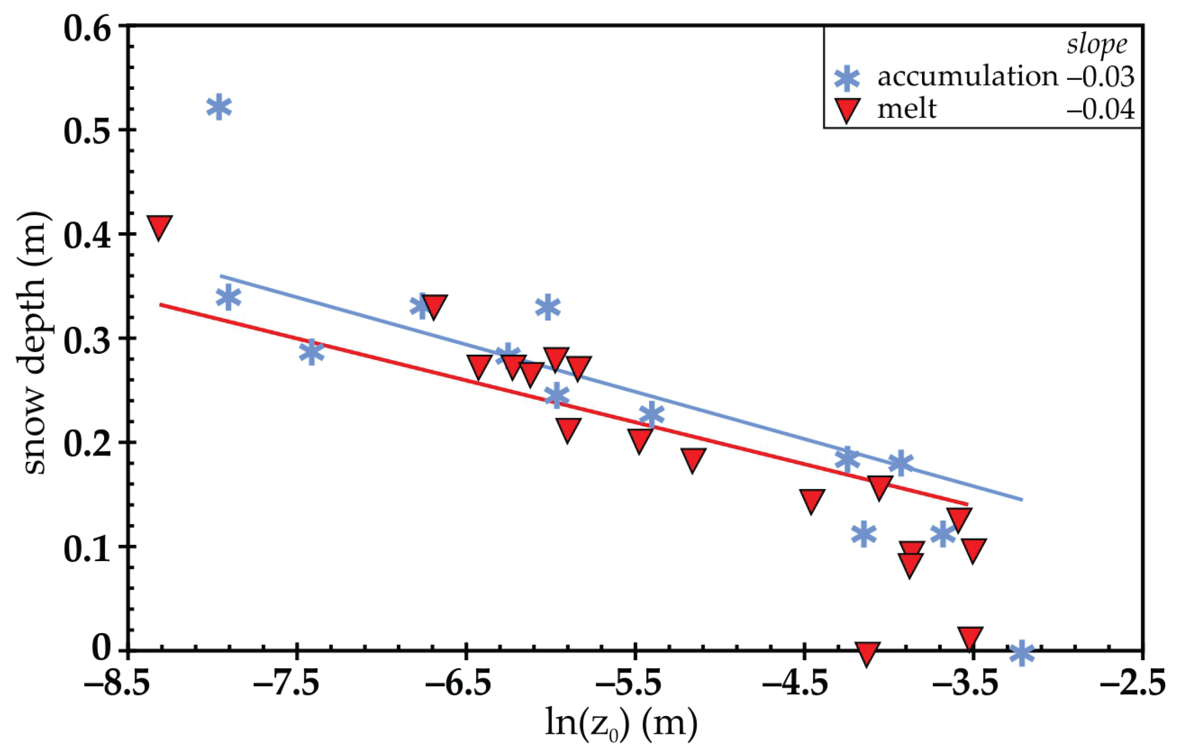
Figure 7.
Interpolated surfaces from the Cathedral Creek site on a) 16 January 2020 with a lower (0.15 m) and a lower value (2.7 x m), and b) 24 February 2020 with the highest recorded at the site (0.23 meters) and a very high value (4.5 x m. The red arrow highlights the larger surface features that are not large vegetation.
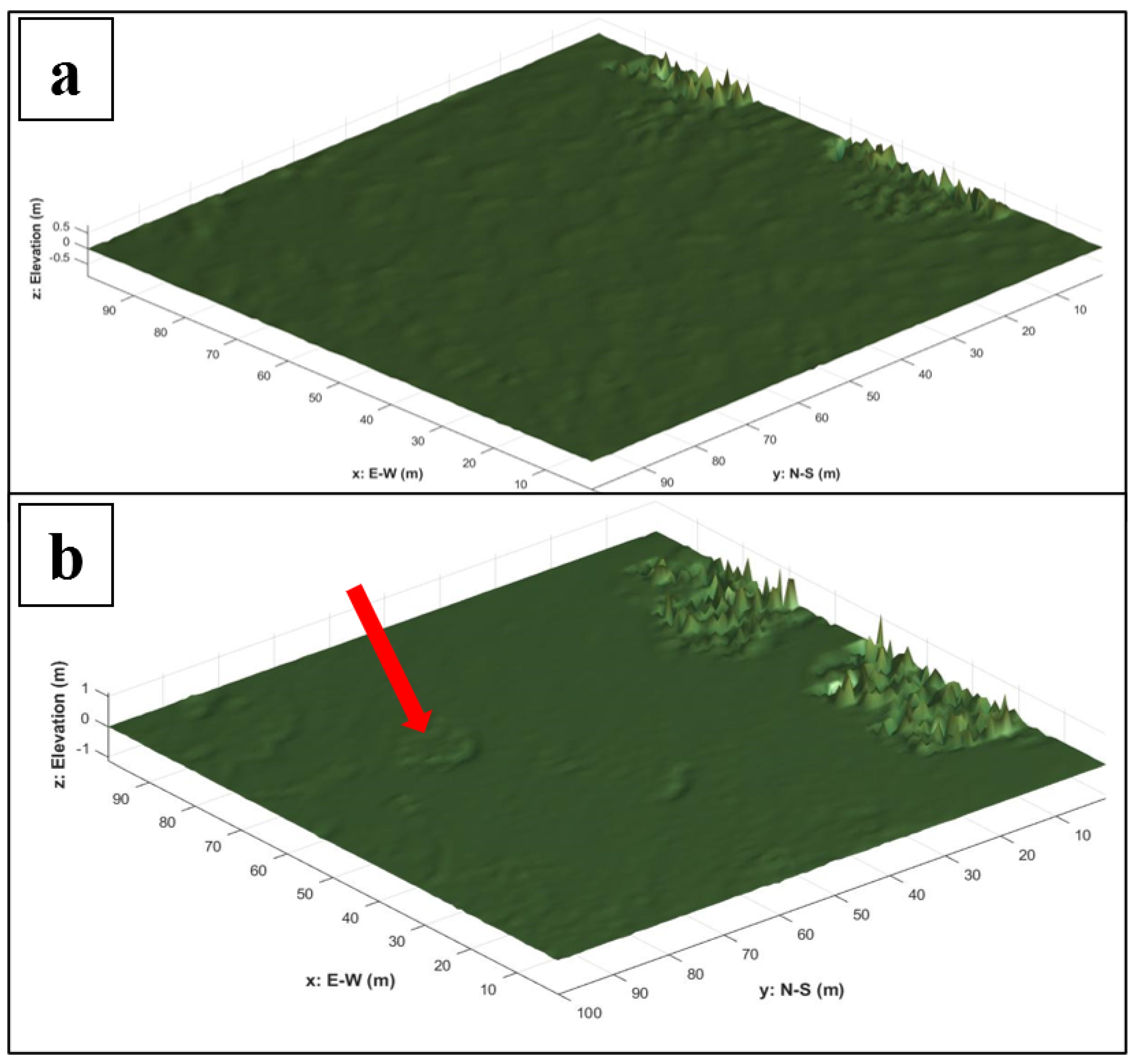

Table 1.
Description of the the nine study sites within the White River watershed of Colorado U.S. during the 2019-2020 winter season, including the average scan frequency, primary roughness feature height, and initial/snow-free .
Table 1.
Description of the the nine study sites within the White River watershed of Colorado U.S. during the 2019-2020 winter season, including the average scan frequency, primary roughness feature height, and initial/snow-free .
| Site Name | Scan Frequency | Primary Roughness Feature Height (m) | Initial (x m) |
|---|---|---|---|
| Trout Farm | Weekly | 0.01 | 5.0 |
| Cathedral Creek | Bi-weekly | 1.30 | 570 |
| Julie Circle | Every storm | 0.35 | 40 |
| CR11 | Bi-weekly | 0.46 | 66 |
| Upper Piceance | Bi-weekly | 1.65 | 390 |
| Yellow Jacket | Tri-weekly | 1.85 | 330 |
| Piceance | Bi-weekly | 0.68 | 110 |
| Lost Creek | Weekly | 0.13 | 9.0 |
| Spring Creek | Monthly | 1.10 | 220 |
Disclaimer/Publisher’s Note: The statements, opinions and data contained in all publications are solely those of the individual author(s) and contributor(s) and not of MDPI and/or the editor(s). MDPI and/or the editor(s) disclaim responsibility for any injury to people or property resulting from any ideas, methods, instructions or products referred to in the content. |
© 2025 by the authors. Licensee MDPI, Basel, Switzerland. This article is an open access article distributed under the terms and conditions of the Creative Commons Attribution (CC BY) license (http://creativecommons.org/licenses/by/4.0/).
Copyright: This open access article is published under a Creative Commons CC BY 4.0 license, which permit the free download, distribution, and reuse, provided that the author and preprint are cited in any reuse.


