Submitted:
24 September 2025
Posted:
24 September 2025
You are already at the latest version
Abstract
We introduced a possible electric charge forming mechanism, which includes the quasi normal mode calculations for a Kerr black hole with area of 4ln3 and spin 2 and the states generation by the preon model. We think the electric charge may exist as energy in the 3+1 space time with no need for additional dimension. And we think there might possibly be a tiny Kerr black hole net in our universe, which is sparse for electric charges and will select out the energies corresponding to electric charges as the only possible propagating wave energies. This net may at least be another possible way to have electric charge quantization except confinement, especially when we have to treat it as quantized energy propagating in the 3+1 space time. We also showed one more possibly interesting thing that electric charge may be the source of a Berry curvature to curve the 3+1 space time to form the conventional electromagnetic field.
Keywords:
quasi normal mode
; area triplet
; preon
; electric charge forming
; tiny Kerr black hole net
1. Introduction
Study on the perturbations of the gravitational field on astrophysical black holes has gained rich achievements [1,2,3]. Such as, the quantum properties of a Schwartzchild black hole have been related with their quasi normal modes [4], and its surface area is adjusted to have a discrete spectrum proportional to , rather than . The numerical analysis of quasi normal modes for rotating black holes has also been given by using the Teukolsky’s radial equation [5,6].
It then raised an interesting idea if we could apply the techniques on astrophysical black holes the same way as on those in the Planck scale. But first do black holes in Planck scale exist? Actually people have already studied quite a lot on these objects [7,8,9,10]. And then second could we perturb the Planck scale black holes the same way as those astrophysical black holes? It shall be asked since in the Planck scale we may have to deal with quantum gravity [11,12,13,14,15,16]. However, current quantum gravity theories have all encountered different troubles. We can not quantize gravity in a way similar as other fields. Gravity field is not a conformal field and is not renormalizable [17]. People tried to adopt the effective field theory on gravity [18], and recently there are quite a lot of interesting works based on this, such as checking the possibility of superposition of two masses and their entanglement [19,20,21,22]. But effective gravity field theory is at most a low energy quantum gravity theory, which excludes the study on Planck scale black hole. In the last decades, string theory has been given much expectation on helping to find a reasonable quantum gravity theory, but the extra dimensions and its caused problems make us hard to seriously accept it at this moment [23]. Loop quantum gravity tried to construct the quantized space time from beginning, but there are strong arguments on if it could have general relativity as its classical limits, and it is unlikely it described the real space time of our universe [24]. It seems the granulitization of space time is not a satisfying solution, and actually observations also do not support a granulized space time for our universe [25]. It is quite possible to have a classical gravity field outside a black hole even in the Planck scale, and we may still use the classical space time curvature tensor to describe the nature of gravity [14,15]. Furthermore, we may still adopt wave perturbation techniques, since it seems that they can tell us more about things that could not be described solely by the particle side.
Therefore in this paper we had tried to use the Teukolsky’s equation [26,27,28] on the black hole in Planck scale. We showed the quasi normal mode calculations for a Kerr black hole in Planck scale with an area of and spin angular momentum of [29]. In part 2.1, we introduced the techniques to calculate the quasi normal modes of this Planck scale black hole, and then in part 2.2 we will show our finding that the numerical calculations for this Planck scale black hole can give a value that can be related to e/3. In section 2.3, we will further show that the electric charge of leptons and quarks can be naturally formed out by further introducing the preon model after we get e/3. Necessary discussions are made in section 3. Conclusions are drawn in section 4.
2. Calculation Model and Possible Electric Charge Forming Mechanism
In this section, we will introduce the calculations for the quasi normal modes of a Kerr black hole in Planck scale with an area of and spin angular momentum of . And the possible electric charge forming mechanism is then explained.
2.1. Model
A realistic model of wave dynamics in black-hole space times involving a non-spherical background geometry with angular momentum has already been provided. In terms of the Boyer-Lindquist coordinates, the space time of a rotating Kerr black hole is described by the line element:
where , , M is the mass, and a is the angular momentum per unit mass of the black hole, respectively. (Here the gravitational units G=c=ħ=1 are used).
The perturbations of rotating relativistic objects was first studied by Teukolsky by making use of the famous Teukolsky master equation [26,27,28]. It describes the perturbations Ψ(t, r, θ, ϕ) of all physically interesting spin-weights s to the Kerr background metric in terms of the corresponding Newman–Penrose scalars [26]. The quasi-normal modes of the Kerr black holes can then be obtained by proper boundary conditions for the Teukolsky master equation. A first numerical study of Kerr Quasi normal modes was made by Detweiler [30,31]. And various significant results can be found in a lot of references [32,33,34].
In the Kerr case, due to the non-spherical symmetry of the background, the perturbation problem does not reduce to a single ordinary differential equation for the radial part of the perturbations like in the Schwarzchild case, but rather to a system of differential equations with one equation for the angular part of the perturbations, and a second equation for the radial part, while these two are in principal coupled together, which means we have to solve two differential equations simultaneously together. This increases the difficulties, but after years of working by physicists in the field, it can be done as the following [5,6,35]. Just as we talked above, by assuming the wave function as:
where are Boyer-Lindquist coordinates. This then gives a radial and an angular equation coupled by a separation constant , where
The spin-weight parameter s specifies the equation to gravitational (s=2), electromagnetic (s= 1), scalar(s=0), or two-component neutrino (s=1/2) fields as said above.
An analytical solution can then be found that the real part of the Kerr black hole’s quasi normal mode can then be written as , with , , [5].
To get these analytical parameters is in general quite time consuming, and an rather simplified analytical solution of the above parameters using elliptical functions can be found in reference [6].
The energy of these quasi normal modes is then compared with what we can extract from the black hole’s ergosphere by the Penrose process. For Penrose process, we know the irreducible mass can be written as:
And therefore the energy that can be extracted is:
2.2. Calculations to Get e/3
Numerical calculation are made just like in references [5,6,35]. In Figure 1, the real part of the quasi normal mode frequency multiplied by mass versus the angular momentum to mass ratio is plotted. The line fits well with the numerical calculations in reference [5,6,35], except that we chose m = −2 [36,37], rather than m=-1 in the plot.
However, what we are interested right now is to see what will happen for a Kerr black hole in the Planck scale. Therefore, we chose the point as shown as a cross in the plot. For this point, it has area equal to and spin angular momentum equals to . Therefore the total mass would be:
And the angular momentum to mass ratio is:
From equation 11, we can find that the minimum mass of the Kerr black hole is 4.1527 Planck mass. At this point in the figure, the real part of the quasi normal mode frequency gives an energy of 5.5901e7J, which corresponds to a mass of 6.2195e-10kg. What is really interesting is that, using the equation of , this finally gives the value of , where e is the measured electric charge unit. The value of we calculated here is about 3.3520‰() larger than the measured value.
and have the same dimension, and by setting the quantity of equal to that of . However, here we want to stress that it would be better to go directly as:
For this minimum Kerr black hole in the Planck scale, we then studied the Penrose process, i.e., the maximum amount of energy can be extracted from this minimum Kerr black hole. From equations 9-10, it is found that this energy is 2.2939e-10 kg, much less than the energy of quasi normal mode that corresponds to e/3. Since the maximum energy that can be extracted from this minimum Kerr black hole is much less than the quasi normal mode with the energy corresponding to e/3, therefore, for this minimum Kerr black hole, when it is perturbed, at the beginning, it cannot extract energy from it. Rather, it will absorb positive energy or extract no energy. However, it may not grow too, for it may not keep more energy for there are mechanisms such as Hawking radiation. It is more possible these tiny Kerr black holes are stable quanta. It is necessary to mention that the Penrose process may be not able to describe the physics here exactly, but we still think that it could at least be used to do the evaluation.
2.3. The Preon Model
The preon model was first proposed by Pati and Salam in 1974 [38]. They put a name of preon for their hypothetical constituent particles, and this was then gradually adopted to refer to the sub-quark/sub-lepton particles of various models. There are actually several kinds of preon models developed, see for example [39,40,41,42], including an interesting proposal of the so-called Rishon model by Harari and Shupe simultaneously [43,44]. In Harari’s model, it involves just two kinds of ‘rishons’, one carrying an electric charge of +e/3 where −e is the charge on the electron, the other neutral. Particles in the standard model may be formed like this: the rishons combine into triplets, with the two “three-of-a-kind” triplets being interpreted as the and e+, and the permutations of triplets with an “odd-man-out” being interpreted as the different colors of quarks. The above proposals of the preon model solves some problems, but unfortunately, it also caused a lot of problems, including the lack of a dynamical framework, and the lack of an explanation as to why there are only two kinds of rishons [43,44] or three kinds of Helons [45] and where the triplets comes from [46,47]. Here we will introduce our better way to make the preon theory more complete and reasonable, and will show that, by noticing that there is one more quantum number describing the degenerated area triplet of the Kerr black hole in the Planck scale, the preon model could use the two numbers, that is, the magnetic momentum quantum number and the area triplet number, to get the electric charges for quarks and leptons.
We know for this black hole, it has the area triplet degenerate states, and here we have the choices of m=0, +2, -2. If we define two numbers of ka, and km, corresponding to area triplet state and angular momentum of this Kerr black hole in the Planck scale, then if the total extract energy from this Kerr black hole is zero, then we can have –e with one state, 0 with one state, -e/3 with three states, and +2e/3 with three states as positive matter, or we can have +e with one state, 0 with one state, +e/3 with three states, and -2e/3 with three states as negative matter. Adding these states together equals zero, which means we could extract zero energy from the Kerr black hole. And this makes 8 states, which just makes the standard model particles. It is necessary to mention that, like such as in references [43,44,45], we did not allow the mixing of km=2 and km=-2, and here we could just get the same results, but with a more reasonable basis.
To be more specific on how the 8 states are formed, we list the process of positive matter generation as in Table 1. The form of the 8 states may be like: the first one is the three degenerate states of ka all have km=+2, and the quasi normal mode forms lepton with electric charge -e; the second one is the three degenerate states of ka all have km=0, and the quasi normal mode corresponds to lepton with zero electric charge; the third one is one of the degenerate three states of ka have km=+2, which forms the quark with electric charge –e/3; and the fourth one is two of the three degenerate states of ka has km=-2, which forms the quark with electric charge +2e/3. The third one and the fourth one can have three colors each. All eight states give zero energy.
3. Discussion
It is currently still an open question what is an electric charge and how to get it in a reasonable way. Electric charge is generally associated with the U(1) gauge field. Or as shown in Dirac quantization, it is related with magnetic monopole charge. And in string theory, electric charge can be found by having non-zero momentum in one compact direction. However, the phenomenon of electric charge quantization and especially why the electric charge has the measured value like that remains like an enigma. We can see that electric charge is a property which is currently put into the standard model theory by hand.
Therefore we think it would be intriguing to give a possible mechanism as shown in this paper. Especially this mechanism gives an electric charge value which is so close to the measured one. You may say that for this value there is still a derivation of 3.3520‰, and we think this may be due to that the Teukolsky master equation is of the first order approximation. But this value of the electric charge in such accuracy is really what we can get at the first time, which should be exciting, and it would be natural if we want to extrapolate more and deeper possible physics by further examining the mechanism and its background conditions.
From equation 13, it seems to indicate that the electric charge may be a kind of energy. This is not something new, which has actually been widely adopted in sting theory, or could be traced back to Kaluza and Klein’s work [48,49], where the electric charge could be found by having quantized momentum in one compact dimension. And actually the form of equation 13 was also proposed out by Kaluza in his original paper [48]. Quantization of momentum in one compact dimension may mean there are excited states too, which may mean it can have electric charge with quantum number larger than one. And for string theory, it also predicted that string may have many kinds of fractal electric charges, but which could not be found in lab yet. We are not trying to be picky on string theory here, and we intend to think that string theory is still in its early developing stage. But it does not seem that additional dimensional confinement is the case from our mechanism, and it is more possible that the electric charge is in the 3+1 space time.
There is another problem to take electric charge as quantized energy in a confined dimension, which is that how this additional dimension could be curved to have this length exactly. However, if as we said the electric charges are energies in the 3+1 space time, it would have to face other problems too, such as how could they keep having the quantized energies, especially there could be a whole lot of possible interactions on their way with other particles in the 3+1 space time, and it would be strange if there are no interactions for them to shift their energies.
One possible way to solve this might be that we think there might be a tiny Kerr black hole net in the universe, and the way electric charge exists in this 3+1 space time may be also like a coupling effect by which the fermion mass is formed. For fermion mass, it is formed by its field coupled with vacuum, or a scalar field, while for electric charge, in a similar way, we think it is also likely formed by waves coupled with this tiny Kerr black hole net. This coupling makes the energies corresponding to electric charge the only allowed characteristic wave energies in this 3+1 space time. So like vacuum, we think there may be a Kerr black hole net in the Planck scale in this universe. The picture of a net can also be found somewhere else such as in loop quantum gravity, which somehow is borrowed to this place, but sure physically these two nets are really different.
The energy states of electric charges can be newly generated out anywhere at present in the universe, such as in the case of the electron positron pair generation, which thus excludes the possibility that they are only the remnant states generated from the Planck scale Kerr black holes of early time universe, and provide another supporting for the existence of a widely spread net in the present universe to do the energy states selection. It shall note that Dirac gives a way to explain the electron positron pair generation by the picture of a filled up energy band. This band is filled up with pre-formed electrons, and therefore there may be no need for these electrons to be generated at current time. The concept of band structure may be useful for solids, but it is not clear how this band could be formed for the universe. And if there is a band, it will need huge amount of pre-formed electron states to be or to fill up the background in the universe, which may be a problem. These make the energy band not a good choice for the universe as for the solids. Also in that picture it did not tell us how these electron states filling the energy band could be formed at the beginning. Therefore we adopted that the generation of particle antiparticle pairs could be from this energy states selection net, rather than from a pre-formed band.
As in earlier discussions, the tiny Kerr black holes in the Planck scale may be formed as big black hole evaporation remnants, or as the remnants of early universe with extremely high temperature. But if we think there is a net of tiny Kerr black holes, maybe we need to further consider some additional forming process, since they are widely distributed and it is possible their numbers may also grow with the universe. It is not clear what exactly this process could be and how this tiny Kerr black hole net is distributed in detail at this moment, which may need further work, but we think the existence of this tiny Kerr black hole net is really not unconceivable, and it may be sparse for electric charges and its resulting effect is to have energies corresponding the electric charges as the only characteristic propagating wave energies. We think the quantum fluctuation, and the area quantization process may be important to form this net. And the distribution of this tiny Kerr black hole net may tell us a lot more information about the background of our universe. Anyway, if this net does exist, it may indicate that there are plenty of physics unaware by us to explore in the high energy part, i.e. the Planck scale or even beyond. It is certain we are in the low energy part, or at least our lab results can not directly reach the Planck scale right now. However, they can be noticed when there are couplings between the high energy part and the low energy part. Such as, we think the electric charge of fermions could be detected after the spin 1/2 field is further coupled with the vacuum to have mass. Therefore it may also have promising detectable discoveries based on these couplings. Also we shall think about the way how it could fit the current knowledge on our universe. We find the idea of a mother universe might be attractive here [50].
We shall note that our calculations are based on that the space time is not quantized. Having quanta of Planck scale Kerr black holes may not mean the space time is granulized too. Anyway, it is noticed that current observations also seem do not support a granulized space time. And we found the quanta of these tiny Kerr black holes could not be found by quantization of the gravity field in a normal way. At least the area quantization of black holes could only be realized by the quasi normal mode calculations, which is a wave perturbation method. A mathematical consistent way for gravity field quantization is not yet touchable at this moment or is at least controversial. The way of field canonical quantization may not be able to tell all the things only by itself, especially for the Planck scale Kerr black holes, and it needs wave perturbation method.
One more maybe interesting thing is that you can form the classical electromagnetic equations in a way similar to the equation of general relativity, if we think both are the results of curvature sourced by the energy and momentum in 3+1 space time. We can show this here below. And here we adopt Berry curvature for electric charge, rather than Ricci curvature for mass. Berry curvature is generally for Hilbert space, and it has been borrowed to describe 3+1 space time here.
By splitting the equation of , Dirac got for electrons. It may be good if we write down:
to deal with electrons’ effect on the space time, corresponding to for masses. is a vector, corresponding to , which is a tensor. , and is the effect of electric charge on background space time, which is small. Therefore, we have:
Just like the covariant derivation of is zero, we also make the covariant derivation of zero. Therefore we have:
, and keep only the zeroth term for , then we have , and:
Here we assumed that the derivative of one coordinate basis will not be affected by the other three, which is reasonable for small .
Then we have the Berry curvature:
Contraction of and gives:
Using the Lorentz gauge and making the electric charges and their movement in the 3+1 space time as the source terms of energy momentum vector, we then get the usual electromagnetic field equation. By these treatments, we show that the electromagnetic field could be found by curving the 3 + 1 space time described by a vector in the 3+1 space time with no need for additional dimension. This meets our thought that electric charges could be the energies in the 3+1 space time, and they could be the sources to curve the 3+1 space time to give the normal electromagnetic field equations. These calculations might be interesting.
4. Conclusions
In this paper, we introduced a possible electric charge forming mechanism. The quasi normal mode calculations for a Kerr black hole with area of and spin 2 give an energy corresponding to e/3. Together with the area triplet, the preon model can form electric charges for all the fermions. There might possibly be a tiny Kerr black hole net as the background for our universe, which is sparse for electric charges and its resulting effect is to select out the energies corresponding to electric charges as the only possible propagating wave energies in our universe. Anyway, we think the existence of this net is really not unconceivable and may seem to be a better way to give quantized electric charge than the confinement effect from an additional dimension, or at least it theoretically provides another possible way at this moment. Our work is not based on a granulized space time, and we think the wave perturbation method may be indispensable here. At last, we also tried to show one more possibly interesting thing that the conventional electromagnetic field equation could be found out by curving the 3+1 space time sourced by the energy momentum vector from electric charge. The concept of Berry curvature rather than Ricci curvature is adopted here.
Funding
This research received no external funding.
Conflicts of Interest
The author declares no conflicts of interest.
References
- X. Cai; and Y. Miao. Phys. Rev. D 2020, 101, 104023.
- Malybayev, K. Boshkayev; V. Ivashchuk, Eur. Phys. J. C 2021, 81, 475.
- R. Konoplya, Rev. Mod. Phys. 2011, 83, 793.
- S. Hod, Phys. Rev. Lett. 1998, 81, 4293.
- U. Keshet; S. Hod, Phys. Rev. D 2007, 76, R061501.
- H. Kao; and D. Tomino, Phys. Rev. D 2008, 77, 127503.
- Y. Aharono; A. Cashe; and S. Nussinov, Phys. Letts. B 1987, 191, 51.
- L. Susskind, 1995. <arXiv: hep-th/9501106>.
- Ashtekar; M. Bojowald, Class. Quant. Grav. 2005, 22, 3349.
- G. Domenech; M. Sasaki, Class. Quant. Grav. 2023, 40, 177001.
- K. Eppley; E. Hannah, Found. Phys. 1977, 7, 51.
- D. Page; C. Geilker, Phys. Rev. Lett. 1981, 47, 979.
- P. Pearle; and E. Squires, Found. Phys. 1996, 26, 291.
- MØller, Les theories relativistes de la gravitation (CNRS, Paris, 1962).
- L. Rosenfeld, Nucl. Phys. 1963, 40, 353.
- S. Carlip, Rep., Prog. Phys. 2001, 64, 885.
- Shomer, 2007, <arXiv: hep-th/0709.3555>.
- J.F. Donoghue, Quantum General Relativity and Effective Field Theory. In: Bambi, C., Modesto, L., Shapiro, I. (eds) Handbook of Quantum Gravity. Springer, Singapore, 2024.
- Belenchia; R. Wald; F. Giacomini; E. Castro-Ruiz; Č. Brukner; M. Aspelmeyer, Phys. Rev. D 2018, 98, 126009.
- Danielson; G. Satishchandran; R. Wald, Phys. Rev. D 2022, 105, 086001.
- J. Wilson-Gerow; Y. Chen; P. Stamp, Phys. Rev. D 2024, 109, 064078.
- Y. Liu; H. Miao; Y. Chen; Y. Ma, Phys. Rev. D 2023, 107, 024004.
- J. de Boer, Nucl. Phys. B – Proc. Suppl. 2003, 117, 353.
- A Perez, 2004, <arXiv:gr-qc/0409061>.
- Z. Cao et.al., Phys Rev. Letts. 2024, 133, 071501.
- S. Teukolsky, Astrophys. J. 1973, 185, 635.
- Leaver, J. Math. Phys. 1986, 27, 1238.
- J. Hartle; D. Wilkins, Comm. in Math. Phys. 1974, 38, 47.
- T. Xia, Mod. Phys. 2023, 13, 1.
- S. Detweiler, Astrophys. J. 1978, 225, 687.
- S. Detweiler; J. Ipser, Astrophys. J. 1973, 185, 685.
- H. Yang; A. Zimmerman; A. Zenginoglu; F. Zhang; E. Berti; Y. Chen, Phys. Rev. D 2013, 88, 044047.
- Berti; V. Cardoso; K. Kokkotas; H. Onozawa, Phys. Rev. D 2003, 68, 124018.
- P. Pani; E. Berti; L. Gualtieri, Phys. Rev. D 2013, 88, 064048.
- Berti; V. Cardoso; S. Yoshida, Phys. Rev. D 2004, 69, 124018.
- L. Motl, Adv. Theor. Math. Phys. 2003, 6, 1135.
- L. Motl; A. Neitzke, Adv. Theor. Math. Phys. 2003, 7, 307.
- J. C. Pati; A. Salam, Phys. Rev. D 1974, 10, 275.
- Terazawa; K. Akama, Phys. Lett. B 1980, 97, 81.
- K. Akama; I. Oda, Physics Letters B 1991, 259, 431.
- S. Dimopolous; S. Raby; L. Susskind, Nucl. Phys. B 1980, 173, 208.
- K. Babu; J. Pati, Phys. Rev. D 1993, 48, R1921.
- Harari, Phys. Lett. B 1979, 86, 83.
- M. Shup, Phys. Lett. B 1979, 86, 87.
- S. B. Thompson, available from: <arXiv:hep-ph/0503213>.
- P. Żenczykowski, Phys. Lett. B 2008, 660, 567.
- F. Sandin; J. Hansson, Phys. Rev D 2007, 76, 125006.
- T. Kaluza, Sitzungsber. Preuss. Akad. Wiss. Berlin (Math. Phys.) 1921, 966, <arXiv.org/abs/1803.08616>.
- Klein, Zeitschrift fÜr Physik 1926, 37, 895.
- L. Shamir, MNRAS 2023, 538, 76.
Figure 1.
The real part of the quasi normal mode frequency. The cross point has the area of and J = 2. M = −2, rather than m=-1, is chosen.
Figure 1.
The real part of the quasi normal mode frequency. The cross point has the area of and J = 2. M = −2, rather than m=-1, is chosen.
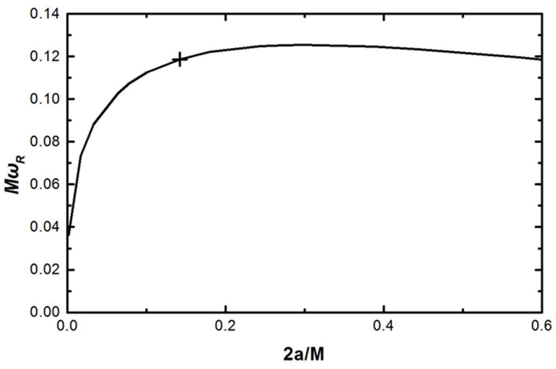

Table 1.
The charges of leptons and quarks are formed from two numbers of ka and km. ka1, ka2, and ka3 are three degenerate states, which come from area triplet.
Table 1.
The charges of leptons and quarks are formed from two numbers of ka and km. ka1, ka2, and ka3 are three degenerate states, which come from area triplet.
| charge | ka1 | ka2 | ka3 | colors | Type |
|---|---|---|---|---|---|
| -e | +2 | +2 | +2 | 1 | lepton |
| 0 | 0 | 0 | 0 | 1 | |
| -e/3 | +2 | 0 | 0 | 3 | quark |
| 0 | +2 | 0 | |||
| 0 | 0 | +2 | |||
| +2e/3 | 0 | -2 | -2 | 3 | |
| -2 | 0 | -2 | |||
| -2 | -2 | 0 |
Disclaimer/Publisher’s Note: The statements, opinions and data contained in all publications are solely those of the individual author(s) and contributor(s) and not of MDPI and/or the editor(s). MDPI and/or the editor(s) disclaim responsibility for any injury to people or property resulting from any ideas, methods, instructions or products referred to in the content. |
© 2025 by the author. Licensee MDPI, Basel, Switzerland. This article is an open access article distributed under the terms and conditions of the Creative Commons Attribution (CC BY) license (http://creativecommons.org/licenses/by/4.0/).
Copyright: This open access article is published under a Creative Commons CC BY 4.0 license, which permit the free download, distribution, and reuse, provided that the author and preprint are cited in any reuse.


