
Submitted:
23 September 2025
Posted:
24 September 2025
You are already at the latest version
Abstract
The diffusion probability model is a state-of-the-art generative model that generates an image by applying a neural network iteratively. Moreover, this generation process is regarded as an algorithm solving a diffusion ordinary differential equation (ODE) or stochastic differential equation (SDE). Based on the analysis of the truncation error of the diffusion ODE and SDE, our study proposes a training-free algorithm that generates high-quality 512 x 512 and 1024 x 1024 images in eight steps, with flexible guidance scales. To the best of my knowledge, our algorithm is the first one that samples a 1024 x 1024 resolution image in 8 steps with an FID performance comparable to that of the latest distillation model, but without additional training. Meanwhile, our algorithm can also generate a 512 x 512 image in 8 steps, and its FID performance is better than the inference result using state-of-the-art ODE solver DMP++ 2m in 20 steps. The result of our algorithm in generating high-quality 512 x 512 images and 1024 x 1024 images with five-step and six-step inference is also comparable to the latest distillation model. Moreover, unlike most distillation algorithms, which achieve state-of-the-art FID performance by fixing the sampling guidance scale, and which sometimes cannot improve their performance by adding inference steps, our algorithm uses a flexible guidance scale on classifier-free guidance sampling. The increase in inference steps enhances its FID performance. Additionally, the algorithm can be considered a plug-in component compatible with most ODE solvers and latent diffusion models. Extensive experiments are performed using the COCO 2014, COCO 2017, and the LAION dataset. Specifically, we validate our eight-step image generation algorithm using the COCO 2014, COCO 2017, and LAION validation datasets with a 5.5 guidance scale and a 7.5 guidance scale, respectively. Furthermore, the FID performance of the image synthesis in 512 x 512 resolution with a 5.5 guidance scale is 15.7, 22.35, and 17.52, meaning it is comparable with the state-of-the-art ODE solver DPM++ in 20 steps, whose best FID performance is 17.3, 23.75, and 17.33, respectively. Further, it also outperforms the state-of-the-art AMED-plugin solver, whose FID performance is 19.07, 25.50, and 18.06. We also apply the algorithm in five-step inference without additional training, for which the best FID performance of our algorithm in COCO 2014, COCO 2017, and LAION is 19.18, 23.24, and 19.61, respectively, which is comparable to the performance of the state-of-the-art AMED Pulgin solver in eight steps, SDXL-turbo in four steps, and the state-of-the-art diffusion distillation model Flash Diffusion in five steps. Then, we validate our algorithm in synthesizing 1024 * 1024 images, whose FID performance in COCO 2014, COCO 2017, and LAION using eight-step inference is 17.84, 24.42, and 19.25, respectively. Thus, it outperforms the SDXL-lightning in eight steps, Flash DiffusionXL in eight steps, and DMD2 in four steps. Moreover, the FID performance of the six-step inference of our algorithm in the 1024 x 1024 image synthesis is 23, which only has a limited distance to the state-of-the-art distillation model mentioned above. We also use information theory to explain the advantage of our algorithm and why it achieves a strong FID performance.
Keywords:
computer vision
; artificial intelligent generative content
; diffusion ODE solver
; diffusion model
1. Introduction
The diffusion probability model (DM)[1], a state-of-the-art image generation model with solid mathematics instruction on image sampling, is among the most popular research areas in computer vision. A typical diffusion model, such as stable diffusion (SD)[2], is inspired by the Brownian diffusion process in physics. It consists of two different processes: diffusion and reverse. The diffusion process adds small variants of Gaussian noise to the image step by step to facilitate its gradual conversion into pure Gaussian noise, while the reverse process uses the score matching[3] algorithm to train a neural network studying the gradient of the diffusion process by denoising noisy images[4]. Then, the reverse of the diffusion process occurs. The diffusion process can be described by a diffusion stochastic differential equation (SDE) whose form is similar to the Brownian diffusion SDE. Moreover, the reverse process can be described by an ordinary differential equation (ODE) or an SDE[3]. The ODE is equivalent to the SDE in the reverse process, which generates random variables step by step by transporting the standard Gaussian distribution to a target probability distribution by changing its geometric shape. However, it requires fewer inference steps to sample a high-quality image than solving the SDE, as it prevents involving a random effect during sampling. However, solving diffusion ODEs still requires a large amount of computational resources. Hence, solving this problem remains an active research area. Research related to it can be categorized into two classes. The first class proposes a training-free algorithm aimed at providing a good SDE and ODE solver tailored to the diffusion process[1,5,6,7,8,9]. The second class deems the whole inference process, which uses a neural network iteratively, as a large neural network, and it reduces the inference steps by training a small distillation model[10,11,12,13,14,15,16,17,18,19]. The training-free method typically necessitates a 20-step inference[5], while algorithms requiring additional training can generate an image within four to eight steps. However, our results show that by selecting the proper hyperparameter of the ODE solver and adding a training free diffusion model decorator to exploit the capability of the latent diffusion model, the inference speed can exceed expectations. To that end, we propose a new inference method that can generate 512 x 512 images in eight steps without additional training, and its Frechet Inception Distance (FID)[20] performance surpasses that of the state-of-the-art ODE solver in 20 steps. Furthermore, when applying our algorithm in the five-step inference, it also outperforms the state-of-the-art distillation algorithm in the same number of steps. We also apply our algorithm to 1024 x 1024 image generation, and the FID performance of the eight-step inference exceeds most of the latest distillation models in eight steps. We perform extensive experiments using the COCO 2014[21], COCO 2017 [21], and LAION datasets[22], and exhibit the generation result in Figure 1. We also use information theory to explain why our algorithm achieves a strong FID result.
2. Related Work
2.1. Diffusion ODE
The image generation process that uses a diffusion model can be regarded as solving a special diffusion SDE or ODE. A typical diffusion model has two processes: forward and reverse. The forward process perturbs the image by adding Gaussian noise to it, which can be described by the following SDE:
where the w is a standard Wiener process. Choosing different and corresponds to applying different algorithms. In this study, we use the variant preserve (VP) SDE[3] to describe the diffusion process, which corresponds to the denoised diffusion probability model (DDPM) algorithm[23]. Specifically, its choice is as follows:
By solving the Equation (1) step by step with a given , we obtain a noisy image . Finally, when applying iteration in T step, we obtain . Additionally, using the reparameterization algorithm, we can sample within one step[1].
In contrast, the reverse process, which corresponds to generating an image from a pure Gaussian noise, can be described by the following time-dependent ODE[8]:
where c is the condition of input, like the caption that describes the image, , where . Moreover, the score function normally used in VP SDE, it is trained by Equation (6)
and is the probability distribution of the random variables sampled by adding noise to the training images in timestep t.
Specifically, the and is defined by Equation (7) and Equation (8):
where .
Using Equation (5) as a reverse ODE can help exploit the advantage of adapting the DDPM algorithm to the common diffusion framework proposed by Karras [8]. However, the algorithm implementation should also consider whether a neural network can study this input–output pair if the input and output in different timesteps have an obvious gap in the variance when using this framework. So, to let the neural network study properly, we should formulate the equation as
where is the real function that the neural network studies, scales the input to reduce its variance, scales the output to use the common framework proposed by Karras, and transforms the variance to the condition input t of the neural network.
For simplicity, the following section will use to denote the centrifuge of the possible denoised images predicted by the neural network when given a noisy image :
where in DDPM.
2.2. Diffusion ODE Solver
Sampling an image from a diffusion model is equivalent to solving the Equation (5). Moreover, different solvers have been considered in previous research[5,8,24]. The inference process approximates the trajectory of the reverse ODE by discretizing its path. The research on reverse ODE solvers attempts to precisely estimate the next step, thereby minimizing the truncation error caused by the discretization. As the culmination of the truncation error will affect the result of synthesis, minimizing the truncation error in each step is equivalent to subtracting the demand for an increased inference step that has caused precise discretization.
Among those solvers, the DPM++ solver[5] is the latest state-of-the-art solver designed specifically for classifier-free guidance (CFG)[25] sampling. It predicts the next step via the following formula:
where is a log signal-to-noise ratio (SNR) of the noisy image, while the function transforms to the corresponding t.
We use the Taylor formula to obtain an approximation of the Equation (11), and then there is a first-order DPM++1s solver:
in which .
Moreover, by using a multistep method, we obtain the second-order DPM++2m solver:
where is as follows:
and .
2.3. Diffusion Distillation
The training-free method, which optimizes the truncation error in each step to minimize the demand for precise discretion. Unlike this method, the distillation algorithm[10,11,12,15,16] considers the whole inference process of applying a neural network iteratively as a large neural network. The distillation algorithm, which normally trains a small neural network, entails reducing its inference steps. However, training a neural network with high-quality content, a fast inference speed, and no additional parameters is difficult. Thus, the distillation algorithm, through the analysis of information theory[26] and experiments, can sometimes reduce the diversity of the generated images, thus reducing the FID performance. This approach may pose a potential risk in the future. AI training requires the use of Internet data, and in some countries, like Japan, all the data can be used in AI training by obeying a series of basic rules. Moreover, when people draw an image via their craft, they will sometimes be affected by the image they have previously watched. If they generate a similar image unconsciously, without directly using a similar work as a reference during creation, such generation will not be deemed plagiarism. However, generative models that use Internet images as training data are always denied by people who claim that if those models generate similar content in their dataset, it should be considered plagiarism. Furthermore, diversity is among the metrics that affect people’s impression of generative content.
2.4. Latent Diffusion Model
Another method for reducing the calculation resources of the inference is to encode images into a low-dimensional latent space. Stable diffusion[2] performs inference in a 64 x 64 x 4 latent space to generate a 512 x 512 x 4 PNG image to use the attention mechanism in the U-Net[27] efficiently. One team’s experiment[2] shows that the semantics of the image, which rely on the long-range relationship between different parts of the images, can be modeled by an attention mechanism[28]. In contrast, its perceptual information, which makes the image appear crisp, is strongly linked to local regions and can be modeled by a convolutional neural network (CNN)[29]. Hence, the stable diffusion model first encodes the image into a low-dimensional latent space via a -variational autoencoder[30] to let the following inference ignore the perceptual detail. Then, it performs diffusion inference in latent space via a U-Net[27] with an attention mechanism to model the semantic information. Experiments show that compared with vector quantify VAE[31], the normal -VAE with a small KL-term constraint generates higher-quality images.
3. Approach
3.1. Algorithm Based on Truncation Error Analysis
The basic logic of the diffusion ODE is as follows: When the moving distance in step t to is large during inference, the weakness of the poor discretion in the noisy stage will not be as detrimental as the non-noisy steps. These insights have been proved in a previous paper[8] via an experiment that discretizes the inference process by choosing a uniform variant gap in each discretized time step to obtain arrays: and . Then, the researchers calculate the root mean square error (RMSE) between the one-step inference from to and the 200-step inference from to . The experimental results show that the truncation error increases monotonically as the start variant decreases.
Specifically, for the DPM++ 1s solver in Equation (12), its truncation error is , and for DPM++2s solver, its truncation error is , where [5]. Moreover, the DPM++2m solver applies a multistep algorithm that uses the previous cache result to calculate the second-order term in the Taylor expansion to prevent additional calculation. By applying this method, its inference budget is [5], which is different from that of the normal second-order solver, with the inference budget [24]. Its truncation error is [5]. Although the of the multistep algorithm is smaller than the single-step method when the budget of the inference step is fixed, its truncation form, compared with the 1s-solver, makes it unsuitable for few-step inference. A previous study [8] shows that the global truncation error is bound by , where . The E depends on the discrete step N, the start time step , and the ending timestep , the existing constant C. The meaning of this upper bound is that if we discretize the solving process uniformly, and the discretizing method is not sufficiently precise, the global truncation error will be limited by the less noisy part, which contributes the highest .
Based on this observation, one researcher [8] proposes a following discrete method:
Equation (15) controls the variant via p, and if the p increases, the will increase in the noisier part and decrease in the less noisy part. Moreover, according to the observation from the paper[26], if we choose and , the fourth-to-last step corresponds to the first perturbation steps, and it will cost inference budget. Considering the U-Net has 860 million parameters, and the variant of the is approximately , performing four-step ODE inference at this point is illogical. Moreover, the -VAE used for decoding is also trained with a small KL-term constraint, which enables it to handle the noise in the latent variable.
Based on that observation, one study [26] proposes another discrete method:
When choosing , the in both the noisy part and the less noisy part is larger than that in Karras’s original method.
Furthermore, we should consider the meaning of the score function by rewriting the Equation (6) as follows:
which means the score function is pointing to the average of all possible images that can cause this noisy image. Naturally, one can surmise that in the least noisy stage. In this situation, the inference task can be approximated by a pure denoising task, and we do not need further inference if we can modify the U-Net to perform the denoising task without additional training.
Based on the aforementioned idea and the experiment results in Section 4, we propose the following discrete method that aims to correct the output in the less noisy stage:
where is defined via the following formula:
which is not zero, as the decode -VAE trained with a small KL-term constraint can handle a small amount of noise, and this setting can reduce the one-step inference budget. The visual different between our discrete method and the method proposed by the Karras’ paper is in Figure 2
Additionally, consider the Equation (17); the changing to the means removing the blurred part of the result caused by the average, which can be achieved by modifying the skip connection and the backbone feature of the U-Net. Previous study[32] adds a scalar, fast Fourier transformation (FFT) and inverse fast Fourier transformation (iFFT) modules to the skip connection, which the backbone feature being modified by the scalar can use to enhance denoising capability. Moreover, the skip connection being modified by the FFT and iFFT can prevent further smoothing and add details by amplifying the special part of the noisy backbone feature map that lower than a particular frequency. The decorator only applies to the first two skip connections, and the scaler affected the backbone feature is and , while the scaler affects the FFT and iFFT is and .
Also, consider that the normal ResNet[33] can be viewed as an ODE[34] by using the following formula:
where is the feature output in layer t.
The U-Net, as a black box ODE solver, can be regarded as another ODE. Thus, modifying the skip connection and scale backbone feature will further increase its output and the moving distance of the diffusion reverse ODE, which let the start step of using U-Net decorator should be parameterized in 1024 x 1024 image synthesis, as it contributes to the increase of moving distance in the noisy part. This behavior causes the global truncation error in solving ODE, which may let the variables be out of the distribution (OOD). We also visualize the decoded feature in the trajectory of different samplers in Figure 3.
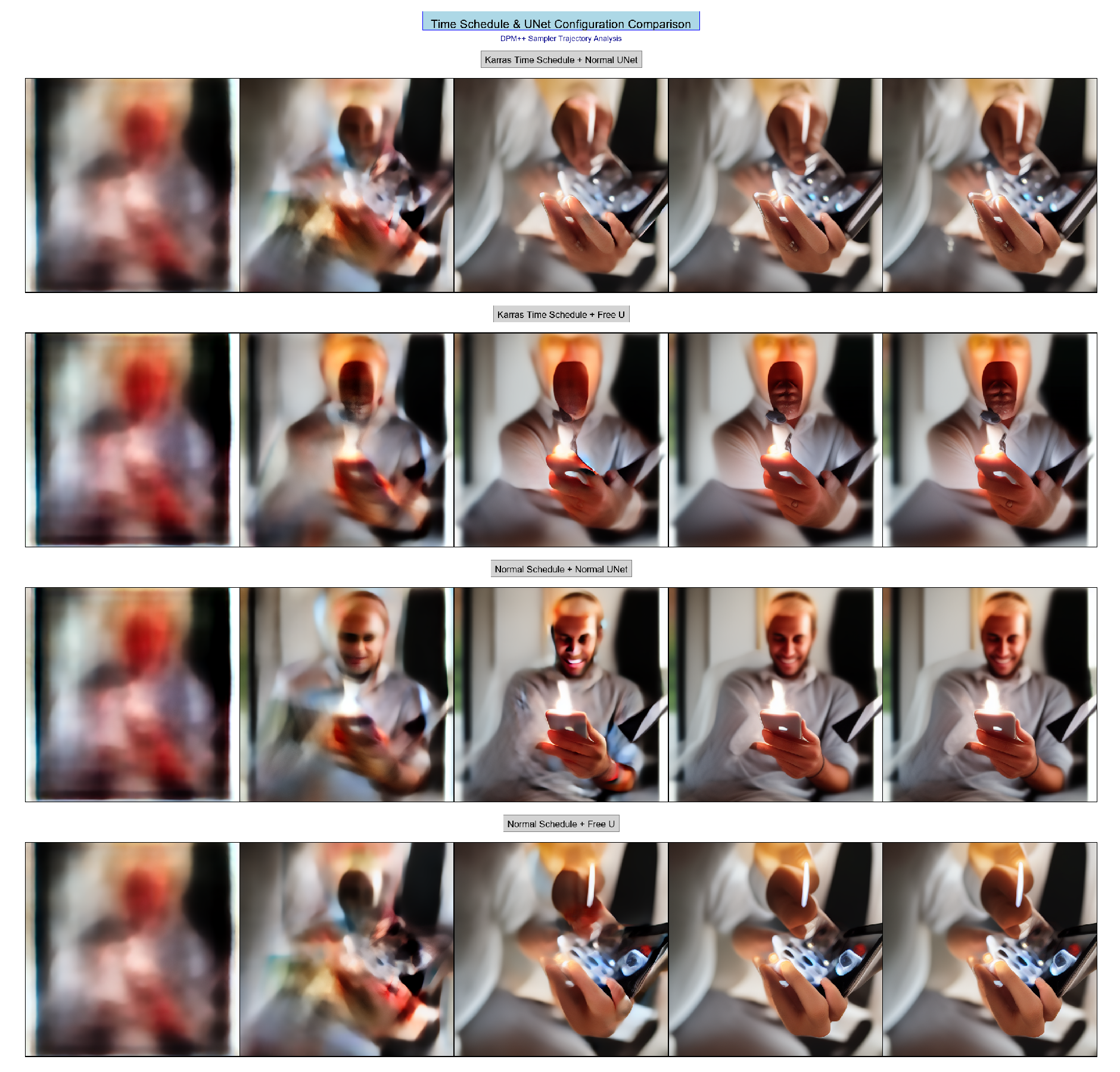
We then visualize the decode trajectory of using different discrete methods by applying the same sampler DPM++ 1s sampler in Figure 4. The normal time schedule using Free-U will generate a trajectory similar to the method using Karras’ time schedule without using Free-U, which exhibits the evidence of our previous claim.
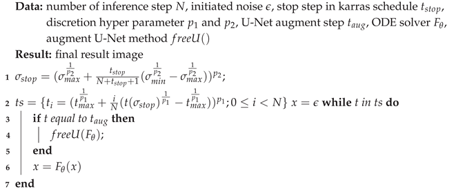
Our algorithm can be described by the tab:alorithm
| Algorithm 1: custom Karras scheduler in the common framework of Diffusion ODE solving |
 |
3.2. Information Theory Analysis of the Different Algorithms
A common point of confusion in deep learning at an early age is how neural networks with so many parameters still have generalization ability[35]. The normal statistical model uses an extremely limited number of parameters to ensure that it can concisely describe the phenomenon and capture the essence of the observed data. For this problem, the study theory[36] claims that limiting the number of functions that a model can express helps ensure that the model approaches the best functions it can have, and that it also bounds the distance between the final function a neural network study about and the average of functions. Generally, a possible function expressed by a model is a hypothesis , and if the number of input data points is N, the number of possible hypotheses is less than . According to the information theory, for a dataset with data D, the typical set that a model can gain access to is [37]. Considering the amount of data in the typical set, and the mutual information between the output and the middle feature of the neural network , we can further bound the models’ capacity for potential hypotheses.
Explicitly, we can consider the probability of middle feature z given output y, and the provides a match between y and z. The information bottleneck theory[38] shows that denotes the volume of Y project to the Z. Hence, further constraints the possible hypotheses. As the mutual information bounds the distance between the study hypothesis and the average hypothesis, generative adversarial networks (GANs) [39], which face mode collapse[40] that only generate a subset of the dataset, can benefit from it by adding a mutual information constraint [41]. One study[26] shows that this phenomenon also appears in the diffusion distillation, which consistently changes the score function and triggers an increase in mutual information. The basic idea of the proof in that study is related to -variation auto-encoder (-VAE)[30], in which, when -VAE decreases to let VAE generate high-quality images, the upper bounce of the mutual information constraint will be abated, and there will be an increase in the peak signal-to-noise ratio (PSNR) of the encoding feature Z. From this perspective, the diffusion model can be deemed as a hierarchy VAE[4], while progressive distillation[15] increases the mutual information by letting the model directly use to replace the original output . Where is a noisy feature output by solving ODE. Hence, the PSNR also increases. A recent example of diffusion distillation is SDXL-lightning[12], which adds GAN loss to the progressive distillation training, and its FID remains similar to normal progressive distillation.
However, it is intuitive that changing the direction of the score function to allow it to point to the final result, rather than the centroid of the possible image, will also affect the mutual information, even if the output does not have an increased PSNR. We provide further analysis regarding this.
The diffusion ODE can be regarded as a Markov process , in which follows the input of the diffusion model predicted by the U-Net, and we have the following Equation (23):
in which is the real sample from the dataset.
In -VAE, when given the random variable Z, the output Y is assumed to be sampled from a Gaussian distribution using Y as its mean, and abating the makes the middle feature Z more similar to Y while enhancing the log likelihood of the final synthesis. Moreover, Equation (23) shows that if we modify the to make it similar to the final output to enhance the log-likelihood by rectifying the trajectory, then the upper bound of the mutual information will also increase. Most distillation methods that do not increase the PSNR of the output will still face this problem. We evaluate the Precision and Recall of Distribution (PRD)[42] of flash diffusion and our sampler to further validate this claim.
4. Experiments
4.1. Performance
In this study, we employ , , , and as the hyperparameters of the discrete setting in the eight-step inference when generating 1024 x 1024 and 512 x 512 images. For the eight-step inference, as the precise discretization method, we can completely avoid using free-U, which can enhance the aesthetic of images while reducing its FID in the few-step inference. We report the results of the eight-step inference in the COCO 2014, COCO 2017, and LAION dataset in Table 1, Table 2, and Table 3. Moreover, we use , as the setting in the five- and six-step inference of generating 512 x 512 images and the six-step inference of generating 1024 x 1024 images. The result of the five- and six-step inference that synthesizes 512 x 512 images is also given in Table 1, Table 2, and Table 3. Moreover, the result of the 1024 x 1024 images is given in Table 4, Table 5, and Table 6. The free-U is used throughout the inference when we sample a 512 x 512 image, and it is used in the last three steps when we synthesize a 1024 x 1024 image. Moreover, the ODE solver, based on the analysis in Section 3, is DPM++2m for eight-step inference and DPM++1s for five-step inference. The inference model that uses our algorithm for synthesizing 512 x 512 images and 1024 x 1024 images is Stable Diffusion v1.5 and Dreamshaper XL, respectively. In the generation of 1024 x 1024 images in 6 steps, we use the SDE-Editing method mentioned in the paper[43]. Furthermore, all the synthesized images in Table 1 and Table 4 employs the random 10k COCO caption as a guidance prompt. In Table 2 and Table 5, for each image in the COCO 2017 dataset, we fetch one particular caption of it as guidance. Furthermore, we use 10k captions in LAION for Table 3 and Table 6. We also compare the FID performance and the clip score of AMED-Pulging solver, progressive distillation, SDXL turbo, SDXL-Lightning, Flash DiffusionXL, Flash Diffusion, and DMD2[12,14,16,44]. Our approach outperforms state-of-the-art models for most of the datasets. However, some of the models[14] are trained in LAION, which do not separate the validation and the training sets, and may affect the comparison. The w in the Table 1 and Table 4 is the guidance scale of inference, and the number in the parentheses is the total number of function evaluations (NFEs) of the model. The , , , and in the Free-U decorator is 1.1, 1.1, 0.9, 0.2.

Table 1.
Results of 512 x 512 image generation. COCO 2014
| Solver | FID | CLIP-Score |
|---|---|---|
| (Our) custom DPM++1s(5) | 19.18 | 30.92 |
| (Our) custom DPM++1s(6) | 18.54 | 31.16 |
| (Our) custom DPM++2m(8) | 15.92 | 31.32 |
| (Our) custom DPM++1s(5) | 17.54 | 31.0 |
| (Our) custom DPM++1s(6) | 17.04 | 31.16 |
| (Our) custom DPM++2m(8) | 15.7 | 31.07 |
| Original DPM++2m(20) | 17.3 | 30.97 |
| Original DPM++2m(20) | 18.68 | 30.97 |
| Flash Diffusion(5) | 17.34 | 30.45 |
| Flash Diffusion(6) | 17.94 | 30.59 |
| Flash Diffusion(8) | 19.03 | 30.37 |
| AMED Pulgin(8) | 19.07 | 31.15 |
| SDXL turbo(4) | 23.24 | 31.66 |
Table 2.
Results of 512 x 512 image generation. COCO 2017
| Solver | FID | CLIP-Score |
|---|---|---|
| (Our) custom DPM++1s(5) | 24.22 | 31.06 |
| (Our) custom DPM++1s(6) | 23.24 | 31.12 |
| (Our) custom DPM++2m(8) | 22.40 | 31.23 |
| (Our) custom DPM++1s(5) | 25.58 | 30.93 |
| (Our) custom DPM++1s(6) | 24.71 | 31.13 |
| (Our) custom DPM++2m(8) | 22.35 | 31.35 |
| Original DPM++2m(20) | 25.97 | 31.21 |
| Original DPM++2m(20) | 23.75 | 31.10 |
| Flash Diffusion(5) | 23.56 | 30.64 |
| Flash Diffusion(6) | 24.16 | 30.60 |
| Flash Diffusion(8) | 25.35 | 30.55 |
| AMED Pulgin(8) | 25.50 | 31.17 |
| SDXL turbo(4) | 30.92 | 31.66 |
Table 3.
Results of 512 x 512 image generation. Laion
| Solver | FID | CLIP Score |
|---|---|---|
| (Our) custom DPM++1s(5) | 19.61 | 31.81 |
| (Our) custom DPM++1s(6) | 18.45 | 32.10 |
| (Our) custom DPM++2m(8) | 17.74 | 32.42 |
| (Our) custom DPM++1s(5) | 19.88 | 31.45 |
| (Our) custom DPM++1s(6) | 18.60 | 31.97 |
| (Our) custom DPM++2m(8) | 17.52 | 32.41 |
| Original DPM++2m(20) | 18.30 | 32.67 |
| Original DPM++2m(20) | 17.33 | 32.47 |
| Flash Diffusion(5) | 15.40 | 31.60 |
| Flash Diffusion(6) | 15.80 | 31.63 |
| Flash Diffusion(8) | 16.87 | 31.57 |
| AMED Pulgin(8) | 18.06 | 32.44 |
| SDXL turbo(4) | 22.25 | 33.02 |
Table 4.
Results of 1024 x 1024 image generation. COCO 2014
| Solver | FID | CLIP Score |
|---|---|---|
| custom DPM++2m (8) | 17.84 | 31.62 |
| custom DPM++2m (8) | 19.62 | 31.58 |
| custom DPM++1s (6) | 23 | 31.23 |
| custom DPM++1s (6) | 24.25 | 31.49 |
| Flash DiffusionXL (6) | 22.23 | 31.00 |
| Flash DiffusionXL (8) | 23.25 | 30.89 |
| SDXL-Lightning (8) | 21.07 | 31.11 |
| DMD2 (4) | 19.64 | 31.64 |
Table 5.
Results of 1024 x 1024 image generation. COCO 2017
| Solver | FID | CLIP Score |
|---|---|---|
| custom DPM++2m (8) | 24.42 | 31.71 |
| custom DPM++2m (8) | 26.04 | 31.56 |
| custom DPM++1s (6) | 29.52 | 31.15 |
| custom DPM++1s (6) | 30.51 | 31.47 |
| Flash DiffusionXL (6) | 28.74 | 30.96 |
| Flash DiffusionXL (8) | 29.63 | 30.88 |
| SDXL-Lightning (8) | 27.89 | 31.08 |
| DMD2 (4) | 26.19 | 31.65 |
Table 6.
Results of 1024 x 1024 image generation.Laion
| Solver | FID | CLIP Score |
|---|---|---|
| custom DPM++2m (8) | 19.25 | 32.22 |
| custom DPM++2m (8) | 20.82 | 32.07 |
| custom DPM++1s (6) | 20.94 | 31.01 |
| custom DPM++1s (6) | 22.10 | 31.59 |
| Flash DiffusionXL (6) | 20.88 | 31.64 |
| Flash DiffusionXL (8) | 21.30 | 31.61 |
| SDXL-Lightning (8) | 20.45 | 32.50 |
| DMD2 (4) | 16.51 | 33.28 |
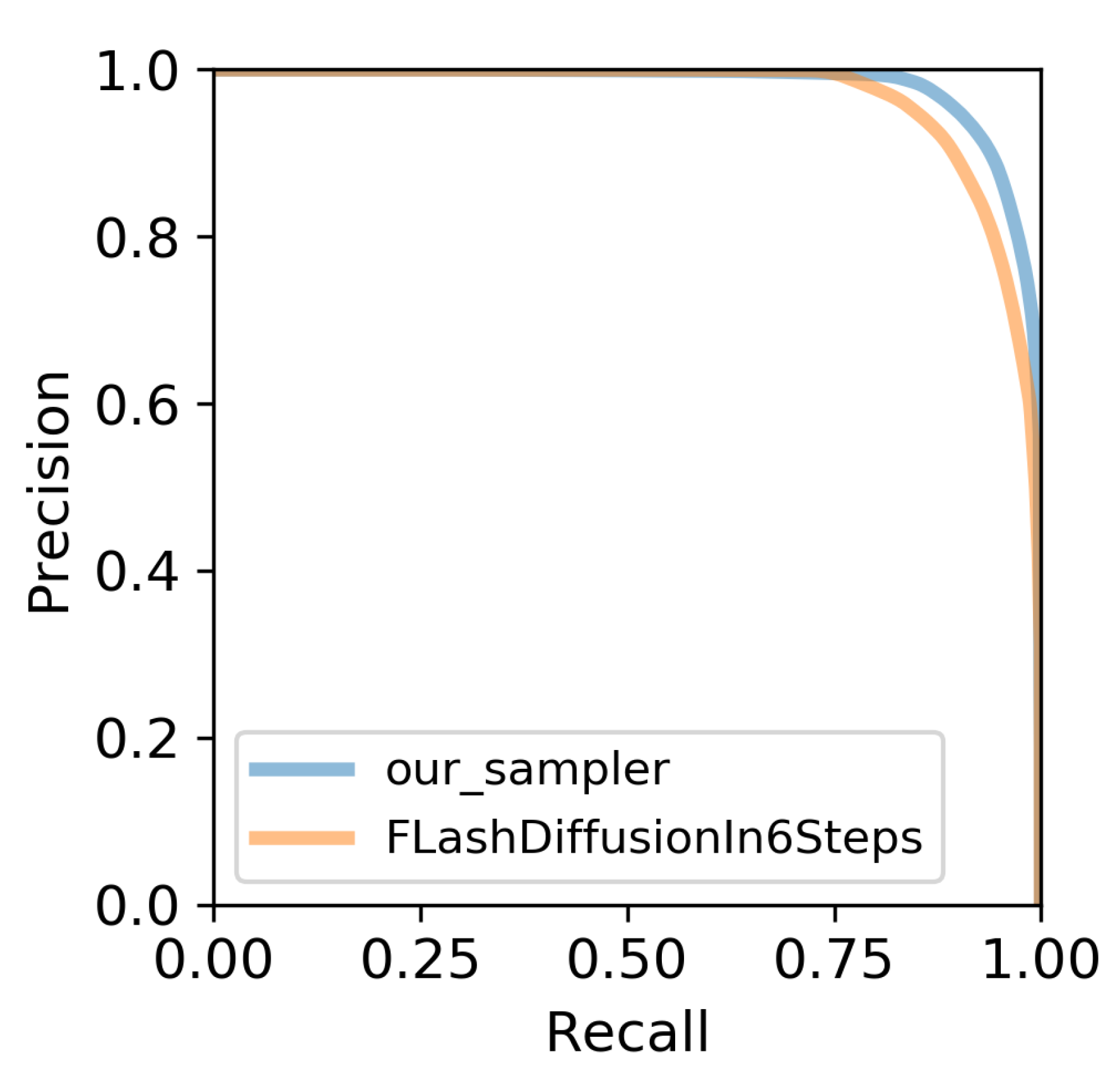
We also calculate the PRD in a 6-step inference by sampling 10k captions from COCO 2014 and getting the corresponding image in the COCO dataset as a reference. PRD was first used to evaluate GAN. Considering two distributions Q and P, the first one is the distribution of the generative images, and the second one is the distribution of the original images, the precision shows how much of Q can be generated by P, and the recall exhibits how much P can be generated by Q. For example, if P is a subset of MNIST that only contains numbers ranging from 1 to 4, adding 5 and 6 to the generative distribution reduces the precision, while lacking modes like 3 and 4 will reduce the recall rate. Our experiment shows that the recall rate of the flash diffusion in the 6-step is less than that of us. The guidance scale of our sampler is 5.
Figure 5.
The comparison of PRD between our 6-step inference sampler and the FLash diffusion.
5. Conclusion
In this study, we propose a plug-in method to enhance the sampling algorithm. By fully harnessing the potential capacity of the latent diffusion model—such as modifying the skip-connection at the right time, using the property of the decoder, which is a -VAE trained with small KL-constraints, ignoring a small amount of noise in the final feature to reschedule the discretizing method, and choosing the proper ODE solver via truncation error analysis—we can sample a high-quality image with limited inference budget and avoid the need for additional training.
5.1. Limitation and the Future Work
A diffusion model is a robust generative model[45] that can prevent adversarial attacks. Most attacks that hack the latent diffusion model attack its VAE decoder. Thus, it remains unclear whether the robustness of the diffusion model will be affected when using our algorithm in a scenario that mainly depends on the property of the VAE. Moreover, in future research, we explore whether it is possible to find a better scheduler in a low-step inference process via an automated algorithm, and whether this new time scheduler is available to different latent diffusion models.
Acknowledgments
We thank LetPub (www.letpub.com.cn) for its linguistic assistance during the preparation of this manuscript.
References
- Ho, J.; Jain, A.; Abbeel, P. Denoising diffusion probabilistic models. Advances in neural information processing systems 2020, 33, 6840–6851.
- Rombach, R.; Blattmann, A.; Lorenz, D.; Esser, P.; Ommer, B. High-resolution image synthesis with latent diffusion models. In Proceedings of the Proceedings of the IEEE/CVF conference on computer vision and pattern recognition, 2022, pp. 10684–10695.
- Song, Y.; Sohl-Dickstein, J.; Kingma, D.P.; Kumar, A.; Ermon, S.; Poole, B. Score-based generative modeling through stochastic differential equations. arXiv preprint arXiv:2011.13456 2020.
- Luo, C. Understanding diffusion models: A unified perspective. arXiv preprint arXiv:2208.11970 2022.
- Lu, C.; Zhou, Y.; Bao, F.; Chen, J.; Li, C.; Zhu, J. Dpm-solver++: Fast solver for guided sampling of diffusion probabilistic models. Machine Intelligence Research 2025, pp. 1–22.
- Song, J.; Meng, C.; Ermon, S. Denoising diffusion implicit models. arXiv preprint arXiv:2010.02502 2020.
- Zhao, W.; Bai, L.; Rao, Y.; Zhou, J.; Lu, J. Unipc: A unified predictor-corrector framework for fast sampling of diffusion models. Advances in Neural Information Processing Systems 2023, 36, 49842–49869.
- Karras, T.; Aittala, M.; Aila, T.; Laine, S. Elucidating the design space of diffusion-based generative models. Advances in neural information processing systems 2022, 35, 26565–26577.
- Liu, L.; Ren, Y.; Lin, Z.; Zhao, Z. Pseudo numerical methods for diffusion models on manifolds. arXiv preprint arXiv:2202.09778 2022.
- Luo, S.; Tan, Y.; Patil, S.; Gu, D.; Von Platen, P.; Passos, A.; Huang, L.; Li, J.; Zhao, H. Lcm-lora: A universal stable-diffusion acceleration module. arXiv 2023. arXiv preprint arXiv:2311.05556.
- Song, Y.; Dhariwal, P. Improved techniques for training consistency models. arXiv preprint arXiv:2310.14189 2023.
- Lin, S.; Wang, A.; Yang, X. Sdxl-lightning: Progressive adversarial diffusion distillation. arXiv preprint arXiv:2402.13929 2024.
- Yin, T.; Gharbi, M.; Zhang, R.; Shechtman, E.; Durand, F.; Freeman, W.T.; Park, T. One-step diffusion with distribution matching distillation. In Proceedings of the Proceedings of the IEEE/CVF conference on computer vision and pattern recognition, 2024, pp. 6613–6623.
- Yin, T.; Gharbi, M.; Park, T.; Zhang, R.; Shechtman, E.; Durand, F.; Freeman, B. Improved distribution matching distillation for fast image synthesis. Advances in neural information processing systems 2024, 37, 47455–47487.
- Salimans, T.; Ho, J. Progressive distillation for fast sampling of diffusion models. arXiv preprint arXiv:2202.00512 2022.
- Sauer, A.; Lorenz, D.; Blattmann, A.; Rombach, R. Adversarial diffusion distillation. In Proceedings of the European Conference on Computer Vision. Springer, 2024, pp. 87–103.
- Kim, D.; Lai, C.H.; Liao, W.H.; Murata, N.; Takida, Y.; Uesaka, T.; He, Y.; Mitsufuji, Y.; Ermon, S. Consistency trajectory models: Learning probability flow ode trajectory of diffusion. arXiv preprint arXiv:2310.02279 2023.
- Song, Y.; Dhariwal, P.; Chen, M.; Sutskever, I. Consistency models 2023.
- Liu, X.; Zhang, X.; Ma, J.; Peng, J.; et al. Instaflow: One step is enough for high-quality diffusion-based text-to-image generation. In Proceedings of the The Twelfth International Conference on Learning Representations, 2023.
- Heusel, M.; Ramsauer, H.; Unterthiner, T.; Nessler, B.; Hochreiter, S. Gans trained by a two time-scale update rule converge to a local nash equilibrium. Advances in neural information processing systems 2017, 30.
- Lin, T.Y.; Maire, M.; Belongie, S.; Hays, J.; Perona, P.; Ramanan, D.; Dollár, P.; Zitnick, C.L. Microsoft coco: Common objects in context. In Proceedings of the European conference on computer vision. Springer, 2014, pp. 740–755.
- Schuhmann, C.; Beaumont, R.; Vencu, R.; Gordon, C.; Wightman, R.; Cherti, M.; Coombes, T.; Katta, A.; Mullis, C.; Wortsman, M.; et al. Laion-5b: An open large-scale dataset for training next generation image-text models. Advances in neural information processing systems 2022, 35, 25278–25294.
- Ho, J.; Jain, A.; Abbeel, P. Denoising diffusion probabilistic models. Advances in neural information processing systems 2020, 33, 6840–6851.
- Lu, C.; Zhou, Y.; Bao, F.; Chen, J.; Li, C.; Zhu, J. Dpm-solver: A fast ode solver for diffusion probabilistic model sampling in around 10 steps. Advances in neural information processing systems 2022, 35, 5775–5787.
- Ho, J.; Salimans, T. Classifier-free diffusion guidance. arXiv preprint arXiv:2207.12598 2022.
- Li, Z.; Zhang, R. Direct Distillation: A Novel Approach for Efficient Diffusion Model Inference. Journal of Imaging 2025, 11, 66.
- Ronneberger, O.; Fischer, P.; Brox, T. U-net: Convolutional networks for biomedical image segmentation. In Proceedings of the International Conference on Medical image computing and computer-assisted intervention. Springer, 2015, pp. 234–241.
- Vaswani, A.; Shazeer, N.; Parmar, N.; Uszkoreit, J.; Jones, L.; Gomez, A.N.; Kaiser, Ł.; Polosukhin, I. Attention is all you need. Advances in neural information processing systems 2017, 30.
- Li, Z.; Liu, F.; Yang, W.; Peng, S.; Zhou, J. A survey of convolutional neural networks: analysis, applications, and prospects. IEEE transactions on neural networks and learning systems 2021, 33, 6999–7019.
- Burgess, C.P.; Higgins, I.; Pal, A.; Matthey, L.; Watters, N.; Desjardins, G.; Lerchner, A. Understanding disentangling in backslash beta-vae. arXiv preprint arXiv:1804.03599 2018, 2.
- Wu, H.; Flierl, M. Vector quantization-based regularization for autoencoders. In Proceedings of the Proceedings of the AAAI Conference on Artificial Intelligence, 2020, Vol. 34, pp. 6380–6387.
- Si, C.; Huang, Z.; Jiang, Y.; Liu, Z. Freeu: Free lunch in diffusion u-net. In Proceedings of the Proceedings of the IEEE/CVF Conference on Computer Vision and Pattern Recognition, 2024, pp. 4733–4743.
- He, K.; Zhang, X.; Ren, S.; Sun, J. Deep residual learning for image recognition. In Proceedings of the Proceedings of the IEEE conference on computer vision and pattern recognition, 2016, pp. 770–778.
- Chen, R.T.; Rubanova, Y.; Bettencourt, J.; Duvenaud, D.K. Neural ordinary differential equations. Advances in neural information processing systems 2018, 31.
- Breiman, L. Reflections after refereeing papers for nips. In The Mathematics of Generalization; CRC Press, 2018; pp. 11–15.
- Harman, G.; Kulkarni, S. Reliable reasoning: Induction and statistical learning theory; MIT press, 2012.
- Yeung, R.W. A first course in information theory; Springer Science & Business Media, 2012.
- Tishby, N.; Pereira, F.C.; Bialek, W. The information bottleneck method. arXiv preprint physics/0004057 2000.
- Goodfellow, I.; Pouget-Abadie, J.; Mirza, M.; Xu, B.; Warde-Farley, D.; Ozair, S.; Courville, A.; Bengio, Y. Generative adversarial networks. Communications of the ACM 2020, 63, 139–144.
- Creswell, A.; White, T.; Dumoulin, V.; Arulkumaran, K.; Sengupta, B.; Bharath, A.A. Generative adversarial networks: An overview. IEEE signal processing magazine 2018, 35, 53–65.
- Jeon, I.; Lee, W.; Pyeon, M.; Kim, G. Ib-gan: Disentangled representation learning with information bottleneck generative adversarial networks. In Proceedings of the Proceedings of the AAAI conference on artificial intelligence, 2021, Vol. 35, pp. 7926–7934.
- Sajjadi, M.S.; Bachem, O.; Lucic, M.; Bousquet, O.; Gelly, S. Assessing generative models via precision and recall. Advances in neural information processing systems 2018, 31.
- Podell, D.; English, Z.; Lacey, K.; Blattmann, A.; Dockhorn, T.; Müller, J.; Penna, J.; Rombach, R. Sdxl: Improving latent diffusion models for high-resolution image synthesis. arXiv preprint arXiv:2307.01952 2023.
- Chadebec, C.; Tasar, O.; Benaroche, E.; Aubin, B. Flash diffusion: Accelerating any conditional diffusion model for few steps image generation. In Proceedings of the Proceedings of the AAAI Conference on Artificial Intelligence, 2025, Vol. 39, pp. 15686–15695.
- Chen, H.; Dong, Y.; Shao, S.; Hao, Z.; Yang, X.; Su, H.; Zhu, J. Your diffusion model is secretly a certifiably robust classifier. arXiv preprint arXiv:2402.02316 2024.
Figure 1.
The comparison between our algorithm and dpm++ solver in few step inference
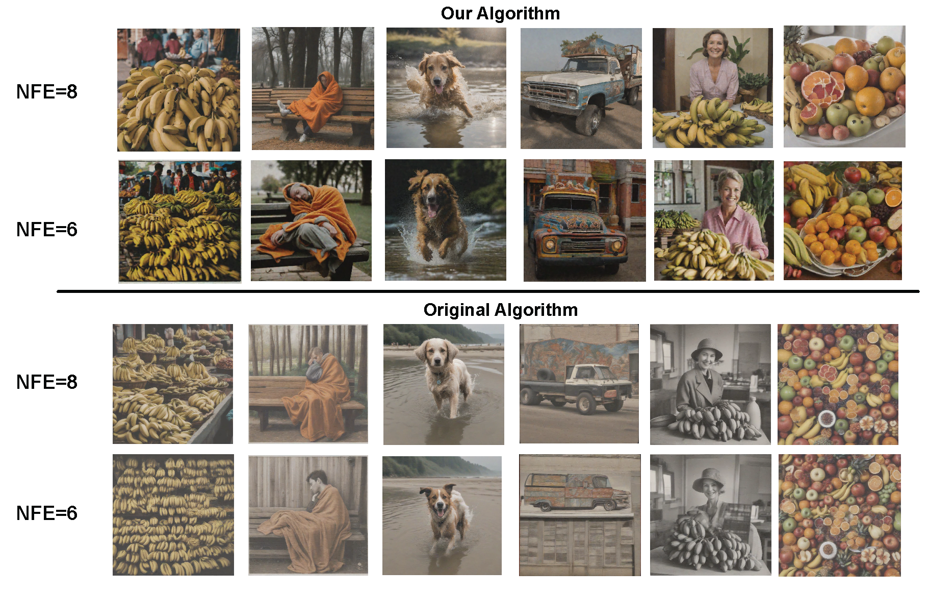
Figure 2.
The comparison between our time schedule and the time schedule proposed by Karras
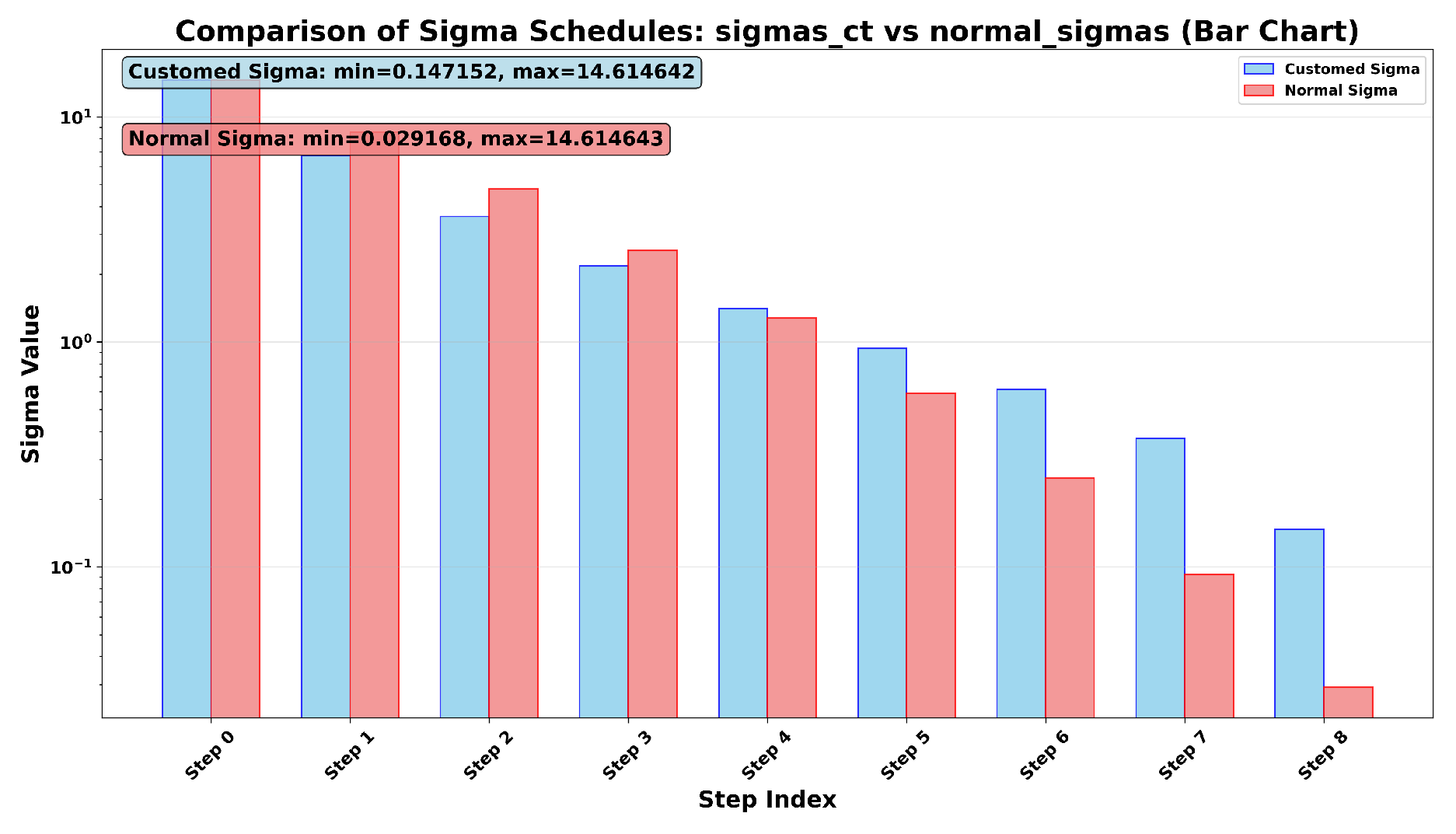
Figure 3.
The comparison between our sampler and the original DPM++1s sampler. The first line is the result trajectory of the original DPM++1s sampler with Karras’ schedule, the second one is Karras’ schedule + Free-U, and the last one is our sampler. The results show that if we apply Free-U in a few-step sampling without involving additional tricks, the generation result will be degraded.
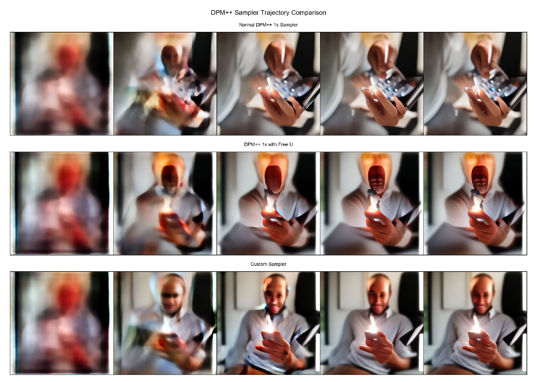
Figure 4.
The comparison between different discrete method when using the same DPM++ 1s Sampler in a few-step inference. The first line exhibit the trajectory of the normal Karras discrete method. The second one exhibit the trajectory of the Karras discrete method + Free-U. The third exhibite the normal discrete method with normal U-Net, and the final one exhibit the normal discrete method with Free-U. And the final line is similiar to the first line.
Disclaimer/Publisher’s Note: The statements, opinions and data contained in all publications are solely those of the individual author(s) and contributor(s) and not of MDPI and/or the editor(s). MDPI and/or the editor(s) disclaim responsibility for any injury to people or property resulting from any ideas, methods, instructions or products referred to in the content. |
© 2025 by the authors. Licensee MDPI, Basel, Switzerland. This article is an open access article distributed under the terms and conditions of the Creative Commons Attribution (CC BY) license (http://creativecommons.org/licenses/by/4.0/).
Copyright: This open access article is published under a Creative Commons CC BY 4.0 license, which permit the free download, distribution, and reuse, provided that the author and preprint are cited in any reuse.


