
Submitted:
22 September 2025
Posted:
24 September 2025
You are already at the latest version
Abstract
The urban heat island (UHI) has been a critical social problem as urbanization intensifies worldwide, significantly impacting human life by exacerbating heat-related health issues, increasing energy demand for cooling and the associated environmental problems. To accurately assess the risk of heat intensification for human health and ecosystem, it is important to quantify the significance at specific times and locations. However, there have been little analyses that capture both the diurnal and spatial variations due to the limitations of traditional satellite datasets. This study investigates the fine-scale spatio-temporal behaviors of the heat island effect in Korea's most heat-impacted metropolitan cities, by utilizing relatively new land surface temperature (LST) data: ECOsystem Spaceborne Thermal Radiometer Experiment on Space Station (ECOSTRESS). The analysis demonstrated that our high-resolution assessment revealed surface urban heat island (SUHI) intensities during summer to be 5–8 ℃ higher compared to those derived from coarse-resolution data. The intensification rates by land uses were also quantified with greater accuracy, showing that industrial areas experienced changes of up to roughly 2 ℃/hour during the early morning in summer. The spatial characteristics of heat intensification were examined across various land use types, revealing that densely clustered urban land uses can amplify heat intensification, with industrial areas experiencing a doubling effect.
Keywords:
surface urban heat island
; sub-district level
; diurnal variation
; Busan
; Daegu
1. Introduction
As urban areas have gradually expanded since the early phase of industrialization in the 19th century, impervious surfaces dramatically increased and led to significant modifications in the thermodynamics of urban environments [1,2]. Combined with extreme heatwaves that have recently become more frequent and intense as a part of global climate change, the urban heat island (UHI) effect now threatens human lives by increasing demands for water and energy, escalating heat-related mortality, and even altering regional climates [3,4,5]. The adverse effects are expected to worsen under current warming trends if no proper urban adaptation strategies are implemented [6,7].
UHI can be classified into two main types based on the location of heat intensification: atmospheric UHI (AUHI) and surface UHI (SUHI) [8,9,10]. AUHI, quantified using air temperature measurements from meteorological stations and radiosondes, has significant implications for human health and air pollution, typically affecting larger areas and being most pronounced during nighttime [11,12]. In contrast, SUHI, derived from surface temperature measurements, exhibits higher spatial variability and temperature ranges compared to AUHI, as it strongly depends on surface materials and land uses [13,14,15]. SUHI has a closer connection to human perception of heat intensification, influencing heat-related illnesses, energy consumption for cooling, and surface thermodynamic processes such as evapotranspiration [3,5,11,16,17]. An advantage of studying SUHI is the feasibility of spatial analysis, as land surface temperature (LST) data are readily available in image format from satellite observations [18,19].
While SUHI primarily involves urban-scale assessments of surface temperature relative to adjacent rural areas, understanding fine-scale spatial and temporal variations within urban areas is essential for evaluating their effects on humans and ecosystem [20,21]. We refer to such fine-scale SUHI behavior at the sub-district level as locational heat intensification (LHI), to differentiate from SUHI which is typically evaluated over the entire urban area. Studies have shown that urban heat intensity varies significantly within cities, driven by factors such as land use, vegetation cover, topography, and building materials, creating temperature differences of up to several degrees between neighbourhoods [22,23]. Additionally, spatiotemporal analyses have demonstrated that areas with higher LHI often overlap with regions experiencing elevated air pollution levels, which correlate strongly with increased incidences of respiratory and cardiovascular diseases in affected populations [11]. However, analysis on LHI remain challenging in most urban areas due to limitations in observational data that offer both continuity and high spatial resolution.
The lack of fine-scale analysis is also evident in Busan and Daegu, two metropolitan cities in Korea that are highly vulnerable to heatwaves and the tropical night phenomenon [24,25]. Busan and Daegu report respectively the highest incidence of heat-related illnesses per capita [26], and the most frequent heatwave events in Korea [27]. Despite previous efforts to characterize SUHI patterns in Busan and Daegu, a significant research gap persists in understanding the diurnal variation of temperature influenced by land use. Coarse-scale SUHI characteristics have been identified for these cities using Landsat-8 LST data [28], but the analysis is restricted to a fixed time in the morning (~11:00), leaving the thermal behavior during peak afternoon hours unexplored. While Moderate Resolution Imaging Spectroradiometer (MODIS) day/night LST data [29,30] and LST data from geostationary satellites such as Communication, Oceanography and Meteorology Satellite (COMS) have been employed to observe hourly LST variations, their coarse spatial resolution limits the ability to conduct sub-district-level analyses that account for the highly variable nature of urban land uses [31,32,33]. Multiple attempts have been made to upsample the LST data by using techniques such as super resolution, spatial downscaling, or temporal interpolation [32,34,35,36,37,38,39,40], but each of these techniques tends to introduce high uncertainty that can lead to misleading results in UHI interpretation [41].
This study presents the first-ever analysis of the spatio-temporal breakdown of SUHI, for Busan and Daegu, revealing the diurnal effect at the sub-district level. High-resolution ECOsystem Spaceborne Thermal Radiometer Experiment on Space Station (ECOSTRESS) LST data (70 meters) were utilized to capture diurnal LST timestamps across various dates, which were composited to represent the season-specific diurnal patterns. Since the season-representative diurnal temperature pattern can be derived from ECOSTRESS data from multiple dates, we employed a compensation scheme that utilizes LST data from geostationary satellite to remove the daily variation in the multi-day ECOSTRESS data. For geostationary data, this study used Geostationary Korea Multi-Purpose Satellite-2A (GK-2A) which produces LST data over the Korean peninsula every 30 minutes.
This study had three primary objectives. First, the diurnal variations of SUHI and LST in the two cities were examined across all four seasons. Urban-scale diurnal SUHI patterns were derived from ECOSTRESS data and compared with SUHI estimates from GK-2A LST data, which are known to underestimate SUHI due to spatial averaging effects [20,33]. Additionally, the diurnal variation of LST was analyzed for individual land use types to highlight differences in heating and cooling rates, timing, and magnitude across these land uses, which are caused by spatial resolution. Second, spatial analysis was conducted using LHI maps generated at different hours during summer for the two cities. The spatial distribution of hot spots was analyzed to demonstrate the contributions of specific land uses and locations to SUHI. Additionally, the effect of land-use agglomeration was assessed to determine how spatial density influences LHI at the sub-district level. Finally, the results were compared between the two cities to identify differences in the temporal and spatial patterns of SUHI and LHI.
The manuscript is structured as follows. The Data section introduces the datasets, including both satellite and field measurements. The Method section outlines the process for combining ECOSTRESS and GK-2A data for the calculation of season-representative SUHI and LHI. In the Results section, the analysis on SUHI variation for the two cities is presented. The Discussion section addresses the potential causes and implications of the findings. Finally, the Conclusion provides an overall summary of the study and discusses directions for future research.
2. Materials
2.1. Study Area
Busan, located at 35° 10′ 46″ N and 129° 4′ 32″ E, is the second-largest metropolitan city in South Korea and the country’s premier maritime hub, with a population of approximately 3.4 million and the gross regional domestic product per capita of roughly 24,000 USD as of 2022 (Figure 1) [42]. For the past 5 years (2018–2022), the highest monthly mean air temperature was 26.9 ℃ in August, followed by 25.1 ℃ in July. The annual precipitation was 1,696 mm, and the precipitation in July and August 4 amounted to 641 mm, accounting for 37.8% of the total annual amount of precipitation [43]. Unlike Daegu, which is located in a basin, Busan includes mountains and hills within the city, restricting the built-up areas to narrow low-level flat areas surrounded by the ridges. As of 2023, the population ratio of people over age 65 is 22.2%, which is the highest in Korea [44]. Furthermore, between 2013 and 2022, Busan recorded an average of 21.8 heat-related illness cases per million people, marking the highest incidence among the seven metropolitan cities [26].
Daegu is located at 35° 52′ 20″ N, 128° 36′ 9″ E, and has a population of approximately 2.4 million and a gross regional domestic product per capita of roughly 20,000 USD as of 2022 (Figure 1) [45]. The monthly mean air temperature record for the past 5 years (2018–2022) shows that the lowest temperature was 1.2 ℃ in January, and the highest was 27.3 ℃ in August, with a maximum temperature of 39.2 ℃ during that period. The yearly mean number of heatwave days (defined as days when the maximum temperature exceeds 33 ℃) for the period was 33.6 days with the longest lasting 26 days in 2018. Annual precipitation was approximately 1005 mm for the 5 years, and precipitation for the two hottest months, July and August, was 397 mm, accounting for 43.8% of the total precipitation [43]. Daegu is located in a basin formed by Palgong Mountain (1,193 m) in the north and Biseul Mountain (1,084 m) in the south. A northwesterly wind is dominant in summer.
Both cities fall into the temperate climate zone, experiencing four distinct seasons. Although Busan is further south than Daegu, Busan’s summer is cooler than Daegu mainly due to its proximity to the ocean. Like other cities in Korea, the temperature record of the two cities clearly exhibits a warming trend, with the annual average temperature increasing at the rate of 0.18 ℃ per ten years for the period of 1912–2017 [46]. The aging index, defined as the ratio of the number of people greater than 65 years of age to the total population, was highest in Busan (22.2%) and the second highest in Daegu (19%) as of 2023 among the seven metropolitan cities in Korea including Seoul [44], indicating the susceptibility of the two cities to heat-related diseases.
2.2. Satellite Data
2.2.1. ECOSTRESS
ECOSTRESS is a space-borne thermal sensor with 6 spectral bands: 5 in the 8–12.56 µm range for temperature retrieval, and an extra band at 1.6 µm for geolocation and cloud detection. Because it is installed on the International Space Station, it revisits the same location in 1–5 days and provides LST data at a spatial resolution of 70 meters. LST data from ECOSTRESS were validated against field measurements at 14 global sites, revealing a root-mean-square error (RMSE) of 1.07 K and a mean average error of 0.40 K, with a cold bias of approximately 0.75 K for temperatures below 295 K [47]. For this study, we collected all available ECOSTRESS LST data for the southeastern region of Korea, covering the period from 2020 to 2022, while excluding images with more than 70% cloud cover. The data were sourced from NASA Earthdata (https://www.earthdata.nasa.gov/), with a total of 61 data points used across all seasons in this study. Detailed acquisition times are listed in the Appendix A.
2.2.2. GK-2A
The GK-2A satellite, launched in December 2018, is in a geostationary orbit at 128.2° E longitude. It captures images at 10-minute intervals across 16 spectral bands, ranging from the visible to the infrared. The LST products for Korea are available at a 2-km resolution with cloud pixels removed. These products have been cross-validated with synchronous MODIS LST data, revealing a bias of 1.227 K and an RMSE of 2.281 K. Further validation conducted using field data from the Tateno site in Japan, part of the baseline surface radiation network, showed that GK-2A LST has a bias of 0.523 K and an RMSE of 2.021 K [48]. In our study, GK-2A LST data for the period from 2020 to 2022 were collected at 30-minute intervals, specifically at the top of the hour and the half-hour, from the National Meteorological Satellite Center (https://nmsc.kma.go.kr/).
Before combining the two LST data sets, data from ECOSTRESS and GK-2A were compared for consistency. GK-2A LST data were resampled to the ECOSTRESS grid, which has a resolution of 70 meters. Figure 2 depicts the overall differences between the two LST data sets for the southeastern portion of Korea that includes Busan and Daegu. The pair of images in the upper row are for approximately 10:30 Korean Standard Time (KST) zone in the morning, and those in the bottom row are for the peak temperature at approximately 14:30 KST. Spatial variation in LST was much more evident in ECOSTRESS data than in GK-2A data for both pairs, and the pixels near the ocean and clouds were better preserved in ECOSTRESS. Figure 3 depicts scatter plots of LSTs derived from the two sensors for the urban core, suburban, and rural areas, respectively. The figure shows that the two LST data sets have a high correlation of greater than 0.98 for all area categories in a temperature range of 0–45 ℃. There is a positive bias in ECOSTRESS LST in high temperature range (> 35 ℃), which can be attributed to the difference in spatial resolution. The locations of the high temperature in ECOSTRESS LST data tend to be averaged out in the corresponding location in GK-2A, resulting in lower LST estimates.
2.3. Ancillary Data
2.3.1. Land Use Data
We used medium-level land use data provided by the Department of Environment of Korea to assess the SUHI effect by land use type. The data set, last updated in 2022, consists of 7 high-level types and 22 middle-level types with a spatial resolution of 5 meters. This data was produced with a classification accuracy standard of 95%, in accordance with the land use mapping guidelines issued by the Department of Environment of Korea. For analysis of heat islands, we recategorized the types into six effective types based on sufficiency in area and divergence in thermal behavior. Since the satellite LST products are not calibrated for water bodies, the Water Body class was excluded from the analysis [47]. Additionally, because the types with a few of pixels in the LST data may not be statistically significant, those with less than 3% coverage of the study area within both cities (e.g., Wet Land and Barren) were also excluded from the analysis. As a result, four high-level types: Built Area, Agricultural Land, Forest, and Grass were left for analysis. To investigate the differences within urban areas in more detail, we further divided the Built Area class into three medium-level types that are known to exhibit clearly different heat emission characteristics (e.g., Residential, Industrial, and Commercial) [49,50]. The six final land use classes used in this study are presented in Table 1. Land use maps of the two cities are displayed in Figure 4. In these maps, the Water Body class was displayed for illustrative purposes and was not considered for SUHI analysis. Pixels that do not fall into the six defined land use categories were aggregated into two additional classes based on their permeability (e.g., Pervious Mixed-Use, Impervious Mixed-Use) just for demonstration purposes. In this article, terms used as proper nouns, such as "Industrial Area," refer to specific areas of particular land uses defined on the map for calculating land-use-representative mean values, whereas terms used as common nouns, such as "industrial area(s)," refer to general areas serving such functions in urban settings.
2.3.2. Digital Elevation Model Data
Digital elevation model (DEM) data were obtained from the National Geographic Information Institute of Korea. DEM data, originally at a spatial resolution of 5 meters for all urban areas, were resampled to a 70-meter grid to match ECOSTRESS LST data. Based on the DEM, high-altitude mountainous areas (> 200 m) were screened from the evaluation of the SUHI effect to exclude the influences of elevation on city temperatures.
3. Method
3.1. Quantification of Urban-Scale SUHI Intensity
Urban-scale SUHI intensity (SUHII) was defined as the difference in LST between urban and rural areas, where the urban area was further divided into “urban core” and “suburban” based on the fraction of Built Area pixels. Specifically, the SUHII for the urban core () and suburban area () were calculated using Equations 1 and 2:
and represent the SUHII of the urban core and suburban areas, respectively, and , , indicate the LST of urban core, suburban, and rural areas. In this study, we defined urban and rural areas based on the criteria established by Schneider et al. [51,52,53] and classified regions by applying the methodology from Chang et al. [54] after adjusting the threshold values to fit the characteristics of our study area. Any location with more than 60% of Built Area pixels within a 1.5-km radius was classified as an urban core pixel, and areas with 20–60% built area pixels were classified as suburban. The rural area was defined as a 10-km buffer surrounding the urban areas. Areas with an elevation above 200 meters and water bodies such as rivers and oceans were excluded from the defined urban and rural areas for the reasons explained in the data section.
3.2. Derivation of Diurnal SUHI Variation
To derive mean LST time series representative for a season, daily adjustments were applied to every ECOSTRESS LST data, as implemented in Chang et al. [55]. Firstly, the daily deviation in LST at time on the day (i.e., ) is defined as the difference of LST at the particular timing from the seasonal mean LST (Equation 3):
where is the LST of time on day and is the seasonal mean LST which was calculated from all available data at of the season. Then, the adjusted daily LST at in (i.e., ) can be obtained by subtracting the daily deviation from the original LST measurements of the day, , as shown in Equation 4:
where we applied the adjustment to ECOSTRESS LST data of a particular timing. This adjustment assumes that the land uses are constant throughout the study period. Figure 5 depicts the effect of the daily adjustment by showing the histograms of day-to-day LST differences. LST scenes acquired on Oct. 12 and Oct. 30 in 2022 were selected for demonstration. It showed that bias of LST, which was -0.85 before the adjustment, became -0.20 after the adjustment, suggesting the effectiveness of the daily adjustment scheme.
3.3. Evaluation of LHI
The relative intensification of LST in a specific land use, compared to that of a rural area at the same time, is referred to as LHI, and is defined as in Equation 5:
where and are SUHI and LST specific to a land use, , respectively. Technically, the SUHI effect can be viewed as the spatial aggregation of LHI across the entire urban area. To derive at a specific time and location, an ECOSTRESS LST scene of the time was first processed for daily adjustment with respect to the GK-2A LST data of closest timing. To avoid a mixture of land use types in the evaluation, only the ECOSTRESS pixels (70-meter resolution) with more than 80% of a specific land use (5-meter resolution) were extracted and averaged for the calculation of at the scene. was calculated in the same manner as in the urban-scale SUHII evaluation to maintain consistency between the urban-scale and the sub-district-level LHI analysis. To calculate scene-representative diurnal LST, scenes that have valid pixels for fewer than 80% of the entire urban area were removed from the analysis.
3.4. Evaluation of the Land Use Density on the LHI
The density of a specific land use at a certain location, , was determined as the ratio of the number of pixels of the specific land use to that of others in an area within 300 meters of a specific area. The LHI of a specific land use for a certain density, , was calculated by subtracting the of the scene from the average LST for the specific land use at the specific land use density, , as shown in Equations 6, 7 and 8:
where only the pixels within the urban area are used for the averaging.
4. Results
4.1. Temporal Analysis of Urban Thermal Environment by Seasons
4.1.1. Diurnal Variation in SUHII at the Urban-Scale
A comparison of diurnal variation in the urban-scale SUHI effect is presented for each season of both cities in Figure 6. In all seasons, the variation captured by ECOSTRESS data was greater than that captured by GK-2A for both urban core and suburban areas. For example, in summer the peak SUHII of Daegu at around 14:00 was 10 ℃ with ECOSTRESS, which is 8 ℃ higher than that of GK-2A (2 ℃). This difference between ECOSTRESS and GK-2A can be observed in other seasons too, except for winter, which has too few data points due to frequent cloud cover. This implies that spatial resolution is a critical factor when assessing SUHII, even at the urban-scale. The differences by spatial resolution will be further investigated in the following LST analysis conducted for individual land uses.
The figure also indicates that the urban core SUHII captured by ECOSTRESS was not significantly different between spring and summer, particularly in Busan, despite higher overall LST levels in summer. The maximum urban core SUHII for Busan in both spring and summer was approximately 7 ℃, and Daegu's SUHII also reached 7 ℃ in summer. The peak timing of SUHI identified from the GK-2A time series was around 13:00 in both spring and summer, though it was less distinct in winter.
4.1.2. Land-Use-Specific LST Analysis at Sub-District-Level
Table 2 compares LST data from ECOSTRESS and GK-2, specifically for different land uses during summer. The LST estimates from the low-resolution satellite data (i.e. GK-2A) are smaller than that of high-resolution data (i.e. ECOSTRESS) by up to 9 ℃. The difference ranges from 7 to 9 ℃ in the three built-up classes (i.e. Residential, Industrial, and Commercial Area), and 3 to 5 ℃ in agricultural and grassland areas. This reveals how the spatial resolution affects the LST calculations through the mixed pixels, which will eventually lead to an error in SUHII estimation.
Figure 7 shows diurnal variations in LST for different land uses. In all seasons, Industrial Area showed the highest LST between noon to 2 pm, followed by Commercial and Residential Area. Agricultural Land and Grassland areas exhibit similar LST variation patterns, with a significantly lower LST than the 3 built-area classes. The forest area has an even lower LST than the classes in both cities. High-altitude mountainous areas were excluded when calculating , as explained in Methods section. Among the four seasons, summer had the highest peak LST, which was greater than 40 ℃, and spring and autumn had peak LSTs at approximately 30 ℃. Winter had the lowest LST, with a peak near 15 ℃. A comparison of the GK-2A LST averaged over all land use types (black dashed line in Figure 7) clearly shows that land-use-specific LST variation had a behavior distinct from the mean LST, resulting in a difference of up to 10 ℃ at the maximum. A reversal in the order of LST level between the Industrial and Commercial Area can be observed in the afternoon after 18:00 in spring and autumn. This reversal can be seen more clearly in the following density analysis.
4.2. Analysis of Spatial Patterns and Density Effects on LHI
4.2.1. Sub-District-Level Spatial Patterns of LHI
Sub-district-level LHI maps for the two cities during summer, the season with the highest variation among the four seasons, are presented in Figure 8 and Figure 9. The results for Busan (Figure 8) reveal distinct variations by land use. The low-altitude areas in the eastern part of the city, primarily comprising residential, industrial, and commercial zones, exhibited intensive LHI, in stark contrast to the surrounding forested mountain areas. The western part of Busan, characterized by extensive agricultural land in the Nakdong River delta and scattered industrial and residential zones, displayed lower LHI overall. Four LHI hotspots were identified across Busan, concentrated in major industrial complexes: Noksan (NS), Science Park (SP), Sasang (SA), and Shinphyung (SH). Among these, SA exhibited the highest LHI of 10.5 ℃ at 10:37, followed by SP (8.2 ℃), SH (8.0 ℃), and NS (7.3 ℃).
Three urban land use types—Industrial, Commercial, and Residential—demonstrated similar LHI dynamics, with peaks around noon followed by a decline. However, the magnitude and intensification rates varied significantly across these land uses. For example, the average LHI in industrial areas increased from 2.8 ℃ (07:46) to 8.1 ℃ (10:37), with an intensification rate of 1.9 ℃/hour. In contrast, Commercial and Residential exhibited lower intensification rate of 1.4 ℃/hour and 1.1 ℃/hour, respectively. While LHI of Commercial and Residential Area continued to increase between 10:37‒14:25 by 0.3 and 0.6 ℃, respectively, that of Industrial rather decreased by 0.8 ℃. During the evening (14:25–17:08), the rate of LHI decline was most pronounced in industrial areas (-1.2 ℃), followed by Commercial (-1.0 ℃) and Residential Area (-0.9 ℃), respectively. This rapid cooling caused the LHI in Commercial Area to surpass that in Industrial Area by 17:46 (4.9 ℃ vs. 4.3 ℃).
Unlike Busan, Daegu’s land uses are more continuous and closely interconnected, with the four industrial complexes—Seongseo (SS), Seodaegu (SD), Third Industrial Park (TP), and Geomdan (GD)—forming a belt of consecutive hot spots extending from the western to the central part of the city. Commercial and residential areas are also located in proximity to these hot spot regions (Figure 9). The maximum LHI values recorded at the four complexes were 13.6 ℃ for SS (14:25), 12.1 ℃ for SD (10:37), 11.5 ℃ for TP (11:15), and 11.0 ℃ for GD (11:15). Notably, the timing of peak LHI varies across the industrial complexes, implying differences in energy usage and heat release.
Daegu’s LHI is generally higher than Busan’s by 3‒4 ℃ across all three urban land use classes. This naturally resulted in higher intensification rates during the 06:32–10:37 period, with Industrial areas showing an increase of 2.0 ℃/hour, and Commercial and Residential areas both exhibiting an increase of 1.1 ℃/hour. Similar to Busan, additional intensification around noon was more pronounced in Commercial and Residential areas compared to Industrial areas. Between 10:37 and 14:25, LHI in Commercial and Residential areas increased by nearly 3 ℃, while Industrial areas showed only a 1 ℃ increase during the same period.
The LHI decreasing rates in Daegu were more dramatic than in Busan. Between 14:25 and 17:08, Industrial Area showed a sharp decrease of -3 ℃/hour while Commercial and Residential areas decreased at rates of -1.9 ℃. A reversal in LHI between Industrial Area and the other two land use classes was observed at 17:08, with Industrial Area showing an LHI of only 3.4 ℃ compared to 4.4 and 4.1 ℃, for Commercial and Residential Area, respectively.
4.2.2. Land Use Density-Dependent Variations in LHI
The diurnal variation in LHI for each type of land use in Busan is plotted with respect to the density of land use in Figure 10, showing that the LHI differed by up to a factor of 2 depending on the density of land use at a specific time. For example, Figure 10c shows that the LHI for the Industrial Area was ~4 ℃ at low-density areas, but soared to 10 ℃ when the density reached 80‒100%. This indicates that a concentration of heat sources can induce extra elevation of LHI in the sub-district level. A reversal of LHI between Industrial and Commercial Area is evident in the results of 17:46 (Figure 10f), where the LHI of Commercial Area increased to 8 ℃ for highly dense area when that of Industrial Area remains as low as 5 ℃.
The density effect for Daegu is presented in Figure 11. Similar to Busan, density dependence was particularly strong in Industrial Area, except during the early evening (17:08), while all urban land uses showed clear dependency at the peak temperature time (14:25). Notably, in the early evening (17:08), Industrial Area exhibited not only a reversal of LHI compared to Commercial Area but also an inverse dependency on density.
4.3. Comparison of SUHI and LHI Behavior Between the Two Cities
A key difference in the SUHI pattern between the two cities is that the maximum SUHII in the urban core was 3 to 5 ℃ higher in Daegu than in Busan, as observed in the urban-scale analysis for summer (Figure 6). The sub-district-level analysis showed that the maximum summer LST in urban land uses are generally higher in Deagu than in Busan, where Industrial Area has LST of 47 ℃ for Daegu and 42 ℃ for Busan (Figure 7b). As shown in Figure 10 and Figure 11, the LHI of urban land uses is higher for Daegu than Busan by 3 to 4 ℃, with the difference becoming more pronounced in dense areas, particularly for Industrial Area.
An additional notable distinction between the two cities is the extent of LHI in residential areas. Around the peak time at 14:00, Daegu’s Residential Area exhibited an LHI ranging from 6 to 10 ℃, varying with density (Figure 11e), in contrast to Busan’s Residential Area, which recorded a lower range of 4 to 6 ℃ (Figure 10d). The LHI map for Daegu revealed that its large residential zone in the southern part of the city is densely populated, with limited cool spots such as forests and lakes. It remains uncertain in the scope of our study how far the concentrated areas affect surrounding areas of different land use types, for example, industrial to residential areas or residential to commercial areas. However, the density of any type of land use appears to be a factor that intensifies the LHI effect, as shown in the density analysis for each land use. In Daegu, as shown in Figure 4b, there is a dense concentration of land use, encompassing both industrial and residential areas, with numerous instances of these two types being adjacent to each other. Conversely, in Busan, as illustrated in Figure 4a, industrial areas are typically isolated, not only from each other but also from areas of other land uses, highlighting a distinct spatial configuration compared to Daegu.
5. Discussion
5.1. On the Interpretation of Diurnal Variation Pattern
Satellite-based diurnal studies at high spatial resolution is still rare for metropolitan areas, with only limited results on cities such as Xi’an and Boston [56]. More complete analysis on diurnal SUHI variation can be found in a model-based analysis [57], where the authors classified the diurnal patterns into 5 classes based on the parametric model for diurnal cycle fitted with MODIS and Fengyun-2F (geostationary satellite with 5 km resolution) LST data. According to the classifications done for the 354 megacities in China, both Busan and Daegu fall into the “inverse-spoon” pattern in which SUHII started to increase immediately after sunrise and continue to increase until the early afternoon, whereafter it decreases into the nighttime. The inverse spoon was mainly found in Chinese cities that fall into the northern subtropical zone, whereas Chinese cities having latitudes similar with Busan and Daegu fall into warm temperate zone. The Chinese cities in the warm temperate zone have what they call “quasi-spoon” or “weak spoon” pattern, which can be characterized by the initial SUHII decrease in the first two to four hours after the sunrise. This pattern is considered to be from shadowing effect caused by low solar elevation angles, which lead to a short-term cool-down effect. In our results, Busan and Daegu did not exhibit this pattern, and one of the plausible reasons may be the low building heights in industrial areas in Busan and Daegu (typically lower than 3 stories). The fact that the two Korean cities have humidity levels comparable to that of subtropical zones in China may also have resulted in the classification into “inverse-spoon” pattern.
5.2. Improvement in the Estimation of Land-Use Specific Heat Impact
Conventionally, diurnal SUHI patterns under 1-km spatial resolution have been analyzed with MODIS data, whose overpass time is 10:30 and 22:30 for Terra, and 01:30 and 13:30 for Aqua [32,37,58,59,60,61,62]. Most of the former studies used one of the 01:30 and 22:30 or the combined data (both 01:30 and 22:30) as the representative nighttime data, and similarly for the daytime data (with 10:30 and 13:30), so that true hourly-scale diurnal behaviors could not be observed. Another problem of such method is that the temporal composite LST data is known to have positive biases particularly in hot seasons, where the bias increase as the composite period increases, as verified in Hu and Brunsell [63]. The bias in the 8-day composite data, which is the most popular product in the former diurnal SUHI studies, is known to be up to 3 ℃ in summer seasons.
The land-use dependent LHI observed in our study revealed that the intensification rate in industrial areas was 1.9 ℃/hour in Busan and 2.0 ℃/hour in Daegu during the period of 07:46–10:37. These rates are considered extremely high for human thermal adaptation. Public health studies have shown that a 10 ℃ change over a 7-hour period (~1.4 ℃/hour) increases the hourly ischemic stroke rate by 5.1% [64], and a 1 ℃ change over a 6-hour period raises the risk of myocardial infarction by 1.9%, translating to an approximate 24% increase for a rate of 2.0 ℃/hour [65]. Such LHI rates cannot be captured by GK-2A or MODIS due to their limitations in the spatial and temporal resolution. For instance, MODIS, which provides LST data only at 10:30 and 13:30, estimates the rate of temperature change in industrial areas during the summer at only 0.2 ℃/hour in Busan and 0.4 ℃/hour in Daegu—just a fraction of the 2.0 ℃/hour observed in the ECOSTRESS case. While GK-2A's frequent observations capability allow for evaluation over the 7:30–10:30 period, this still underestimates the actual rate, yielding an estimated rate of 0.1 ℃/hour for Busan and 0.9 ℃/hour for Daegu due to the limit in spatial resolution.
The proposed method has a limitation in that diurnal variations were not derived for individual days. Instead, a single diurnal curve was generated by compiling data from multiple days with varying observation times. Although the proposed adjustment scheme minimized the biases caused by daily variation, LST data in any particular day might still have intra-day offsets.
5.3. LHI Behaviors of Industrial Areas
Our study confirmed that Industrial Areas exhibit higher LST and LHI compared to other regions, a pattern that has also been reported in Korean cities [66,67]. Similar findings have likewise been observed internationally, including in Singapore [49], several Chinese cities [68,69], and Hiroshima and Sapporo, Japan [70]. This study identified pronounced hourly rate of change in temperature during the morning, particularly around 11:00, followed by a rapid cooling in the early evening (~17:00), which occurs more swiftly than in other urban areas such as Commercial and Residential Area. The accelerated heating and cooling in industrial complexes can be attributed to factors such as low reflectance/albedo [71,72], poor air ventilation [73], building structures [74], and waste heat release [75,76]. In particular, studies on excessive heat in industrial parks have been conducted for individual industry types, including chemical, metallurgical, and manufacturing sectors, where the heat release is primarily attributed to three key factors: inefficient energy use, high thermal loads from operational processes, and inadequate heat recovery measures [77,78,79]. It is challenging to attribute the faster rates of temperature increase and decrease in industrial parks solely to static factors such as building albedo or structures, as the reversal in LST between Industrial and other urban classes in the early evening cannot be fully explained by the static factors alone. Furthermore, our analysis of emissivity (equal to one minus albedo) revealed no significant differences between industrial and other urban land uses (roughly 0.960.05 for all three land uses), when evaluated with ECOSTRESS emissivity data acquired on June 09, 2022, for Daegu.
Studies on relocated steel factory complexes in China have demonstrated that inactive factory areas generate significantly less heat compared to when the facilities were operational. With much of the infrastructure remaining unchanged after relocation, the study concludes that machinery operation and associated waste heat are the primary contributors to excessive heat in active steel factories [80]. Similar patterns were observed during the COVID-19 period in Korea, where reduced human activity led to lower SUHII, while post-COVID conditions showed a rebound, particularly in industrial areas [81]. Statistics on industrial power consumption load patterns in South Korea [82] reveal a sharp increase in electricity usage beginning with the start of the working day (~06:00) and a rapid decline at the end of the day (~17:00), which aligns closely with the diurnal LHI patterns observed in Industrial Areas in this study, whereas the sunset of July and August is as late as 19:00~20:00.
6. Conclusion
This study analyzed the spatial and temporal characteristics of the SUHI effect in two metropolitan cities in Korea, Busan and Daegu, using LST data from ECOSTRESS and GK-2A. By integrating these two complementary LST datasets, diurnal variability in location-based heat intensification was observed at the sub-district level across all seasons. The results revealed that the maximum urban-core SUHII in the two cities was approximately 7 ℃ in spring, 10 ℃ in summer, and 5 ℃ in autumn. These values significantly differed from estimates derived from low-resolution datasets, with discrepancies reaching up to 5 ℃ for Busan and 8 ℃ for Daegu in summer. LST averaged over individual land uses supported these findings, showing the differences of up to 9 ℃ for urban land uses and 5 ℃ for agricultural and grassland areas, when evaluated at 14:25 during the summer.
Hot spots were identified primarily in major industrial complexes in both cities, where the maximum LHI was the highest among all land-use types, followed by commercial and residential areas. LHI in industrial areas intensified rapidly in the morning, reaching its peak as early as 10:30. While the LHI difference between industrial areas and other urban areas was most pronounced in the early morning, the LHI of commercial and residential areas caught up with that of industrial areas by early afternoon (around 14:30). The maximum intensification rates were found as 1.9 ℃/hour for Busan, and 2.0 ℃/hour for Daegu, in the industrial areas. The analysis of density dependency indicated that all urban land-use types experienced escalated LHI in areas with high spatial density in the day time [66], underscoring the critical role of hot spot distribution.
Daegu, characterized by major industrial areas forming a belt along the river and a high degree of proximity and adjacency between different land uses, exhibited generally higher LHI in summer than Busan. In contrast, Busan, with its well-separated industrial areas—some located in coastal regions—showed a lower summer LHI maximum.
The analysis framework used in this study can be further applied to assess the effect of heat-relieving urban development schemes such as low influence development (LID) and green infrastructures, whose examples include High Line in New York, and Green Stormwater Infrastructure in Philadelphia [84,85].
Abbreviations
The following abbreviations are used in this manuscript:
| MDPI | Urban Heat Island |
| DOAJ | Atmospheric Urban Heat Island |
| TLA | Surface Urban Heat Island |
| LD | Land Surface Temperature |
| LHI | Locational Heat intensification |
| MODIS | Moderate Resolution Imaging Spectroradiometer |
| COMS | Communication, Oceanography and Meteorology Satellite |
| ECOSTRESS | ECOsystem Spaceborne Thermal Radiometer Experiment on Space Station |
| GK-2A | Geostationary Korea Multi Purpose Satellite-2A |
| RMSE | Root-Mean-Square Error |
| KST | Korean Standard Time |
| DEM | Digital Elevation model |
| SUHII | Surface Urban Heat Island Intensity |
| LID | Low Influence Development |
Appendix A
Appendix A.1

Table A1.
ECOSTRESS LST data acquisition times by season (2020–2022).
| Season | Hour | Date | Year | Season | Hour | Date | Year |
| Spring | 00:23:23 | 05/06 | 2021 | Autumn | 01:29:50 | 11/19 | 2022 |
| 02:34:11 | 03/21 | 2020 | 01:52:38 | 09/21 | 2020 | ||
| 03:15:59 | 05/19 | 2020 | 03:06:48 | 11/15 | 2022 | ||
| 03:49:04 | 03/17 | 2021 | 03:35:09 | 11/15 | 2021 | ||
| 05:21:32 | 03/13 | 2021 | 04:01:00 | 11/15 | 2020 | ||
| 06:24:58 | 05/11 | 2020 | 04:43:18 | 11/11 | 2022 | ||
| 07:22:01 | 04/19 | 2021 | 05:35:36 | 11/11 | 2020 | ||
| 08:20:46 | 05/04 | 2022 | 06:19:21 | 11/07 | 2022 | ||
| 09:52:27 | 04/12 | 2022 | 06:26:37 | 09/07 | 2022 | ||
| 10:40:51 | 04/09 | 2022 | 06:54:00 | 10/20 | 2020 | ||
| 10:50:16 | 04/29 | 2021 | 07:44:30 | 10/16 | 2022 | ||
| 13:09:06 | 04/22 | 2022 | 08:44:21 | 11/03 | 2020 | ||
| 15:06:47 | 05/29 | 2021 | 09:21:29 | 10/12 | 2022 | ||
| 15:28:44 | 04/17 | 2021 | 09:30:20 | 10/30 | 2022 | ||
| 16:13:22 | 05/25 | 2022 | 10:02:47 | 10/12 | 2020 | ||
| 17:01:17 | 04/13 | 2021 | 12:40:24 | 10/22 | 2022 | ||
| 17:26:34 | 05/24 | 2021 | 13:21:10 | 10/01 | 2022 | ||
| 18:48:19 | 04/07 | 2022 | 15:04:23 | 10/15 | 2022 | ||
| 22:50:59 | 05/09 | 2021 | 16:40:26 | 10/11 | 2022 | ||
| 23:12:21 | 05/27 | 2021 | 17:46:14 | 09/22 | 2020 | ||
| 21:28:22 | 11/12 | 2020 | |||||
| Summer | 05:49:02 | 06/22 | 2021 | Winter | 03:25:28 | 01/16 | 2022 |
| 06:32:50 | 06/21 | 2020 | 07:45:56 | 01/05 | 2021 | ||
| 07:46:51 | 08/18 | 2020 | 10:17:56 | 12/10 | 2021 | ||
| 10:37:16 | 06/09 | 2022 | 10:53:18 | 12/28 | 2020 | ||
| 11:15:34 | 06/09 | 2021 | 12:08:46 | 12/06 | 2020 | ||
| 11:17:00 | 06/09 | 2020 | 13:23:10 | 12/02 | 2021 | ||
| 11:47:20 | 08/26 | 2021 | 13:42:23 | 12/02 | 2020 | ||
| 14:25:51 | 06/01 | 2020 | 14:31:58 | 01/29 | 2022 | ||
| 17:08:42 | 06/11 | 2022 | 17:07:56 | 12/12 | 2020 | ||
| 17:46:30 | 07/21 | 2022 | 17:51:58 | 02/08 | 2022 |
References
- Oke, T.R. The Urban Energy Balance. Prog. Phys. Geogr. 1988, 12, 471–508. [Google Scholar] [CrossRef]
- Oke, T.R.; Mills, G.; Christen, A.; Voogt, J.A. Urban Climates; Cambridge University Press: Cambridge, UK, 2017. [Google Scholar] [CrossRef]
- Lowe, S.A. An Energy and Mortality Impact Assessment of the Urban Heat Island in the US. Environ. Impact Assess. Rev. 2016, 56, 139–144. [Google Scholar] [CrossRef]
- Huang, W.T.K.; Masselot, P.; Bou-Zeid, E.; Fatichi, S.; Paschalis, A.; Sun, T.; et al. Economic Valuation of Temperature-Related Mortality Attributed to Urban Heat Islands in European Cities. Nat. Commun. 2023, 14, 7438. [Google Scholar] [CrossRef]
- Rivera, A.; Moore, N.; Kim, J.H.; Grady, S.C.; Bornstein, R.D. Evapotranspiration Impacts on Summer Surface Urban Heat Island Distributions and Trends in Santa Clara, California: Moderating Effects of the Human Environment. In Dry Urbanism: Designing for Drought in the City; Springer: Cham, Switzerland, 2025; pp. 235–259. [Google Scholar] [CrossRef]
- Wong, N.H.; Tan, C.L.; Kolokotsa, D.D.; Takebayashi, H. Greenery as a Mitigation and Adaptation Strategy to Urban Heat. Nat. Rev. Earth Environ. 2021, 2, 166–181. [Google Scholar] [CrossRef]
- Mentaschi, L.; Duveiller, G.; Zulian, G.; Corbane, C.; Pesaresi, M.; Maes, J.; et al. Global Long-Term Mapping of Surface Temperature Shows Intensified Intra-City Urban Heat Island Extremes. Glob. Environ. Chang. 2022, 72, 102441. [Google Scholar] [CrossRef]
- Oke, T.R. The Distinction between Canopy and Boundary-Layer Urban Heat Islands. Atmosphere 1976, 14, 268–277. [Google Scholar] [CrossRef]
- Voogt, J.A.; Oke, T.R. Thermal Remote Sensing of Urban Climates. Remote Sens. Environ. 2003, 86, 370–384. [Google Scholar] [CrossRef]
- Zhou, D.; Xiao, J.; Bonafoni, S.; Berger, C.; Deilami, K.; Zhou, Y.; et al. Satellite Remote Sensing of Surface Urban Heat Islands: Progress, Challenges, and Perspectives. Remote Sens. 2018, 11, 48. [Google Scholar] [CrossRef]
- Piracha, A.; Chaudhary, M.T. Urban Air Pollution, Urban Heat Island and Human Health: A Review of the Literature. Sustainability 2022, 14, 9234. [Google Scholar] [CrossRef]
- Gerçek, D.; Güven, İ.T. Assessment of Mutual Variation of Near-Surface Air Temperature, Land Surface Temperature and Driving Urban Parameters at Urban Microscale. Sustainability 2023, 15, 15710. [Google Scholar] [CrossRef]
- Eliasson, I. Urban Geometry, Surface Temperature and Air Temperature. Energy Build. 1990, 15, 141–145. [Google Scholar] [CrossRef]
- Peng, S.; Piao, S.; Ciais, P.; Friedlingstein, P.; Ottle, C.; Bréon, F.M.; et al. Surface Urban Heat Island across 419 Global Big Cities. Environ. Sci. Technol. 2012, 46, 696–703. [Google Scholar] [CrossRef]
- Venter, Z.S.; Chakraborty, T.; Lee, X. Crowdsourced Air Temperatures Contrast Satellite Measures of the Urban Heat Island and Its Mechanisms. Sci. Adv. 2021, 7, eabb9569. [Google Scholar] [CrossRef]
- Patz, J.A.; Campbell-Lendrum, D.; Holloway, T.; Foley, J.A. Impact of Regional Climate Change on Human Health. Nature 2005, 438, 310–317. [Google Scholar] [CrossRef] [PubMed]
- Santamouris, M.; Cartalis, C.; Synnefa, A.; Kolokotsa, D. On the Impact of Urban Heat Island and Global Warming on the Power Demand and Electricity Consumption of Buildings—A Review. Energy Build. 2015, 98, 119–124. [Google Scholar] [CrossRef]
- Weng, Q. Thermal Infrared Remote Sensing for Urban Climate and Environmental Studies: Methods, Applications, and Trends. ISPRS J. Photogramm. Remote Sens. 2009, 64, 335–344. [Google Scholar] [CrossRef]
- Deilami, K.; Kamruzzaman, M.; Liu, Y. Urban Heat Island Effect: A Systematic Review of Spatio-Temporal Factors, Data, Methods, and Mitigation Measures. Int. J. Appl. Earth Obs. Geoinf. 2018, 67, 30–42. [Google Scholar] [CrossRef]
- Sobrino, J.A.; Oltra-Carrió, R.; Sòria, G.; Bianchi, R.; Paganini, M. Impact of Spatial Resolution and Satellite Overpass Time on Evaluation of the Surface Urban Heat Island Effects. Remote Sens. Environ. 2012, 117, 50–56. [Google Scholar] [CrossRef]
- Usmani, B.A.; Ahmed, M.; Waqar, T.; Allana, A.; Ahmed, Z.; Fatmi, Z. Microscale Urban Heat Variability and Time-Location Patterns: Elevated Exposure for Bikers and Rickshaw Drivers beyond Average City Temperatures in Megacity. Urban Clim. 2024, 58, 102177. [Google Scholar] [CrossRef]
- Golden, J.S.; Kaloush, K.E. Mesoscale and Microscale Evaluation of Surface Pavement Impacts on the Urban Heat Island Effects. Int. J. Pavement Eng. 2006, 7, 37–52. [Google Scholar] [CrossRef]
- Mohajerani, A.; Bakaric, J.; Jeffrey-Bailey, T. The Urban Heat Island Effect, Its Causes, and Mitigation, with Reference to the Thermal Properties of Asphalt Concrete. J. Environ. Manag. 2017, 197, 522–538. [Google Scholar] [CrossRef]
- Kim, K.J.; Yeo, I.A.; Yoon, S. The Quantitative Analysis on the Possibilities of Extreme Heat and Tropical Night in Main Cities. In Proceedings of the Korean Institute of Architectural Sustainable Environment and Building Systems Conference, Seoul, Korea; 2011; pp. 107–110. [Google Scholar]
- Kim, E.B.; Park, J.K.; Jung, W.S. A Study on the Occurrence Characteristics of Tropical Night Day and Extreme Heat Day in the Metropolitan City, Korea. J. Environ. Sci. Int. 2014, 23, 873–885. [Google Scholar] [CrossRef]
- Korea Disease Control and Prevention Agency. Yearbook of Heat-Related Illnesses Reported due to Heatwaves; Ministry of Health and Welfare: Sejong, Korea, 2023; Available online: https://kdca.go.kr/ (accessed on 11 September 2025).
- Seong, J.H.; Lee, K.R.; Kwon, Y.S.; Han, Y.K.; Lee, W.H. A Study on Identification of the Heat Vulnerability Area Considering Spatial Autocorrelation—Case Study in Daegu. J. Korean Soc. Surv. Geod. Photogramm. Cartogr. 2020, 38, 295–304. [Google Scholar] [CrossRef]
- Lee, Y.; Lee, S.; Im, J.; Yoo, C. Analysis of Surface Urban Heat Island and Land Surface Temperature Using Deep Learning-Based Local Climate Zone Classification: A Case Study of Suwon and Daegu, Korea. Korean J. Remote Sens. 2021, 37, 1447–1460. [Google Scholar] [CrossRef]
- Bechtel, B.; Demuzere, M.; Mills, G.; Zhan, W.; Sismanidis, P.; Small, C.; Voogt, J. SUHI Analysis Using Local Climate Zones—A Comparison of 50 Cities. Urban Clim. 2019, 28, 100451. [Google Scholar] [CrossRef]
- Moon, J.H.; Park, S.Y.; Lee, S.H. Comparative Study of Spatiotemporal Variation in the Urban Heat Island Core in Coastal and Inland Basin Cities. Air Qual. Atmos. Health 2022, 15, 1439–1451. [Google Scholar] [CrossRef]
- Streutker, D.R. Satellite-Measured Growth of the Urban Heat Island of Houston, Texas. Remote Sens. Environ. 2003, 85, 282–289. [Google Scholar] [CrossRef]
- Zakšek, K.; Oštir, K. Downscaling Land Surface Temperature for Urban Heat Island Diurnal Cycle Analysis. Remote Sens. Environ. 2012, 117, 114–124. [Google Scholar] [CrossRef]
- Chang, Y.; Xiao, J.; Li, X.; Frolking, S.; Zhou, D.; Schneider, A.; et al. Exploring Diurnal Cycles of Surface Urban Heat Island Intensity in Boston with Land Surface Temperature Data Derived from GOES-R Geostationary Satellites. Sci. Total Environ. 2021, 763, 144224. [Google Scholar] [CrossRef]
- Gao, F.; Kustas, W.P.; Anderson, M.C. A Data Mining Approach for Sharpening Thermal Satellite Imagery over Land. Remote Sens. 2012, 4, 3287–3319. [Google Scholar] [CrossRef]
- Bisquert, M.; Sánchez, J.M.; Caselles, V. Evaluation of Disaggregation Methods for Downscaling MODIS Land Surface Temperature to Landsat Spatial Resolution in Barrax Test Site. IEEE J. Sel. Top. Appl. Earth Obs. Remote Sens. 2016, 9, 1430–1438. [Google Scholar] [CrossRef]
- Hutengs, C.; Vohland, M. Downscaling Land Surface Temperatures at Regional Scales with Random Forest Regression. Remote Sens. Environ. 2016, 178, 127–141. [Google Scholar] [CrossRef]
- Yang, Y.; Cao, C.; Pan, X.; Li, X.; Zhu, X. Downscaling Land Surface Temperature in an Arid Area by Using Multiple Remote Sensing Indices with Random Forest Regression. Remote Sens. 2017, 9, 789. [Google Scholar] [CrossRef]
- Essa, W.; Verbeiren, B.; Van der Kwast, J.; Batelaan, O. Improved DisTrad for Downscaling Thermal MODIS Imagery over Urban Areas. Remote Sens. 2017, 9, 1243. [Google Scholar] [CrossRef]
- Li, X.; Foody, G.M.; Boyd, D.S.; Ge, Y.; Zhang, Y.; Du, Y.; Ling, F. SFSDAF: An Enhanced FSDAF That Incorporates Sub-Pixel Class Fraction Change Information for Spatio-Temporal Image Fusion. Remote Sens. Environ. 2020, 237, 111537. [Google Scholar] [CrossRef]
- Deng, F.; Yang, Y.; Zhao, E.; Xu, N.; Li, Z.; Zheng, P.; et al. Urban Heat Island Intensity Changes in Guangdong-Hong Kong-Macao Greater Bay Area of China Revealed by Downscaling MODIS LST with Deep Learning. Int. J. Environ. Res. Public Health. 2022, 19, 17001. [Google Scholar] [CrossRef] [PubMed]
- Yoo, C.; Im, J.; Park, S.; Cho, D. Spatial Downscaling of MODIS Land Surface Temperature: Recent Research Trends, Challenges, and Future Directions. Korean J. Remote Sens. 2020, 36, 609–626. [Google Scholar] [CrossRef]
- Busan Metropolitan City. The 62th Busan Statistical Yearbook; Busan Metropolitan City: Busan, Korea, 2024. [Google Scholar]
- Korea Meteorological Administration. Annual Climatological Report (2022); Korea Meteorological Administration: Seoul, Korea, 2022; Available online: https://data.kma.go.kr/ (accessed on 11 September 2025).
- Statistics Korea. 2023 Elderly Statistics; Statistics Korea: Daejeon, Korea, 2023; Available online: http://kostat.go.kr/ (accessed on 11 September 2025).
- Daegu Metropolitan City. Daegu Statistical Yearbook, 63rd Edition 2023; Daegu Metropolitan City: Daegu, Korea, 2024. [Google Scholar]
- National Institute of Meteorological Sciences. Climate Change in the Korean Peninsula over 100 Years; Climate Research Department, NIMS: Jeju, Korea, 2018; Available online: http://www.nims.go.kr/ (accessed on 11 September 2025).
- Hulley, G.C.; Göttsche, F.M.; Rivera, G.; Hook, S.J.; Freepartner, R.J.; Martin, M.A.; et al. Validation and Quality Assessment of the ECOSTRESS Level-2 Land Surface Temperature and Emissivity Product. IEEE Trans. Geosci. Remote Sens. 2021, 60, 1–23. [Google Scholar] [CrossRef]
- Choi, Y.Y.; Suh, M.S. Development of a Land Surface Temperature Retrieval Algorithm from GK2A/AMI. Remote Sens. 2020, 12, 3050. [Google Scholar] [CrossRef]
- Jusuf, S.K.; Wong, N.H.; Hagen, E.; Anggoro, R.; Hong, Y. The Influence of Land Use on the Urban Heat Island in Singapore. Habitat Int. 2007, 31, 232–242. [Google Scholar] [CrossRef]
- Keeratikasikorn, C.; Bonafoni, S. Urban Heat Island Analysis over the Land Use Zoning Plan of Bangkok by Means of Landsat 8 Imagery. Remote Sens. 2018, 10, 440. [Google Scholar] [CrossRef]
- Schneider, A.; Friedl, M.A.; Potere, D. A New Map of Global Urban Extent from MODIS Satellite Data. Environ. Res. Lett. 2009, 4, 044003. [Google Scholar] [CrossRef]
- Schneider, A.; Friedl, M.A.; Potere, D. Mapping Global Urban Areas Using MODIS 500-m Data: New Methods and Datasets Based on ‘Urban Ecoregions’. Remote Sens. Environ. 2010, 114, 1733–1746. [Google Scholar] [CrossRef]
- Schneider, A.; Friedl, M.A.; McIver, D.K.; Woodcock, C.E. Mapping Urban Areas by Fusing Multiple Sources of Coarse Resolution Remotely Sensed Data. Photogramm. Eng. Remote Sens. 2003, 69, 1377–1386. [Google Scholar] [CrossRef]
- Chang, Y.; Xiao, J.; Li, X.; Middel, A.; Zhang, Y.; Gu, Z.; Wu, Y.; He, S. Exploring Diurnal Thermal Variations in Urban Local Climate Zones with ECOSTRESS Land Surface Temperature Data. Remote Sens. Environ. 2021, 263, 112544. [Google Scholar] [CrossRef]
- Chang, Y.; Xiao, J.; Li, X.; Zhou, D.; Wu, Y. Combining GOES-R and ECOSTRESS Land Surface Temperature Data to Investigate Diurnal Variations of Surface Urban Heat Island. Sci. Total Environ. 2022, 823, 153652. [Google Scholar] [CrossRef]
- Chang, Y.; Xiao, J.; Li, X.; Frolking, S.; Zhou, D.; Schneider, A.; Weng, Q.; Yu, P.; Wang, X.; Li, X.; Liu, S.; Wu, Y. Exploring Diurnal Cycles of Surface Urban Heat Island Intensity in Boston with Land Surface Temperature Data Derived from GOES-R Geostationary Satellites. Sci. Total Environ. 2021, 763, 144224. [Google Scholar] [CrossRef] [PubMed]
- Lai, J.; Zhan, W.; Huang, F.; Voogt, J.; Bechtel, B.; Allen, M.; et al. Identification of Typical Diurnal Patterns for Clear-Sky Climatology of Surface Urban Heat Islands. Remote Sens. Environ. 2018, 217, 203–220. [Google Scholar] [CrossRef]
- Mathew, A.; Khandelwal, S.; Kaul, N. Analysis of Diurnal Surface Temperature Variations for the Assessment of Surface Urban Heat Island Effect over Indian Cities. Energy Build. 2018, 159, 271–295. [Google Scholar] [CrossRef]
- Mathew, A.; Khandelwal, S.; Kaul, N.; Chauhan, S. Analyzing the Diurnal Variations of Land Surface Temperatures for Surface Urban Heat Island Studies: Is Time of Observation of Remote Sensing Data Important? Sustain. Cities Soc. 2018, 40, 194–213. [Google Scholar] [CrossRef]
- Athukorala, D.; Murayama, Y. Urban Heat Island Formation in Greater Cairo: Spatio-Temporal Analysis of Daytime and Nighttime Land Surface Temperatures along the Urban–Rural Gradient. Remote Sens. 2021, 13, 1396. [Google Scholar] [CrossRef]
- Siddiqui, A.; Kushwaha, G.; Nikam, B.; Srivastav, S.K.; Shelar, A.; Kumar, P. Analysing the Day/Night Seasonal and Annual Changes and Trends in Land Surface Temperature and Surface Urban Heat Island Intensity (SUHII) for Indian Cities. Sustain. Cities Soc. 2021, 75, 103374. [Google Scholar] [CrossRef]
- Cao, S.; Cai, Y.; Du, M.; Weng, Q.; Lu, L. Seasonal and Diurnal Surface Urban Heat Islands in China: An Investigation of Driving Factors with Three-Dimensional Urban Morphological Parameters. GISci. Remote Sens. 2022, 59, 1121–1142. [Google Scholar] [CrossRef]
- Hu, L.; Brunsell, N.A. The Impact of Temporal Aggregation of Land Surface Temperature Data for Surface Urban Heat Island (SUHI) Monitoring. Remote Sens. Environ. 2013, 134, 162–174. [Google Scholar] [CrossRef]
- Rowland, S.T.; Chillrud, L.G.; Boehme, A.K.; Wilson, A.; Rush, J.; Just, A.C.; Kioumourtzoglou, M.A. Can Weather Help Explain 'Why Now?': The Potential Role of Hourly Temperature as a Stroke Trigger. Environ. Res. 2022, 207, 112229. [Google Scholar] [CrossRef] [PubMed]
- Bhaskaran, K.; Armstrong, B.; Hajat, S.; Haines, A.; Wilkinson, P.; Smeeth, L. Heat and Risk of Myocardial Infarction: Hourly Level Case-Crossover Analysis of MINAP Database. BMJ 2012, 345, e8050. [Google Scholar] [CrossRef]
- Lee, Y.; Lee, K.; Park, S. Analysis of Hotspot Changes in Daegu Metropolitan City in Summer Using Landsat 8 Satellite Images. Korean J. Remote Sens. 2024, 40, 1379–1389. [Google Scholar] [CrossRef]
- Kim, S.; Lim, Y.; Cheon, S.H. Monitoring the Impact of Urban Development in Magok on Surface Urban Heat Island Intensity. Korean J. Remote Sens. 2025, 41, 153–172. [Google Scholar] [CrossRef]
- Zhou, Y.; Zhao, H.; Mao, S.; Zhang, G.; Jin, Y.; Luo, Y.; et al. Exploring Surface Urban Heat Island (SUHI) Intensity and Its Implications Based on Urban 3D Neighborhood Metrics: An Investigation of 57 Chinese Cities. Sci. Total Environ. 2022, 847, 157662. [Google Scholar] [CrossRef]
- Meng, Q.; Hu, D.; Zhang, Y.; Chen, X.; Zhang, L.; Wang, Z. Do Industrial Parks Generate Intra-Heat Island Effects in Cities? New Evidence, Quantitative Methods, and Contributing Factors from a Spatiotemporal Analysis of Top Steel Plants in China. Environ. Pollut. 2022, 292, 118383. [Google Scholar] [CrossRef]
- Rahmani, N.; Sharifi, A. Comparative Analysis of the Surface Urban Heat Island (SUHI) Effect Based on the Local Climate Zone (LCZ) Classification Scheme for Two Japanese Cities, Hiroshima, and Sapporo. Climate 2023, 11, 142. [Google Scholar] [CrossRef]
- Feinberg, A.; Global Warming Due to Albedo; Humidity Hydro-Hotspots Forcing. Environ. Sci. Phys. 2019. Available online: https://osf.io/ (accessed on 11 September 2025).
- Andrés-Anaya, P.; Sánchez-Aparicio, M.; del Pozo, S.; Lagüela, S. Correlation of Land Surface Temperature with IR Albedo for the Analysis of Urban Heat Island. Eng. Proc. 2021, 8, 9. [Google Scholar] [CrossRef]
- Lee, S.H.; Ahn, J.S.; Kim, S.W.; Kim, H.D. Multiple Albedo Variation Caused by the Shadow Effect of Urban Building and Its Impacts on the Urban Surface Heat Budget. J. Korean Earth Sci. Soc. 2010, 31, 738–748. [Google Scholar] [CrossRef]
- Shuman, E.C. Field Measurements of Heat Flow through a Roof with Saturated Thermal Insulation and Covered with Black and White Granules. In Thermal Insulation Performance; ASTM International: West Conshohocken, PA, USA, 1980. [Google Scholar] [CrossRef]
- Saha, B.K.; Chakraborty, B.; Dutta, R. Estimation of Waste Heat and Its Recovery Potential from Energy-Intensive Industries. Clean Technol. Environ. Policy 2020, 22, 1795–1814. [Google Scholar] [CrossRef]
- Liu, S.; Zhang, J.; Wang, K.; Wu, X.; Chen, W.; Liang, S.; et al. Structural Indicator Synergy for Mitigating Extreme Urban Heat Island Effects in Industrial City: Simulation and Verification Based on Machine Learning. Ecol. Indic. 2023, 157, 111216. [Google Scholar] [CrossRef]
- Jouhara, H.; Khordehgah, N.; Almahmoud, S.; Delpech, B.; Chauhan, A.; Tassou, S.A. Waste Heat Recovery Technologies and Applications. Therm. Sci. Eng. Prog. 2018, 6, 268–289. [Google Scholar] [CrossRef]
- Brough, D.; Jouhara, H. The Aluminium Industry: A Review on State-of-the-Art Technologies, Environmental Impacts and Possibilities for Waste Heat Recovery. Int. J. Thermofluids 2020, 1, 100007. [Google Scholar] [CrossRef]
- Royo, P.; Acevedo, L.; Arnal, Á.J.; Diaz-Ramírez, M.; García-Armingol, T.; Ferreira, V.J.; et al. Decision Support System of Innovative High-Temperature Latent Heat Storage for Waste Heat Recovery in the Energy-Intensive Industry. Energies 2021, 14, 365. [Google Scholar] [CrossRef]
- Zhang, L.; Meng, Q.; Sun, Z.; Sun, Y. Spatial and Temporal Analysis of the Mitigating Effects of Industrial Relocation on the Surface Urban Heat Island over China. ISPRS Int. J. Geo-Inf. 2017, 6, 121. [Google Scholar] [CrossRef]
- Kim, Y.; Lee, S.; Cho, D.; Im, J. Impact of COVID-19 on the Urban Heat Island in Daegu Using Downscaled Land Surface Temperature. Korean J. Remote Sens. 2024, 40, 1109–1125. [Google Scholar] [CrossRef]
- Energy Greenhouse Gas Total Information Platform Service. Statistics on Industrial Power Consumption Load Patterns in South Korea; Ministry of Trade, Industry and Energy: Sejong, Korea, 2021; Available online: https://www.gir.go.kr/ (accessed on 11 September 2025).
- McGarity, A.; Hung, F.; Rosan, C.; Hobbs, B.; Heckert, M.; Szalay, S. Quantifying Benefits of Green Stormwater Infrastructure in Philadelphia. In World Environmental and Water Resources Congress 2015; American Society of Civil Engineers: Reston, VA, USA, 2015; pp. 409–420. [Google Scholar] [CrossRef]
- Lang, S.; Rothenberg, J. Neoliberal Urbanism, Public Space, and the Greening of the Growth Machine: New York City’s High Line Park. Environ. Plan. A Econ. Space 2017, 49, 1743–1761. [Google Scholar] [CrossRef]
Figure 1.
The study area was displayed in a map, where urban core, suburban areas, and rural areas are presented in different colors. Mountainous forested areas with elevations greater than 200 m were colored for elevation as the area was excluded from the analysis in the study.
Figure 1.
The study area was displayed in a map, where urban core, suburban areas, and rural areas are presented in different colors. Mountainous forested areas with elevations greater than 200 m were colored for elevation as the area was excluded from the analysis in the study.
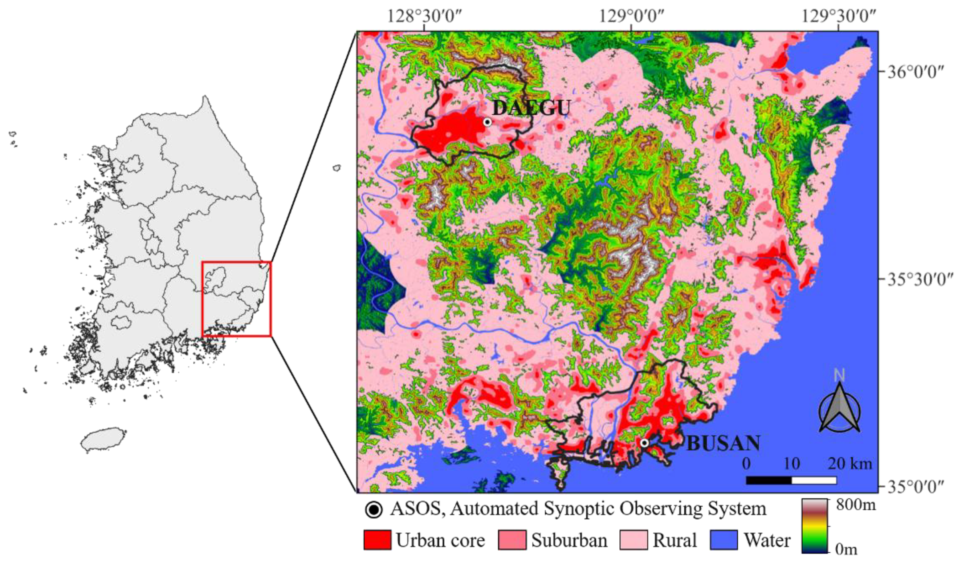
Figure 2.
Comparison of ECOSTRESS and GK-2A LST data at similar times (KST): (a) ECOSTRESS LST at 10:37, (b) GK-2A LST at 10:30 on 9 June 2022, (c) ECOSTRESS LST at 14:25, and (d) GK-2A LST at 14:30 on June 1, 2020.
Figure 2.
Comparison of ECOSTRESS and GK-2A LST data at similar times (KST): (a) ECOSTRESS LST at 10:37, (b) GK-2A LST at 10:30 on 9 June 2022, (c) ECOSTRESS LST at 14:25, and (d) GK-2A LST at 14:30 on June 1, 2020.
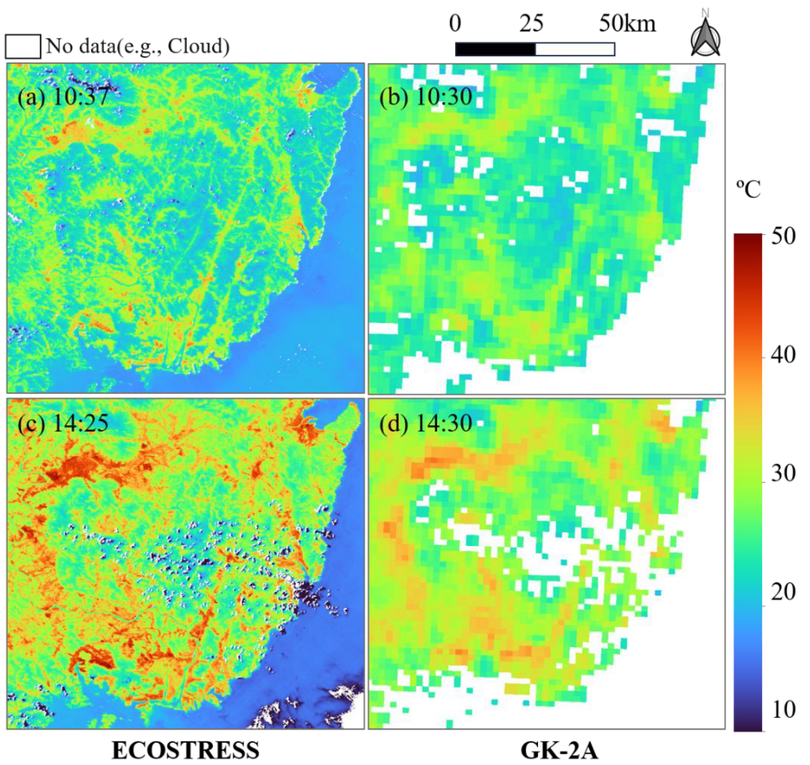
Figure 3.
Scatter plots of ECOSTRESS and GK-2A LST data for 3 urban-scale area types: (a) urban core, (b) suburban, (c) rural, and (d) all area types.
Figure 3.
Scatter plots of ECOSTRESS and GK-2A LST data for 3 urban-scale area types: (a) urban core, (b) suburban, (c) rural, and (d) all area types.
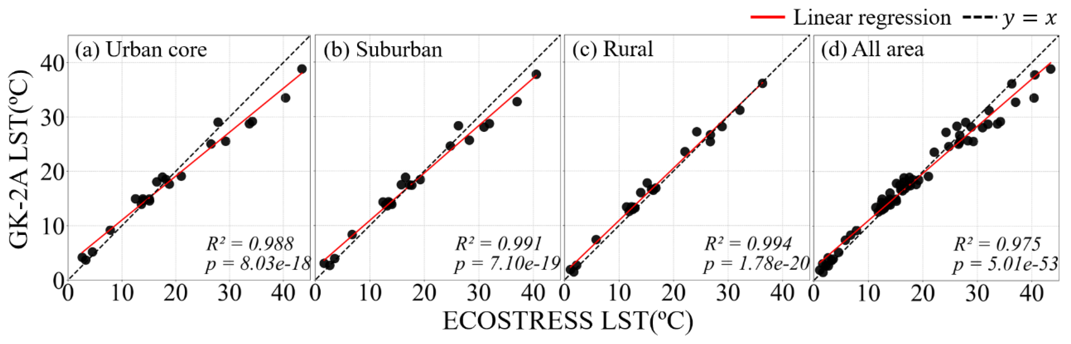
Figure 4.
Land use map of Busan and Daegu. Major industrial complexes were marked (a): NS for Noksan, SC for Science Park, SA for Sasang, and SH for Shinphyung, (b): SS for Seongseo, SD for Seodaegu, TP for third industrial park, and GD for Geomdan.
Figure 4.
Land use map of Busan and Daegu. Major industrial complexes were marked (a): NS for Noksan, SC for Science Park, SA for Sasang, and SH for Shinphyung, (b): SS for Seongseo, SD for Seodaegu, TP for third industrial park, and GD for Geomdan.
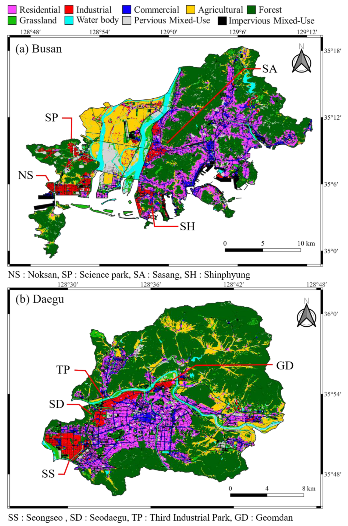
Figure 5.
Histograms of day-to-day LST differences (a) before the daily adjustment, and (b) after the adjustment. The LST differences are calculated from two ECOSTRESS LST scenes, acquired on Oct. 12 and Oct. 30 in 2022, respectively.
Figure 5.
Histograms of day-to-day LST differences (a) before the daily adjustment, and (b) after the adjustment. The LST differences are calculated from two ECOSTRESS LST scenes, acquired on Oct. 12 and Oct. 30 in 2022, respectively.
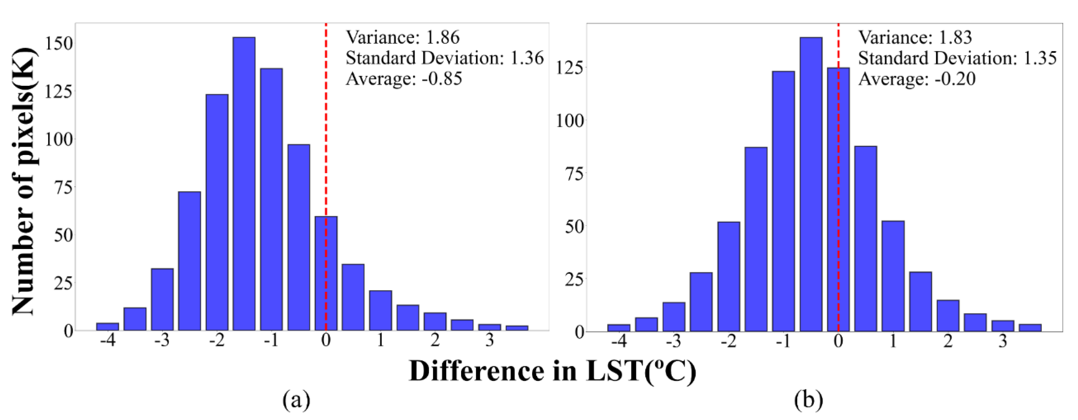
Figure 6.
Diurnal SUHII variation by season of Busan and Daegu in urban-scale. The data were derived from adjusted ECOSTRESS LST and seasonal mean GK-2A LST data for 2020–2022.
Figure 6.
Diurnal SUHII variation by season of Busan and Daegu in urban-scale. The data were derived from adjusted ECOSTRESS LST and seasonal mean GK-2A LST data for 2020–2022.
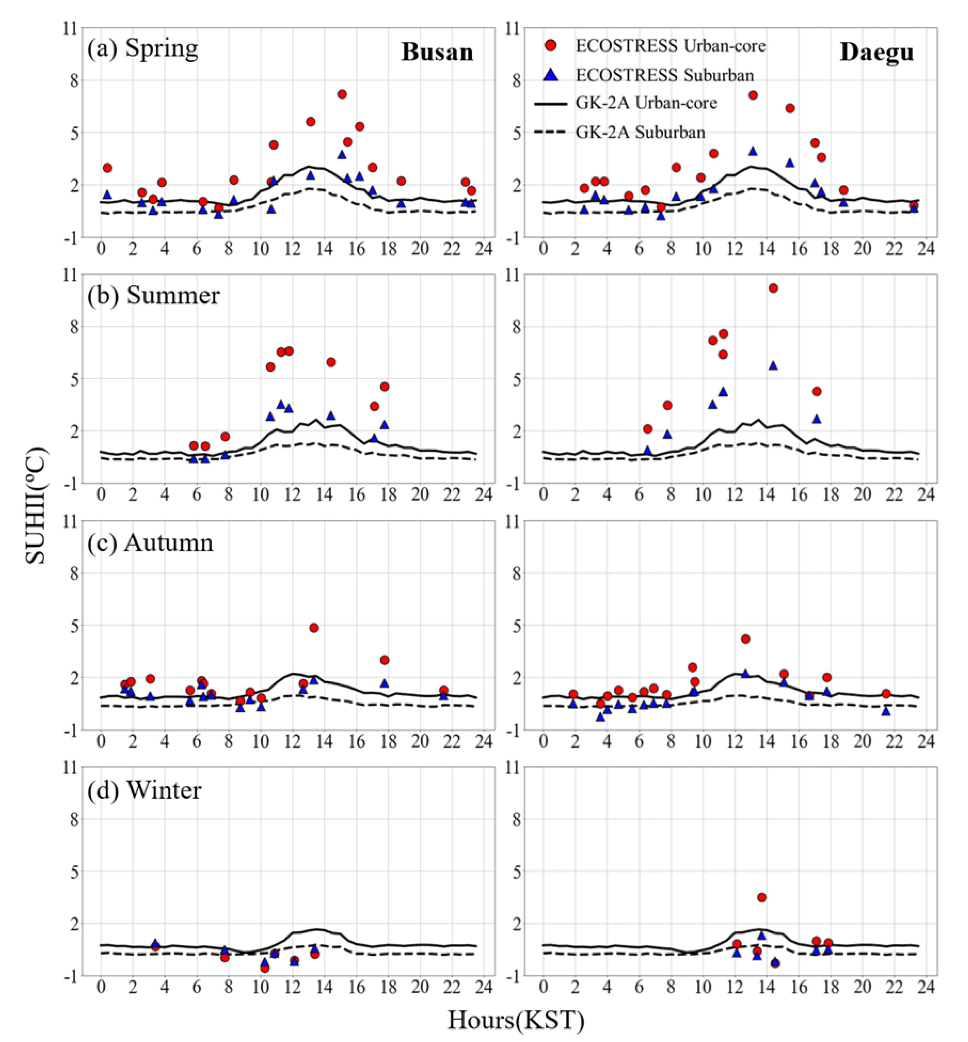
Figure 7.
Season-representative diurnal variation of LST by land use type for Busan and Daegu. The black dotted line represents the diurnal variation of the city-wide average LST derived from GK-2A.
Figure 7.
Season-representative diurnal variation of LST by land use type for Busan and Daegu. The black dotted line represents the diurnal variation of the city-wide average LST derived from GK-2A.
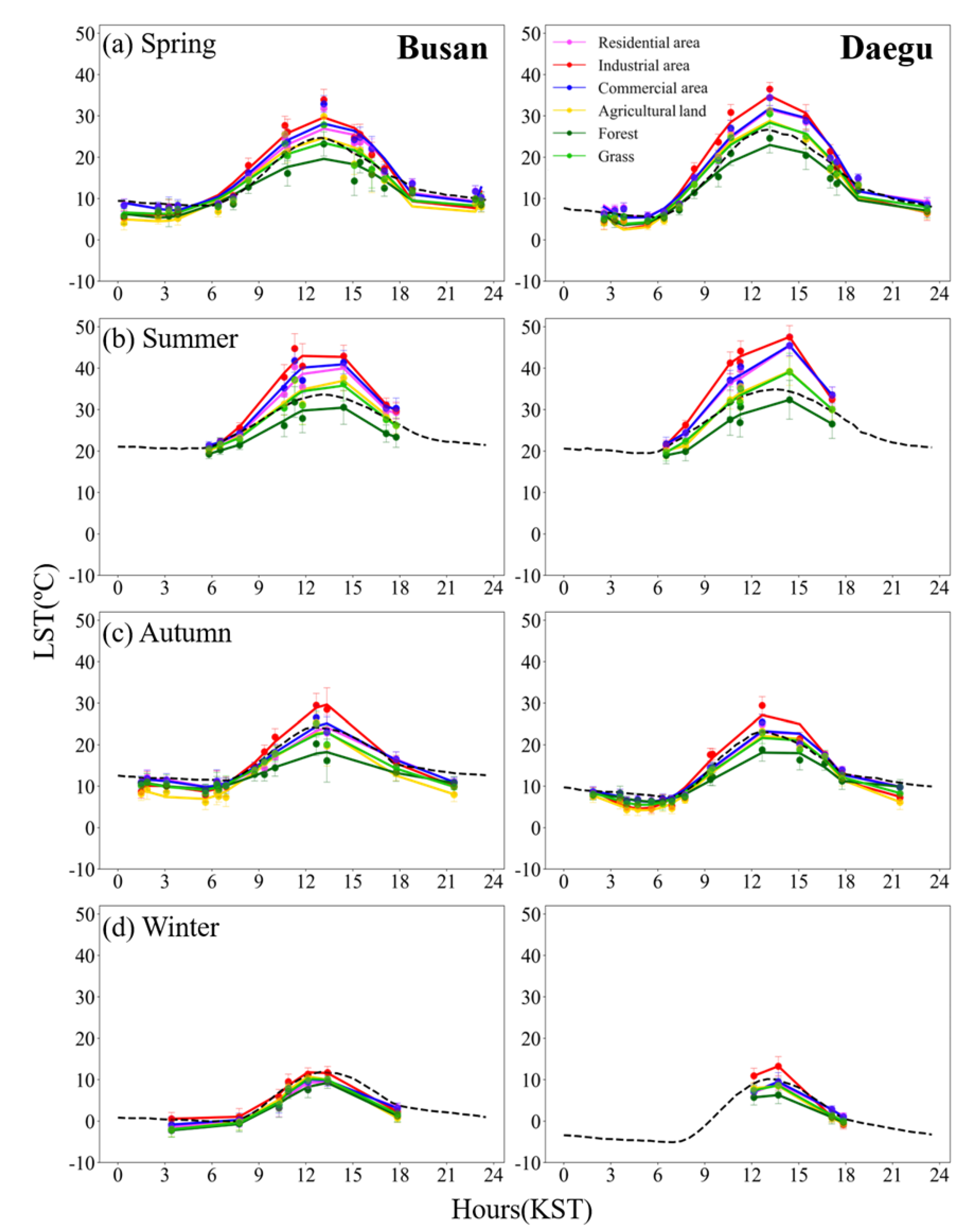
Figure 8.
Diurnal LHI distribution maps for Busan in summer.
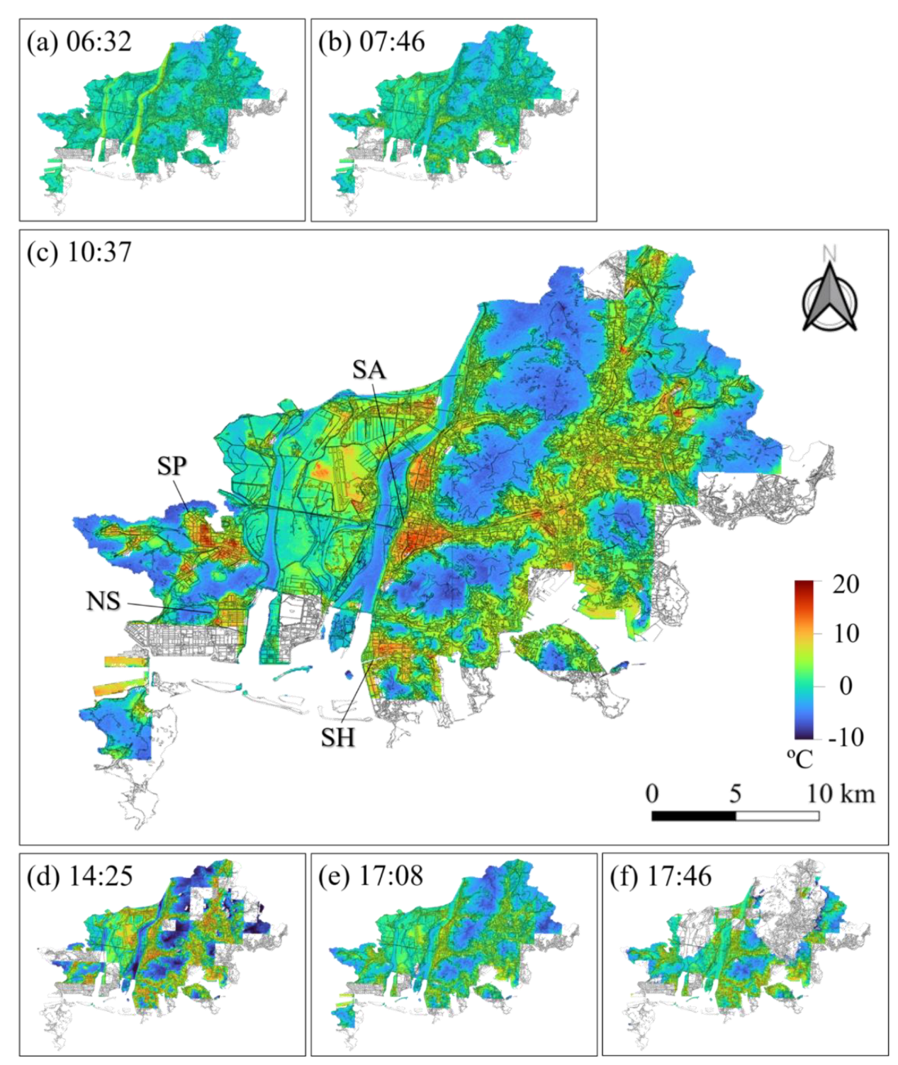
Figure 9.
Diurnal LHI distribution maps for Daegu in summer.
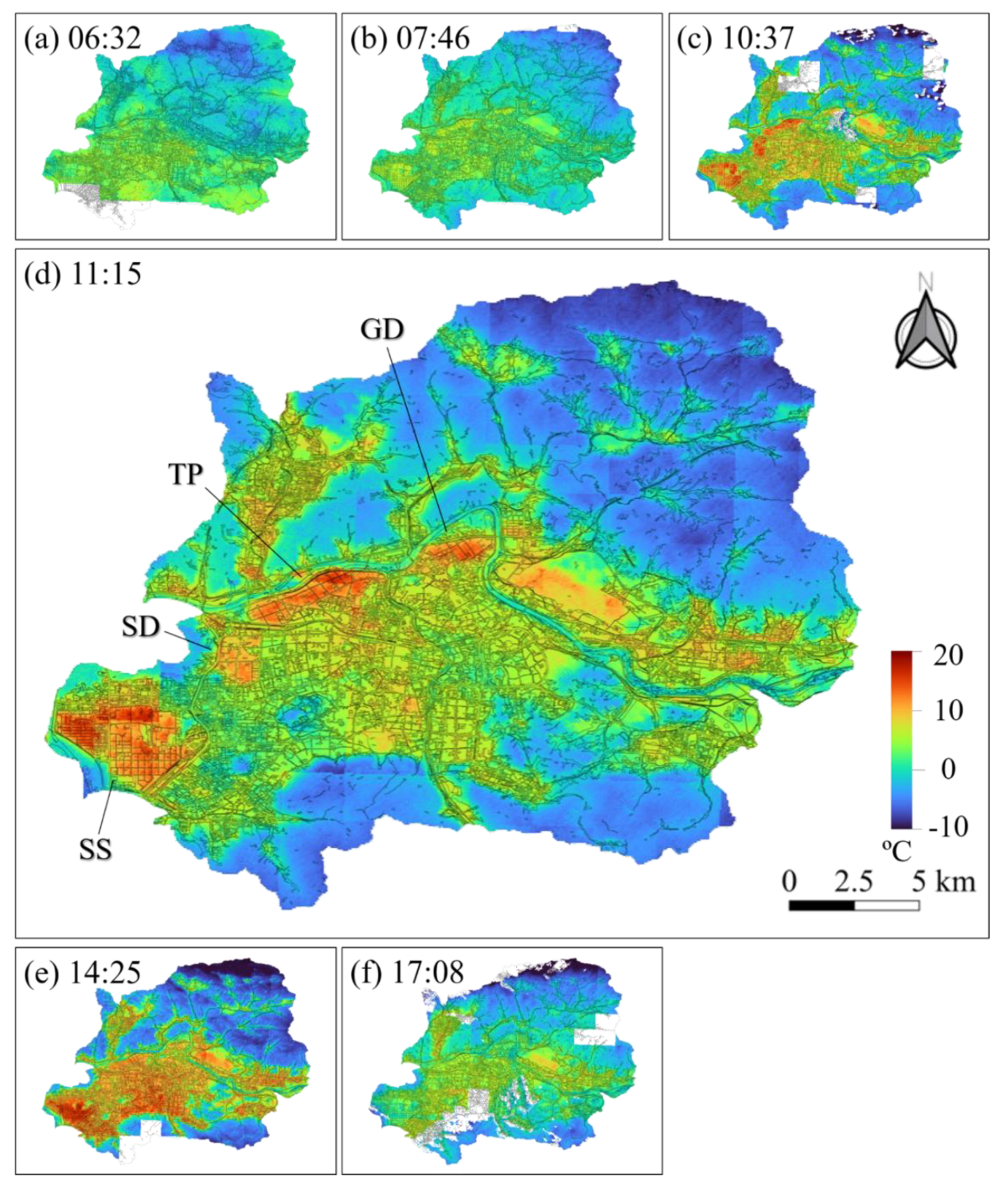
Figure 10.
Dependency of the LHI on the density of residential, industrial, and commercial areas for Busan.
Figure 10.
Dependency of the LHI on the density of residential, industrial, and commercial areas for Busan.
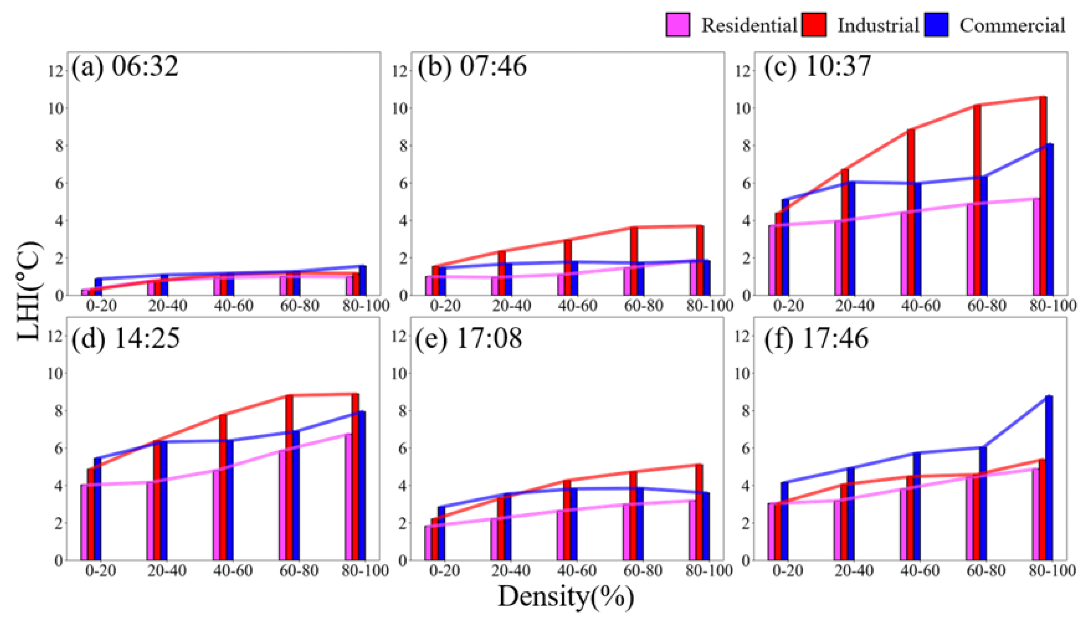
Figure 11.
Dependency of the LHI on the density of residential, industrial, and commercial areas for Daegu.
Figure 11.
Dependency of the LHI on the density of residential, industrial, and commercial areas for Daegu.
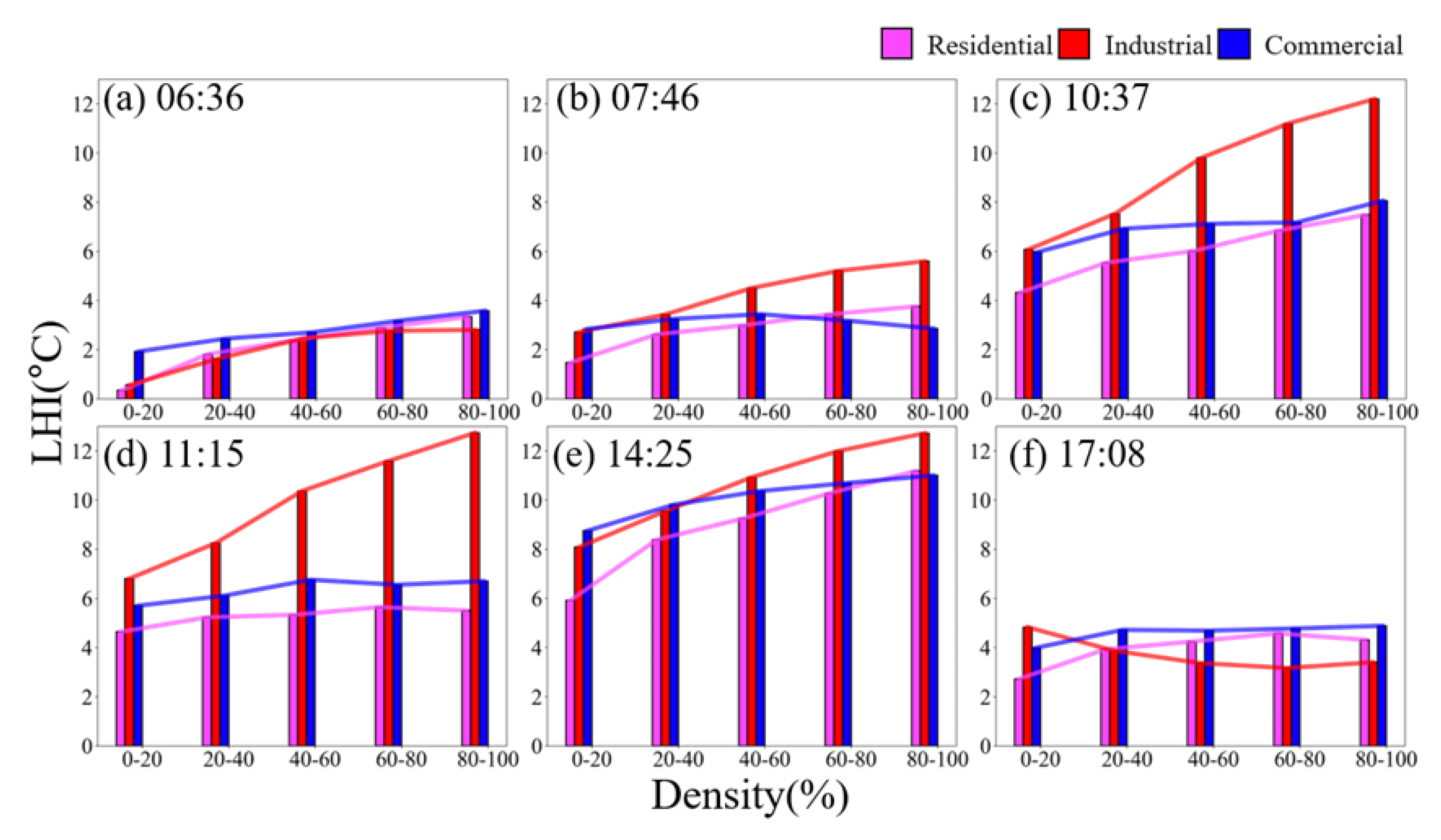
Table 1.
List of land-use types used in this study.
| Level | Hight-level | Middle-level |
| Types | Built Area | Residential Area |
| Industrial Area | ||
| Commercial Area | ||
| Agricultural Land | ||
| Forest | ||
| Grass | ||
Table 2.
Land-use-specific seasonal LST data estimated from ECOSTRESS and GK-2A for 14:25 (KST) in summer.
Table 2.
Land-use-specific seasonal LST data estimated from ECOSTRESS and GK-2A for 14:25 (KST) in summer.
| Land use types | LST (℃) | |||||
| Busan | Daegu | |||||
| ECO | GK2A | Diff | ECO | GK2A | Diff | |
| Residential Area | 40.36 | 33.03 | 7.33 | 45.08 | 36.41 | 8.66 |
| Industrial Area | 42.55 | 33.44 | 9.1 | 47.3 | 39.15 | 8.15 |
| Commercial Area | 41.35 | 33.21 | 8.15 | 45.37 | 36.92 | 8.46 |
| Agricultural Area | 37.63 | 33.97 | 3.66 | 38.66 | 34.08 | 4.58 |
| Forest | 30.97 | 31.77 | -0.8 | 32.71 | 32.47 | 0.24 |
| Grass | 37.18 | 33.1 | 4.07 | 40.32 | 35.51 | 4.81 |
Disclaimer/Publisher’s Note: The statements, opinions and data contained in all publications are solely those of the individual author(s) and contributor(s) and not of MDPI and/or the editor(s). MDPI and/or the editor(s) disclaim responsibility for any injury to people or property resulting from any ideas, methods, instructions or products referred to in the content. |
© 2025 by the authors. Licensee MDPI, Basel, Switzerland. This article is an open access article distributed under the terms and conditions of the Creative Commons Attribution (CC BY) license (http://creativecommons.org/licenses/by/4.0/).
Copyright: This open access article is published under a Creative Commons CC BY 4.0 license, which permit the free download, distribution, and reuse, provided that the author and preprint are cited in any reuse.


