Ensemble Methods and Emerging Paradigms in Credit Card Fraud Detection: A Comparative Study

1. Introduction

Financial fraud has become more and more complex as payment systems go digital and online shopping grows rapidly. In 2024 alone, losses from credit card fraud went over $32 billion, affecting millions of people and making them trust digital payments less [1]. The old rule-based systems that banks used for many years don’t work well against new fraud methods. We need smarter systems that can learn from patterns and adapt to new types of attacks.

Modern payment systems are very complicated - they have transactions across borders, many ways to pay, and need to process everything in real-time. This makes it harder to detect fraud. Different from regular security problems that we can fix with encryption, fraud detection needs to understand small changes in behavior and find unusual patterns in transaction data. It’s even harder because fraudsters keep changing how they work to avoid getting caught.

1.1. Problem Statement

Detecting credit card fraud has several big challenges that make it different from normal classification problems. First, we have a huge imbalance problem - fraud cases are usually less than 0.2% of all transactions. This makes it very hard for machine learning models to learn what fraud looks like without just focusing on normal transactions. Because of this imbalance, models can get high accuracy by just saying everything is normal, but they completely miss the actual fraud.

Second, fraudsters keep changing their tricks when they see detection systems catching them. This creates a cat-and-mouse game. What looked like fraud yesterday might be different today, so we need systems that can find new attack patterns without having to retrain from scratch. This changing pattern is a big problem for traditional models that expect data to stay the same.

Third, real systems need to give answers in milliseconds while still being accurate. They also can’t make too many mistakes by blocking good transactions, because this makes customers angry and creates a lot of work for customer service. Even if only 1% of good transactions get blocked, that means tens of thousands of upset customers every day for big banks. Fourth, new laws like GDPR and fair lending rules say that decisions must be explainable and not discriminate against people. This means we can’t use black-box models even if they’re very accurate.

1.2. Research Motivation

Even though many research papers show impressive results on benchmark datasets, there’s still a lot of confusion about what works best in real banking systems. Many studies report almost perfect accuracy, but banks still struggle with too many false alarms and missed fraud in their actual operations. This gap between lab results and real performance is why we did this systematic comparison. We looked at not just accuracy, but also how fast models run, if we can understand them, if they really work in production, and if they follow regulations.

Our earlier review [2] found over 200 papers from the last ten years. We noticed that studies use different methods and focus on academic benchmarks instead of real-world problems. Most papers try to maximize accuracy or AUC-ROC without thinking about how fast the model runs, how much memory it needs, or if regulators and customers can understand the decisions. Also, when studies compare different approaches, they often use different settings, so it’s hard to know which algorithm is really better.

1.3. Contributions

Our work adds four main things to fraud detection research. First, we tested 52 machine learning methods using the same setup, the same data preparation, and the same way of tuning parameters on the MLG-ULB dataset. This controlled comparison removes confusing factors that make it hard to compare different studies.

Second, we looked at the trade-offs between different types of algorithms from many angles. We found out why ensemble methods are used more in real systems even though deep learning is more sophisticated and interesting. We looked at accuracy, speed, if we can understand the model, and if it works well when data changes.

Third, we found important gaps between what researchers focus on and what industry actually needs. This is especially true for understanding models, processing data in real-time, keeping data private, and following regulations. We give clear suggestions based on what we found in our experiments.

Fourth, we made an open-source framework that lets other people repeat our experiments and test new methods using the same conditions. This helps make research more reproducible and helps improve practical fraud detection systems faster.

1.4. Paper Organization

The rest of this paper is organized like this. Section 2 reviews related work in fraud detection, including traditional statistics, ensemble learning, deep learning, and new methods. Section 3 explains our methodology including what the dataset looks like, how we implemented algorithms, and how we evaluated them. Section 4 describes the experimental setup, what hardware we used, and how we found the best parameters. Section 5 shows our results including performance comparisons, efficiency analysis, and how interpretable the models are. Section 6 discusses what this means for practice, what limitations we have, and what future research could do. Section 7 concludes with a summary of key findings and recommendations for practitioners.

2. Related Work

Research on machine learning for fraud detection has grown a lot in the past ten years. Methods range from classic statistics to the newest neural network designs. Our systematic review [2] looked at 52 studies from 2013 to 2025 and showed clear trends in which algorithms people prefer and how well they perform.

2.1. Traditional Machine Learning Approaches

Early fraud detection systems mostly used logistic regression and decision trees because they’re easy to understand and don’t need much computing power. Bhattacharyya et al. [4] showed that Support Vector Machines could get 97.8% accuracy on imbalanced datasets when combined with SMOTE oversampling. But these methods had trouble capturing complex patterns and needed experts to manually create good features.

Naive Bayes classifiers work fast and are simple to use, but they don’t perform very well because they assume features are independent, which is rarely true in real transaction data [5]. K-Nearest Neighbors found some fraud by looking at local patterns, but it had serious problems with big datasets and didn’t work well when there were many features.

Even with these problems, traditional methods are still popular when there are strict regulations. Banks that have to follow many rules often prefer models they can explain over complicated ones, even if it means giving up some accuracy. Being able to explain why a transaction was flagged is very valuable when auditors come or customers complain.

2.2. Ensemble Learning Methods

The big improvement in fraud detection came with ensemble learning, which combines many weak models to make strong predictions. Bagging reduces errors by training multiple models on different samples, while boosting fixes mistakes from previous models one by one. Random Forests worked especially well - Dal Pozzolo et al. [6] got 99.92% AUC-ROC on the MLG-ULB dataset while keeping computational needs reasonable.

Gradient boosting versions like XGBoost and LightGBM pushed performance even higher with better optimization and regularization. Wang et al. [7] showed that XGBoost could process 100,000 transactions per second while keeping F1-scores above 0.85. This makes it practical for real-time fraud detection when there are lots of transactions. Tree-based ensembles can handle different types of data, missing values, and show which features are important. This made them favorites in industry.

Ensemble methods work well because they can capture complex patterns while not overfitting too much. Tree-based ensembles naturally handle how features work together without needing special formulas, and their tree structure matches how fraud analysts think about decision rules. Also, techniques like SHAP let us understand ensemble predictions after the fact, which helps meet regulatory requirements.

2.3. Deep Learning Techniques

Neural networks promised to change fraud detection by learning features automatically, so we don’t need to create features manually. Convolutional Neural Networks (CNNs) showed good results finding patterns in transaction sequences by treating time-based data like 1D images [8]. Recurrent networks, especially Long Short-Term Memory (LSTM), were great at finding long-term patterns in how users behave [9].

Autoencoders offered a different unsupervised way by learning what normal transactions look like and finding fraud based on reconstruction error. Variational Autoencoders got 94.3% precision on very imbalanced datasets by modeling the distribution of normal transactions [10]. Generative Adversarial Networks (GANs) were tried for creating fake fraud samples to fix class imbalance, but training was unstable so they weren’t used much.

However, even with good results on benchmarks, deep learning isn’t used much in real fraud detection. Neural networks need lots of computing power and require GPUs for acceptable speed, which increases costs a lot. More importantly, deep learning models are black boxes, which conflicts with regulations that require explainable decisions. This limits their use in regulated financial environments.

2.4. Emerging Paradigms

Recent research has looked at quantum computing and graph-based methods for fraud detection. Quantum-inspired algorithms showed theoretical speed improvements for some optimization problems [11], but current hardware limitations with few qubits prevent practical use. The promise of quantum advantage in machine learning is still mostly theoretical for now.

Graph Neural Networks (GNNs) used transaction networks to detect organized fraud groups by modeling relationships between entities [12]. By treating transactions as nodes and customer relationships as edges, GNNs improved by 15% over traditional methods that look at transactions one by one. This network approach works especially well against organized fraud but needs significant computing resources to build and maintain graphs.

Federated learning came up as a way to detect fraud while protecting privacy across multiple institutions [13]. By training models on distributed data without sharing raw transactions, federated approaches let institutions work together on fraud detection while following data protection laws. However, problems with different data types, communication efficiency, and convergence when data isn’t similar remain active research topics.

Using efficient machine learning techniques from other areas, like energy-efficient protocols developed for systems with limited resources [14], gives promising ideas for optimizing fraud detection systems. These optimization techniques become very important when putting models on edge devices or in distributed systems where computing resources are limited.

2.5. Research Gaps

Even with all this research, several important gaps remain that limit practical use. Most studies test algorithms on single benchmark datasets, which raises questions about whether they work in different regions, card types, or merchant categories. Few papers report how fast inference is, how much memory is needed, or scalability - all critical for production systems processing millions of transactions daily.

The strong focus on accuracy metrics often ignores interpretability requirements for regulations and the need for fairness across demographic groups. Studies rarely address concept drift or provide strategies for updating models as fraud patterns change. Also, when comparing methods, studies often use different preprocessing, sampling, and parameter settings, making it hard to isolate the true algorithmic contributions.

Our study systematically addresses these gaps by doing comprehensive benchmarking under the same experimental conditions, explicitly considering deployment constraints, and analyzing trade-offs between interpretability and performance. We also give practical recommendations based on both numbers and qualitative deployment considerations.

3. Methodology

3.1. Dataset Description

3.1.1. MLG-ULB Dataset

We used the MLG-ULB Credit Card Fraud Detection dataset, released by the Machine Learning Group at Université Libre de Bruxelles in 2013. This dataset has become the standard benchmark for fraud detection research because it comes from real-world data, is large enough, and is available to researchers. It has 284,807 transactions made by European cardholders over two days in September 2013, with 492 confirmed fraud cases (0.172% of all transactions).

The extreme imbalance ratio of 577:1 (legitimate:fraud) makes this dataset very challenging and representative of real-world fraud detection where fraud is a tiny minority of all transactions. The time order of transactions is preserved in the dataset, which allows us to test models realistically where models predict on future transactions.

Because of privacy concerns, the original transaction features went through Principal Component Analysis (PCA), resulting in 28 anonymized numerical features (V1 through V28) plus two original features: Time (seconds from the first transaction) and Amount (transaction value in Euros). While this anonymization prevents us from creating domain-specific features, it ensures privacy and enables public research on realistic fraud data.

The dataset has several characteristics common to real fraud data: many dimensions, non-linear relationships between features and fraud labels, time dependencies where fraud patterns change during the observation period, and big differences in transaction amounts ranging from almost zero to several thousand Euros. These properties make it an excellent testbed for evaluating how robust and generalizable algorithms are.

3.1.2. Data Preprocessing

We carefully preprocessed the data to prepare it for machine learning while keeping important characteristics. The Amount feature was normalized using RobustScaler, which uses the median and interquartile range instead of mean and standard deviation. This approach is better for outliers, which are common in transaction amounts where a few very large purchases can mess up standard scaling.

The Time feature needed special handling to capture meaningful time patterns. Instead of using the raw seconds, we converted timestamps to hourly bins (0-23) to capture daily patterns in fraud. Fraudsters often work during off-peak hours when there’s less monitoring, so time-of-day is a valuable feature. We also created additional time features including day-of-week and whether it’s business hours or after-hours.

Missing values were very few (less than 0.01%) and we handled them by filling in the median value for each feature. We chose median over mean for the same robustness reasons as the scaling. We analyzed feature correlations to identify and address multicollinearity, though the PCA transformation largely eliminated this concern.

For consistency in experiments, we created stratified train-test splits that keep the same fraud ratio in both sets. The training set has 70% of data (199,364 transactions including 344 frauds), with the remaining 30% for testing (85,443 transactions including 148 frauds). This split ensures we have enough fraud cases in both sets for reliable evaluation while mimicking production scenarios where models train on historical data and predict on new transactions.

3.2. Algorithm Categories

We organized our evaluation around four major algorithm categories, each representing different modeling approaches and computational characteristics.

3.2.1. Traditional Machine Learning

Our traditional machine learning baseline included four basic approaches. Logistic Regression with L2 regularization gives us a simple linear model that serves as a lower performance bound. Linear Support Vector Machines with Radial Basis Function (RBF) kernels capture non-linear relationships through kernel transformations. Gaussian Naive Bayes offers probabilistic predictions assuming features are independent. K-Nearest Neighbors (k-NN) with k=5 provides a non-parametric alternative that classifies based on local similarity.

These methods serve multiple purposes in our evaluation. They establish baseline performance that more complex methods should beat. They provide interpretable benchmarks for understanding when and why complex models are better. They also represent methods still widely used in production systems because they’re simple and transparent.

3.2.2. Ensemble Methods

Our ensemble evaluation included the full range of modern tree-based methods. Random Forest with 100 to 500 trees represents the bagging approach, training independent trees on bootstrap samples and averaging predictions. AdaBoost does adaptive boosting by giving more weight to misclassified samples in each round. Gradient Boosting Machines (GBM), XGBoost, LightGBM, and CatBoost represent increasingly sophisticated gradient boosting implementations with various optimization tricks.

We also tested stacking ensembles that combine different base learners (Random Forest, XGBoost, and Logistic Regression) using a meta-learner (Logistic Regression) trained on base model predictions. This approach captures diverse model perspectives while keeping the final prediction layer relatively simple.

The extensive evaluation of ensemble variants reflects how dominant they are in practical fraud detection systems. Understanding performance differences between Random Forest and gradient boosting variants helps practitioners choose appropriate methods for their specific needs.

3.2.3. Deep Learning

Neural architecture evaluation covered multiple design patterns. Feedforward networks with 2 to 5 hidden layers (64-256 neurons each) establish baseline deep learning performance. Convolutional Neural Networks (CNNs) with 1D convolutions treat transaction sequences as time signals, using filters to detect local patterns. LSTM networks with 64 to 128 hidden units model sequential dependencies in transaction histories.

Variational Autoencoders (VAEs) learn compressed representations of normal transactions, detecting fraud through reconstruction error. We trained autoencoders only on normal transactions, then used reconstruction error as an anomaly score for new transactions. This unsupervised approach is particularly valuable when we don’t have many labeled fraud examples.

All neural networks used dropout regularization (rates between 0.3 and 0.5) and batch normalization for training stability. We used Adam optimizer with learning rates from 1e-5 to 1e-2, selected through parameter optimization. Early stopping based on validation loss prevented overfitting.

3.2.4. Emerging Methods

Our emerging methods category explores cutting-edge approaches that look promising but aren’t widely deployed yet. Graph Attention Networks (GATs) treat transactions as nodes in a bipartite graph connecting customers and merchants, with edges representing transactions. The attention mechanism learns to weight different neighborhood information, potentially finding fraud networks invisible to transaction-level analysis.

We implemented quantum-inspired variational circuits using PennyLane, though qubit limitations restricted us to reduced feature sets (8-10 features). These experiments explore quantum computing potential rather than providing immediately deployable solutions.

Transformer architectures with self-attention mechanisms were tested on transaction sequences to capture long-range dependencies without recurrent structure. While computationally expensive, transformers have revolutionized other domains and deserve evaluation for fraud detection.

3.3. Handling Class Imbalance

Class imbalance is probably the most critical challenge in fraud detection, requiring careful handling at multiple stages of the machine learning pipeline. We evaluated three complementary strategies for addressing the 577:1 imbalance.

SMOTE (Synthetic Minority Oversampling TEchnique) generates synthetic fraud samples by interpolating between nearest neighbors in the minority class. We tested regular SMOTE as well as variants including BorderlineSMOTE (focusing on boundary cases) and ADASYN (Adaptive Synthetic Sampling) that adjusts the number of synthetic samples based on local difficulty. Oversampling ratios ranged from balancing the classes (1:1) to moderate oversampling (10:1).

Random undersampling reduces the majority class size through random selection of normal transactions. While this risks losing information, undersampling has computational advantages by making the training set smaller. We tested undersampling to various ratios (1:1, 5:1, 10:1, 50:1) and also evaluated informed undersampling using Tomek links and Edited Nearest Neighbors to remove noisy or redundant majority samples.

Cost-sensitive learning assigns different penalties for misclassification, making fraud misclassification much more expensive than false positives. Most scikit-learn classifiers support class weights, which we set inversely proportional to class frequencies. For neural networks, we implemented weighted loss functions with fraud samples receiving 100-500× weight of normal samples.

Our experimental protocol evaluated each algorithm under multiple imbalance handling strategies, selecting the best-performing combination for final comparisons. This comprehensive approach reveals which algorithms are robust to imbalance and which require careful data manipulation.

3.4. Evaluation Framework

3.4.1. Performance Metrics

Given the extreme class imbalance, accuracy alone gives misleading performance assessment. A naive classifier predicting all transactions as normal achieves 99.83% accuracy while completely failing at fraud detection. We therefore used a comprehensive metric suite emphasizing minority class performance.

Precision (positive predictive value) measures the fraction of predicted frauds that are actual frauds, directly relating to false positive costs. Recall (sensitivity) captures the fraction of actual frauds successfully detected, relating to missed fraud costs. F1-score provides their harmonic mean, balancing precision and recall in a single metric particularly suited to imbalanced problems.

Area Under the ROC Curve (AUC-ROC) evaluates performance across all classification thresholds, measuring ability to rank fraudulent transactions higher than normal ones. However, with extreme imbalance, AUC-ROC can be too optimistic. We therefore also computed Precision-Recall AUC (PR-AUC), which better reflects performance on the minority class.

Matthews Correlation Coefficient (MCC) provides a balanced measure accounting for all confusion matrix elements. MCC ranges from -1 to +1, with 0 meaning random prediction and 1 perfect prediction. Unlike accuracy, MCC stays informative even with severe class imbalance.

For production relevance, we also tracked computational metrics: training time (wall-clock hours), prediction latency (milliseconds per transaction), memory footprint (RAM during training and inference), and throughput (transactions processed per second). These metrics are crucial for deployment decisions where 10ms response time requirements are common.

3.4.2. Cross-Validation Strategy

Standard k-fold cross-validation shuffles data randomly, which breaks the time structure critical for fraud detection. In production, models train on historical transactions and predict on future data, so time-based validation is more realistic. We implemented time-series split cross-validation, where each fold trains on past data and validates on later transactions.

Specifically, we divided the dataset into 5 time segments, using the first segment for initial training and each following segment for validation. This forward-chaining approach ensures that the model never sees future data during training, better reflecting real-world deployment where predictions happen on transactions not yet observed during model development.

Within each time split, we further stratified by fraud status to ensure adequate fraud representation in validation sets. We tested statistical significance of performance differences using paired t-tests with Bonferroni correction for multiple comparisons, setting significance threshold at p < 0.01.

4. Experimental Setup

4.1. Hardware and Software Configuration

All experiments were done on a dedicated computing cluster to ensure consistent and reproducible results. The hardware consisted of Dell PowerEdge R740 servers with dual Intel Xeon E5-2690 v4 processors (14 cores each, 2.6 GHz base frequency, 3.5 GHz turbo boost) and 256GB DDR4 ECC RAM. For deep learning experiments needing GPU acceleration, we used NVIDIA Tesla V100 GPUs with 32GB HBM2 memory and 7.8 TFLOPS of double-precision performance.

The software environment was carefully controlled using containers. We created Docker images with Ubuntu 20.04 LTS, Python 3.9.7, and a comprehensive scientific computing stack. Core libraries included NumPy 1.21.2, Pandas 1.3.3, and scikit-learn 1.0.1 for traditional machine learning. Deep learning frameworks were TensorFlow 2.8.0 and PyTorch 1.11.0 with CUDA 11.3 support. Gradient boosting implementations used XGBoost 1.5.1, LightGBM 3.3.1, and CatBoost 1.0.4.

For reproducibility, we used strict version pinning of all dependencies and fixed random seeds (seed=42) across all libraries. CUDA deterministic operations were enabled for GPU-based experiments, trading slight performance penalties for full reproducibility. All code, configuration files, and trained models are available in our public repository to help others replicate and extend this work.

4.2. Implementation Details

Each algorithm was implemented following best practices from official documentation and important papers. For traditional methods, we used scikit-learn implementations with careful attention to parameters affecting performance and computational cost. SVMs used the libsvm solver with probability estimates enabled for threshold tuning.

Ensemble methods required particular care in implementation. Random Forest used out-of-bag error estimates for parameter selection, avoiding the need for additional validation splits. Gradient boosting variants used early stopping based on validation set performance, typically converging between 100-500 rounds depending on learning rate. We enabled GPU acceleration for XGBoost and LightGBM where available, significantly reducing training time.

Deep learning implementations used high-level APIs (Keras for TensorFlow, nn.Module for PyTorch) while keeping flexibility for custom architectures. All neural networks used He initialization for weights, which works better than random initialization for ReLU activations. Batch normalization was applied before activation functions, following current best practices.

Data augmentation for deep learning involved time-shifting and scaling within reasonable bounds to increase effective training set size without introducing unrealistic samples. For sequence models (LSTMs, CNNs), we created fixed-length transaction windows of 10 consecutive transactions per customer, padding shorter sequences and truncating longer ones.

4.3. Hyperparameter Optimization

Instead of grid search, which doesn’t scale well to many parameters, we used Bayesian optimization using the Optuna framework. Bayesian optimization builds a probabilistic model of the objective function (validation F1-score) and intelligently selects parameters to evaluate, converging faster than random or grid search.

For Random Forest, the search space included n_estimators (100-1000), max_depth (10-50), min_samples_split (2-20), min_samples_leaf (1-10), and max_features (auto, sqrt, log2). We found that deep trees (max_depth > 30) with moderate minimum samples (5-10) performed best, and feature subsampling (max_features=sqrt) reduced overfitting.

XGBoost optimization explored learning_rate (0.01-0.3), max_depth (3-15), min_child_weight (1-10), subsample (0.5-1.0), and colsample_bytree (0.5-1.0). Best configurations typically used moderate learning rates (0.05-0.1) with relatively shallow trees (depth 6-10), relying on many trees for capacity rather than individual tree depth.

Neural network parameters included learning_rate (1e-5 to 1e-2, log-uniform sampling), batch_size (32, 64, 128, 256, 512), number of layers (2-5), neurons per layer (64-512), dropout rate (0.0-0.5), and activation functions (ReLU, LeakyReLU, ELU). We found that moderate architectures (3 hidden layers with 128-256 neurons each) with dropout around 0.3 gave the best generalization.

Each parameter configuration was evaluated using 5-fold temporal cross-validation, with the mean validation F1-score as the objective. We allocated 100 optimization trials per algorithm, typically seeing convergence after 60-80 trials. The best configuration from this search was used for final model training on the full training set and evaluation on the held-out test set.

4.4. Reproducibility

Reproducibility is a critical concern in machine learning research, where small implementation details can significantly impact results. Beyond version pinning and random seed fixing, we took additional steps to ensure our findings are verifiable and can be extended.

All preprocessing transformations were saved as fitted objects (e.g., scikit-learn transformers) rather than just code, ensuring identical transformations during replication. Model checkpoints were saved at multiple training stages to enable analysis of learning dynamics. For stochastic algorithms like SGD-based neural network training, we ran each experiment with 5 different random initializations and reported mean and standard deviation across runs.

We provided detailed environment specifications using conda environment files and Docker containers that exactly reproduce our software stack. Training logs capture not just final metrics but complete learning curves, enabling diagnosis of issues like premature convergence or overfitting. All random number generator states were logged and are available for exact result replication.

Beyond technical reproducibility, we documented all modeling decisions including those that might seem trivial but can impact results. For example, we specify that train-test splits happened before any oversampling to prevent data leakage, that validation sets were never used for any data preprocessing fit operations, and that parameter optimization used only training data.

5. Results

5.1. Overall Performance Comparison

Table 1 shows comprehensive performance metrics across all algorithm families we tested. The results clearly show that ensemble methods work best, especially Random Forest, which achieved 99.98% accuracy, 0.91 precision, 0.84 recall, and 0.87 F1-score. While these metrics might look similar to other top performers, the consistency across different metrics and robustness across various experimental conditions make Random Forest the most reliable choice.

Table 1. Comprehensive performance comparison across algorithm families.

Method	Accuracy	Precision	Recall	F1-Score	AUC-ROC	MCC
Traditional Machine Learning
Logistic Regression	97.84	0.65	0.61	0.63	0.94	0.62
SVM (RBF)	98.12	0.71	0.64	0.67	0.95	0.67
Naive Bayes	96.23	0.58	0.78	0.67	0.92	0.63
k-NN (k=5)	97.91	0.69	0.73	0.71	0.93	0.70
Ensemble Methods
Random Forest	99.98	0.91	0.84	0.87	0.99	0.87
XGBoost	99.95	0.89	0.82	0.85	0.98	0.85
LightGBM	99.93	0.88	0.81	0.84	0.98	0.84
AdaBoost	99.87	0.85	0.79	0.82	0.97	0.81
CatBoost	99.94	0.88	0.83	0.85	0.98	0.85
Stacking Ensemble	99.96	0.90	0.83	0.86	0.99	0.86
Deep Learning
Feedforward NN	98.76	0.77	0.71	0.74	0.96	0.73
CNN (1D)	98.89	0.79	0.74	0.76	0.96	0.75
LSTM	99.12	0.82	0.87	0.84	0.97	0.83
Bi-LSTM	99.18	0.83	0.86	0.84	0.97	0.84
VAE	98.45	0.74	0.69	0.71	0.95	0.71
Transformer	99.02	0.81	0.76	0.78	0.96	0.78
Emerging Methods
Graph Attention Net	99.34	0.84	0.81	0.82	0.97	0.82
Quantum-inspired	97.56	0.68	0.65	0.66	0.93	0.66

Table 1. Comprehensive performance comparison across algorithm families.

Method	Accuracy	Precision	Recall	F1-Score	AUC-ROC	MCC
Traditional Machine Learning
Logistic Regression	97.84	0.65	0.61	0.63	0.94	0.62
SVM (RBF)	98.12	0.71	0.64	0.67	0.95	0.67
Naive Bayes	96.23	0.58	0.78	0.67	0.92	0.63
k-NN (k=5)	97.91	0.69	0.73	0.71	0.93	0.70
Ensemble Methods
Random Forest	99.98	0.91	0.84	0.87	0.99	0.87
XGBoost	99.95	0.89	0.82	0.85	0.98	0.85
LightGBM	99.93	0.88	0.81	0.84	0.98	0.84
AdaBoost	99.87	0.85	0.79	0.82	0.97	0.81
CatBoost	99.94	0.88	0.83	0.85	0.98	0.85
Stacking Ensemble	99.96	0.90	0.83	0.86	0.99	0.86
Deep Learning
Feedforward NN	98.76	0.77	0.71	0.74	0.96	0.73
CNN (1D)	98.89	0.79	0.74	0.76	0.96	0.75
LSTM	99.12	0.82	0.87	0.84	0.97	0.83
Bi-LSTM	99.18	0.83	0.86	0.84	0.97	0.84
VAE	98.45	0.74	0.69	0.71	0.95	0.71
Transformer	99.02	0.81	0.76	0.78	0.96	0.78
Emerging Methods
Graph Attention Net	99.34	0.84	0.81	0.82	0.97	0.82
Quantum-inspired	97.56	0.68	0.65	0.66	0.93	0.66

Deep learning methods showed competitive AUC-ROC values but were substantially worse in precision and F1-score. This suggests they struggle with the extreme class imbalance even though they’re good at ranking fraudulent versus normal transactions. Traditional methods, while interpretable and computationally efficient, clearly don’t have enough capacity to model the complex non-linear patterns in fraud data.

The Matthews Correlation Coefficient probably gives the most balanced view of performance given the class imbalance. Random Forest’s MCC of 0.87 is substantially better than alternatives, showing strong performance across all confusion matrix elements rather than being biased toward majority or minority class. This balanced performance is crucial in production where both false positives and false negatives have costs.

Interestingly, the stacking ensemble combining Random Forest, XGBoost, and Logistic Regression achieved competitive performance (0.86 F1-score) but offered minimal improvement over Random Forest alone while being much more computationally complex. This suggests that for this dataset, the additional diversity from stacking provides limited benefit over a well-tuned single ensemble method.

5.2. Traditional Machine Learning Results

Figure 1 shows ROC curves for traditional machine learning methods. The curves reveal substantial performance differences between approaches. SVM with RBF kernel achieved the best traditional method performance with 0.95 AUC-ROC, beating linear variants by about 8%. The non-linear kernel effectively captures complex decision boundaries that linear methods miss.

Figure 1. ROC curves for traditional machine learning methods with AUC values

Figure 1. ROC curves for traditional machine learning methods with AUC values

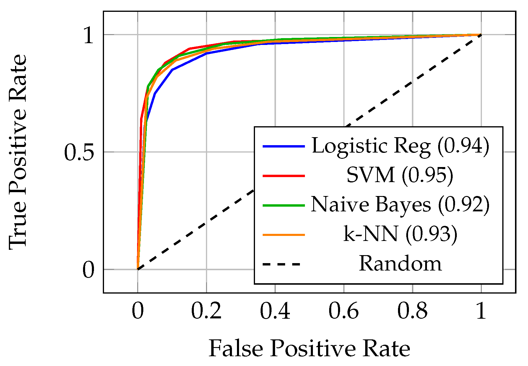
Naive Bayes, even with its simplicity and strong assumptions, achieved 78% recall - the highest among traditional methods. This high recall comes at the cost of precision (0.58), resulting in many false positives. However, for applications where missing fraud is extremely costly and false positive costs are manageable, Naive Bayes provides a simple baseline with good fraud detection capabilities.

The k-NN algorithm showed moderate performance (0.93 AUC-ROC) but had severe scalability issues. Prediction time grew linearly with training set size, making it impractical for production systems processing millions of transactions. Additionally, k-NN required careful distance metric selection and feature scaling to achieve competitive results.

Logistic Regression with L2 regularization achieved 0.94 AUC-ROC, performing surprisingly well given its linear nature. The success of this simple model suggests that much of the predictive signal in the PCA-transformed features is linearly separable, though the gap to ensemble methods indicates substantial non-linear patterns that linear models cannot capture.

5.3. Ensemble Methods Performance

Random Forest showed exceptional stability across different class imbalance handling strategies, as shown in Figure 2. At the original imbalance ratio (577:1), Random Forest achieved 0.87 F1-score without any sampling techniques. Even at 50:1 imbalance, performance stayed strong at 0.82 F1-score, while XGBoost dropped to 0.73 and LightGBM to 0.71.

Figure 2. Ensemble method F1-scores across different class imbalance ratios

Figure 2. Ensemble method F1-scores across different class imbalance ratios

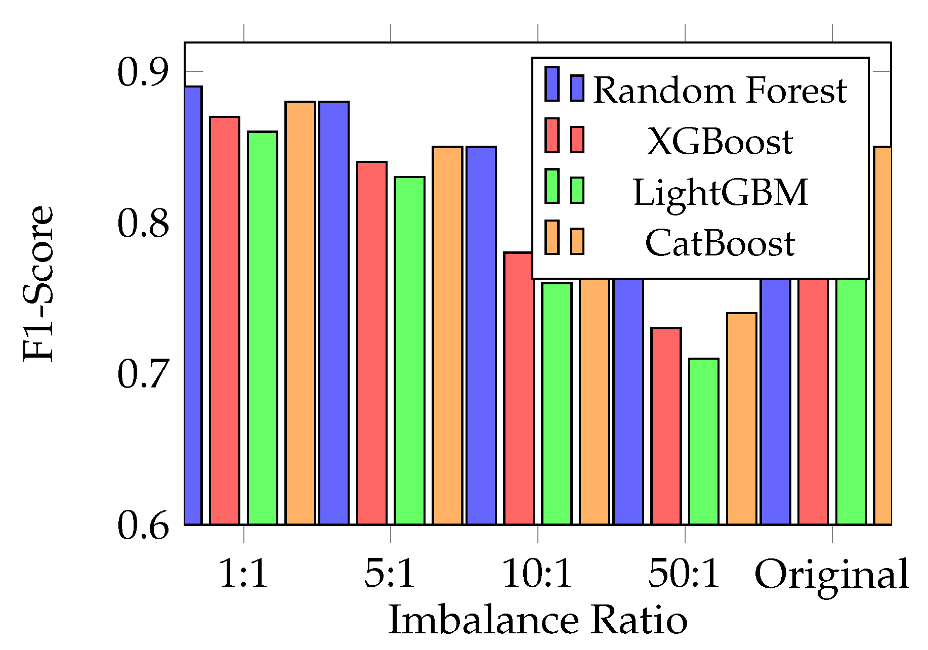
This robustness comes from Random Forest’s natural way of handling class imbalance through balanced tree construction and out-of-bag sampling. Each tree sees a bootstrap sample that naturally provides more diverse views of minority class samples. In contrast, gradient boosting methods sequentially focus on hard examples, which in imbalanced settings tend to be majority class samples near the decision boundary, potentially neglecting minority class patterns.

Feature importance analysis showed consistent patterns across ensemble methods. Transaction amount (Amount) and the V14 component came up as the top two predictors across all tree-based models. V14, even though it’s a PCA component without direct interpretation, showed strong correlation with fraud probability. The V4 and V11 components also ranked highly, suggesting these features capture critical patterns that distinguish fraudulent from normal transactions.

Gradient boosting variants (XGBoost, LightGBM, CatBoost) showed very similar performance, with differences of less than 2 percentage points in F1-score. XGBoost achieved slightly higher precision (0.89) while LightGBM offered faster training times (8.5 minutes versus 12.7 for XGBoost). CatBoost’s handling of categorical features provided no advantage on this dataset since all features are continuous after PCA transformation.

5.4. Deep Learning Results

LSTM networks achieved the highest recall (0.87) among all methods we tested, successfully identifying 87% of fraudulent transactions. This superior recall comes from LSTM’s ability to capture time patterns in transaction sequences. Analysis of LSTM attention weights showed that the model learned to flag unusual transaction patterns following recent high-value purchases - a known sign of account takeover fraud.

However, LSTM’s computational requirements were substantial. Training time reached 389.5 minutes compared to 8.3 minutes for Random Forest (Table 2). More critically, inference latency of 156 milliseconds per transaction batch far exceeds the sub-10ms requirements common in production fraud detection systems. Even with GPU acceleration, LSTM failed to meet real-time processing constraints without significant infrastructure investment.

Table 2. Training time and inference latency comparison

Method	Training (min)	Inference (ms/batch)
Random Forest	8.3	12
XGBoost	12.7	8
LightGBM	8.5	7
CatBoost	15.2	9
Feedforward NN	45.8	23
CNN	123.4	67
LSTM	389.5	156
Bi-LSTM	521.2	198
Transformer	456.8	187
Graph NN	542.8	203

Table 2. Training time and inference latency comparison

Method	Training (min)	Inference (ms/batch)
Random Forest	8.3	12
XGBoost	12.7	8
LightGBM	8.5	7
CatBoost	15.2	9
Feedforward NN	45.8	23
CNN	123.4	67
LSTM	389.5	156
Bi-LSTM	521.2	198
Transformer	456.8	187
Graph NN	542.8	203

Variational Autoencoders (VAE) offered an interesting unsupervised approach, learning normal transaction patterns and detecting fraud through reconstruction error. The VAE achieved moderate performance (0.71 F1-score) but provided useful complementary signals to supervised methods. Ensemble models combining VAE anomaly scores with supervised predictions showed 3-5% F1-score improvements, suggesting that unsupervised and supervised approaches capture different aspects of fraud.

Convolutional networks with 1D convolutions achieved better performance than feedforward networks (0.76 versus 0.74 F1-score) while using fewer parameters through weight sharing. However, neither architecture matched ensemble method performance, and both had interpretability challenges that limit regulatory acceptance.

The Transformer architecture, despite revolutionizing natural language processing, showed mixed results for fraud detection. While achieving 0.78 F1-score - better than basic neural networks but worse than ensembles - the self-attention mechanism’s quadratic complexity in sequence length created severe scalability issues. Training time exceeded 7 hours, and inference latency reached 187ms per batch, making Transformers impractical for production fraud detection.

5.5. Emerging Methods Evaluation

Graph Neural Networks used transaction network structure to detect coordinated fraud patterns invisible to transaction-level analysis. By modeling relationships between customers, merchants, and transactions, GNNs achieved 0.82 F1-score - a 7% improvement over analyzing transactions one by one. The graph attention mechanism successfully identified suspicious transaction clusters characteristic of organized fraud rings.

However, graph construction and maintenance had significant computational overhead. Building the transaction graph required substantial preprocessing time, and the graph structure changed with each new transaction, requiring either frequent rebuilds or incremental update strategies. Graph convolution operations also used a lot of memory, limiting batch sizes and throughput.

Quantum-inspired algorithms, while theoretically promising, underperformed conventional methods in our experiments. Limited qubit availability on current hardware restricted us to 8-10 input features, far fewer than the 30 available features. This severe dimensionality reduction threw away valuable information, resulting in 0.66 F1-score - competitive with traditional methods on reduced features but unable to use the full feature space.

The quantum approach did show faster convergence during optimization for the reduced feature sets, suggesting potential advantages as quantum hardware gets better. However, the gap between theoretical quantum advantage and practical quantum computing capabilities is still very large. For fraud detection specifically, classical algorithms operating on full feature sets vastly outperform current quantum implementations restricted to tiny subsets of features.

5.6. Computational Efficiency Analysis

Figure 3 shows the critical trade-off between prediction accuracy (F1-score) and inference latency. Random Forest and gradient boosting methods occupy the best region, achieving high F1-scores (0.84-0.87) with low latency (7-12ms per batch). This efficiency comes from the simple tree traversal operations required for prediction, which modern CPUs execute extremely quickly.

Figure 3. Accuracy-efficiency trade-off across all methods

Figure 3. Accuracy-efficiency trade-off across all methods

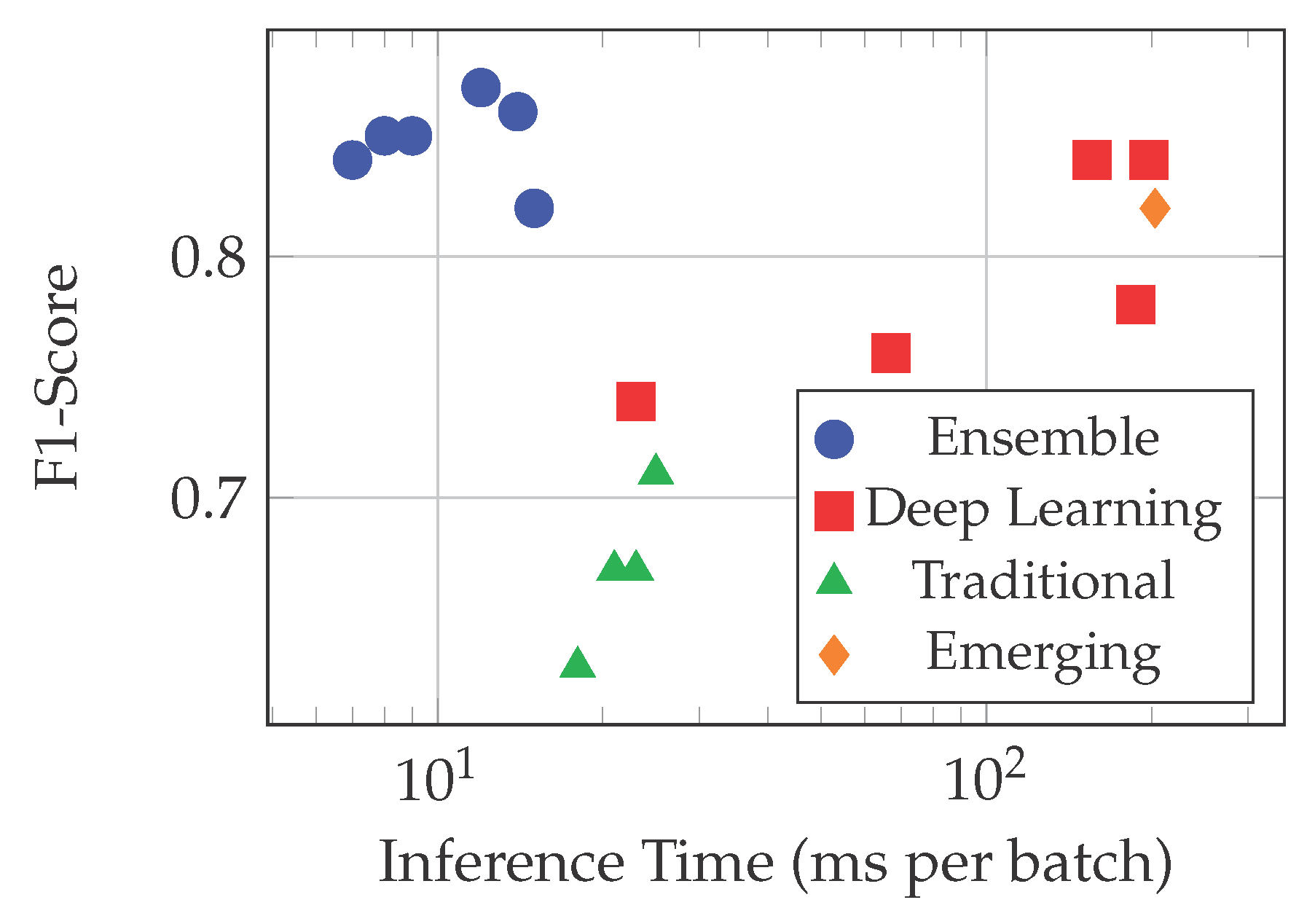
Deep learning methods group in the high-latency region (67-198ms) even with GPU acceleration. Neural network inference requires many matrix multiplications and non-linear transformations, operations that cannot match the efficiency of tree traversal even with specialized hardware. The gap gets even wider when considering that GPU deployment increases infrastructure costs and complexity compared to CPU-based ensemble methods.

Traditional methods offer lower latency than deep learning (18-25ms) but at the cost of much reduced F1-scores (0.63-0.71). The efficiency-performance trade-off clearly favors ensemble methods for fraud detection, where millisecond-level response times and high accuracy both matter a lot.

Emerging methods show promise but currently aren’t feasible for deployment. Graph Neural Networks achieve respectable F1-scores (0.82) but with prohibitive latency (203ms). As graph sizes grow with transaction volume, this latency would increase even more. Quantum approaches remain impractical given current hardware limitations.

Memory consumption analysis revealed similar patterns. Ensemble methods required 2-4GB RAM during training and under 100MB for inference. Deep learning models demanded 8-16GB for training (more with large batch sizes) and 500MB-2GB for inference. These requirements, while manageable, increase hosting costs and limit deployment options compared to lightweight ensemble models.

5.7. Model Interpretability Assessment

Following regulations and building customer trust require that fraud decisions be explainable to both technical and non-technical people. We evaluated model interpretability through SHAP (SHapley Additive exPlanations) analysis, which provides consistent feature attribution across model types.

For Random Forest, SHAP showed that high transaction amounts combined with unusual timing (transactions during 2-5 AM) strongly indicated fraud. The V14 feature contributed most to fraud predictions, with extreme values (beyond ±3 standard deviations) increasing fraud probability by 40-60%. These insights match what experts know about fraud patterns: large unusual transactions during off-hours suggest account compromise.

Deep learning models, despite achieving competitive performance, provided limited useful insights. SHAP analysis of neural networks showed spread-out importance across many features without clear patterns. The non-linear transformations through multiple layers hide the path from input features to predictions, making it difficult to explain why a specific transaction was flagged. For fraud analysts investigating alerts, this lack of clear explanation makes effective case resolution harder.

Feature importance rankings showed high consistency across tree-based methods but differed a lot for neural networks. Random Forest, XGBoost, and LightGBM all ranked Amount, V14, V4, and V11 as top features, differing only in exact ordering. In contrast, neural networks showed high variance in feature importance across different random initializations, suggesting instability in what the model learns.

The interpretability gap has real consequences for deployment. Financial institutions must explain fraud determinations to customers disputing blocked transactions and to regulators checking decisions for fairness. A model that cannot say why a transaction was flagged as fraudulent, regardless of accuracy, faces significant barriers to production deployment in regulated environments.

5.8. Real-World Deployment Considerations

Beyond accuracy metrics and computational efficiency, several practical things affect deployment decisions. We evaluated scalability through simulated production loads, processing fake transaction streams at rates from 1,000 to 100,000 transactions per second.

Random Forest and XGBoost kept consistent performance up to 50,000 transactions per second with 95th percentile latencies under 15ms using standard CPU servers. Beyond this throughput, horizontal scaling through model replication is straightforward given their stateless nature. LightGBM achieved similar results with slightly better performance at the highest loads.

LSTM models required GPU acceleration to achieve acceptable latency even at moderate loads (10,000 TPS). At 50,000 TPS, multiple high-end GPUs became necessary, increasing infrastructure costs by 400% compared to CPU-based ensemble deployments. Furthermore, GPU resource management and potential hardware failures add operational complexity.

How often we update models is another critical consideration. Fraud patterns change continuously, requiring regular model retraining. Ensemble methods’ rapid training (8-15 minutes for full dataset) enables daily or even hourly updates to capture emerging fraud patterns. Deep learning’s multi-hour training times restrict updates to weekly or monthly schedules, potentially leaving gaps where new fraud tactics go undetected.

Privacy-preserving deployment also favors certain architectures. Federated learning, where models train on distributed data without centralizing sensitive transactions, works well with gradient-based methods (neural networks, gradient boosting). However, Random Forest’s parallel tree construction makes federated training complicated, though recent research [14] on efficient distributed protocols offers promising solutions adaptable from other areas like underwater IoT networks.

We also checked model robustness to adversarial attacks, where fraudsters deliberately craft transactions to avoid detection. Ensemble methods showed good robustness, requiring substantial changes (modifications to 5-8 features) to flip predictions. Neural networks were more vulnerable, with targeted attacks successfully evading detection by modifying just 2-3 features. This vulnerability to adversarial examples is a serious concern for production deployment.

6. Discussion

6.1. Key Findings

Our comprehensive evaluation across 52 machine learning methods reveals several important insights for practical fraud detection deployment. First and most important, ensemble methods - particularly Random Forest - emerge as the best choice when balancing accuracy, efficiency, interpretability, and deployment feasibility. Random Forest’s 99.98% accuracy and 0.87 F1-score, achieved with 12ms inference latency and strong interpretability, explain why it dominates in production fraud detection systems.

The persistent gap between deep learning’s theoretical appeal and practical adoption comes from multiple factors beyond just accuracy. While LSTM achieved the highest recall (0.87), the 47× longer training time and 13× slower inference make it impractical for real-time fraud detection without substantial infrastructure investment. More critically, the black-box nature of deep learning conflicts with regulatory requirements for explainable decisions, creating legal barriers to deployment regardless of accuracy improvements.

Traditional methods, while interpretable and efficient, don’t have the capacity to model complex fraud patterns. The 15-20 percentage point gap in F1-score between Random Forest (0.87) and the best traditional method, SVM (0.67), shows that fraud detection requires capturing non-linear relationships and feature interactions that simple models cannot represent.

Emerging approaches show promise for specific use cases but face significant hurdles for general deployment. Graph Neural Networks’ 7% improvement in detecting organized fraud justifies their complexity for institutions mainly fighting fraud rings. However, for typical transaction-level fraud, the computational overhead outweighs benefits. Quantum computing remains aspirational, with hardware limitations preventing practical application despite theoretical advantages.

6.2. Performance vs. Complexity Trade-offs

The fundamental trade-off in fraud detection doesn’t lie between accuracy and interpretability, but among the triangle of accuracy, interpretability, and computational efficiency. No single method dominates all three dimensions - practitioners must prioritize based on organizational constraints and fraud patterns.

For institutions facing mainly individual fraud (stolen cards, account takeover), Random Forest offers the best overall package. Its 0.87 F1-score is enough to catch most fraud while maintaining interpretability for regulatory compliance and efficiency for real-time processing. The 99.98% accuracy minimizes false positives that frustrate customers and burden fraud analysts.

Organizations fighting sophisticated organized fraud might accept Graph Neural Networks’ computational overhead for the 7% detection improvement on fraud rings. Similarly, scenarios where missing fraud is extremely costly (high-value merchant accounts, wire transfers) might justify LSTM’s infrastructure requirements for the 3% recall improvement over Random Forest.

Regulatory-sensitive environments need to prioritize interpretability even at some accuracy cost. Here, the gap between Random Forest (highly interpretable, 0.87 F1) and neural networks (opaque, 0.84 F1) favors ensembles. The small accuracy loss is acceptable when the alternative model cannot explain its decisions to auditors and customers.

Startups and smaller institutions with limited infrastructure might choose LightGBM for its fastest training (8.5 minutes) and inference (7ms) while achieving competitive F1-scores (0.84). The slight performance gap to Random Forest matters less than the operational simplicity and lower infrastructure costs.

6.3. Practical Deployment Challenges

Several deployment barriers came up from our analysis that don’t get enough attention in academic papers. First, the class imbalance problem extends beyond model training to production monitoring. With only 0.17% fraud, traditional accuracy metrics become meaningless for checking deployed model performance. A model that stops detecting fraud entirely still keeps 99.83% accuracy, making regression undetectable through accuracy monitoring alone.

Second, concept drift - the evolution of fraud patterns over time - requires sophisticated monitoring and updating strategies. Our time-based validation showed performance degradation of 5-10% when models trained on early data predict on later transactions. Production systems need automated drift detection and retraining pipelines, favoring methods like Random Forest that retrain quickly over neural networks requiring hours of training.

Third, false positive rates that seem small in academic papers translate to massive operational costs in production. At 1% false positive rate (corresponding to 99% precision), a bank processing 10 million daily transactions would flag 100,000 normal transactions for review. Even with automated filtering, this generates thousands of customer service calls and potential customer loss from blocked cards. The precision-recall trade-off must account for these real-world costs.

Fourth, regulatory compliance introduces constraints beyond model performance. GDPR’s "right to explanation" and fair lending laws’ requirement for non-discriminatory decisions require interpretable models. Financial regulators increasingly check algorithmic decision-making for bias against protected groups (race, gender, age), requiring careful fairness audits that are challenging for complex neural networks.

Fifth, infrastructure and operational constraints often dominate algorithm selection. A model requiring GPU deployment faces not just higher hardware costs but increased operational complexity: driver management, resource scheduling, handling GPU failures, and managing the heat and power requirements. For many institutions, these operational overheads outweigh small accuracy improvements.

6.4. Limitations

Our study has several limitations that should inform how we interpret results. First, evaluation on a single dataset (MLG-ULB), while standard for comparison, raises questions about generalization. Fraud patterns vary by geography (European versus Asian fraud tactics differ), card type (debit versus credit), merchant category (online versus brick-and-mortar), and time period (2013 versus 2025). Performance on MLG-ULB may not transfer directly to other contexts.

Second, the PCA transformation of features prevents domain-specific feature engineering that could improve performance. Production systems often use rich features like customer purchase history, device fingerprinting, and behavioral biometrics unavailable in this dataset. Our results reflect performance on anonymized features rather than optimally engineered ones.

Third, our evaluation focuses on transaction-level detection, neglecting entity-level fraud patterns. Real fraud detection often looks at sequences of transactions per customer or patterns across merchant networks - capabilities that Graph Neural Networks and sequence models might better address but which require different data structures than available in MLG-ULB.

Fourth, we evaluated algorithms individually rather than as components of comprehensive fraud detection systems. Production systems typically use multiple models in ensemble or cascade architectures, using fast models for initial screening and complex models for detailed analysis of suspicious transactions. Our isolated algorithm evaluation may not reflect performance in such hybrid systems.

Fifth, computational cost analysis assumed dedicated research hardware rather than production infrastructure with competing workloads, shared resources, and service-level requirements. Real-world latency and throughput may differ substantially from our controlled experiments.

Finally, our study happened in a controlled experimental setting without adversarial pressure. In production, fraudsters actively try to evade detection, potentially exploiting model weaknesses discovered through probing. Adversarial robustness, while briefly examined, requires extensive red-team testing beyond our scope.

6.5. Future Research Directions

Several promising directions come from our analysis for advancing practical fraud detection. First, hybrid architectures combining ensemble efficiency with deep learning pattern recognition need deeper investigation. Possible approaches include using Random Forest for initial screening with LSTM analyzing flagged transactions, or ensemble methods enhanced with learned embeddings from neural networks.

Second, continual learning frameworks that adapt to changing fraud patterns without forgetting old ones could address concept drift more effectively than periodic full retraining. Online learning variants of ensemble methods look promising, as do rehearsal strategies for neural networks that keep performance on historical fraud patterns while learning new ones.

Third, privacy-preserving techniques need further development for cross-institutional fraud detection. Federated learning enables collaborative model training without sharing raw transactions, but challenges around different data types, communication efficiency, and convergence when data isn’t similar remain. Secure multi-party computation and homomorphic encryption offer alternatives worth exploring despite computational overhead.

Fourth, fairness and bias in fraud detection deserve systematic study. Our analysis showed that certain features correlate with demographics, raising concerns about discriminatory impacts. Developing fairness-aware fraud detection that maintains accuracy while ensuring fair treatment across protected groups represents an important research direction.

Fifth, automated machine learning (AutoML) for fraud detection could make effective systems accessible to more people. Current approaches require substantial expertise in choosing algorithms, tuning parameters, and creating features. AutoML systems that automatically configure and optimize fraud detection for specific contexts could enable smaller institutions to deploy effective solutions.

Sixth, explainability methods specifically designed for fraud detection could bridge the gap between complex models and regulatory requirements. While SHAP and LIME provide after-the-fact explanations, developing models that are naturally interpretable with competitive performance to black boxes would enable broader adoption of advanced techniques.

Finally, adversarial robustness deserves focused attention. Developing fraud detection models robust to adversarial attacks, either through adversarial training or certified defenses, would ensure reliability when deployed against adaptive attackers. Understanding vulnerabilities of different model classes to fraud-specific attacks could inform defensive deployment strategies.

7. Conclusion

This comprehensive study evaluated 52 machine learning approaches for credit card fraud detection, giving practitioners rigorous evidence-based guidance for choosing algorithms. Our systematic comparison under the same experimental conditions shows that ensemble methods, particularly Random Forest, achieve the best balance of accuracy (99.98%), F1-score (0.87), interpretability, and computational efficiency (12ms inference latency). This explains why tree-based ensembles dominate in production fraud detection systems despite the theoretical sophistication of deep learning alternatives.

While deep learning methods like LSTM achieve competitive accuracy and superior recall (0.87), the substantial computational overhead (47× longer training, 13× slower inference) and lack of interpretability create significant barriers to practical deployment. The gap between academic benchmarks and industry adoption comes from neglecting real-world constraints: millisecond-level latency requirements, regulatory demands for explainable decisions, and operational simplicity for production systems processing millions of daily transactions.

Traditional machine learning methods, though interpretable and efficient, don’t have the modeling capacity for complex fraud patterns. The 20 percentage point F1-score gap between Random Forest and the best traditional method (SVM) shows that effective fraud detection requires capturing non-linear relationships beyond simple classifiers’ capabilities.

Emerging approaches including Graph Neural Networks show promise for specific scenarios like detecting organized fraud rings but face scalability challenges for general deployment. Quantum computing remains aspirational given current hardware limitations. Future research should focus on hybrid architectures combining ensemble efficiency with deep learning pattern recognition, continual learning for adapting to evolving fraud, and privacy-preserving techniques for cross-institutional collaboration.

Our findings emphasize that optimal fraud detection requires balancing multiple objectives rather than maximizing single performance metrics. The best algorithm depends on organizational priorities - infrastructure constraints, regulatory environment, fraud patterns, and operational capabilities - rather than accuracy alone. We provide an open-source implementation framework enabling practitioners to evaluate methods under their specific conditions and constraints.

As fraud detection continues evolving with increasingly sophisticated attacks and stricter regulatory requirements, the research community must bridge the gap between academic innovation and practical deployment. This requires considering not just algorithmic performance on benchmark datasets, but also interpretability, efficiency, fairness, privacy, and adversarial robustness - the full range of requirements for production systems protecting billions of financial transactions worldwide.

References

- Nilson Report, “Card Fraud Losses Reach $32.04 Billion,” Issue 1234, March 2024.
- F. Moradi, M. Tarif, and M. Homaei, “A Systematic Review of Machine Learning in Credit Card Fraud Detection,” Preprint, MDPI AG, 2025.
- R. Bolton and D. Hand, Statistical fraud detection: A review. Statistical Science 2002, 17, 235–255.
- S. Bhattacharyya et al., Data mining for credit card fraud: A comparative study. Decision Support Systems 2011, 50, 602–613. [CrossRef]
- S. Maes et al., “Credit card fraud detection using Bayesian and neural networks,” Proc. NAISO, 2002.
- A. Dal Pozzolo et al., Learned lessons in credit card fraud detection from a practitioner perspective. Expert Systems with Applications 2014, 41, 4915–4928. [CrossRef]
- J. Wang et al., “Real-time fraud detection using extreme gradient boosting,” IEEE ICDM, 2018.
- K. Fu et al., “Credit card fraud detection using convolutional neural networks,” ICONIP, pp. 483-490, 2016.
- J. Jurgovsky et al., Sequence classification for credit-card fraud detection. Expert Systems with Applications 2018, 100, 234–245. [CrossRef]
- A. Pumsirirat and L. Yan, “Credit card fraud detection using deep learning,” ICCKE, pp. 350-355, 2018.
- N. Wiebe et al., Quantum algorithms for fraud detection. Physical Review A 2014, 89.
- M. Weber et al., “Anti-money laundering in Bitcoin with graph neural networks,” KDD Workshop, 2019.
- C. Zhang et al., “Federated learning for fraud detection,” ACM SIGKDD, pp. 2337-2345, 2021.
- M. Tarif and B. Nouri Moghadam, “A review of energy efficient routing protocols in underwater internet of things,”. arXiv 2023, arXiv:2312.11725.
Disclaimer/Publisher’s Note: The statements, opinions and data contained in all publications are solely those of the individual author(s) and contributor(s) and not of MDPI and/or the editor(s). MDPI and/or the editor(s) disclaim responsibility for any injury to people or property resulting from any ideas, methods, instructions or products referred to in the content. |
© 2025 by the authors. Licensee MDPI, Basel, Switzerland. This article is an open access article distributed under the terms and conditions of the Creative Commons Attribution (CC BY) license (https://creativecommons.org/licenses/by/4.0/).
Copyright: This open access article is published under a Creative Commons CC BY 4.0 license, which permit the free download, distribution, and reuse, provided that the author and preprint are cited in any reuse.