Submitted:
22 September 2025
Posted:
23 September 2025
You are already at the latest version
Abstract
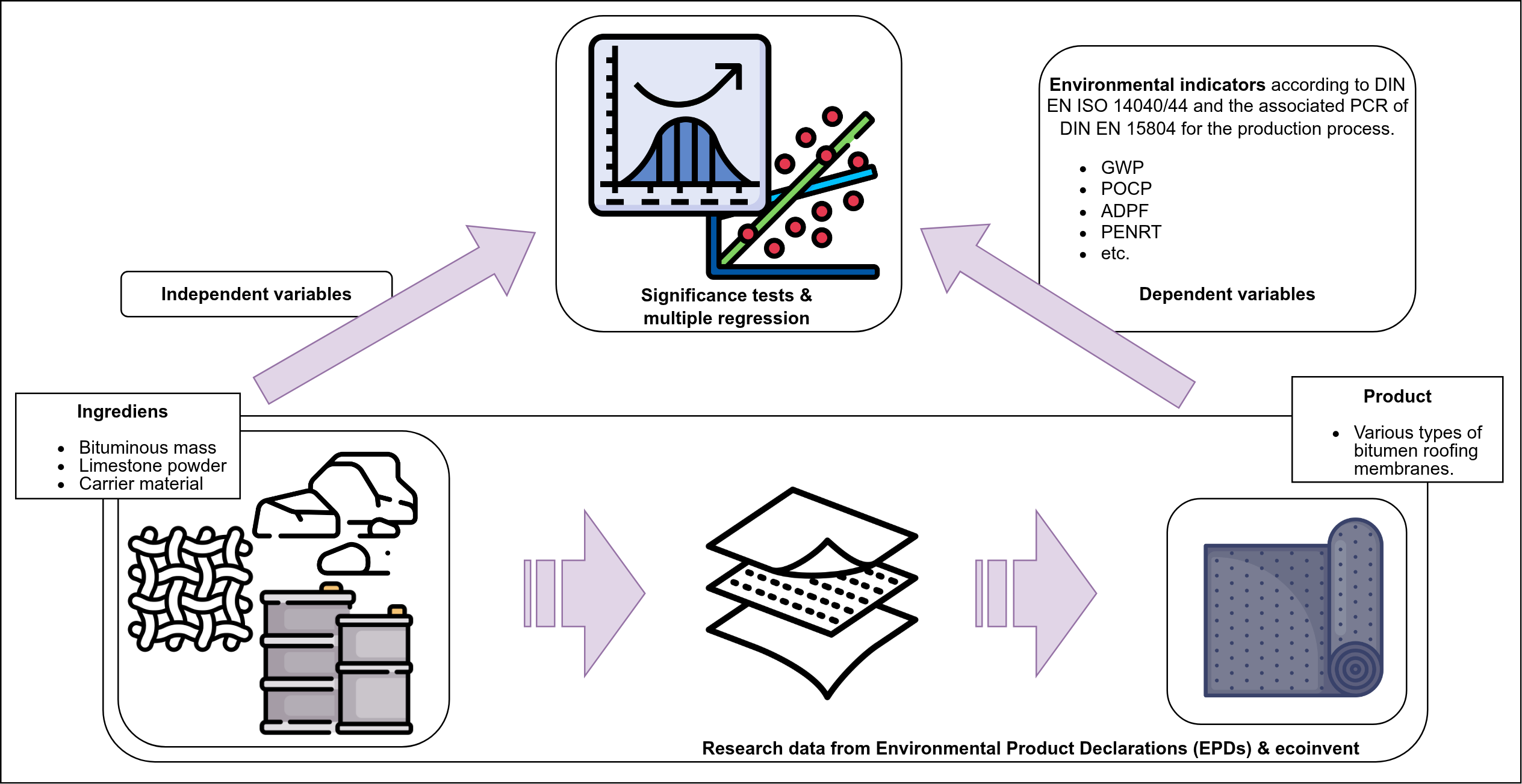
Bituminous roofing membranes are widely used construction materials for waterproofing applications and, due to their origin from crude oil, offer substantial sustainability potential in recycling contexts. Based on environmental indicators defined in current standards - the established standard for environmental product declarations - this study compiles a comprehensive overview from existing publications and investigates internal correlations as well as the influence of reinforcement layers. Classical statistical tools such as means, confidence intervals, and t-tests are primarily employed. In addition to linear approaches, a multiple regression model is introduced, enabling the prediction of environmental impact categories based on the input masses of bitumen and limestone filler. Except for four categories, statistically significant predictions are consistently demonstrated, with notably higher predictive performance for ADPE, EP-marine, GWP-fossil, and POCP compared to individual models. This ability to forecast environmental impacts in membrane production provides a robust basis for the planning and development of more environmentally friendly processes - an essential step toward a more sustainable, waterproof future.
Keywords:
bitumen sealing
; bitumen recycling
; circular construction
; correlation analysis
; predictability
; impact indicator
; construction products
; LCA
; EPD
1. Introduction
Bitumen is among the oldest known construction materials, with evidence of its extraction in Mesopotamia dating back several millennia. Historical records indicate that additives were used even then to modify its melting point. In addition to its role in construction, bitumen also found applications in early medicine [1]. Today, bitumen is predominantly employed in road surfacing and waterproofing applications. In Germany alone, the demand for bituminous sealing materials reached 63 million square metres in 2023 [2]. Given that approximately 60 % to 70 % of flat roofs in the country are covered with bituminous membranes, this figure is expected to rise [3]. While there is a growing demand for housing and usable space, the service life of waterproofing systems remains limited due to environmental exposure, UV radiation, and natural ageing. Consequently, replacement is typically required every 30 to 50 years [4].
Bitumen, a crude oil derivative, is not only a high-energy raw material, but also offers significant material reuse potential. This potential is already being explored through the recycling of road construction bitumen [5,6,7]. Life Cycle Assessments (LCAs) serve as a key methodology in evaluating such potential, analysing environmental impacts across the entire product lifecycle. These assessments are instrumental in comparing different materials and identifying opportunities for environmental optimisation, as demonstrated in studies on polymer-based roofing membranes [9]. In addition to methodological considerations, [12] emphasised the capacity of LCAs to investigate trends - illustrated here through the example of roofing in the construction sector - and to identify opportunities for further development. Reusing bituminous mass from roofing membranes presents a logical and environmentally beneficial approach, as the majority of emissions are attributed to the initial bitumen production, followed by transport and energy consumption [8,11].
Fundamentally, bituminous roofing membranes are composed of four principal components: the bitumen binder (typically comprising oxidised bitumen with additives); mineral fillers such as limestone powder; protective surface layers (e.g. sand or slate) that guard against mechanical and thermal stress; and a reinforcement layer made from materials such as synthetic fibres, glass fibre, aluminium, or felt, which imparts specific technical properties to the membrane [10].
To provide a contextual foundation before delving into detailed analyses, estimations were made based on the available sample in order to describe observed trends and support a well-grounded understanding of the environmental influences associated with bituminous sealing materials. Given the partial overlap among several environmental impact categories, it is assumed that certain interdependencies may exist particularly among AP, EP (Eutrophication Potential), GWP, ODP, POCP, PENRT, and PERT [17]. To explore a more comprehensive understanding of the environmental impacts caused by the production of bituminous membranes, and to investigate whether meaningful relationships exist between the input-related indicators ADPE, ADPF, PENRT, and PERT and the output-related impact categories, a statistical examination of potential correlations was undertaken. This line of inquiry leads to a central question: Is there a measurable interaction between these indicators during the production process, and if so, how strong is ist?
In addition to the collection of data across 15 environmental indicators, supplementary information was obtained regarding the composition of the membranes specifically the types of carrier materials used (e.g. glass fibre, polyester, aluminium) as well as the relative proportions of bitumen mass and mineral fillers. Carrier layers play a key role in defining the mechanical properties of the membranes, tailored to meet different application requirements. These materials, however, also entail varying production methods, which may influence the overall environmental impact due to differences in energy demand and emissions. Although comprehensive production-specific data for these materials is limited, it appears promising to investigate whether distinct combinations of carrier materials correspond to significant variations in environmental indicators. This analysis may help determine whether the selection of a particular carrier material contributes measurably to the ecological performance of the membrane system.
Building upon these considerations, the question arises as to whether the environmental impacts of bituminous sealing membranes can be quantitatively predicted based on the material masses used -particularly bitumen and limestone filler. To this end, the study examines whether robust relationships between the quantities of these primary constituents and the resulting environmental indicators can be identified through the application of appropriate regression models. The aim is to develop a simplified, data-driven forecasting tool that enables early-stage estimation of ecological impacts during the planning process.
2. Methodology
2.1. Impact Categories
The current study takes into account fifteen impact categories to quantify environmental burdens arising from the emission of chemical substances into the environment. These categories are based on the requirements of [25] (Annex C), and are further explained by [23] (p. 200 ff.) and [24] (p. 109 ff.). Following standardised procedure, the impact assessment is formally conducted according to stage A2 of the aforementioned DIN EN 15804.
Abiotic depletion potentials are differentiated into two categories: elements (ADPE) and fossil resources (ADPF). These summarise the consumption of finite resources measured in kg Sb-eq. for ADPE and MJ (megajoules) for ADPF. ADPE is significantly influenced by rare elements such as gold, tellurium, platinum, and silver, while ADPF mainly comprises fossil fuels such as coal, natural gas, and crude oil.
Nitrogen-based emissions are captured primarily under the acidification potential (AP) and the eutrophication potentials for terrestrial (EP-terrestrial) and marine (EP-marine) ecosystems, including nitrogen oxides, ammonia, and nitrate compounds. The acidification potential (AP) also includes sulphur dioxide and related compounds, while the freshwater eutrophication potential (EP-freshwater) predominantly reflects phosphorus-based emissions. The commonly applied units are mol H-eq. for AP, mol N-eq. for EP-terrestrial, kg N-eq. for EP-marine, and kg P-eq. for EP-freshwater. As noted by [23] (p. 224), “Point sources in the form of wastewater treatment plants for households (e.g. from polyphosphates in detergents) and industry as well as fish farming are important sources of phosphorus and nitrates."
The most prominent impact category in the construction sector is the global warming potential (GWP). Common greenhouse gases contributing to GWP include carbon dioxide, methane, nitrogen oxides, and halogenated hydrocarbons, all standardised to the reference unit kg CO-eq. In order to better trace the sources of emissions, the GWP is subdivided into three categories: biogenic, fossil, and land use and land-use change (LULUC). These reflect emissions from biomass use and decay, fossil carbon oxidation, and carbon stock changes due to land use, respectively. GWP-total represents the sum of these subcategories and is calculated over a standardised time horizon of 100 years. As [23] (p. 207) state, “GHG emissions are attributable to almost any human activity. The most important contributing activities are: burning of fossil fuels and deforestation.”
The ozone depletion potential (ODP) accounts for substances that contribute to stratospheric ozone layer degradation, such as halogenated hydrocarbons, methane, nitrogen dioxide, bromine, and chlorine compounds. These are commonly associated with fire suppressants, insulating foams, and agricultural chemicals, and are measured in kg CFC-11-eq.
Photochemical ozone creation potential (POCP), often referred to as "summer smog", describes the formation of ground-level ozone due to photochemical reactions involving volatile organic compounds (VOCs) and carbon monoxide in the presence of nitrogen oxides and sunlight. Relevant substances include alkenes, aldehydes, ketones, alkanes, and halocarbons, with impacts expressed in kg NMVOC-eq. (non-methane volatile organic compounds).
The cumulative energy demand of a product or process is represented by the categories PERT (primary energy from renewable sources, total) and PENRT (primary energy from non-renewable sources, total). Both are measured in MJ, with PERT comprising inputs from water, wind, solar, and biomass energy, while PENRT includes fossil fuels and uranium. It is important to note that while ADPF and PENRT are largely overlapping in scope, the latter additionally includes energy contributions from peat and uranium, while biomass is accounted for only in PERT.
Finally, the water depletion potential (WDP) quantifies the relative potential of freshwater withdrawals to cause water stress, considering both availability and local demand. WDP is measured in cubic metres (m³) of water, whereby a high value indicates that water consumption is significant or takes place in water-scarce areas.
For analytical purposes, the indicators used here can be grouped into two general categories. On the one hand, ADPE, ADPF, PENRT, and PERT are classified as input indicators, which quantify raw material consumption and energy demand, representing indirect environmental pressure. On the other hand, the remaining indicators are output-based impact categories that reflect direct environmental consequences of emissions or resource use.
2.2. Database
All data used to investigate the manufacturing processes of bituminous roofing membranes were sourced primarily from publicly available Environmental Product Declarations (EPDs), with the exception of five membranes from the Ecoinvent database [37]. Initial information was drawn from the Ecoinvent and Ökobaudat databases [38]. These were subsequently supplemented with increasingly specific datasets from industry benchmarks provided by European Waterproofing Association (EWA), Hasse GmbH & Co. KG, and the roofing membrane manufacturers Phønix Tag Materialer (PTM) and Danosa. In total, 26 datasets were compiled (see Table A1 and Table A2). The data collected are broadly representative of the European market and were published between 2007 and 2021. A EPD assess products or product groups using environmental indicators in accordance with [26] and [25]. These results were selected to ensure the highest possible degree of comparability, despite the considerable methodological flexibility permitted in the compilation of product declarations [12].
The environmental impact categories (as outlined in Section 2.1) used for assessing the manufacturing phase (modules A1-A3, cradle-to-gate) are calculated as synthetic balances of material and energy inputs and corresponding emissions. The chemical outputs are classified into categories, weighted according to their relative environmental impact, and summarised across 13 emission-based indicators and two cumulative energy indicators. Each is reported in a standardised unit per kilogram of material. To ensure comparability between products of varying thickness, all indicators were normalised by dividing the impact values by the area-related mass (expressed in kg per m). This approach yields, for example, a unit of kg CO-equivalent per kg of material in the case of the GWP, effectively isolating the influence of sheet thickness on the results.
All applied methods as follows and the corresponding datasets used for the analysis are summarised in Table 1. This table provides an overview of the methodologies employed in the study, alongside the specific data sources utilised in processing the bitumen roofing membrane data. Since Hasse’s results used many different carrier materials, these were excluded from the significance tests, as were two of the Ökobaudat roofing membranes. The second of these were excluded because glass was significantly underrepresented in the sample. The results from the Ecoinvent database represent scientifically reliable values, but they have not been verified in accordance with standard norms and were therefore only used to provide an overview. Since the Ökobaudat platform does not publish any information on the composition of roofing membranes, this information was also not excluded in the regression analyses.
2.3. Overview
To provide an initial overview of the dataset and to estimate characteristics of the underlying population, descriptive statistical measures including mean values, standard deviations, and 95 % confidence intervals were calculated based on the full sample of 26 products (N=26) ([15], p.353 ff.). These statistical methods are well established in empirical research and represent the minimum standard required to adequately describe and interpret survey data.
2.4. Pearson Correlation Coefficients
Correlation analysis provides an efficient method for identifying both the strength and direction of relationships between two variables. When dealing with multiple variables, it is common practice to present all pairwise correlations within a matrix format to allow for a clear and descriptive overview.
In this study, Pearson correlation coefficients (r) were calculated for all combinations of the selected environmental indicators. These coefficients are presented in a triangular matrix format for improved clarity and interpretability. In addition, significance testing was conducted to assess the likelihood that the observed correlations occurred by chance. The thresholds proposed by [14]1 ( p.77 ff.) were applied to interpret the strength of correlations, and statistical significance was evaluated using two-tailed t-tests.
Due to the generic nature and relatively low specificity of the Ecoinvent dataset, its results are considered highly variable [26,43]. Consequently, only data from Hasse, Ökobaudat, Phønix Tag Materialer (PTM), EWA, and Danosa (see Table 1) were used for the correlation analysis. This adjustment reduced the effective sample size to 21 roofing membrane products (N=21).
2.5. Statistical Significance Testing
The remaining carrier materials were grouped into four categories: aluminium (n=1), glass fibre (n=3), polyester (n=10), and a glass-polyester composite (n=7). As aluminium and glass fibre category comprises only one and three entries, they are not considered representative and lacks sufficient statistical power to yield meaningful results (Table A1). With the dataset reduced to two material categories - polyester and glass-polyester composites (N=17) - a two-tailed significance test was conducted to compare group means and examine the null hypothesis (H) that no true difference exists between them [18]. Due to the unequal group sizes and potential heterogeneity of variances, Welch’s t-test was applied instead of the standard Student’s t-test ([15], p.452-453).
2.6. Regression Analysis
The variables representing the mass ratios of bitumen and limestone were included as independent variables in the following analyses. Precise formulations regarding plasticisers, tyre-derived additives, or oils were not available and could therefore not be considered. Similar to correlation analysis, linear regression was used to model the relationship between two variables and to quantify the proportion of variance explained by the fitted model. This is represented by the coefficient of determination (R), which indicates the percentage of the total variance in the dependent variable that is explained by the model ([15], p. 245 ff., p. 711 ff.). Before performing regression modelling, the degree of multicollinearity between the two independent variables - bitumen mass ratio and limestone (mineral) mass ratio - was examined to ensure the validity of subsequent interpretations ([15], p. 742).
In addition to assessing general trends, the regression models aim to determine which of the two materials has a greater predictive influence on specific environmental indicators or whether one exhibits an inverse relationship. To this end, three separate regression models were developed for each environmental indicator:
- Bitumen mass ratio vs. limestone mass ratio
- Bitumen mass ratio vs. indicator
- Limestone mass ratio vs. indicator
Finally, a multiple linear regression model was constructed for each indicator using both bitumen and limestone mass ratios as predictors. This allows for the evaluation of whether the combined contribution of both materials provides a better explanation of variance than each single predictor alone. The statistical significance of each regression model was assessed using the F-statistic, which compares the variance explained by the model with the unexplained variance (i.e. the residual variance) relative to the overall mean of the data ([15], p. 500 ff.). Due to the limited material-specific data available in the Ökobaudat dataset and the high variability observed in the Ecoinvent values, the sample size available for variance comparisons is restricted. Consequently, the three variable groups - bitumen mass ratio, mineral mass ratio, and environmental indicator (k=3) - were analysed based on the 17 roofing membrane products drawn from the datasets provided by Hasse, Phønix Tag Materialer (PTM), EWA, and Danosa (N=17).
2.7. Calculation Software
Python (v3.11.8) was used for data handling, exploratory analysis, and correlation tasks, while significance testing and regression analyses were conducted using RStudio (v2024.12.1).
3. Results
3.1. Overview
Table 2 presents the results from the initial calculations across the entire survey. The means and their corresponding confidence intervals of the most categories show low values close to zero, with the exceptions of ADPF, GWP-biogenic, GWP-fossil, GWP-total, PENRT, PERT, and WDP. Of particular interest is the observation that the means and standard deviations for GWP-fossil and GWP-total are identical. This reflects the fact that GWP in the assessed datasets is measured in CO-equivalents and stems almost exclusively from fossil inputs, with negligible biogenic contributions.
A closer look at ADPF and PENRT reveals that both indicators account for the quantities of gas, oil, and other fossil-based materials. However, PENRT consistently reports values approximately 1.7 MJ higher than ADPF, with comparable precision (see Table 2, CI 95 %). At this stage, it remains unclear whether these fossil inputs are primarily used as membrane materials or as energy sources during production.
In contrast, the contribution of renewable energy - summarised in the PERT category - remains relatively low, with a mean of 1.6 MJ and a narrow variance (ranging from 1.2 MJ to 1.9 MJ). These values suggest that renewable energy sources such as wind and hydro play a limited role in current production processes. Nevertheless, their contribution is shaped by multiple systemic factors, including infrastructure availability, the electrification of production stages, and regional energy policies. Although PERT cannot directly reflect fossil fuel substitution, it offers valuable insight into the renewable share in overall energy demand.
Finally, the results for WDP show that the production of bituminous membranes consumes between 171 and 398 litres of water. This wide range highlights the considerable uncertainty associated with water-related impacts, which appear to be influenced by factors such as product type, carrier material, bitumen content, and geographic production conditions.
3.2. Pearson Correlation Coefficients
The triangular correlation table (dof = 19) is included in Appendix A3 due to its large size, consisting of 15 by 15 dimensions. To present the numerous covariations between the indicators clearly, it is important to note that most show high and statistically significant correlation coefficients. Given the previously established interdependence of the impact categories - AP, EP, GWP, ODP, POCP, PENRT, and PERT - it is unsurprising that numerous correlations with high statistical power are observed. For instance, ODP interacts with nearly all other categories, except for EP-freshwater (r=.36, p=.106), GWP-fossil (r=.15, p=.523), and GWP-total (r=.14, p=.559). Conversely, EP-freshwater exhibits few significant correlations with other indicators, with the exceptions of ADPE (r=.77, p<.000) and POCP (r=.60, p=.004).
The ODP, associated with substances such as hydrocarbons, chlorines, and halogens, appears strongly linked to the production process, in contrast to phosphorus emissions, which primarily vary in relation to effects on stratospheric ozone depletion. Several combinations of indicators, within the 5 % error probability, are statistically significant, with some correlations exceeding 0.90. The perfect correlation between GWP-total and GWP-fossil (r=1.00, p<.000) clearly reflects the previously mentioned dependence on fossil resources in the GWP indicator. The eutrophication categories EP-terrestrial and EP-marine (r=.98, p<.000) show a near-identical correlation, which can be attributed to their overlap in ammonium and nitrogen compounds. The depletion of fossil resources (ADPF) correlates strongly with the primary energy indicators of PENRT (r=.97, p<.000), as both categories consider almost exclusively the same fossil materials.
GWP-biogenic exhibits a stronger predictive performance in relation to PENRT (r=.84, p<.000) and ADPF (r=.84, p<.000) compared to GWP-fossil (r=.52, p=.016; r=.59, p=.005). This is due to the fact that GWP-biogenic includes only emissions from biogenic or non-fossil sources, such as methane and carbon dioxide, making it more predictable than GWP-fossil, which also accounts for additional substances, including sulfur, nitrogen, and hydrocarbons.
The three correlations between AP and EP-marine, EP-terrestrial, and GWP-luluc are exactly 0.90 (p<.000), revealing that land use, as well as EP-marine and EP-terrestrial ecosystems, are closely linked to the acidification of the environment. Furthermore, the eutrophication of seawater and terrestrial ecosystems, particularly influenced by nitrogen compounds, shows strong correlations with the GWP of land use (r=.80, p<.000; r=.87, p<.000), which is primarily represented by CO and hydrocarbons, associated with the conversion of natural ecosystems into managed ecosystems ([20], p. 96).
The use of elementary resources in ADPE, or their provision, serves as a reliable predictor for ozone creation potential (POCP, r=.89, p<.000), which is also strongly influenced by hydrocarbons ([19], p. 51, ff.). Furthermore it covariates strong with the above mentioned group of acidification, eutrophications, land use and ozone depletion potential.
Reciprocal correlations are observed for primary renewable energies in PERT with ADPE (r=-.56, p=.008), AP (r=-.81, p<.000), EP-marine (r=-.61, p=.004), EP-terrestrial (r=-.60, p=.004), GWP-luluc (r=-.65, p=.002), ODP (r=-.74, p<.000), POCP (r=-.60, p=.004), and WDP (r=-.73, p<.000). An increasing share of renewable, eco-friendly energy sources is associated with a reduction in impact categories, which can be linked to a decrease in the use of elements and fossil fuels. The lack of significance in the regression analysis of ADPF and GWP-fossil with PERT indicates that the variation in both energy resources cannot be correlated with each other.
Water consumption in WDP is predicted by decreasing values in ADPF (r=-.66, p=.001), GWP-biogenic (r=-.70, p<.000), PENRT (r=-.64, p=.002), and PERT (r=-.73, p<.000). Conversely, water demand is also correlated with impacts such as AP (r=.66, p=.001) and ODP (r=.86, p<.000), which are linked to chemicals that affect the environment through acidification or depletion of the ozone layer.
Finally, it can be concluded that if the ADPE and ADPF values are considered as “inputs” into the process and all other impact categories as “outcomes”, each indicator can be predicted with a minimum correlation coefficient of r=.56 (absolute) and p=.008.
3.3. Welch Test
Table 3 presents the results of the Welch test for all environmental indicators, displaying the test statistics and their associated power. To ensure transparency, the table includes not only the t-value, p-value, and mean and standard deviation estimates for both groups, but also the degrees of freedom, confidence intervals, and Cohen’s d, offering a deeper insight into the statistical outcomes.
With regard to the significance level of 5.0 %, three tests provide robust results: ADPF (t=2.5, p=.028), PENRT (t=2.3, p=.039), and WDP (t=-2.3, p=.048). The effect size (Cohen’s d) for these results ranges between 0.60 and 0.63, which can be interpreted as a medium effect. Therefore, it is also meaningful to consider the impact category ODP (t=-2.2, p=.059) with a Cohen’s d of 0.62 in the interpretation of the results.
The significance of ADPF and PENRT clearly indicates that the influence of the layer material in the production process varies according to the effort expended on fossil materials. Both indicators demonstrate similar levels and variations, and the observed effect size is comparable.
Furthermore, the WDP (t=-2.3, p=.048) also shows significance when distinguishing between the carrier materials with respect to the 5 % probability of error. The mean difference nearly includes zero (see CI 95 %), which can be interpreted as both groups being equal. This may be explained by the high variance of the WDP within the glass group (M_g=.15, SD_g=.20), what theoretically allows a overlap to negative values.
A similar phenomenon is observed in the case of ODP (t=-2.2, p=.059). Although the results of the balances are very small (M_g=.000 000 018, M_pg=.000 000 072), the effect size remains high, which can be seemingly attributed to one of the two carrier materials used.
Even if the primary renewable energies are barely significant here (PERT; t=2.1, p=.06), they exhibit a relatively low spread and also tend to be distinguishable. This points to a potentially meaningful effect, which might become significant with a larger sample size or more homogeneous data.
3.4. Regression Analysis
The major compositions of the coating mass are 33 % to 75 % raw bitumen and 18 % to 42 % mineral mass (Table A1). The bitumen itself can be linked almost directly to the environmental indicators and the high proportion of both materials in the total product mass can be a good basis for estimating the magnitude of emissions.
Table 4 presents the interactions between the bitumen and limestone mass ratios. Although the intercept shows a significant value of 0.37, the slope (coefficient) explains very little of the variations in the model (r = .0034, F=.051, p=.824). Due to the low dependency between the amount of bitumen and the limestone mass, it can be concluded that there are no notable interactions between these two ingredients. This indicates that the quantities of bitumen and limestone in the mixture do not affect each other, thus facilitating a better understanding of these components as predictors in the subsequent multiple regression analyses.
The covariance between the bitumen or mineral proportions and the indicators leads to two additional regression models, presented in Table 5 and Table 6. The first of these contains 12 regressions that describe the indicator values based on the variation in the bitumen content, according to the 5 % significance level. Half of these regressions show a moderate explanation of variance (r>.13), while the other half indicate a high explanation of variance (r>.26), in line with [14], p. 79 ff.) conventions.
More than 50 % of the overall variation in the indicators can be explained by the following impact categories: ADPE (r=.75, F=46.1, p<.000), AP (r=.53, F=17.1, p=.001), ODP (r=.61, F=23.2, p<.000), and POCP (r=.64, F=26.7, p<.000). The proportion of bitumen in a roofing membrane provides a reliable indicator of the emissions of compounds such as ammonia, sulfur, hydrocarbons, and halogens during the manufacturing process, all of which decrease as the bitumen mass input increases (see Table 5). Similarly, the ADPE impact category is affected, showing a reduced intake of elementary substances such as gold, silver, and palladium.
The reduction in nitrogen, nitrate, and ammonia emissions with an increasing bitumen mass is reflected in the EP-marine (r=.35, F=8.1, p=.012) and, like the energy requirement (PERT) (r=.38, F=9.2, p=.008), both describe more than a third of the covariance between the values. PERT is the only significant indicator that shows a positive correlation with the coating mass, and it behaves similarly to the demand for fossil fuels (PENRT) (r=.23, F=4.5, p=.052); both increase as the bitumen proportion rises.
An examination of the coefficients in Table 5 further reveals that higher bitumen content is associated with increased values in the ADPF and PENRT categories.
In an attempt to predict the environmental impacts based on the proportion of minerals, six reliable regression models, almost all with high r coefficients, were identified, with each model displaying a negative slope, except for PERT. The ADPF (r=.28, F=5.9, p=.028) and PENRT (r=.27, F=5.4, p=.034) indicators both tend to decrease as more minerals are used as fillers in the recipe, reflecting the strong influence of fossil resources.
A similar trend is observed for the EP-marine (r=.24, F=4.7, p=.048), GWP-fossil2 (r=.45, F=12.1, p=.003), and POCP (r=.26, F=5.4, p=.035) emissions. The quantity of ammonium and nitrogen compounds in EP-marine, or the proportion of carbon dioxide and hydrocarbons in GWP-fossil and POCP, decreases with higher limestone content. Nearly half of the variation in GWP values can be explained by this relationship.
In contrast to the aforementioned trends, the two primary energy indicators, PENRT and PERT (r=.18, F=3.2, p=.093), exhibit exactly the opposite behaviour, as evidenced by their coefficients. A higher proportion of fillers appears to correlate with an increase in renewable energy inputs and a decrease in fossil energy inputs.
Both Table 5 and Table 6 - i.e., both sets of analyses - demonstrate that the regression models are robust for several different indicators. Taken together, 14 of the 15 indicators (excluding GWP-biogenic) can be described with a minimum r of 0.27 using the regression models, based either on bitumen or mineral content.
The combination of both regression approaches results in a multiple regression model for each indicator. To present the results adequately, a comprehensive table is provided in the appendix, which consolidates the estimated intercepts and coefficients, the p-values, the adjusted R, and the F-statistics (Table A4).
Four of the generated regression models do not show significant results for predicting the indicators ADPF (R=.23, F=3.4, p=.062), GWP-biogenic (R=.02, F=1.2, p=.332), GWP-luluc (R=.14, F=2.3, p=.139), and WDP (R=.15, F=2.4, p=.131). For these indicators (with the exception of GWP-biogenic), the multiple regression approach yields lower R values (below 0.263) and less significance (p-values above 0.05), with F-values lower than the critical value (F=3.739) compared to the models based on a single criterion.
The impact categories with the most significant results and the highest explained variances are POCP (R=.95, F=148.6, p<.000), ADPE (R=.92, F=90.2, p<.000), GWP-fossil (R=.71, F=20.9, p<.000) and ODP (R=.64, F=15.0, p<.000). The near-perfect covariation between bituminous and mineral substitutes with POCP demonstrates how precisely this indicator can be predicted by both raw input materials, in relation to their effectiveness in emitting hydrocarbons (non-methane volatile organic compounds) from power plants, traffic, coatings, and binders. This may also explain the strong regression with elements in ADPE, which are required for sustaining processes and machinery. Hydrocarbons, fluorine compounds, and various refrigerants resulting from industrial processes also influence the GWP-fossil and ODP indicators.
The concise multiple regression models for the AP (R=.59, F=12.4, p=.001), EP-terrestrial (R=.39, F=6.1, p=.013), and EP-marine (R=.62, F=11.6, p=.001) indicators show considerable overlap in their measurement scope. Due to the common detection of ammonia and other nitrogen compounds, these indicators are strongly correlated with each other, whereas AP is more influenced by energy generation using fossil materials, while the eutrophication potentials are primarily influenced by land-use changes, agriculture, and wastewater. These are typical factors that arise in production processes.
The EP-freshwater (R=.28, F=4.0, p=.041) also exhibits a significant degree of explained variance, which can be attributed to phosphorus and phosphate inputs. EP-freshwater is strongly correlated with ADPE and POCP (Table A3), despite the relatively minor influence of phosphorus in these two impact categories ([21], [21]; [22], [22]).
Finally, the total primary energy indicators - renewable PERT (R=.53, F=10.0, p=.002) and non-renewable PENRT (R=.39, F=6.1, p=.012) - account for approximately 53 % and 39 % of the model performance, respectively. The adjusted R for PERT is nearly as high as the sum of the regression models with just a single criterion.
The coefficients of determination (R) for the ADPE, EP-marine, GWP-fossil, and POCP indicators from the multiple regression models are higher3, thereby explaining a greater proportion of the variance in the results than would be explained by summing the r values from the single-criterion models (Table 5 and Table 6).
4. Discussion
4.1. Correlation Matrix
A strong correlation between environmental indicators implies that the analysed production process emits substances which influence both categories to a similar extent when considered in weighted aggregate. This shared set of substances allows for the derivation of a relationship between the indicator values, enabling the characterisation of the process from a life cycle accounting perspective.
- Expenditures of fossil raw materials can serve as significant predictors, particularly for the biogenic GWP and non-renewable primary energy demand, both of which show a negative correlation with water consumption.
- In contrast, acidification potential, eutrophication, ozone depletion potential, and photochemical ozone creation potential can be well estimated by the use of elemental substances, which are negatively associated with the use of renewable primary energy sources.
Fossil and mineral raw materials also form, according to [28], alongside land use, a robust basis from which the majority of other emissions can be estimated. Similarly, [29] identify key indicators that serve as levers for understanding interdependencies within production processes and for uncovering potential for optimisation. The existence of correlations between indicators is further confirmed by these findings, and their interrelations are sufficiently strong to be represented in a model that captures, to a large extent, the interdependencies present in the production of bituminous roofing membranes.
The results reflect a specific construct that establishes connections between numerous, highly diverse environmental categories. These interrelations must be interpreted within the context of roofing membrane production and do not constitute a generic forecasting tool. Although identical chemical compounds may contribute to different environmental phenomena, the magnitude of a weighted environmental equivalent cannot be directly derived from this alone.
4.2. Predicting Carrier Material
The comparison of different reinforcement materials within the production process provides insights into the environmental impacts associated with the various application areas of roofing membranes. Given the wide range of potential uses for roofing membranes, it is necessary to tailor sustainability-related development efforts to specific functional properties.
In particular, the use of fossil resources varies noticeably between the reinforcement types investigated - namely, polyester and a polyester–glass composite. This may be attributed to the comparatively higher fibre content of the composite product, which could result in a reduced bitumen share in the membrane. The WDP, as defined by [25], is subject to numerous assumptions and uncertainties, as previously discussed by [31], contributing to the considerable variability of these individual results. On average, these values exhibit an inverse trend to fossil resource use, potentially due to the doubled fibre production and the higher water scarcity associated with polyester production, as reported by [32].
The very low presence of ozone-depleting substances - such as refrigerants, blowing agents, or pesticides - can be traced back to regulatory actions, most notably the Montreal Protocol of 1987 [30], and are now primarily attributable to deconstruction activities or the improper disposal of electronic equipment.
A selective assessment of the impact categories suggests that increased use of reinforcement materials can lead to a reduction in environmental burdens related to fossil resource consumption. However, this benefit is offset by other effects - most notably water consumption - which highlights the importance of context-specific and regional decision-making in individual cases. The limited sample size restricts conclusions to the two reinforcement types examined. Furthermore, the inherent difficulty of accurately quantifying environmental impacts introduces considerable potential for distortion in the findings.
4.3. Regression Models
It can be concluded that no direct or indirect linear relationship is evident between the two base materials - bitumen and limestone filler mass - thus supporting the assumption of their mutual independence. Regression models using only one of these constituents already demonstrate strong predictive capabilities with regard to environmental indicators. However, when both constituents are combined within a single predictive approach, significantly higher - sometimes even superior - predictive accuracies can be achieved compared to the individual models.
Reduced to these two essential components of a bituminous roofing membrane, linear regression proves to be a versatile tool for simplifying the complex processes involved in production and for enabling quantitative estimations of emissions.
These findings, particularly concerning the regressive relationships between input materials, environmental indicators, and energy sources, align with the investigations of [34,35,36] (the latter of whom even applied machine learning techniques to develop a generic prediction tool for environmental impacts using training data from the ecoinvent database.
The analysis underscores the complexity of the issue at hand, which is shaped by numerous uncertainties. Variations in environmental databases, divergent calculation methodologies, the specificities of the examined production process, and, not least, the definition of system boundaries all complicate the development of a robust statistical model capable of delivering reliable predictions.
5. Conclusions
Climate change demands a more sustainable use of fossil resources, which remain essential components of conventional bituminous sealing membranes in the construction sector. In the planning and maintenance of buildings, long-term insights are increasingly important to enable the assessment and mitigation of environmental emissions.
From this research question, an average model of environmental impacts was developed. Through overviews and correlation analyses, the complex production process could be characterised from an environmental perspective. Subsequently, a predictive tool was established, capable of estimating impact categories based on the most significant input materials. A detailed differentiation based on reinforcement materials was not included at this stage. This perspective on the construction product "bituminous roofing membrane" can now serve as a foundation for targeted emission reductions - based on the formulation of current or newly developed membrane types. The analysis focused primarily on the European region over the past decades and incorporated data from various environmental databases. However, some roofing membrane types are underrepresented in current data sources which could be addressed in future studies by incorporating a broader range of data. This would not only allow for more precise evaluation of effect sizes but also help to reduce distortions arising from differing database structures and data collection methodologies.
A particularly relevant distinction for planners and building owners lies in the use of product-specific Environmental Product Declarations (EPDs) versus generic datasets. While generic data - as typically found in standard LCA databases - offer a rough orientation, they may either under- or overestimate environmental impacts due to averaging across multiple products, outdated processes, or lack of regional differentiation. EPDs, by contrast, provide verified, manufacturer-specific data that are aligned with real-world production and often include third-party verification. This distinction is critical in the context of sustainable building certification (e.g., DGNB, LEED) or material selection decisions, where reliance on generic datasets may lead to misinformed design strategies or missed opportunities for emission reduction.
The application of statistical tools in this context is well established and demonstrates considerable potential, particularly in the field of machine learning. Nevertheless, it must be emphasised that such results always represent probabilistic insights rather than deterministic constructs and an uncertainty or error analysis is also still to be performed.
Knowledge generation alone is insufficient if it does not lead to meaningful action. Climate change creates a pressing need for response while simultaneously offering an opportunity to identify potential, define targets, and establish processes that contribute to a stable and environmentally responsible future. Accordingly, this study should be understood as a starting point-offering a perspective upon which further innovation can be built. Investigative research is of critical importance, but it is equally vital that we do not fail to act upon its findings.
Author Contributions
Supervision, funding acquisition, resources, validation, writing - review, C. Thiel; investigation, conceptualization, formal analysis, methodology, data curation, writing - draft & editing, M. Schmid;
Funding
Publishing fee supported by the Open Access Publishing Fund of Ostbayerische Technische Hochschule Regensburg during the project work funded by Zukunft Bau Forschungsförderung.
Acknowledgments
I would like to express my sincere gratitude to my colleagues and fellow researchers for their valuable discussions and encouragement throughout the course of this work. I am also thankful to the many curious students whose questions and perspectives have, even indirectly, contributed to the development of this study.
Conflicts of Interest
The authors declare no conflicts of interest.
Abbreviations
The following abbreviations are used in this manuscript:
| ADPE | Abiotic Depletion Potential of Elements |
| ADPF | Abiotic Depletion Potential of Fossils |
| AP | Acidification Potential |
| DGNB | Deutsche Gesellschaft für Nachhaltiges Bauen |
| EP | Eutrophication Potential |
| EWA | European Waterproofing Association |
| EPD | Environmental Product Declaration |
| GHG | Greenhouse Gas |
| GWP | Global Warming Potential |
| LEED | Leadership in Energy and Environmental Design |
| LULUC | Land-Use and Land-Use Change |
| MDPI | Multidisciplinary Digital Publishing Institute |
| NMVOC | Non-Methane Volatile Organic Compounds |
| LCA | Life Cycle Assessment |
| ODP | Ozone Depletion Potential |
| PENRT | Primary Energy Non-Renewable, Total |
| PERT | Primary Energy Renewable, Total |
| POCP | Photochemical Ozone Creation Potential |
| VOC | Volatile Organic Compounds |
| WDP | Water Depletion Potential |
Appendix A. Materials & Results
Appendix A.1. Used Datasets
Declarations for datatable A.1:
- [1]
- Geogr. allocation Ecoinvent: https://geography.ecoinvent.org/#list-of-locations-in-ecoinvent.
- [2]
- Average value from general product research.
- [3]
- Bitumen sheets with emission deviations < 10 % are summarized by the manufacturer.
- [4]
- Assumption based on the density.
- [5]
- Up to 18.72 % recycled bitumen (recycled oil compounds, tank cleaning) 100 % ash (biomass). 50 % polyester (recycled LDPE).
- [6]
- Weighted mass-based average of total production.
- [7]
- Results from A1 to A3 converted to 35 years lifespan (without renewal).

Table A1.
EPD findings of bitumen roofing sheets of different sources.
| Source | Product | Carrier | Density [] | Thickness [mm] | Bitumen ratio | Mineral ratio | Year ref. | Geography | Database |
| Hasse | Yearly production | Glasfiber, Polyester fleece, Aluminium | 5.40 [6] | 4.17 [6] | 0.33 | 0.27 | 2021 | DE | Ecoinvent 3.9 |
| Ökobaudat | G200 S4 | Glas fiber | 5.0 | 4.0 | - | - | 2018 | DE | GaBi |
| PYE PV200 S4 | Polyester fleece | 5.21 | 4.0 | - | - | 2018 | DE | GaBi | |
| PYE PV200 S4 ns | Polyester fleece | 6.20 | 4.0 | - | - | 2023 | DE | GaBi | |
| V60 | Glas fleece | 5.0 | 4.0 [4] | - | - | 2023 | DE | GaBi | |
| Ecoinvent | Alu80 | Aluminium | 1.9 [2] | 1.5 [2] | 0.66 | 0.24 | 2007 | RER [1] | Ecoinvent 3.10 |
| EP4 | Polyester fleece | 4.7 [2] | 4.00 | 0.57 | 0.30 | 2007 | RER [1] | Ecoinvent 3.10 | |
| PYE PV200 S5 | Glas fiber | 6.02 [2] | 5.00 | 0.63 | 0.18 | 2007 | RER [1] | Ecoinvent 3.10 | |
| V60 S4 | Glas fleece | 5.76 [2] | 4.00 | 0.71 | 0.26 | 2007 | RER [1] | Ecoinvent 3.10 | |
| VA4 | Glas fleece / Aluminium | 5.33 [2] | 4.00 | 0.72 | 0.14 | 2007 | RER [1] | Ecoinvent 3.10 | |
| Phønix Tag Materialer | AeroTæt PF2000 | Polyester fleece | 2.24 | 2.10 | 0.54 | 0.42 | 2021 | DK | GaBi 10.6.1.35 |
| Aero Tæt PF3200 | Polyester fleece | 3.39 | 2.90 | 0.54 | 0.42 | 2021 | DK | GaBi 9.2.1.68, Ecoinvent 3.6, Eurobitume LCI 2019 | |
| BituFlex PF5000 SBS | Polyester fleece | 5.00 | 4.30 | 0.545 | 0.365 | 2021 | DK | ||
| BituFlex Kombi PF/GF5000 SBS | Polyester fleece / Glas fleece | 5.30 | 4.40 | 0.545 | 0.365 | 2021 | DK | ||
| DuraFlex PF3500 SBS | Polyester fleece | 3.30 | 2.90 | 0.545 | 0.365 | 2021 | DK | ||
| DuraFlex Kombi PF/GF3500 SBS | Polyester fleece / Glas fleece | 3.30 | 2.90 | 0.545 | 0.365 | 2021 | DK | ||
| Topmembran PF4600 SBS | Polyester fleece | 5.00 | 4.70 | 0.635 | 0.235 | 2021 | DK | ||
| Flammespærre GF3000 | Glas felt | 2.54 | 2.00 | 0.54 | 0.42 | 2021 | DK | ||
| Bundmembran PF4500 SBS | Polyester fleece | 5.10 | 4.70 | 0.635 | 0.235 | 2021 | DK | ||
| European Waterproofing Association | Benchmark [7] | Polyester and glas fleece | 5.30 | 4.30 | 0.485 | 0.355 | 2019 | BE BY DK FI FR DE IT LT NL NO PT RU ES SE | SimaPro 9, Ecoinvent 3.6, Plastics Europe 2014 |
| Danosa [3][5] | System NTV2/EXT1 | Polyester fleece, Glas fiber | 8.64 | 5.0 | 0.475 | 0.34 | 2021 | Intern. | Ecoinvent 3.8, SimaPro 9.3 |
| System TPP1/NTG1 | Polyester fleece, Glas fiber | 7.96 | 5.8 | 0.475 | 0.34 | 2021 | Intern. | Ecoinvent 3.8, SimaPro 9.3 | |
| System TVA1/TVH1/TPC1/TPC2 | Polyester felt / Glas fiber | 9.04 | 6.15 | 0.475 | 0.34 | 2021 | Intern. | Ecoinvent 3.8, SimaPro 9.3 | |
| ESTERDAN PLUS 50/GP ELAST | Polyester fleece | 6.0 | 3.5 | 0.475 | 0.34 | 2021 | Intern. | Ecoinvent 3.8, SimaPro 9.3 | |
| POLYDAN PLUS FM 50/GP ELAST | Polyester felt / Glas fiber | 5.6 | 3.5 | 0.475 | 0.34 | 2021 | Intern. | Ecoinvent 3.8, SimaPro 9.3 | |
| System NTV6 | Polyester fleece | 7.84 | 5.0 | 0.475 | 0.34 | 2021 | Intern. | Ecoinvent 3.8, SimaPro 9.3 |
Table A4.
Models of multiple regression for each impact category (dof = 2, dof = 14).
| Estimate | p-value | R (adj.) | F | ||
| ADPE | Intercept | 1.622e-05*** | >0.000*** | 0.92 | 90.2 |
| Prop. bitumen | -2.100e-05*** | ||||
| Prop. minerals | -1.252e-05*** | ||||
| ADPF | Intercept | 30.50* | 0.062* | 0.23 | 3.4 |
| Prop. bitumen | 45.03** | ||||
| Prop. minerals | -67.91** | ||||
| AP | Intercept | 0.014746*** | 0.001*** | 0.59 | 12.4 |
| Prop. bitumen | -0.017761*** | ||||
| Prop. minerals | -0.009922* | ||||
| EP-freshwater | Intercept | 1.778e-04*** | 0.041** | 0.28 | 4.0 |
| Prop. bitumen | -1.954e-04** | ||||
| Prop. minerals | -1.669e-04 | ||||
| EP-terrestrial | Intercept | 0.019096*** | 0.013** | 0.39 | 6.1 |
| Prop. bitumen | -0.014530** | ||||
| Prop. minerals | -0.017036** | ||||
| EP-marine | Intercept | 0.0020376*** | 0.001*** | 0.62 | 11.6 |
| Prop. bitumen | -0.0017022*** | ||||
| Prop. minerals | -0.0018224*** | ||||
| GWP-biogenic | Intercept | 0.0002149 | 0.332 | 0.02 | 1.2 |
| Prop. bitumen | 0.0170710 | ||||
| Prop. minerals | -0.0241937 | ||||
| GWP-fossil | Intercept | 2.2981*** | >0.000*** | 0.71 | 20.9 |
| Prop. bitumen | -1.6479*** | ||||
| Prop. minerals | -2.6742*** | ||||
| GWP-luluc | Intercept | 0.003528** | 0.139 | 0.14 | 2.3 |
| Prop. bitumen | -0.004487* | ||||
| Prop. minerals | -0.001150 | ||||
| GWP-total | Intercept | 2.3033*** | >0.000*** | 0.70 | 19.6 |
| Prop. bitumen | -1.6357*** | ||||
| Prop. minerals | -2.7033*** | ||||
| ODP | Intercept | 4.870e-07*** | >0.000*** | 0.64 | 15.0 |
| Prop. bitumen | -6.594e-07*** | ||||
| Prop. minerals | -2.874e-07* | ||||
| POCP | Intercept | 0.0145141*** | >0.000*** | 0.95 | 148.6 |
| Prop. bitumen | -0.0158699*** | ||||
| Prop. minerals | -0.0136566*** | ||||
| PENRT | Intercept | 30.00* | 0.012** | 0.39 | 6.1 |
| Prop. bitumen | 49.03** | ||||
| Prop. minerals | -67.89** | ||||
| PERT | Intercept | -5.685*** | 0.002*** | 0.53 | 10.0 |
| Prop. bitumen | 8.731*** | ||||
| Prop. minerals | 7.926** | ||||
| WDP | Intercept | 1.5841** | 0.131 | 0.15 | 2.4 |
| Prop. bitumen | -2.0355* | ||||
| Prop. minerals | -0.7126 |
***p < .01, **p < .05, *p < .10
Table A2.
Research findings for the production process A1 to A3 of bitumen roofing sheets of different sources. The functional unit is a square meter of sheet membrane.
Table A2.
Research findings for the production process A1 to A3 of bitumen roofing sheets of different sources. The functional unit is a square meter of sheet membrane.
| Quelle | Product name | ADPE | ADPF | AP | EP-freshwater | EP-marine | EP-terrestrial | GWP-biogenic | GWP-fossil | GWP-luluc | GWP-total | ODP | POCP | PENRT | PERT | WDP |
| [kg Sb eq.] | [MJ] | [Mole H+ eq.] | [kg P eq.] | [kg N eq.] | [Mole N eq.] | [kg CO2 eq.] | [kg CO2 eq.] | [kg CO2 eq.] | [kg CO2 eq.] | [kg CFC-11 eq.] | [kg NMVOC eq.] | [MJ] | [MJ] | [m³] | ||
| Hasse | Jahresproduktion | 3.68E-05 | 1.78E+02 | 2.25E-02 | 6.36E-04 | 4.60E-03 | 4.07E-02 | 1.41E-02 | 5.19E+00 | 3.33E-03 | 5.21E+00 | 8.53E-07 | 3.22E-02 | 1.78E+02 | 3.25E+00 | 1.23E+00 |
| Oekobaudat | G200 S4 | 5.286E-7 | 193.2 | 0.009556 | 0.000004574 | 0.002042 | 0.02229 | 0.03031 | 3.301 | 0.002774 | 3.334 | 1.11E-11 | 0.008925 | 167.6 | 5.694 | 0.09493 |
| Oekobaudat | PYE PV200 S4 | 6.523E-7 | 253.6 | 0.009933 | 0.00001524 | 0.002631 | 0.02835 | 0.0297 | 5.764 | 0.002741 | 5.796 | 2.197E-11 | 0.01356 | 227.2 | 11.07 | 0.1462 |
| Oekobaudat | PYE PV200 S4 ns | 6.539E-7 | 252.9 | 0.01005 | 0.00001526 | 0.002696 | 0.02908 | 0.02915 | 5.765 | 0.003105 | 5.798 | 2.203E-11 | 0.01365 | 252.9 | 11.12 | 0.1485 |
| Oekobaudat | V60 | 5.021E-7 | 188 | 0.008386 | 0.000004493 | 0.001874 | 0.02058 | 0.01533 | 2.889 | 0.002736 | 2.907 | 1.306E-11 | 0.008311 | 188 | 6.235 | 0.06025 |
| Ecoinvent | Alu80 | 2.27E-05 | 87.6 | 0.0222 | 0.00115 | 0.00012 | 0.037 | 0.082 | 3.82 | 0.0078 | 3.83 | 9.24E-07 | 0.021 | 98.4 | 4.7 | 1.00 |
| Ecoinvent | EP4 | 5.88E-05 | 179.1 | 0.0218 | 0.00137 | 0.00020 | 0.037 | 0.201 | 4.92 | 0.0041 | 4.93 | 1.36E-06 | 0.036 | 201.9 | 6.6 | 1.78 |
| Ecoinvent | No Name (PYE PV 200 S5) | 6.28E-05 | 269.2 | 0.0325 | 0.00109 | 0.00026 | 0.057 | 0.383 | 8.56 | 0.0034 | 8.57 | 1.46E-06 | 0.046 | 293.2 | 7.6 | 4.67 |
| Ecoinvent | V60 (S4) | 7.08E-05 | 214.5 | 0.0223 | 0.00127 | 0.00021 | 0.036 | 0.183 | 4.90 | 0.0039 | 4.91 | 1.61E-06 | 0.043 | 240.1 | 6.5 | 1.25 |
| Ecoinvent | VA4 (wie V60 S4 + Al) | 7.11E-05 | 221.0 | 0.0287 | 0.00233 | 0.00031 | 0.048 | 0.395 | 6.11 | 0.0078 | 6.13 | 2.17E-06 | 0.045 | 260.7 | 13.1 | 2.34 |
| PTM | AeroTaet PF2000 (Dampfspaerre) | 3.47E-07 | 6.32E+01 | 1.45E-03 | 5.42E-05 | 8.10E-04 | 8.74E-03 | 7.98E-03 | 7.40E-01 | 1.04E-03 | 7.49E-01 | 8.92E-09 | 1.26E-03 | 6.64E+01 | 7.35E+00 | 9.86E-02 |
| PTM | AeroTaet PF3200 (Dampfspaerre) | 3.98E-07 | 1.06E+02 | 1.71E-03 | 6.90E-05 | 1.19E-03 | 1.29E-02 | 1.33E-02 | 1.00E+00 | 1.20E-03 | 1.01E+00 | 1.08E-08 | 1.50E-03 | 1.12E+02 | 7.66E+00 | 1.30E-01 |
| PTM | BituFlex PF5000 SBS | 4.98E-07 | 1.56E+02 | 3.56E-03 | 7.54E-05 | 1.90E-03 | 2.07E-02 | 2.82E-03 | 2.07E+00 | 1.73E-03 | 2.07E+00 | 1.07E-08 | 4.20E-03 | 1.64E+02 | 9.33E+00 | 3.11E-01 |
| PTM | BituFlex Kombi PF/GF5000 SBS | 5.27E-07 | 1.63E+02 | 3.82E-03 | 7.98E-05 | 1.98E-03 | 2.15E-02 | 1.09E-02 | 2.13E+00 | 1.80E-03 | 2.14E+00 | 1.15E-08 | 4.24E-03 | 1.70E+02 | 9.55E+00 | 3.14E-01 |
| PTM | DuraFlex PF3500 SBS | 4.67E-07 | 1.17E+02 | 2.77E-03 | 7.15E-05 | 1.46E-03 | 1.58E-02 | 7.70E-03 | 1.51E+00 | 1.25E-03 | 1.52E+00 | 1.10E-08 | 3.05E-03 | 1.22E+02 | 9.04E+00 | 2.32E-01 |
| PTM | DuraFlex Kombi PF/GF3500 SBS | 1.03E-06 | 1.12E+02 | 3.35E-03 | 1.11E-04 | 1.48E-03 | 1.67E-02 | 1.18E-02 | 1.39E+00 | 1.23E-03 | 1.41E+00 | 3.07E-08 | 2.82E-03 | 1.17E+02 | 8.67E+00 | 3.54E-01 |
| PTM | Topmembran PF4600 SBS | 6.62E-07 | 2.18E+02 | 5.31E-03 | 1.05E-04 | 2.65E-03 | 2.89E-02 | 3.28E-02 | 3.16E+00 | 1.74E-03 | 3.19E+00 | 1.61E-08 | 6.72E-03 | 2.28E+02 | 9.47E+00 | 4.96E-01 |
| PTM | Flammespaerre GF3000 | 1.88E-07 | 6.18E+01 | 1.68E-03 | 1.49E-05 | 7.58E-04 | 8.20E-03 | -1.51E-02 | 4.79E-01 | 9.04E-04 | 4.65E-01 | 1.45E-12 | 8.00E-04 | 6.53E+01 | 6.92E+00 | 4.00E-02 |
| PTM | Bundmembran PF4500 SBS | 5.59E-07 | 2.17E+02 | 4.97E-03 | 8.49E-05 | 2.57E-03 | 2.81E-02 | 2.07E-02 | 2.99E+00 | 1.56E-03 | 3.02E+00 | 1.16E-08 | 6.42E-03 | 2.27E+02 | 8.98E+00 | 4.67E-01 |
| EWA | Bitumen-Durchschnitt [7] | 3.68E-06 | 6.13E+01 | 9.17E-03 | 4.27E-05 | 1.42E-03 | 1.58E-02 | -7.98E-02 | 1.28E+00 | 1.51E-03 | 1.20E+00 | 9.76E-07 | 6.44E-03 | 6.30E+01 | 2.43E+00 | 5.43E+00 |
| Danosa | System NTV2/EXT1 | 1.22E-05 | 2.36E+02 | 3.35E-02 | 5.03E-05 | 5.88E-03 | 6.46E-02 | 3.45E-03 | 5.67E+00 | 1.47E-02 | 5.69E+00 | 6.53E-07 | 1.86E-02 | 2.53E+02 | 5.86E+00 | 4.36E+00 |
| Danosa | System TPP1/NTG1 | 1.22E-05 | 2.36E+02 | 3.35E-02 | 5.03E-05 | 5.88E-03 | 6.46E-02 | 3.45E-03 | 5.67E+00 | 1.47E-02 | 5.69E+00 | 6.53E-07 | 1.86E-02 | 2.53E+02 | 5.86E+00 | 4.36E+00 |
| Danosa | System TVA1/TVH1/TPC1/TPC2 | 1.57E-05 | 2.66E+02 | 3.84E-02 | 5.89E-05 | 6.72E-03 | 7.39E-02 | 4.22E-03 | 6.32E+00 | 1.50E-02 | 6.34E+00 | 7.16E-07 | 2.13E-02 | 2.84E+02 | 6.13E+00 | 4.94E+00 |
| Danosa | ESTERDAN PLUS 50/GP ELAST | 1.04E-05 | 1.39E+02 | 2.08E-02 | 3.55E-05 | 3.68E-03 | 4.05E-02 | 2.99E-03 | 3.51E+00 | 7.98E-03 | 3.52E+00 | 3.98E-07 | 1.18E-02 | 1.49E+02 | 3.32E+00 | 2.63E+00 |
| Danosa | POLYDAN PLUS FM 50/GP ELAST | 1.04E-05 | 1.39E+02 | 2.08E-02 | 3.55E-05 | 3.68E-03 | 4.05E-02 | 2.99E-03 | 3.51E+00 | 7.98E-03 | 3.52E+00 | 3.98E-07 | 1.18E-02 | 1.49E+02 | 3.32E+00 | 2.63E+00 |
| Danosa | System NTV6 | 1.57E-05 | 2.66E+02 | 3.84E-02 | 5.89E-05 | 6.72E-03 | 7.39E-02 | 4.22E-03 | 6.32E+00 | 1.50E-02 | 6.34E+00 | 7.16E-07 | 2.13E-02 | 2.84E+02 | 6.13E+00 | 4.94E+00 |
Table A3.
Correlation coefficients r over all environmental categories and the values for density, thickness and referenced year.
Table A3.
Correlation coefficients r over all environmental categories and the values for density, thickness and referenced year.
| ADPE | ADPF | AP | EP | GWP | ODP | POCP | PENRT | PERT | WDP | ||||||
| freshw. | mar. | terr. | bio. | fos. | luluc | tot. | |||||||||
| ADPE | 1.00 | ||||||||||||||
| ADPF | -0.19 | 1.00 | |||||||||||||
| AP | 0.70*** | -0.20 | 1.00 | ||||||||||||
| EP-freshwater | 0.77*** | 0.03 | 0.11 | 1.00 | |||||||||||
| EP-marine | 0.74*** | 0.08 | 0.90*** | 0.33 | 1.00 | ||||||||||
| EP-terrestrial | 0.61*** | 0.07 | 0.90*** | 0.15 | 0.98*** | 1.00 | |||||||||
| GWP-biogenic | -0.07 | 0.84*** | -0.10 | 0.12 | 0.18 | 0.17 | 1.00 | ||||||||
| GWP-fossil | 0.44** | 0.59*** | 0.57*** | 0.17 | 0.66*** | 0.62*** | 0.48** | 1.00 | |||||||
| GWP-luluc | 0.39* | -0.23 | 0.90*** | -0.20 | 0.80*** | 0.87*** | -0.07 | 0.38* | 1.00 | ||||||
| GWP-total | 0.44** | 0.60*** | 0.57*** | 0.17 | 0.66*** | 0.62*** | 0.49** | 1.00*** | 0.38* | 1.00 | |||||
| ODP | 0.72*** | -0.60*** | 0.68*** | 0.36 | 0.51** | 0.45** | -0.62*** | 0.15 | 0.45** | 0.14 | 1.00 | ||||
| POCP | 0.89*** | 0.15 | 0.73*** | 0.60*** | 0.77*** | 0.65*** | 0.13 | 0.78*** | 0.40* | 0.78*** | 0.59*** | 1.00 | |||
| PENRT | -0.18 | 0.97*** | -0.18 | 0.05 | 0.14 | 0.14 | 0.84*** | 0.52** | -0.17 | 0.53** | -0.61*** | 0.10 | 1.00 | ||
| PERT | -0.56*** | 0.33 | -0.81*** | -0.01 | -0.61*** | -0.60*** | 0.31 | -0.39* | -0.65*** | -0.38* | -0.74*** | -0.60*** | 0.35 | 1.00 | |
| WDP | 0.35 | -0.66*** | 0.66*** | -0.11 | 0.43* | 0.47** | -0.70*** | 0.01 | 0.61*** | 0.00 | 0.86*** | 0.26 | -0.64*** | -0.73*** | 1.00 |
Note. N = 21
References
- Schwartz, M.; Hollander, D. Annealing, Distilling, Reheating and Recycling : Bitumen Processing in the Ancient Near East. Paléorient 2000, 26(2), pp. 83-91.
- Marktzahlen 2023 - Zahlen im Überblick und Vergleich zum Vorjahr. Available online: https://www.derdichtebau.de/news/marktzahlen-2023/ (accessed on 25.02.2025).
- Drefahl, J. Dach-Report 3/2008. Publisher: CSI Dachverständige Berlin, Germany, 2008.
- Bundesinstitut für Bau- Stadt- Raumforschung (BBSR). Nutzungsdauern von Bauteilen für Lebenszyklusanalysen nach Bewertungssystem Nachhaltiges Bauen. BBSR Bonn, Germany, 2017. Available online: https://www.nachhaltigesbauen.de/fileadmin/pdf/Nutzungsdauer_Bauteile/BNB_Nutzungsdauern_von_Bauteilen_2017-02-24.pdf (accessed on 25.02.2025).
- Rikmann, E.; Mäeorg, U.; Vaino, N.; Pallav, V.; Järvik, O.; Liiv, J. Recycling Bitumen for Composite Material Production: Potential Applications in the Construction Sector. Applied Sciences 2025, 15(3), 1313. [Google Scholar] [CrossRef]
- Hu, Y.; Allanson, M.; Sreeram, A.; Ryan, J.; Wang, H.; Zhou, L.; Airey, G. D. Characterisation of bitumen through multiple ageing-rejuvenation cycles. International Journal of Pavement Engineering, 2024; 25, 1. [Google Scholar] [CrossRef]
- Antunes, V.; Moreno, F.; Rubio-Gámez, M.; Freire, A. C.; Neves, J. Assessing RAP Multi-Recycling Capacity by the Characterization of Recovered Bitumen Using DSR. Sustainability 2022, 14(16), 10171. [Google Scholar] [CrossRef]
- Chen, T.; Zheng, Y.; Liu, Y.; Li, X.; Gong, X. Life cycle assessment of SBS modified bitumen waterproofing membrane. Physics 2023, Conf. Ser. 2639. [CrossRef]
- Contarini, A.; and Meijer, A. LCA comparison of roofing materials for flat roofs. Smart and Sustainable Built Environment 2015, 4, 9–97. [Google Scholar] [CrossRef]
- Bundesinstitut für Bau- Stadt- Raumforschung (BBSR). Bitumen-Dachbahnen. BBSR Bonn, Germany, 2013. Available online: https://www.wecobis.de/bauproduktgruppen/abdichtungen-pg/abdichtungsbahnen-pg/dachbahn-bitumen-pg.html (accessed on 25.02.2025).
- Bortoli, A.; Rahimy O.; Levasseur, A. Environmental life-cycle impacts of bitumen: Systematic review and new Canadian models. Transportation Research Part D: Transport and Environment 2024, Vol. 136, No. 104439. [CrossRef]
- Aggarwal, C.; Molleti, S.; Ghobadi, M. A Comprehensive Review of Life Cycle Assessment (LCA) Studies in Roofing Industry: Current Trends and Future Directions. Smart Cities 2024, 7, 2781–2801. [Google Scholar] [CrossRef]
- Bundesinstitut für Bau- Stadt- Raumforschung (BBSR). Bitumen-Dachbahnen. BBSR Bonn, Germany, 2013. Available online: https://www.wecobis.de/bauproduktgruppen/abdichtungen-pg/abdichtungsbahnen-pg/dachbahn-bitumen-pg.html (accessed on 12.03.2025).
- Cohen, J. Statistical power analysis for the behavioral sciences, 2nd ed.; Lawrence Erlbaum Associates New York, United States of America, 1988; p. 82.
- Sedlmeier, P.; Renkewitz, F. Forschungsmethoden und Statistik für Psychologen und Sozialwissenschaftler, 3rd ed.; Pearson Deutschland GmbH: München, Deutschland, 2018. [Google Scholar]
- Grömping, U. Relative Importance for Linear Regression in R: The Package relaimpo. Journal of Statistical Software 2006, 17. [Google Scholar] [CrossRef]
- Bundesministerium für Verkehr, Bau und Stadtentwicklung (BMVBS) Bewertungssystem Nachhaltiges Bauen (BNB) Neubau Laborgebäude. BMVBS Berlin, Germany, 2012. Available online https://www.bnb-nachhaltigesbauen.de/bewertungssystem/laborgebaeude/ (Accessed on 19.03.2025).
- Zimmerman, D. W. A note on preliminary tests of equality of variances. British Journal of Mathematical and Statistical Psychology 2004, 57, 173–181. [Google Scholar] [CrossRef] [PubMed]
- Huijbregts, M.A.J. ReCiPe: A harmonized life cycle impact assessment method at midpoint and endpoint level. RIVM Report National Institute for Public Health and the Environment: Bilthoven, Netherlands, 2016.
- IPCC. Climate Change 2013: The Physical Science Basis; Stocker, T.F., D. Qin, G.-K. Plattner, M. Tignor, S.K. Allen, J. Boschung, A. Nauels, Y. Xia, V. Bex and P.M. Midgley, Eds.; Cambridge University Press, Cambridge, United Kingdom and New York, NY, USA, 2013.
- CML. CML-IA Characterisation Factors. 2016, CML-Department of Industrial Ecology, Netherlands. Available online: https://www.universiteitleiden.nl/en/research/research-output/science/cml-ia-characterisation-factors (accessed on 28.03.2025).
- European Platform on LCA | EPLCA. Available online: https://eplca.jrc.ec.europa.eu/LCDN/EN15804.html (accessed on 10.09.2025).
- Hauschild, M.; Rosenbaum, R. Life Cycle Assessment - Theory and Practice, 1st ed.; Springer International Publishing AG: Cham, Switzerland, 2018. [Google Scholar]
- Frischknecht, R. Lehrbuch der Ökobilanzierung, 1st ed.; Springer-Verlag GmbH: Berlin, Germany, 2020. [Google Scholar]
- Deutsches Institut für Normung. Nachhaltigkeit von Bauwerken - Umweltproduktdeklarationen - Grundregeln für die Produktkategorie Bauprodukte, (DIN EN 15804:2022-03); DIN Media Gmbh: Berlin, Germany, 2022.
- Deutsches Institut für Normung. Umweltmanagement-Ökobilanz-Anforderungen und Anleitungen, (DIN EN ISO 14044:2021-02); DIN Media Gmbh: Berlin, Germany, 2021.
- International Organization for Standardization. Umweltkennzeichnungen und -deklarationen - Typ III Umweltdeklarationen - Grundsätze und Verfahren, (DIN EN ISO 14025:2011-10); DIN Media Gmbh: Berlin, Germany, 2011.
- Lasvaux, S.; Achim, F.; Garat P., Peuportier B., Chevalier J., Habert G.; Correlations in Life Cycle Impact Assessment methods (LCIA) and indicators for construction materials: What matters? Ecological Indicators 2016, 67, 174–182. [CrossRef]
- Jin-Sok, P.; Nam-Chol, O; Jong-Song, R.; Pong-Chol R.; Tae-Myong R.; Correlation analysis of life cycle impact assessment methods and their impact categories in the food sector: representativeness and predictability of impact indicators. The International Journal of Life Cycle Assessment 2023, 28(10), pp. 1302-1315. [CrossRef]
- Baumann, S.; Elsner, C.; De Graaf, D.; Hoffmann G.; Martens, K.; Noack, C.; Plehn, W.; Ries, L.; Thalheim, D. 1987-2017: 30 Jahre Montrealer Protokoll - Vom Ausstieg aus den FCKW zum Ausstieg aus teilfluorierten Kohlenwasserstoffen. Umweltbundesamt: Dessau-Roßlau, Germany, 2017. Available online: https://www.umweltbundesamt.de/sites/default/files/medien/376/publikationen/1987_-_2017_30_jahre_montrealer_protokoll_bf.pdf (accessed on 10.09.2025).
- Boulay, AM.; Bare, J.; Benini, L.; Berger, M.; Lathuillière, M.J.; Manzardo, A.; Margni, M.; Motoshita, M.; Núñez, M.; Pastor, A.V.; Ridoutt, B.; Oki, T.; Worbe, S.; Pfister, S. The WULCA consensus characterization model for water scarcity footprints: assessing impacts of water consumption based on available water remaining (AWARE). Int J Life Cycle Assess 2018, 23, 368–378. [Google Scholar] [CrossRef]
- Ecoinvent Association. market for fibre, polyester - GLO - fibre, polyester. Ecoinvent v3.10.1-Allocation, cut-off 2024, UUID: 2b60149f-7835-313f-803b-3d1718085839. Available online: https://ecoquery.ecoinvent.org/3.10/cutoff/dataset/20467/documentation (accessed on 15.05.2025).
- Ecoinvent Association. market for glass fibre - GLO - glass fibre. Ecoinvent v3.10.1-Allocation, cut-off 2024, UUID: 7b3c7539-1114-3129-aa94-e3f91281f712. Available online: https://ecoquery.ecoinvent.org/3.10/cutoff/dataset/8932/documentation (accessed on 15.05.2025).
- Lasvaux, S.; Chevalier, J.; Peuportier, B. Towards the Development of a Simplified LCA-Based Model for Buildings; Das Fraunhofer-Informationszentrum Raum und Bau IRB: Stuttgart, Germany, n.d.. Available online: https://www.irbnet.de/daten/iconda/CIB_DC24050.pdf (accessed on 10.09.2025).
- Grant, A.; Ries, R.; Thompson, C. Quantitative approaches in life cycle assessment-part 2-multivariate correlation and regression analysis. The International Journal of Life Cycle Assessment 2016, 21, 912–919. [Google Scholar] [CrossRef]
- Pascual-González, J.; Pozo, C.; Guillén-Gosálbez, G.; Jiménez-Esteller, L. Combined use of MILP and multi-linear regression to simplify LCA studies. Computers and Chemical Engineering 2015, 82, 34–43. [Google Scholar] [CrossRef]
- ecoinvent association. ecoinvent version 3.10, allocation cut-off by classification. 2023. Available online: https://ecoquery.ecoinvent.org/3.10/cutoff (accessed on 10.09.2025).
- Deutsche Bundesministerium für Wohnen, Stadtentwicklung und Bauwesen (Ed.). Ökobaudat-Datenbank 2023-I. 2023. Available online: https://www.oekobaudat.de/no_cache/datenbank/suche.html (accessed on 10.09.2025).
- Phønix Tag Materialer. Produkter. 2025. Available online: https://www.phonixtagmaterialer.dk/produkter/ (accessed on 10.09.2025).
- European Waterproofing Association (EWA) AISBL. Flexible Bitumen Sheets For Roof Waterproofing - sector EPD. 2023, Belgium. Available online: https://epd-online.com/EmbeddedEpdList/Detail?id=15748 (accessed on 10.09.2025).
- DANOSA - Derivados S.A. Normalized Asfálticos. Waterproofing. 2025, Spain. Available online: https://www.danosa.com/global/family/waterproofing/ (accessed on 10.09.2025).
- Hasse, C.; Rädecke, E. Bitumenbahnen zur Dach- und Bauwerksabdichtung. 2024. Available online: https://epd-online.com/EmbeddedEpdList/Detail?id=17869 (accessed on 10.09.2025).
- Liebich, A.; Müller, J.; Münter, D.; Wingenbach, C.; Vogt, R. LCAst – Prospektive Ökobilanzen auf Basis der ecoinvent-Datenbank. 2023, ifeu paper 03/2023. Heidelberg. Available online: https://www.ifeu.de/publikation/lcast-prospektive-oekobilanzen-auf-basis-der-ecoinvent-datenbank (accessed on 10.09.2025).
| 1 | Effect: r=0.1: small | r=0.3: medium | r=0.5: strong |
| 2 |
GWP-fossil and GWP-total are treated equivalently here. |
| 3 |
Table 1.
Overview of analysed EPDs and applied statistical methods to different source sets. Extract from appendix, Table A1.
Table 1.
Overview of analysed EPDs and applied statistical methods to different source sets. Extract from appendix, Table A1.
| Source | Product | Carrier | Overview | Correlation Matrix | Test of significance | Multiple Regression |
| Hasse ([42]) | Yearly production | Gfib, Pf, Alu | x | x | x | |
| Ökobaudat ([38]) | G200 S4 | Gfib | x | x | ||
| PYE PV200 S4 | Pf | x | x | x | ||
| PYE PV200 S4 ns | Pf | x | x | x | ||
| V60 | Gfl | x | x | |||
| Ecoinvent ([37]) | Alu80 | Alu | x | |||
| EP4 | Pf | x | ||||
| PYE PV200 S5 | Gfib | x | ||||
| V60 S4 | Gfl | x | ||||
| VA4 | Gfl / Alu | x | ||||
| Phønix Tag Materialer ([39]) | AeroTæt PF2000 | Pf | x | x | x | x |
| Aero Tæt PF3200 | Pf | x | x | x | x | |
| BituFlex PF5000 SBS | Pf | x | x | x | x | |
| BituFlex Kombi PF/GF5000 SBS | Pf / Gfl | x | x | x | x | |
| DuraFlex PF3500 SBS | Pf | x | x | x | x | |
| DuraFlex Kombi PF/GF3500 SBS | Pf / Gfl | x | x | x | x | |
| Topmembran PF4600 SBS | Pf | x | x | x | x | |
| Flammespærre GF3000 | Glas felt | x | x | x | ||
| Bundmembran PF4500 SBS | Pf | x | x | x | x | |
| European Waterproofing Association ([40]) | Benchmark | Polyester / Gfl | x | x | x | x |
| Danosa ([41]) | System NTV2/EXT1 | Pf, Gfib | x | x | x | x |
| System TPP1/NTG1 | Pf, Gfib | x | x | x | x | |
| System TVA1/TVH1/TPC1/TPC2 | Pfelt / Gfib | x | x | x | x | |
| ESTERDAN PLUS 50/GP ELAST | Pf | x | x | x | x | |
| POLYDAN PLUS FM 50/GP ELAST | Pfelt / Gfib | x | x | x | x | |
| System NTV6 | Pf | x | x | x | x |
Pf = Polyester fleece; Gfib = Glas fiber; Gfl = Glas fleece; Alu = Aluminium; Pfelt = Polyester felt
Table 2.
Description of the environmental indicators of the whole dataset with mean value, standard deviation and 95 % confidence intervall.
Table 2.
Description of the environmental indicators of the whole dataset with mean value, standard deviation and 95 % confidence intervall.
| dof | Mean | Standard deviation | CI 95 % | |
| ADPE | 25 | 0.0000031 | 0.0000046 | [0. 0.] |
| ADPF | 34.1 | 8.21 | [30.75452 37.51487] | |
| AP | 0.0029 | 0.0024 | [0.00191 0.0039 ] | |
| EP-freshwater | 0.000080 | 0.00015 | [2.0e-05 1.4e-04] | |
| EP-marine | 0.00043 | 0.00024 | [0.00033 0.00053] | |
| EP-terrestrial | 0.0065 | 0.0032 | [0.00516 0.0078 ] | |
| GWP-biogenic | 0.011 | 0.021 | [0.00231 0.01971] | |
| GWP-fossil | 0.72 | 0.39 | [0.56015 0.88333] | |
| GWP-luluc | 0.00092 | 0.00083 | [0.00057 0.00126] | |
| GWP-total | 0.72 | 0.39 | [0.56188 0.8866 ] | |
| ODP | 0.00000010 | 0.00000013 | [0. 0.] | |
| POCP | 0.0030 | 0.0029 | [0.00182 0.00424] | |
| PENRT | 35.8 | 8.7 | [32.1882 39.37778] | |
| PERT | 1.6 | 0.81 | [1.24411 1.9127 ] | |
| WDP | 0.28 | 0.28 | [0.17109 0.39786] |
Note. dof = degree of freedom; CI = confidence intervall
Table 3.
Results of the welch test about the hypothesis if the bitumen sheets according to their carrier materials polyester and glas + polyester are distinguishable.
Table 3.
Results of the welch test about the hypothesis if the bitumen sheets according to their carrier materials polyester and glas + polyester are distinguishable.
| t-value | dof | p-value | CI 95 % | Cohens’d | M_ g | SD_ g | M_ pg | SD_ pg | |
| ADPE | -1.7 | 13.4 | 0.11 | [-0. 0.] | 0.37 | 0.0000005 | 0.0000007 | 0.0000011 | 0.0000007 |
| ADPF | 2.5 | 13.7 | 0.028** | [ 1.13 17.08] | 0.62 | 35.88 | 7.48 | 26.78 | 6.74 |
| AP | -1.5 | 12.3 | 0.16 | [-0. 0.] | 0.30 | 0.0017 | 0.0014 | 0.0028 | 0.0015 |
| EP-freshwater | 0.45 | 11.3 | 0.66 | [-0. 0.] | 0.07 | 0.000014 | 0.000008 | 0.000012 | 0.000009 |
| EP-marine | -0.70 | 10.9 | 0.50 | [-0. 0.] | 0.11 | 0.00050 | 0.00014 | 0.00056 | 0.00018 |
| EP-terrestrial | -0.77 | 11.1 | 0.46 | [-0. 0.] | 0.12 | 0.0054 | 0.0016 | 0.0062 | 0.0019 |
| GWP-biogenic | 1.8 | 7.0 | 0.12 | [-0. 0.01] | 0.48 | 0.0032 | 0.0021 | -0.0011 | 0.0058 |
| GWP-fossil | 0.71 | 15.0 | 0.49 | [-0.15 0.31] | 0.10 | 0.61 | 0.25 | 0.54 | 0.17 |
| GWP-luluc | -1.4 | 10.5 | 0.20 | [-0. 0.] | 0.28 | 0.0006 | 0.0005 | 0.0011 | 0.0007 |
| GWP-total | 0.74 | 15.0 | 0.47 | [-0.15 0.31] | 0.10 | 0.62 | 0.25 | 0.54 | 0.17 |
| ODP | -2.2 | 8.5 | 0.059* | [-0. 0.] | 0.62 | 0.000 000 018 | 0.000 000 031 | 0.000 000 072 | 0.000 000 055 |
| POCP | -0.54 | 14.4 | 0.60 | [-0. 0.] | 0.08 | 0.0015 | 0.0008 | 0.0017 | 0.0007 |
| PENRT | 2.3 | 12.0 | 0.039** | [ 0.5 16.39] | 0.60 | 36.8 | 6.5 | 28.4 | 7.2 |
| PERT | 2.1 | 13.0 | 0.060* | [-0.04 1.69] | 0.49 | 1.9 | 0.77 | 1.1 | 0.75 |
| WDP | -2.3 | 9.5 | 0.048** | [-0.62 -0. ] | 0.63 | 0.15 | 0.20 | 0.47 | 0.30 |
two-sided t test; ***p < .01, **p < .05, *p < .10. Note. N = 17 | g = “glas" | pg = “polyester & glas". dof = degree of freedom; CI = confidence intervall
Table 4.
Results of the regression model of bitumen ratio predicting the limestone proportion (dof=15).
Table 4.
Results of the regression model of bitumen ratio predicting the limestone proportion (dof=15).
| Est. | Std. Err. | t-value | p-value | r | F-statistic | |
| Intercept | 0.37 | 0.10 | 3.51 | 0.0031*** | 0.0034 | 0.051 |
| Coefficient | -0.046 | 0.20 | -0.23 | 0.82 |
***p < .01, **p < .05, *p < .10
Table 5.
Results for the linear regression models of predicting environmental indicators by ratio of bitumen mass (dof=15).
Table 5.
Results for the linear regression models of predicting environmental indicators by ratio of bitumen mass (dof=15).
| Intercept | Coefficient | p-value | r | F-statistic | |
| ADPE | 1.161e-05 | -2.042e-05 | 0.000*** | 0.75 | 46.1 |
| ADPF | 5.513 | 48.131 | 0.064* | 0.21 | 4.0 |
| AP | 0.011096 | -0.017307 | 0.001*** | 0.53 | 17.1 |
| EP-freshwater | 1.163e-04 | -1.878e-04 | 0.042** | 0.25 | 4.9 |
| EP-terrestrial | 0.012828 | -0.013751 | 0.046** | 0.24 | 4.7 |
| EP-marine | 0.0013671 | -0.0016189 | 0.012** | 0.35 | 8.1 |
| GWP-biogenic | -0.008686 | 0.018177 | 0.305 | 0.07 | 1.1 |
| GWP-fossil | 1.3142 | -1.5256 | 0.037** | 0.26 | 5.3 |
| GWP-luluc | 0.003104 | -0.004434 | 0.048** | 0.24 | 4.6 |
| GWP-total | 1.3088 | -1.5121 | 0.041** | 0.25 | 5.0 |
| ODP | 3.813e-07 | -6.462e-07 | 0.000*** | 0.61 | 23.2 |
| POCP | 0.009490 | -0.015245 | 0.000*** | 0.64 | 26.7 |
| PENRT | 5.023 | 52.136 | 0.052* | 0.23 | 4.5 |
| PERT | -2.769 | 8.369 | 0.008*** | 0.38 | 9.2 |
| WDP | 1.3219 | -2.0029 | 0.049** | 0.23 | 4.6 |
***p < .01, **p < .05, *p < .10
Table 6.
Results of the linear regression models of predicting environmental indicators by ratio of limestone mass (dof=15).
Table 6.
Results of the linear regression models of predicting environmental indicators by ratio of limestone mass (dof=15).
| Intercept | Coefficient | p-value | r | F-statistic | |
| ADPE | 4.893e-06 | -1.096e-05 | 0.149 | 0.13 | 2.3 |
| ADPF | 54.79 | -71.26 | 0.028** | 0.28 | 5.9 |
| AP | 0.005165 | -0.008601 | 0.269 | 0.08 | 1.3 |
| EP-freshwater | 7.235e-05 | -1.524e-04 | 0.216 | 0.10 | 1.7 |
| EP-terrestrial | 0.011258 | -0.015955 | 0.074* | 0.20 | 3.7 |
| EP-marine | 0.0011193 | -0.0016958 | 0.048** | 0.24 | 4.7 |
| GWP-biogenic | 0.009424 | -0.025464 | 0.258 | 0.08 | 1.4 |
| GWP-fossil | 1.4091 | -2.5516 | 0.003*** | 0.45 | 12.1 |
| GWP-luluc | 0.0011073 | -0.0008166 | 0.789 | >0.00 | 0.1 |
| GWP-total | 1.4210 | -2.5816 | 0.003*** | 0.45 | 12.1 |
| ODP | 1.313e-07 | -2.383e-07 | 0.385 | 0.05 | 0.8 |
| POCP | 0.005953 | -0.012476 | 0.035** | 0.26 | 5.4 |
| PENRT | 56.45 | -71.54 | 0.034** | 0.27 | 5.4 |
| PERT | -0.9745 | 7.2762 | 0.093* | 0.18 | 3.2 |
| WDP | 0.4860 | -0.5611 | 0.685 | 0.01 | 0.2 |
***p < .01, **p < .05, *p < .10
Disclaimer/Publisher’s Note: The statements, opinions and data contained in all publications are solely those of the individual author(s) and contributor(s) and not of MDPI and/or the editor(s). MDPI and/or the editor(s) disclaim responsibility for any injury to people or property resulting from any ideas, methods, instructions or products referred to in the content. |
© 2025 by the authors. Licensee MDPI, Basel, Switzerland. This article is an open access article distributed under the terms and conditions of the Creative Commons Attribution (CC BY) license (http://creativecommons.org/licenses/by/4.0/).
Copyright: This open access article is published under a Creative Commons CC BY 4.0 license, which permit the free download, distribution, and reuse, provided that the author and preprint are cited in any reuse.


