Submitted:
17 September 2025
Posted:
17 September 2025
You are already at the latest version
Abstract
Oxide semiconductor gas sensors have been widely adopted owing to their low cost, rapid response, small footprint, and facile integration. However, in complex mixed-gas environments their selectivity is impaired by inherent cross-sensitivity. To address this limitation, we develop a reconfigurable gas-sensor array system capable of integrating up to 12 chemiresistive sensors in either four- or six-electrode configurations, with independent thermal control and user-defined gas distribution and exhaust paths. Fish freshness detection is used as an application exemplar. After Principal Component Analysis (PCA)-based preprocessing, Convolutional Neural Network (CNN), Random Forest (RF), and Support Vector Machine optimized by Particle Swarm Optimization (PSO-SVM) models were evaluated, with RF achieving the highest classification accuracy. Correlation analysis and feature-importance evaluation were then used to down-select channels, yielding an optimized 8-sensor array that lowered system complexity and increased recognition accuracy to 96%. These results highlight the feasibility of leveraging cross-sensitivity within a carefully designed array, providing a practical platform for complex gas-mixture identification and food freshness assessment.
Keywords:
gas sensor
; mixed gases
; sensor array
; fish freshness
1. Introduction
Gas sensors, as a crucial branch of the sensor field, possess the ability to identify information such as gas types and concentrations in the environment and convert this information into electrical signals, thereby achieving quantitative or semi-quantitative detection and alarm purposes for gases[1]. Based on differences in structure and working principles, gas sensors can be classified into oxide semiconductor gas sensors [2-4], surface acoustic wave gas sensors [5, 6], infrared gas sensors [7, 8], electrochemical gas sensors [9, 10], and others. Among these, oxide semiconductor gas sensors are widely used due to their high detection sensitivity, low manufacturing cost, rapid response, and long service life. However, their performance also has limitations. In complex environments with coexisting multiple gases, a single oxide gas sensor exhibits cross-sensitivity characteristics, meaning that when multiple gases are present simultaneously, the sensor's response can be interfered with, making it difficult to accurately identify gas types and concentrations based solely on the response of a single sensor[11, 12].To address this issue, researchers have adopted a strategy of constructing sensor arrays, which consist of multiple gas sensors with different characteristics. By leveraging the cross-sensitivity and broad-spectrum response features of these sensors and comprehensively analyzing their responses to mixed gases, accurate identification and detection of gas types and concentrations in mixtures can be achieved[13, 14]. Gas sensor array technology has garnered significant attention for its applications in various fields such as food testing, medical diagnosis, and environmental monitoring[15]. Jiang et al. utilized nanoscale soft lithography to fabricate a gas sensor array composed of polymer nanowires. By employing Principal Component Analysis (PCA) to extract and analyze sensor responses, the array demonstrated the capability to monitor various Volatile Organic Compounds (VOCs), including alcohols, ketones, alkanes, and nitrogen-based compounds [16]. Wu et al. constructed a sensor array by doping graphene oxide (GO) with different types of metal ions (e.g., Cu²⁺, Fe²⁺, Ce³⁺, Co²⁺) at varying ratios. The array consisted of eight sensing elements, each exhibiting cross-reactive responses to endogenous VOCs associated with lung cancer. When tested on lung cancer patients and healthy controls in a study of 106 cases, the array—assisted by an artificial neural network algorithm—achieved a diagnostic sensitivity of 95.8% and specificity of 96.0% [17]. Lee et al. developed and fabricated a gas sensor array composed of four distinct CuO-based sensing materials. This array enabled effective detection of acetone in breath, holding potential for early diabetes diagnosis. Using PCA, the array successfully distinguished acetone from other VOCs such as ethanol and formaldehyde, demonstrating excellent selectivity [18]. Lidia et al. designed a sensor array system capable of differentiating artificial aromas of strawberry, grape, and apple. The sensors were prepared via in-situ polymerization of polyaniline doped with different acids (hydrochloric acid, camphorsulfonic acid, and dodecylbenzenesulfonic acid). Experimental results showed that the system could detect and discriminate varying concentrations of apple, strawberry, and grape aromas at room temperature and high relative humidity (>55%) [19]. When a sensor array system operates in complex and dynamic gas environments, insufficient diversity in sensor types or mismatched performance parameters among sensors may compromise detection accuracy. Moreover, an unscientific or irrational array design can further degrade performance. Therefore, developing cost-effective, highly accurate, and practical gas sensor array systems—along with tailored sensors for key characteristic gases in specific fields—holds significant practical importance for advancing the industrial application of gas sensor technology.
Fish, known for their high protein and low-fat characteristics, have become an indispensable part of people's daily diets, with their nutritional value well-documented. However, fish are highly prone to spoilage during post-capture transportation, storage, sales, and processing, which not only significantly affects the taste and quality of fish and their processed products but may also pose potential risks to consumer health. Therefore, accurately determining fish freshness, as a key indicator of fish quality, holds particular significance. In the field of fish freshness detection, commonly used methods include sensory evaluation, physical property analysis [20-22], chemical analysis [23-25], and microbiological testing[26]. In recent years, with the continuous advancement of detection technologies, gas sensor detection technology has emerged as a novel method, demonstrating broad application prospects in the field of food safety. Particularly in fish freshness detection, this technology has gradually become a research hotspot due to its advantages of speed, high sensitivity, and non-destructive testing, garnering widespread attention from both academia and industry. Relevant studies indicate that detecting characteristic volatile gas components produced during storage can effectively assess fish freshness, providing new technical support for food safety inspection[27].
This paper develops a semiconductor gas sensor array system for detecting complex mixed gases, with the array capable of accommodating up to 12 sensors. To verify the practicality and effectiveness of the array system, fish freshness detection was selected as the application scenario. Three self-developed gas sensors were combined with nine commercial sensors to construct a 12-sensor array system specifically designed for fish freshness detection. On this basis, multiple pattern recognition algorithms were employed to achieve rapid and accurate detection of fish freshness. Additionally, the sensor array was optimized in this study, further enhancing the rationality and detection accuracy of the array system.
2. Design of the Gas Sensor Array System
Figure 1 shows a schematic diagram of the overall structure and composition of the sensor array system. The gas sensor array system consists of three main parts: the hardware module, the software module, and the testing chamber.
Figure 2 shows the hardware architecture of the sensor array system. The hardware module primarily includes the control module, communication module, gas sensor detection module, signal acquisition module, and power management module. The gas sensor detection module is distributed on one PCB and placed inside the testing chamber, while the remaining modules are arranged on another PCB located externally to prevent potential corrosion of electronic components caused by reactive gases in the testing environment.
The system uses the STM32F103RCT6 as the core controller, which manages multi-sensor data acquisition, processing, display, and storage functions. It also performs analog-to-digital conversion for multiple gas sensors via its built-in ADC module. The communication module includes USB-to-serial converter (CH340E) and Bluetooth module (ECB02S2), providing both wired and wireless communication capabilities.
The gas sensor array module is a critical part of the system. Based on the practical application where gas sensors typically feature four or six electrodes, the designed array can integrate up to eight four-electrode and four six-electrode metal oxide semiconductor gas sensors. This distinction is reflected in the design of the IC sockets for the sensor array module. In addition to structural differences, the inherent resistances of various metal oxide semiconductor gas sensors also vary. When the semiconductor materials interact with target gases, physico-chemical reactions occur on the surface, leading to changes in resistance. These changes differ significantly across materials due to their distinct gas-sensitive properties. To convert the resistance variation into a voltage output, a voltage divider circuit with series load resistors is employed.To ensure a stable detection environment, a BME680 sensor is integrated to monitor ambient temperature and humidity.
Since the output signals from gas sensors are generally weak, the acquired signals require amplification, filtering, and level conversion. This system adopts multi-stage amplification and filtering, along with independent ADC sampling, to improve data acquisition accuracy. Analog signals from the gas sensors are fed into the microcontroller via ADC pins, where they are digitized for further processing and analysis. Decoupling capacitors and precision resistors are used to filter out external noise and enhance signal integrity.
The power management module is another core component of the system, responsible for supplying reliable and stable power to all parts. The control, communication, and Bluetooth modules operate at 3.3V, while the gas sensing elements require 5V. The heating elements of the gas sensors, which maintain the optimal operating temperature, typically operate within a 0–5V range. Therefore, the system uses the USB Type-C power control chip along with filtering circuits to provide 5V power, the AMS1117 voltage regulator to deliver a stable 3.3V supply, and the DC-DC buck conversion circuit to generate adjustable 0–5V heating voltage, ensuring the gas sensors remain in their optimal working condition.
A dedicated software system has been developed for the gas sensor array system. It ensures real-time and stable communication between the sensor array hardware and the host computer. The software efficiently processes and displays the detected electrical signals in real time, while also supporting multiple data export formats, greatly facilitating subsequent data processing and analysis. Furthermore, users can flexibly configure key parameters, such as sampling time and sensor heating voltage, through the software interface to accommodate diverse requirements in practical detection scenarios.
Three primary gas distribution methods have been designed for the test chamber. The first is the dynamic distribution method, which incorporates gas inlet and outlet ports of different heights on both sides of the chamber. These ports can be connected to a gas source, with the assignment of the inlet and outlet determined based on the relative density of the target gas compared to air.The second method is static gas distribution, widely used in laboratories due to its convenience. A gas injection port is integrated at the top of the chamber, allowing target gas to be introduced via a syringe. For liquid samples, a micro-syringe may be used to inject the liquid, which subsequently evaporates naturally to fill the chamber. After injection, the port is sealed with a silicone plug to prevent gas leakage.The third approach is free diffusion, wherein the sample to be tested is placed on a sample tray, enabling the gas emitted by the sample to diffuse freely and fill the chamber.
For gas exhaust, two methods are provided. The first, as mentioned above, utilizes the outlet port in the dynamic distribution system. The outlet can be connected to an adsorbent or absorption liquid for gas purification. The second method involves simply releasing the top fasteners and opening the lid for natural ventilation. This approach is relatively convenient and ensures effective air exchange. To enhance exhaust efficiency, the internal fan can be activated during the process. It is recommended that all exhaust operations be conducted in a fume hood or well-ventilated environment.
3. Experimental
3.1. Materials
A total of 48 fresh common carp, each measuring between 10 and 12 cm in length, were purchased from Taian Zhendong Aquatic Products Co., Ltd. The fish were divided into 24 groups, with two fish per group. Each pair was placed in a separate storage container and assigned a unique identification number for tracking and management purposes. Within each group, one fish was used for gas-sensing detection, while the other was reserved for measuring total volatile basic nitrogen (TVB-N) content, which served as a reference for calibrating the degree of spoilage based on the gas-sensing results. All samples were stored in a refrigerator at a temperature between 0-10 °C. For each experiment, only the sample with the designated identification number was taken out for testing, while the remaining samples were kept under refrigeration to maintain their condition until subsequent tests.
3.2. Methods
3.2.1. Gas Sensor Array and Its Properties
The selection of a gas sensor array is a complex and meticulous process, involving multiple considerations such as the types of target gases, gas concentration ranges, sensor performance, and the number of sensor electrodes. After analyzing and comparing various gas sensor models currently available on the market, a total of 12 gas sensors, as listed in Table 1, were ultimately selected to form a sensor array system for detecting fish freshness and to conduct experimental research. The sensor array system consists of nine commercial gas sensors and three self-developed sensors[28-30].
3.2.2. Gas Sensing Measurement
During storage, the samples undergo a gradual decline in freshness, accompanied by microbial growth and the production of various organic gases. As storage time increases, microbial proliferation intensifies, leading to higher concentrations of volatile gases[31]. The samples were tested every 24 hours over a period of seven consecutive days. To ensure stable operation of the gas sensors, they were preheated for seven days prior to initial use, in accordance with the commercial sensor specifications. Before the first test each subsequent day, the sensors were preheated for 0.5 hours. For each sample group, the resistance of the sensor array in ambient air was first measured and recorded. The sample was then quickly removed from the refrigerator, placed into the test chamber, and tightly sealed. Figure 3 shows the response curve of the sensor array to the gases produced by sample spoilage. As volatile compounds from the decaying sample were released, the resistance of the sensor array decreased continuously. After approximately 300 seconds, the sensor resistance stabilized. The resistance data of the sensor array were recorded and saved. The test chamber was then opened, and the sample was returned to the refrigerator for continued storage. The fan inside the test chamber was activated to rapidly purge residual gases. The sensor array system returned to its initial state after desorption and proceeded to the next sample test.
Calculate the response value of the sensor array to the gases produced by sample spoilage as the characteristic indicator for assessing the degree of fish spoilage. The calculation formula is as follows:
In the formula, Rₐ denotes the average resistance of the gas sensor in a stable state in air. Rᵍ represents the average resistance of the gas sensor in a stable state in the test gas.
3.2.3. TVB-N Measurement
TVB-N is a key indicator for evaluating the freshness of aquatic animal products such as fish[32, 33]. It refers to the alkaline nitrogenous compounds produced during the decomposition of proteins as a result of enzymatic and bacterial action during spoilage. These substances are volatile, and their concentration increases with the degree of spoilage. TVB-N value is internationally recognized as a core metric for quantitatively assessing the extent of fish spoilage[34, 35]. Therefore, the TVB-N content was measured daily for each sample group to accurately calibrate the detection results from the sensor array system.
The TVB-N detection kit used in this study was manufactured by Wuxi Yuxiang Biotechnology Co., Ltd. An appropriate amount of sample was homogenized, and 1g was weighed into a sample cup using a balance. Then, 20ml of deionized water was added, and the mixture was shaken thoroughly and allowed to stand for 10 minutes. Subsequently, 1ml of the supernatant was extracted and transferred into a test tube. Two drops of the detection reagent were added to the tube, and the mixture was shaken again. The color development was observed and compared with a standard color card to identify the matching color grade, thereby determining the TVB-N content.
Figure 4 illustrates the visual changes and the corresponding TVB-N values of one sample group during spoilage. As shown in the figure, as spoilage progressed, the surface color of the fish gradually turned dull and lost its original bright appearance. Starting from day 3, a small amount of mucus became visible on the surface, which turned cloudy and dirty. The eyes began to sink, indicating a decline in freshness. The TVB-N content at this stage was measured at 50 mg/kg. By day 5, parts of the fish surface had turned dark brown or black, indicating advanced spoilage. The TVB-N content reached 250 mg/kg at this point. According to international standards, the TVB-N content for freshwater fish should not exceed 200 mg/kg, meaning the sample could be identified as spoiled at this stage.
Based on the observed visual changes and TVB-N measurements during the spoilage process, the freshness of the fish was classified into three grades according to TVB-N content, as shown in Table 2: fresh, Sub-fresh, and spoiled.
4. Results and Discussion
4.1. Principal Component Analysis (PCA)
PCA is a widely used dimensionality reduction technique. It can provide a preliminary assessment of inter-class similarity by reducing dimensions, while preserving the most important features of the dataset and lowering its dimensionality. The sample data collected by the selected array system composed of 12 gas sensors were subjected to PCA. First, the sample data need to be standardized:
In the formula, X represents the original data, μ denotes the mean, and σ signifies the standard deviation.
Compute the covariance matrix for the standardized dataset Z:
wherein Z denotes the standardized data matrix and n represents the number of samples.
The eigenvalue decomposition is then applied to the covariance matrix C:
where V represents the matrix of eigenvectors, with each column being an eigenvector, and Λ represents the diagonal matrix of eigenvalues, where the diagonal elements are the eigenvalues.
The eigenvalues are sorted in descending order, and their corresponding eigenvectors define the principal components. The standardized data Z is then projected onto the principal component space:
where Vk is the matrix composed of the top k eigenvectors, and Y is the dimensionality-reduced data.
The analysis results of the sample data are shown in Figure 5. The contribution rate of PC1 (the first principal component) is 77.9%, while that of PC2 (the second principal component) is 6.8%. Together, the first two principal components account for 84.7% of the total variance. As can be observed from the figure, a small number of data points fall outside the main sample cluster. While the distinction between fresh and spoiled samples is highly significant, the separation between sub-fresh and spoiled samples is relatively less distinct. Therefore, further analysis using multiple algorithmic models is necessary to improve the accuracy of freshness evaluation.
4.2. Comparison of Accuracy under Different Classification Methods
The samples collected by the gas sensor array system were randomly shuffled and divided into a training set (70% of the samples) and a test set (the remaining 30%). Three algorithmic models were developed to assess sample freshness: a Convolutional Neural Network (CNN), Random Forest (RF), and a Support Vector Machine optimized by Particle Swarm Optimization (PSO-SVM). As shown in Figure 6, the classification performance of each model is presented, with the blue line indicating predicted values and the red line representing the true values. Among them, the RF model achieved the highest classification accuracy of 94%, followed by PSO-SVM at 88%, and CNN with an accuracy of 84%.
A further analysis was conducted to evaluate the per-class classification accuracy of the constructed models. Figure 7 shows the confusion matrices of the three algorithms for each category. The vertical axis represents the true labels, while the horizontal axis corresponds to the predicted labels. The diagonal entries indicate the proportion of samples where the predicted labels match the true labels, reflecting the correct classification rate. The off-diagonal elements represent misclassification rates.
As shown in the Figure 7, the CNN model achieved a classification accuracy of 96% for fresh samples, 67% for sub-fresh samples, and 77% for spoiled samples. These results indicate that the CNN model exhibits relatively lower predictive performance for both sub-fresh and spoiled samples. The RF model attained 100% accuracy for fresh samples, 89% for sub-fresh samples, and 83% for spoiled samples. This demonstrates that the RF model performs consistently well across all freshness categories, suggesting its strong suitability for fish freshness detection. The PSO-SVM model achieved accuracies of 90% for fresh samples, 100% for sub-fresh samples, and 77% for spoiled samples. It can be observed that the PSO-SVM model shows relatively lower classification accuracy specifically for spoiled samples.
4.3. Optimization of the Gas-Sensor Array System
If the sensors are not properly selected, the collected data will contain significant noise and interference. This can disrupt the predefined classification rules, leading to overfitting and reducing the predictive accuracy of the algorithm. Therefore, it is necessary to optimize the sensor array to mitigate or prevent overfitting.
An analysis was conducted on the correlation between the response values of the 12 selected sensors and the degree of spoilage. The Pearson correlation coefficient is the most commonly used metric for assessing correlation. The Pearson correlation coefficient (τ) ranges from [-1, 1]. A value of τ = 1 indicates a perfect positive correlation, τ = -1 indicates a perfect negative correlation, and τ = 0 indicates no linear correlation. The formula for the Pearson correlation coefficient is as follows:
In the formula, X and Y represent the observed values of the two variables, Xi and Yi denote the observed values of the i-th sample, and X̄ and Ȳ represent the means of X and Y, respectively.
To determine the significance of the correlation coefficient, a significance test is required. A two-tailed test is used to examine whether the correlation is significant. The t is employed to assess the significance of the Pearson correlation coefficient: a larger absolute t indicates that the correlation coefficient τ is more significant, while a smaller absolute t suggests that τ is less significant. The formula for calculating the t is as follows:
Where τ represents the Pearson correlation coefficient and n denotes the sample size.
The significance level α is typically set at 0.05 or 0.01. In this chapter, the more stringent value of 0.01 is adopted. Based on the degrees of freedom d f = n−2 and the significance level α, the critical value tcritical is obtained from the t distribution table.
The calculated t value is compared with the critical value as follows:
If ∣t∣> tcritical, the correlation is statistically significant.
If ∣t∣≤ tcritical, the correlation is not statistically significant.
As shown in Figure 8 (a), the correlation analysis results indicate a highly significant relationship between the response values of each sensor and the spoilage level of the samples. Based on the correlation coefficients, sensors S7, S11, and S4 exhibited the strongest correlations, while the responses of S1, S2, S8, and S9 showed the weakest correlations with the sample spoilage level.
Figure 8 (b) shows the importance evaluation results of the constructed random forest algorithm model for the selected 12 sensors. It can be observed that S5, S11, and S10 have the highest importance, while S1, S2, S3, S8, and S9 are relatively less important.
Based on the correlation study between sensors and sample spoilage levels, as well as the evaluation of sensor importance, it was found that sensors S1, S2, S8, and S9 exhibit relatively low levels of both correlation and importance. Therefore, these sensors can be removed to optimize the system.
PCA was performed on the detection results of the remaining eight sensors constituting the array system, as shown in Figure 9. The first principal component (PC1) accounted for 85.8% of the variance, while the second principal component (PC2) explained 5.8%. Together, the first two principal components captured 91.6% of the total variance, representing a 6.9% improvement compared to the PCA results from the original 12-sensor array system. Most data points are contained within the sample cluster, with a few outliers located relatively close to the main distribution. The distinction between freshness levels has been further enhanced compared to previous analyses. The PCA results effectively differentiate between fresh and spoiled samples, as well as between fresh and moderately fresh samples. However, the separation between moderately fresh and spoiled samples remains insufficiently distinct, necessitating further development of algorithmic models to improve recognition accuracy.
The sample data from the optimized sensor array system was analyzed using CNN, RF, and PSO-SVM algorithms, with all model parameters maintained consistent with those used before optimization. As shown in Figure 10, among the models trained on the optimized data, the RF model achieved the highest prediction accuracy of 96%. The CNN attained an accuracy of 94%, while the accuracy of the PSO-SVM model improved to 92%. Compared to the performance with the pre-optimization sensor array system, all models exhibited higher prediction accuracy after optimization. These results demonstrate that the optimization of the sensor array system effectively reduced redundant information and enhanced the overall recognition capability of the system.
5. Conclusions
This work tackles the limited selectivity of oxide semiconductor gas sensors in mixed-gas environments by leveraging the complementary cross-sensitivity of diverse sensors within a reconfigurable multi-channel array. The system supports up to 12 sensors, flexible four-/six-electrode configurations, independent thermal control, and customizable gas handling, enabling deployment across varied scenarios. Validated on fish freshness classification, the platform—combined with PCA preprocessing and supervised models—achieved a best accuracy of 96% using Random Forest. Feature-guided channel reduction from 12 to 8 sensors lowered hardware complexity and reduced overfitting risk while improving accuracy. Overall, the study establishes an experimental and technical basis for applying gas-sensor arrays to complex gas-mixture identification and practical food freshness assessment.
Author Contributions
Conceptualization, T.Y.; methodology, T.Y. and H.W.; software, H.W. and D.W.; validation, H.W. and D.W.; formal analysis, H.W.; investigation, H.W.; resources, T.Y. and H.Z.; data curation, H.W.; writing—original draft preparation, H.W.; writing—review and editing, T.Y.; visualization, H.W.; supervision, T.Y.; project administration, T.Y.; funding acquisition, T.Y. All authors have read and agreed to the published version of the manuscript.
Funding
This research was funded by the National Natural Science Foundation of China (No. 52572167 and No. 52575626) and Natural Science Foundation of Jilin Province (No. YDZJ202501ZYTS285 and No. YDZJ202501ZYTS298).
Institutional Review Board Statement
Not applicable.
Informed Consent Statement
Not applicable.
Data Availability Statement
The data used in the analysis presented in the paper will be made available, subject to the approval of the data owner.
Conflicts of Interest
The authors declare no conflict of interest.
Abbreviations
The following abbreviations are used in this manuscript:
| VOCs | Volatile Organic Compounds |
| TVB-N | Total Volatile Basic Nitrogen |
| PCA | Principal Component Analysis |
| CNN | Convolutional Neural Network |
| RF | Random Forest |
| PSO-SVM | Support Vector Machine optimized by Particle Swarm Optimization |
References
- Zhu, L.; Zeng, W. Room-temperature gas sensing of ZnO-based gas sensor: A review. Sensor Actuat a-Phys 2017, 267, 242–261. [Google Scholar] [CrossRef]
- Sutka, A.; Gross, K.A. Spinel ferrite oxide semiconductor gas sensors. Sensor Actuat B-Chem 2016, 222, 95–105. [Google Scholar] [CrossRef]
- Dey, A. Semiconductor metal oxide gas sensors: A review. Mater Sci Eng B-Adv 2018, 229, 206–217. [Google Scholar] [CrossRef]
- Chai, H.; Zheng, Z.; Liu, K.; Xu, J.; Wu, K.; Luo, Y.; Liao, H.; Debliquy, M.; Zhang, C. Stability of Metal Oxide Semiconductor Gas Sensors: A Review. Ieee Sens J 2022, 22, 5470–5481. [Google Scholar] [CrossRef]
- Liu, J.; Lu, Y. Response Mechanism for Surface Acoustic Wave Gas Sensors Based on Surface-Adsorption. Sensors-Basel 2014, 14, 6844–6853. [Google Scholar] [CrossRef]
- Jakubik, W.P. Surface acoustic wave-based gas sensors. Thin Solid Films 2011, 520, 986–993. [Google Scholar] [CrossRef]
- Goldenstein, C.S.; Spearrin, R.M.; Jeffries, J.B.; Hanson, R.K. Infrared laser-absorption sensing for combustion gases. Prog Energ Combust 2017, 60, 132–176. [Google Scholar] [CrossRef]
- Vlk, M.; Datta, A.; Alberti, S.; Yallew, H.D.; Mittal, V.; Murugan, G.S.; Jagerska, J. Extraordinary evanescent field confinement waveguide sensor for mid-infrared trace gas spectroscopy. Light-Science & Applications 2021, 10. [Google Scholar]
- Silambarasan, P.; Moon, I.S. Real-time monitoring of chlorobenzene gas using an electrochemical gas sensor during mediated electrochemical degradation at room temperature. J Electroanal Chem 2021, 894. [Google Scholar] [CrossRef]
- Williams, D.E. Electrochemical sensors for environmental gas analysis. Current Opinion in Electrochemistry 2020, 22, 145–153. [Google Scholar] [CrossRef]
- Rath, R.J.J.; Farajikhah, S.; Oveissi, F.; Dehghani, F.; Naficy, S. Chemiresistive Sensor Arrays for Gas/Volatile Organic Compounds Monitoring: A Review. Adv Eng Mater 2023, 25. [Google Scholar] [CrossRef]
- Mei, H.; Peng, J.; Wang, T.; Zhou, T.; Zhao, H.; Zhang, T.; Yang, Z. Overcoming the Limits of Cross-Sensitivity: Pattern Recognition Methods for Chemiresistive Gas Sensor Array. Nano-Micro Lett 2024, 16. [Google Scholar] [CrossRef] [PubMed]
- Han, J.; Li, H.; Cheng, J.; Ma, X.; Fu, Y. Advances in metal oxide semiconductor gas sensor arrays based on machine learning algorithms. Journal of Materials Chemistry C 2025, 13, 4285–4303. [Google Scholar] [CrossRef]
- Li, P.; Ren, Z.; Shao, K.; Tan, H.; Niu, Z.J.S. Research on distinguishing fish meal quality using different characteristic parameters based on electronic nose technology. Sensors 2019, 19, 2146. [Google Scholar] [CrossRef] [PubMed]
- Zhang, Y.; Zhao, Y.; Jiang, F.; Lai, R.J.S. Design of Electronic Nose Based on MOS Gas Sensors and Its Application in Juice Identification. Sensors 2025, 25, 1205. [Google Scholar] [CrossRef]
- Jiang, Y.; Tang, N.; Zhou, C.; Han, Z.; Qu, H.; Duan, X. A chemiresistive sensor array from conductive polymer nanowires fabricated by nanoscale soft lithography. Nanoscale 2018, 10, 20578–20586. [Google Scholar] [CrossRef] [PubMed]
- Chen, Q.; Chen, Z.; Liu, D.; He, Z.; Wu, J. Constructing an E-Nose Using Metal-Ion-Induced Assembly of Graphene Oxide for Diagnosis of Lung Cancer via Exhaled Breath. Acs Appl Mater Inter 2020, 12, 17725–17736. [Google Scholar] [CrossRef]
- Lee, J.E.; Lim, C.K.; Song, H.; Choi, S.-Y.; Lee, D.-S. A highly smart MEMS acetone gas sensors in array for diet-monitoring applications. Micro Nano Syst Lett 2021, 9. [Google Scholar] [CrossRef]
- Tiggemann, L.; Ballen, S.C.; Bocalon, C.M.; Graboski, A.M.; Manzoli, A.; Steffens, J.; Valduga, E.; Steffens, C. Electronic nose system based on polyaniline films sensor array with different dopants for discrimination of artificial aromas. Innov Food Sci Emerg 2017, 43, 112–116. [Google Scholar] [CrossRef]
- Johnston, I.A. et al., Muscle fibre density in relation to the colour and texture of smoked Atlantic salmon (Salmo salar L.). Aquaculture 2000, 189, 335–349. [Google Scholar] [CrossRef]
- Caballero, M.J.; Betancor, M.; Escrig, J.C.; Montero, D.; Espinosa de los Monteros, A.; Castro, P.; Gines, R.; Izquierdo, M. Post mortem changes produced in the muscle of sea bream (Sparus aurata) during ice storage. Aquaculture 2009, 291, 210–216. [Google Scholar] [CrossRef]
- Leon, K.; Mery, D.; Pedreschi, F.; Leon, J. Color measurement in L*a*b* units from RGB digital images. Food Res Int 2006, 39, 1084–1091. [Google Scholar] [CrossRef]
- Castro, P.; Padrón, J.C.P.; Cansino, M.J.C.; Velázquez, E.S.; De Larriva, R.M. Total volatile base nitrogen and its use to assess freshness in European sea bass stored in ice. Food Control 2006, 17, 245–248. [Google Scholar] [CrossRef]
- Guizani, N.; Al-Busaidy, M.A.; Al-Belushi, I.M.; Mothershaw, A.; Rahman, M.S. The effect of storage temperature on histamine production and the freshness of yellowfin tuna (Thunnus albacares). Food Res Int 2005, 38, 215–222. [Google Scholar] [CrossRef]
- Rahman, A.; Kondo, N.; Ogawa, Y.; Suzuki, T.; Kanamori, K. Determination of K value for fish flesh with ultraviolet-visible spectroscopy and interval partial least squares (iPLS) regression method. Biosystems Engineering 2016, 141, 12–18. [Google Scholar] [CrossRef]
- Allcock, R.J.N.; Jennison, A.V.; Warrilow, D. Towards a Universal Molecular Microbiological Test. Journal of Clinical Microbiology 2017, 55, 3175–3182. [Google Scholar] [CrossRef] [PubMed]
- Wu, K.; Debliquy, M.; Zhang, C. Metal-oxide-semiconductor resistive gas sensors for fish freshness detection. Compr Rev Food Sci F 2023, 22, 913–945. [Google Scholar] [CrossRef]
- Wang, H.; Zhao, H.W.; Li, S.R.; Zhu, H.; Zhou, L.M.; Zhang, H.H.; Xu, H.L.; Yang, T.Y. Fast triethylamine gas sensing performance based on In2O3 nanocuboids. P I Mech Eng L-J Mat 2022, 236, 2308–2316. [Google Scholar] [CrossRef]
- Wang, H.; Li, S.; Zhu, H.; Yu, S.; Yang, T.; Zhao, H. Facile synthesis of bayberry-like In2O3 architectures derived from metal organic framework for rapid trimethylamine detection at low operating temperature. J Mater Sci-Mater El 2023, 34. [Google Scholar] [CrossRef]
- Wang, H.; Li, S.; Zhu, H.; Yu, S.; Yang, T.; Zhao, H. A MOF-derived porous In2O3 flower-like hierarchical architecture sensor: near room-temperature preparation and fast trimethylamine sensing performance. New Journal of Chemistry 2023, 47, 10265–10272. [Google Scholar] [CrossRef]
- Chang, L.-Y.; Chuang, M.-Y.; Zan, H.-W.; Meng, H.-F.; Lu, C.-J.; Yeh, P.-H.; Chen, J.-N. One-Minute Fish Freshness Evaluation by Testing the Volatile Amine Gas with an Ultrasensitive Porous-Electrode-Capped Organic Gas Sensor System. Acs Sensors 2017, 2, 531–539. [Google Scholar] [CrossRef] [PubMed]
- Huang, X.; Lv, R.; Yao, L.; Guan, C.; Han, F.; Teye, E. Non-destructive evaluation of total volatile basic nitrogen (TVB-N) and K-values in fish using colorimetric sensor array. Anal Methods-Uk 2015, 7, 1615–1621. [Google Scholar] [CrossRef]
- Cheng, J.-H.; Sun, D.-W.; Zeng, X.-A.; Pu, H.-B. Non-destructive and rapid determination of TVB-N content for freshness evaluation of grass carp (Ctenopharyngodon idella) by hyperspectral imaging. Innov Food Sci Emerg 2014, 21, 179–187. [Google Scholar] [CrossRef]
- Bekhit, A.E.-D. A.; Holman, B.W.B.; Giteru, S.G.; Hopkins, D.L. Total volatile basic nitrogen (TVB-N) and its role in meat spoilage: A review. Trends Food Sci Tech 2021, 109, 280–302. [Google Scholar] [CrossRef]
- Cheng, J.-H.; Sun, D.-W.; Wei, Q. Enhancing Visible and Near-Infrared Hyperspectral Imaging Prediction of TVB-N Level for Fish Fillet Freshness Evaluation by Filtering Optimal Variables. Food Anal Method 2017, 10, 1888–1898. [Google Scholar] [CrossRef]
Figure 1.
Schematic diagram of the gas sensor array system composition structure.
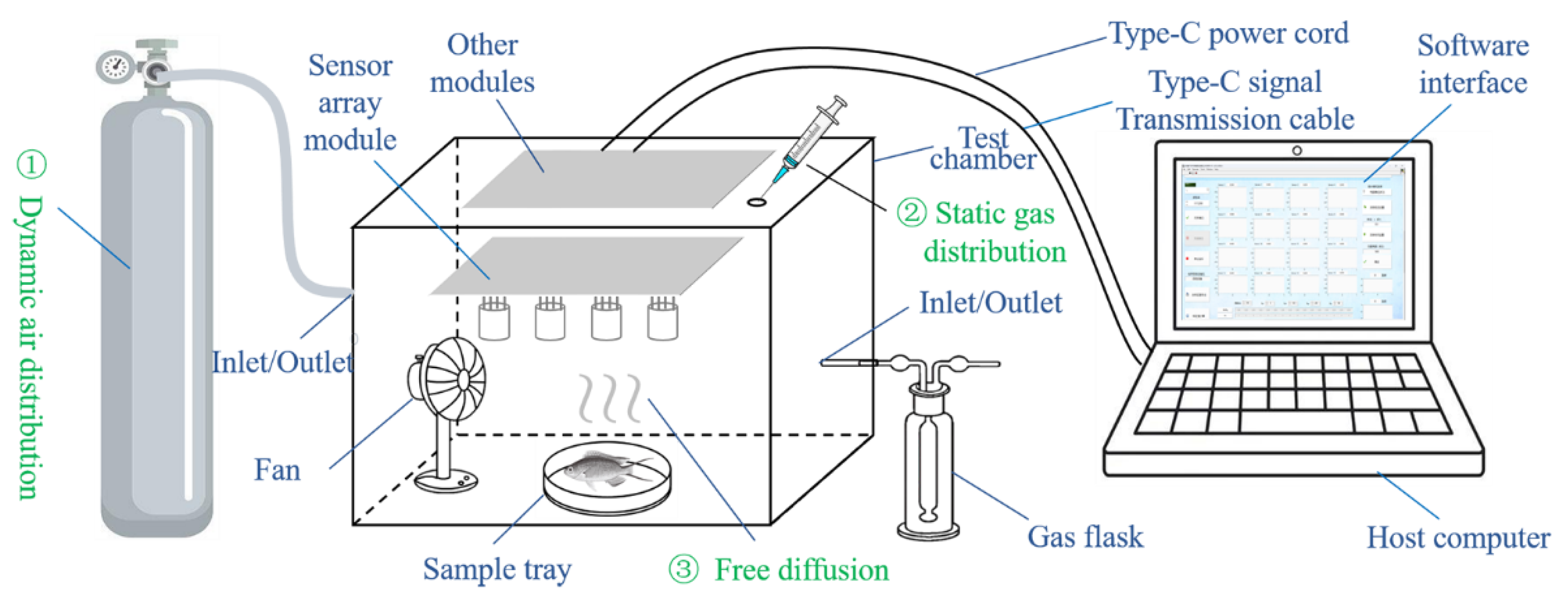
Figure 2.
Gas sensor array system hardware architecture.
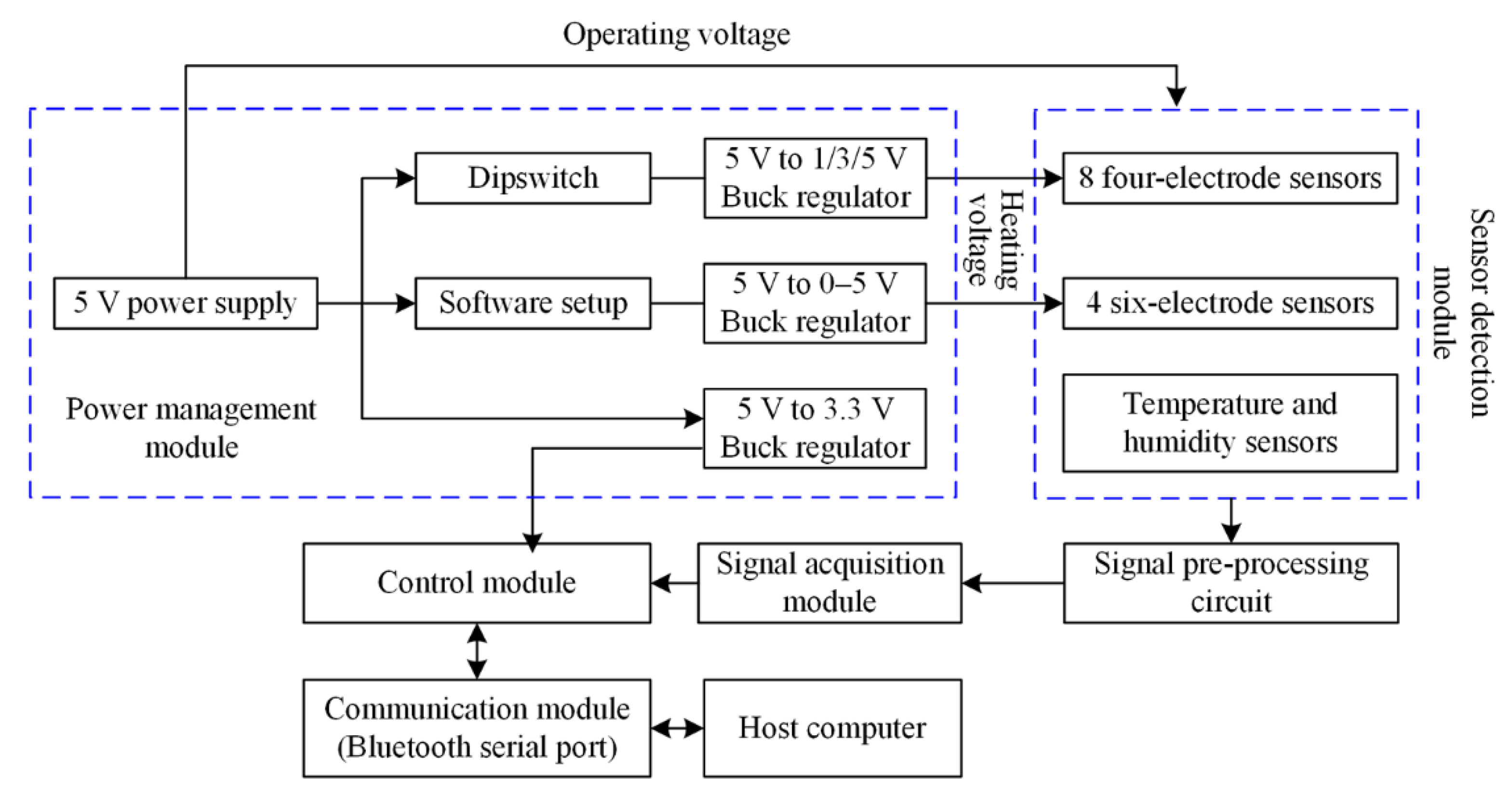
Figure 3.
Response curve of the sensor array.
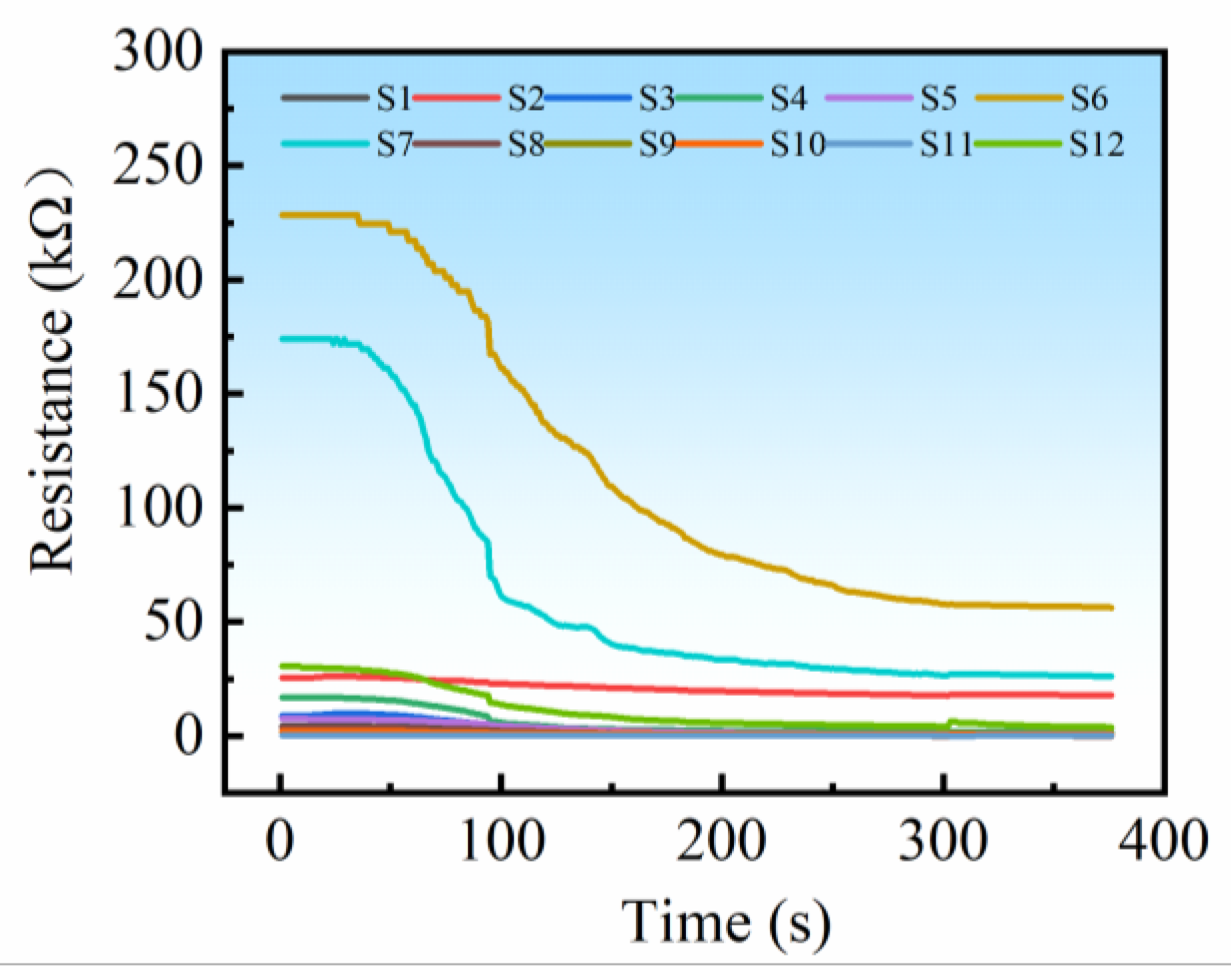
Figure 4.
Changes in appearance and TVB-N content during sample spoilage.
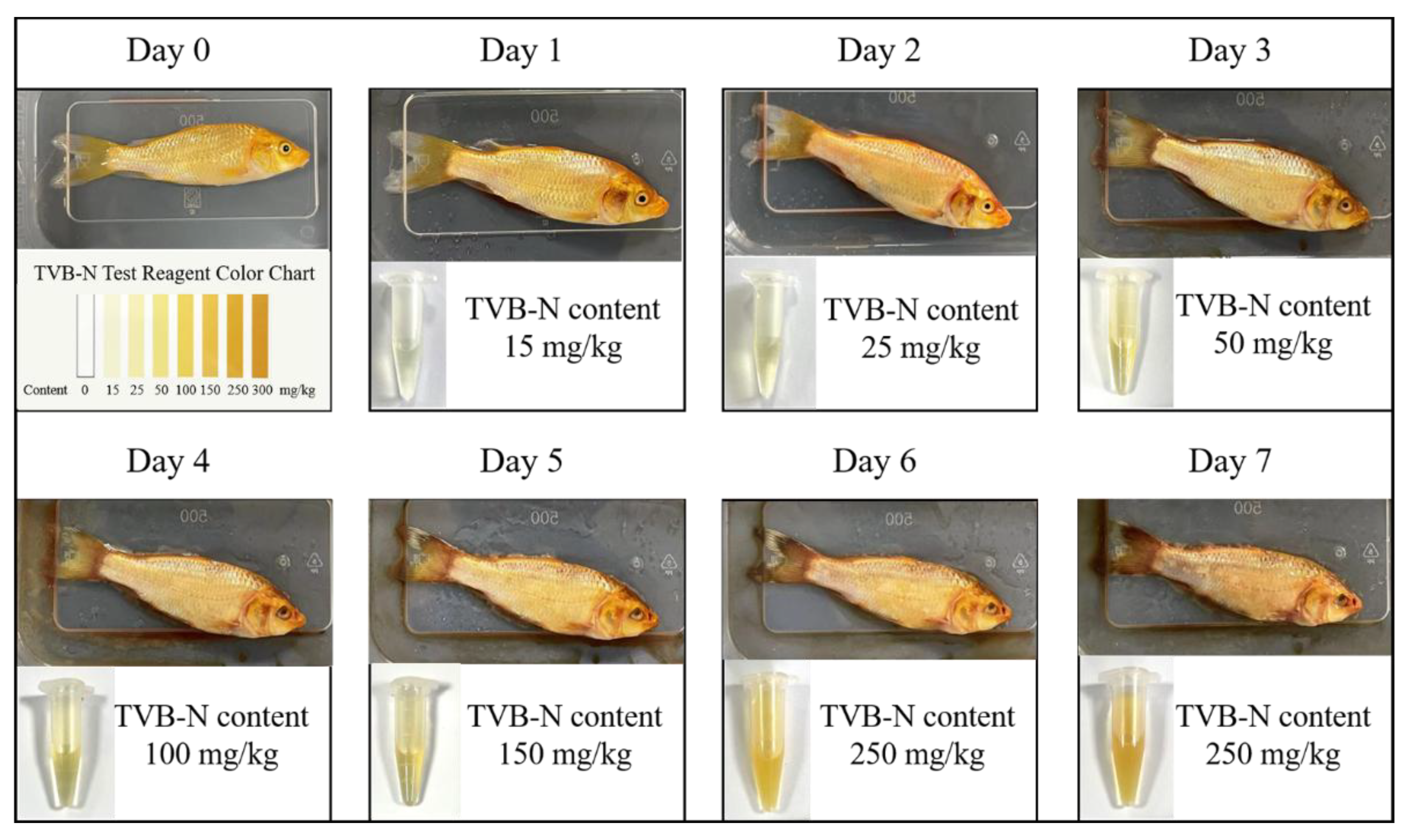
Figure 5.
PCA Analysis of Detection Results from the Selected 12-Sensor Array System.
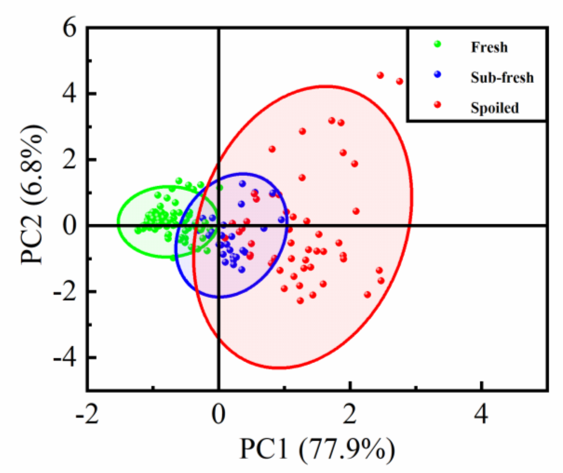
Figure 6.
Classification accuracy of the constructed algorithmic models.
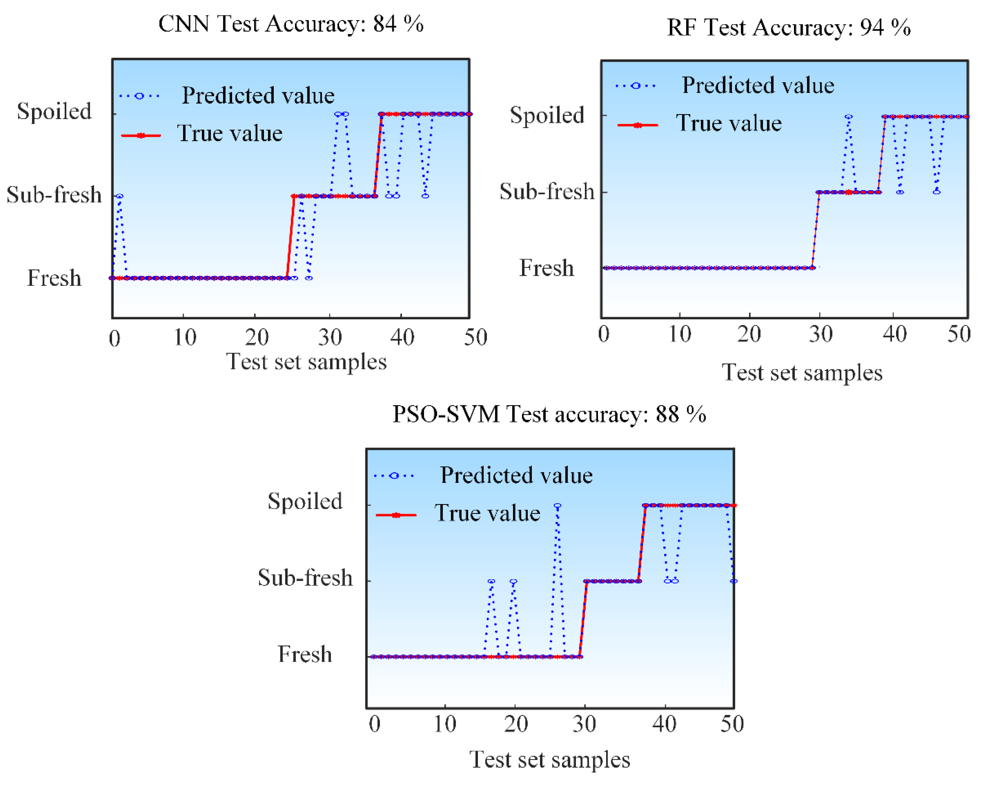
Figure 7.
The confusion matrix of the constructed algorithmic models.
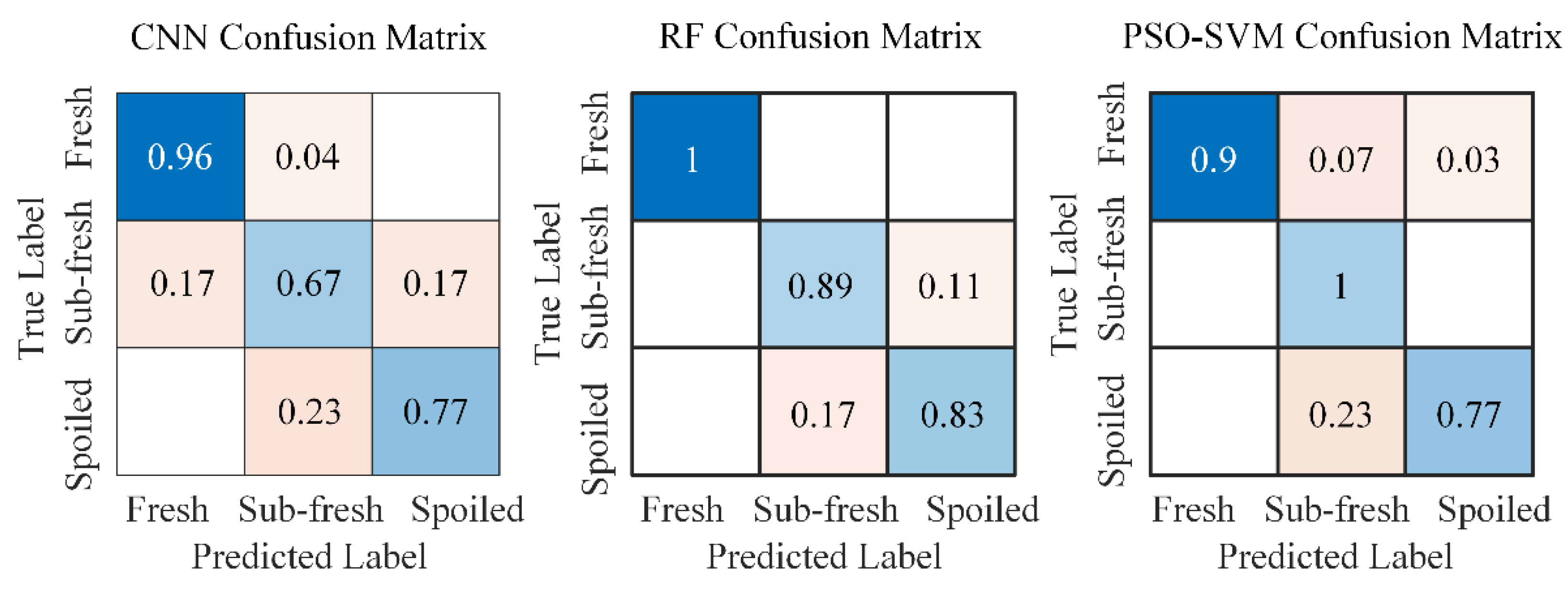
Figure 8.
(a) Correlation analysis between sensor response values and sample spoilage degree; (b) Sensor importance analysis based on RF algorithm.
Figure 8.
(a) Correlation analysis between sensor response values and sample spoilage degree; (b) Sensor importance analysis based on RF algorithm.
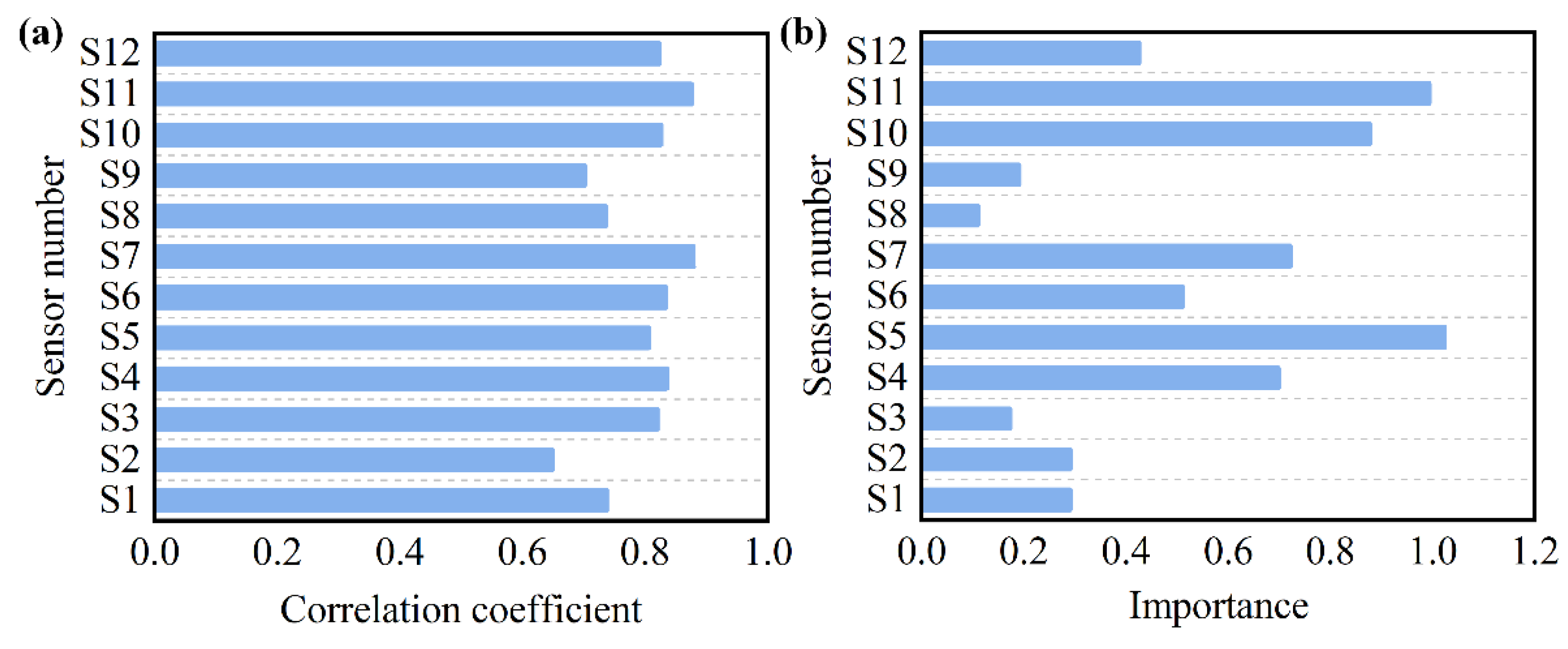
Figure 9.
PCA Analysis of the Optimized Sensor Array System Detection Results.
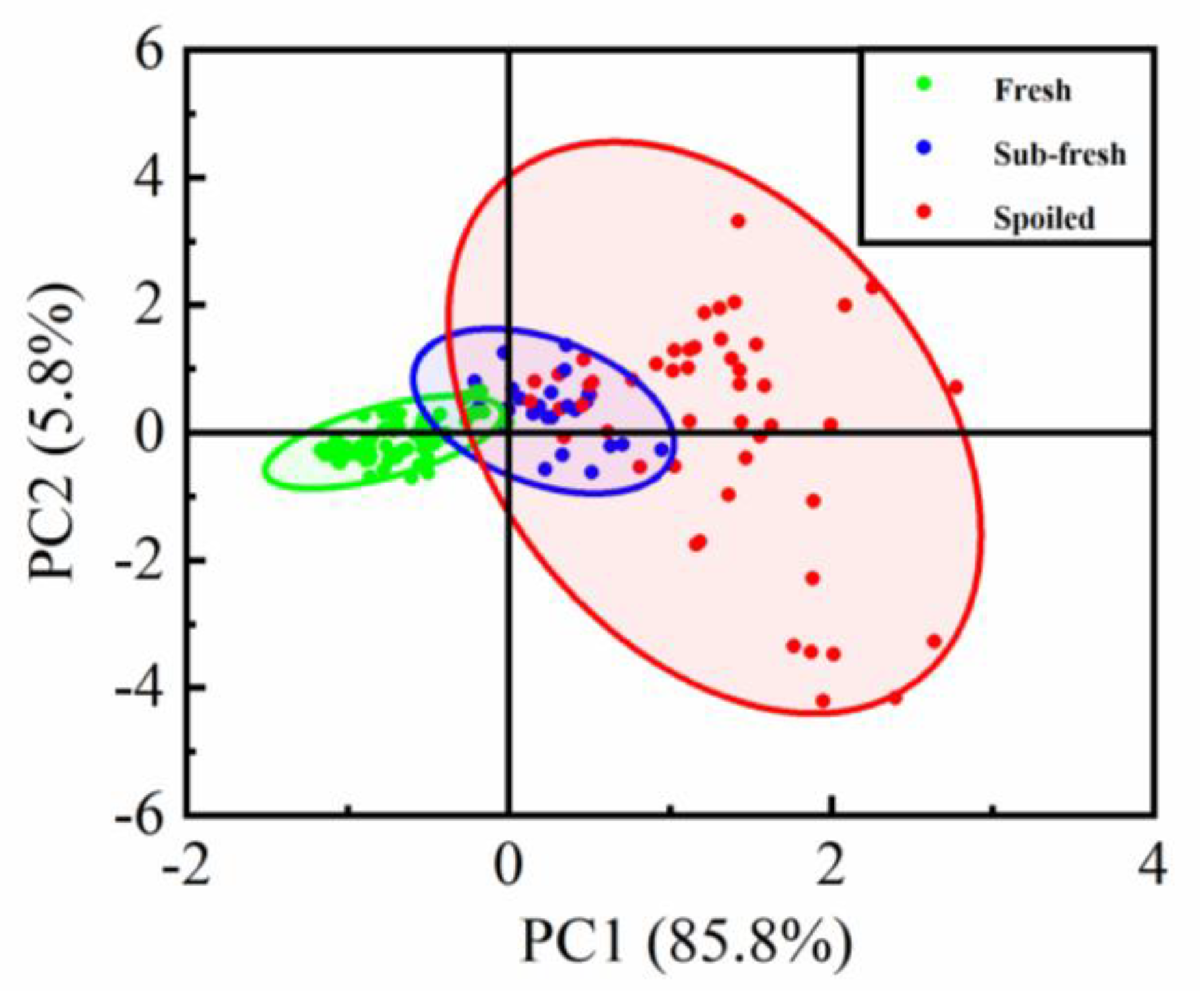
Figure 10.
Classification accuracy of the algorithm model constructed from sample data of the optimized sensor array system: (a) CNN, (b) RF, (c) PSO-SVM; (d) Comparison of prediction accuracy between algorithm models before and after optimization.
Figure 10.
Classification accuracy of the algorithm model constructed from sample data of the optimized sensor array system: (a) CNN, (b) RF, (c) PSO-SVM; (d) Comparison of prediction accuracy between algorithm models before and after optimization.
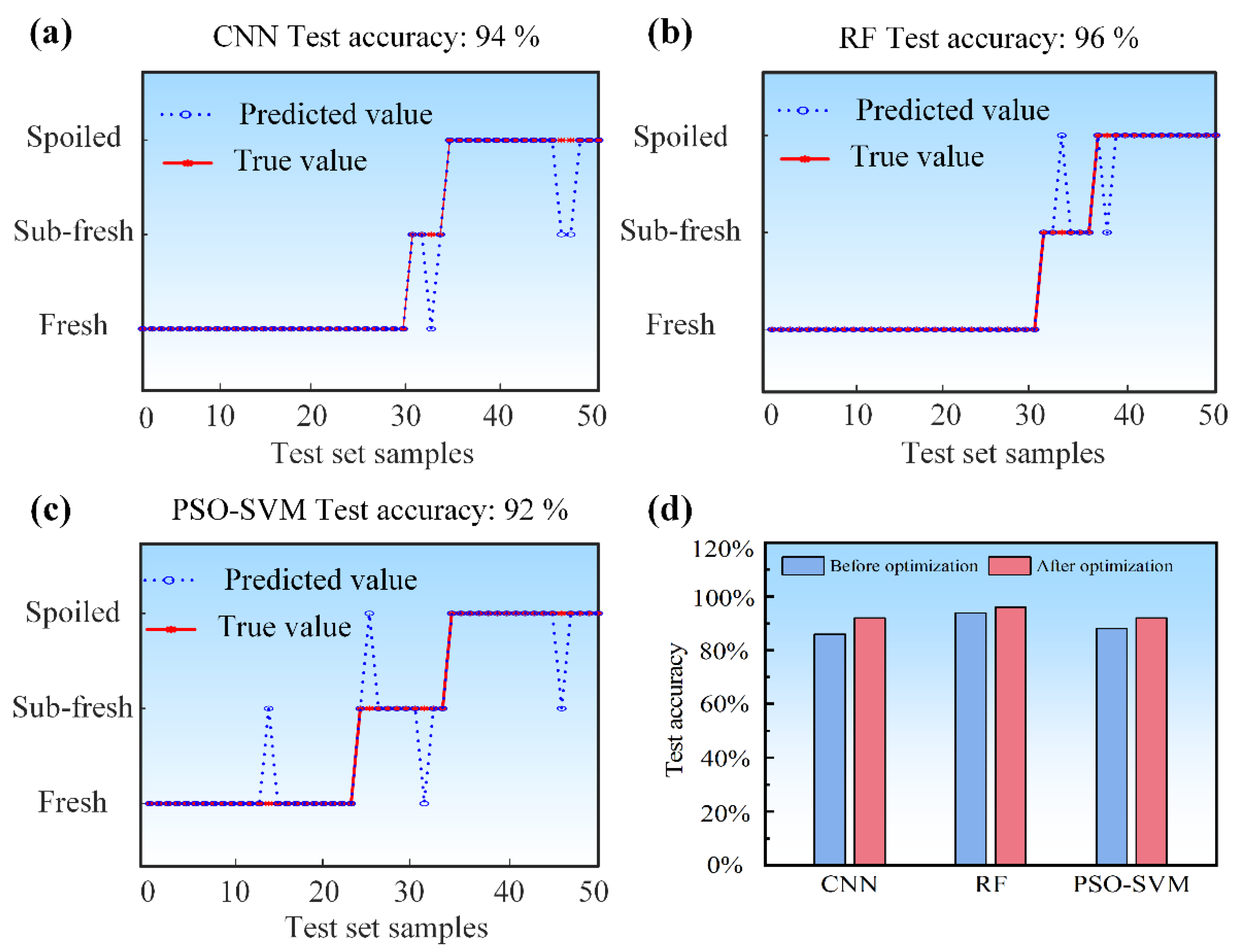

Table 1.
Gas sensor array and its properties.
| Sensor number | Brand | Model | Target gas | Heating voltage (V) |
Detection range (ppm) |
Number of Electrodes |
|---|---|---|---|---|---|---|
| S1 | Figaro | TGS2600 | Hydrogen, Alcohol | 5 | 1~30 | 4 |
| S2 | Figaro | TGS2611 | Methane, Natural gas | 5 | 500~10000 | 4 |
| S3 | Figaro | TGS2602 | Ammonia, Hydrogen sulphide | 5 | 1~30 | 4 |
| S4 | Figaro | TGS2603 | Trimethylamine, Methyl mercaptan | 5 | 1~10 | 4 |
| S5 | Figaro | TGS2620 | Ethanol, Organic solvents | 5 | 50~5000 | 4 |
| S6 | Winsen | WSP2110 | Toluene, Formaldehyde | 5 | 1~50 | 4 |
| S7 | Winsen | WSP7110 | Hydrogen sulfide | 5 | 0~50 | 4 |
| S8 | Winsen | MP702 | Ammonia | 5 | 0~100 | 4 |
| S9 | Self-developed | In2O3 nanocuboids | Triethylamine | 4 | 0.5~100 | 6 |
| S10 | Self-developed | bayberry-like In2O3 | Trimethylamine | 3.5 | 0.5~100 | 6 |
| S11 | Self-developed | flower-like In2O3 | Trimethylamine | 3 | 0.3~100 | 6 |
| S12 | Figaro | TGS 832 | Halogenated hydrocarbons, VOC | 5 | 1~50 | 6 |
Table 2.
Classification of Fish Freshness Status.
| TVB-N content (mg/kg) | Freshness |
|---|---|
| ≤50 | Fresh |
| 50~250 | Sub-fresh |
| ≥250 | Spoiled |
Disclaimer/Publisher’s Note: The statements, opinions and data contained in all publications are solely those of the individual author(s) and contributor(s) and not of MDPI and/or the editor(s). MDPI and/or the editor(s) disclaim responsibility for any injury to people or property resulting from any ideas, methods, instructions or products referred to in the content. |
© 2025 by the authors. Licensee MDPI, Basel, Switzerland. This article is an open access article distributed under the terms and conditions of the Creative Commons Attribution (CC BY) license (http://creativecommons.org/licenses/by/4.0/).
Copyright: This open access article is published under a Creative Commons CC BY 4.0 license, which permit the free download, distribution, and reuse, provided that the author and preprint are cited in any reuse.


