Emergent Dynamics: A Fuzzy Fractional-Order Model Unveiling the Complexities of COVID-19 Transmission

1. Introduction

COVID-19, short for “Coronavirus Disease 2019,” is caused by the novel coronavirus SARS-CoV-2, which was first identified in Wuhan, China, in December 2019. The disease quickly escalated into a global pandemic, affecting millions of people worldwide. COVID-19 primarily spreads through respiratory droplets when an infected person coughs, sneezes, or talks, making it highly contagious. The symptoms of COVID-19 can range from mild to severe and may include fever, cough, shortness of breath, fatigue, muscle or body aches, loss of taste or smell, sore throat, congestion, nausea, vomiting, and diarrhea. Severe cases can lead to pneumonia, acute respiratory distress syndrome (ARDS), organ failure, and death, particularly in older adults and those with underlying health conditions.

Efforts to control the spread of COVID-19 have included widespread testing, contact tracing, quarantine and isolation measures, social distancing, mask-wearing, and vaccination campaigns. Vaccines developed against COVID-19 have played a crucial role in reducing transmission rates and preventing severe illness and death. However, the emergence of new variants of the virus has posed challenges to vaccination efforts and necessitated ongoing surveillance, research, and adaptation of public health strategies. SARS-CoV-2 belongs to the family of coronaviruses, known for causing respiratory illnesses ranging from the common cold to severe acute respiratory syndrome (SARS) and Middle East respiratory syndrome (MERS). The virus primarily spreads through respiratory droplets when an infected person coughs, sneezes, or talks. It can also transmit through contact with contaminated surfaces. COVID-19 presents a wide spectrum of symptoms, ranging from mild respiratory symptoms to severe pneumonia, acute respiratory distress syndrome (ARDS), and multi-organ failure. Common symptoms include fever, cough, shortness of breath, fatigue, muscle or body aches, loss of taste or smell, sore throat, and gastrointestinal issues. However, a significant proportion of infected individuals may remain asymptomatic, posing challenges for disease control and surveillance [1]. Certain factors increase the risk of severe illness and complications from COVID-19, including advanced age, underlying health conditions (such as diabetes, cardiovascular disease, chronic respiratory diseases, and immunosuppression), and socioeconomic disparities. Vulnerable populations, including the elderly, individuals with comorbidities, healthcare workers, and marginalized communities, are at heightened risk of adverse outcomes [2]. Governments, public health agencies, and communities worldwide have implemented various measures to mitigate the spread of COVID-19, including lockdowns, travel restrictions, social distancing, mask mandates, hand hygiene promotion, widespread testing, contact tracing, quarantine, and vaccination campaigns. However, the effectiveness of these interventions depends on factors such as compliance, healthcare infrastructure, and vaccine distribution. The COVID-19 pandemic continues to pose significant challenges to global health, economies, and societies. Efforts to control the spread of the virus, mitigate its impact on vulnerable populations, and accelerate vaccine distribution remain critical priorities. Collaborative research, data sharing, and evidence-based policymaking are essential in navigating this unprecedented crisis and building resilience against future pandemics [3].

The COVID-19 pandemic has spurred an unprecedented level of mathematical modeling and analysis to understand its spread, predict its trajectory, and guide public health responses. Mathematical models serve as invaluable tools for policymakers, epidemiologists, and healthcare professionals in making informed decisions to mitigate the impact of the virus. By integrating data on transmission dynamics, population demographics, interventions, and other factors, these models provide insights into the complex behavior of the pandemic and help evaluate the effectiveness of control measures. Epidemiological models, such as compartmental models (e.g., SIR, SEIR) and agent-based models, simulate the spread of COVID-19 within populations. These models divide the population into compartments based on disease status (susceptible, exposed, infected, recovered) and simulate the flow of individuals between these compartments over time. By incorporating parameters such as transmission rates, incubation periods, and contact patterns, epidemiological models can estimate key epidemiological metrics like the effective reproduction number ($R_0$), epidemic peaks, and the impact of interventions. Mathematical modeling of COVID-19 relies heavily on real-time data sources, including case reports, testing data, hospitalization rates, and mobility patterns. Statistical techniques such as Bayesian inference, time series analysis, and machine learning are employed to analyze and interpret these data, informing model calibration, validation, and forecasting. Data-driven approaches enable researchers to assess the accuracy of model predictions, identify emerging trends, and adapt strategies accordingly [4]. Mathematical models of COVID-19 are subject to various sources of uncertainty, including parameter variability, model structure, and data quality. Sensitivity analysis techniques assess the impact of these uncertainties on model outcomes, helping quantify the robustness of predictions and identify critical factors driving the spread of the virus. Uncertainty quantification facilitates risk assessment, scenario planning, and decision-making under uncertainty [5]. Mathematical modeling plays a crucial role in informing policy decisions related to COVID-19, such as social distancing measures, mask mandates, vaccination strategies, and healthcare resource allocation. Models provide policymakers with evidence-based projections of the potential outcomes of different intervention scenarios, allowing them to weigh trade-offs between public health, economic, and societal considerations. Policy evaluations based on modeling results help optimize resource allocation and minimize the overall burden of the pandemic [6]. Mathematical perspectives offer valuable insights into the dynamics of the COVID-19 pandemic, guiding public health responses and policy decisions. By integrating epidemiological principles, data analytics, and computational techniques, mathematical modeling contributes to our understanding of disease transmission, informs proactive interventions, and enhances preparedness for future health emergencies. Fractional differential equations (FDEs) have emerged as powerful tools for modeling complex dynamical systems exhibiting memory, hereditary properties, and anomalous behaviors. Unlike classical differential equations, which describe systems with integer-order derivatives, FDEs involve derivatives of non-integer order, offering a more flexible framework to capture phenomena with long-range dependencies, non-local effects, and fractal geometries. This introduction provides an overview of fractional calculus and its applications in various scientific disciplines, highlighting recent advancements and key research contributions. Fractional calculus generalizes the concept of differentiation and integration to non-integer orders, enabling the manipulation of functions with fractional exponents. The fractional derivative operator, denoted by $D^{\mathsf{\alpha }}$, where $0<\alpha <1$ or captures the memory and long-range interactions inherent in many physical, biological, and engineering systems. Fractional integrals, fractional differential operators, and fractional differential equations constitute the foundational elements of fractional calculus. FDEs find widespread applications in modeling complex phenomena across various domains, including physics, engineering, finance, biology, and control theory. Examples include anomalous diffusion processes, viscoelastic materials, electromagnetic wave propagation in fractal media, fractional-order circuits, and fractional-order control systems. FDEs offer a versatile framework to describe systems with memory effects, non-local interactions, and fractional dynamics, which are often inadequately captured by classical models [7]. Solving FDEs analytically is often challenging due to the non-local nature of fractional derivatives. Numerical methods, such as fractional finite difference methods, fractional Adams-Bashforth schemes, and fractional spectral methods, play a crucial role in approximating solutions to FDEs. Convergence analysis, stability assessment, and error estimation techniques are essential for ensuring the accuracy and reliability of numerical solutions to fractional differential equations [8]. Recent advancements in fractional calculus have led to novel applications and theoretical developments in various fields. Research efforts focus on refining numerical algorithms, investigating the mathematical properties of fractional operators, exploring fractional-order models for real-world phenomena, and advancing interdisciplinary collaborations. Moreover, the integration of fractional calculus with other mathematical frameworks, such as stochastic processes, dynamical systems theory, and machine learning, opens new avenues for interdisciplinary research and innovation.

Fractional differential equations provide a powerful mathematical framework for modeling complex dynamical systems with memory, non-local interactions, and anomalous behaviors. By extending the classical theory of differentiation to non-integer orders, fractional calculus offers a versatile toolkit for addressing challenges in diverse scientific and engineering disciplines. Continued research and interdisciplinary collaborations are essential for unlocking the full potential of fractional calculus and advancing our understanding of complex phenomena in the natural and engineered world [9]. Epidemic modeling plays a crucial role in understanding the dynamics of infectious diseases and guiding public health interventions. Traditional compartmental models, such as the Susceptible-Infectious-Recovered (SIR) model, assume integer-order derivatives and homogeneous mixing among individuals. However, real-world epidemics often exhibit complex behaviors, including non-Markovian dynamics, long-range interactions, and memory effects. Fractional differential equations (FDEs) offer a flexible framework to capture these complexities, providing a more accurate representation of epidemic spread. This review examines recent advancements in epidemic modeling using fractional calculus and highlights key research contributions in this evolving field. Fractional differential equations extend traditional compartmental models by incorporating fractional-order derivatives to capture memory effects and non-local interactions. Fractional epidemiological models introduce fractional derivatives into the equations governing the dynamics of susceptible, infectious, and recovered populations, allowing for the modeling of complex epidemic behaviors such as long-term memory, sub diffusion, and spatial heterogeneity [10]. Fractional-order epidemiological models offer a more realistic representation of epidemic spread by accounting for phenomena such as sub diffusion, long-range interactions, and heterogeneous mixing patterns. These models can better capture the effects of interventions such as social distancing, quarantine, and vaccination on disease transmission dynamics. Moreover, fractional models enable the study of non-Markovian processes and memory effects, which are prevalent in real-world epidemics [11]. Fractional epidemiological models have been applied to various infectious diseases, including influenza, dengue fever, Ebola, and COVID-19. These models have been used to investigate the impact of interventions, forecast epidemic trajectories, and assess the effectiveness of control measures. Case studies demonstrate the utility of fractional modeling in capturing the complexities of epidemic dynamics and providing insights for public health decision-making [12]. Despite their potential, fractional epidemiological models pose challenges in terms of parameter estimation, model validation, and computational complexity. Future research directions include the development of efficient numerical methods for solving fractional differential equations, the integration of fractional models with data assimilation techniques, and the exploration of multiscale modeling approaches to capture interactions at different spatial and temporal scales [13].

Fractional differential equations offer a promising framework for modeling complex epidemic dynamics, providing a more realistic representation of infectious disease spread compared to traditional compartmental models. By incorporating memory effects, non-local interactions, and heterogeneous mixing patterns, fractional epidemiological models enhance our understanding of epidemic phenomena and inform more effective public health interventions.

1) 

Notations of the concerned parameters

The work has been completed by incorporating twenty parameters, and the details of all parameters are provided in Table 1 with compartments. This version has been modified for better clarity and effectiveness.

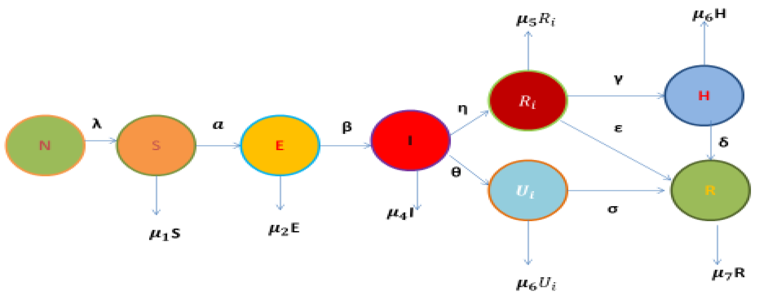
Figure 1. Flow diagram of $\mathit{S}\mathit{E}\mathit{I}{\mathit{R}}_{\mathit{i}}{\mathit{U}}_{\mathit{i}}\mathit{H}\mathit{R}$ model.

Figure 1. Flow diagram of $\mathit{S}\mathit{E}\mathit{I}{\mathit{R}}_{\mathit{i}}{\mathit{U}}_{\mathit{i}}\mathit{H}\mathit{R}$ model.

We construct the differential equation based this dynamic system

$$N=S+E+I+R_i+U_i+H+R\dots \dots \dots \dots \dots \dots \dots \dots \dots \dots ..$$

(1a)

$${\displaystyle \frac{dS}{dt}}=\lambda -\left({\mu }_1+aI\right)\dots \dots \dots \dots \dots \dots \dots \dots \dots \dots \dots \dots \dots \dots \dots \dots ..$$

(1b)

$${\displaystyle \frac{dE}{dt}}=aSI-\left({\mu }_2+\beta \right)E\dots \dots \dots \dots \dots \dots \dots \dots \dots \dots \dots \dots \dots \dots \dots .$$

(1c)

$${\displaystyle \frac{dI}{dt}}=\beta E-\left(d+{\mu }_3+\theta +\eta \right)I\dots \dots \dots \dots \dots \dots \dots \dots \dots \dots \dots \dots$$

(1d)

$${\displaystyle \frac{d{R}_I}{dt}}=\eta I-\left(\mathsf{\gamma }+\mathsf{\epsilon }+{\mu }_4+d\right)R_I\dots \dots \dots \dots \dots \dots \dots \dots \dots \dots .$$

(1f)

$${\displaystyle \frac{d{\mathrm{U}}_{\mathrm{I}}}{dt}}=\theta \mathrm{I}-\left(\mathsf{\mu }+\mathsf{\sigma }+{\mu }_5\right){\mathrm{U}}_{\mathrm{I}}\dots \dots \dots \dots \dots \dots \dots \dots \dots \dots .\dots$$

(1g)

$${\displaystyle \frac{dH}{dt}}=\gamma R_I-\left({\mu }_6+\mu +\delta \right)H\dots \dots \dots \dots \dots \dots \dots \dots \dots \dots \dots ..$$

(1h)

$${\displaystyle \frac{dR}{dt}}=\sigma {\mathrm{U}}_{\mathrm{I}}+\epsilon R_I+\delta H-{\mu }_{7}R\dots \dots \dots \dots \dots \dots \dots \dots \dots \dots ..$$

(1i)

As the mathematical epidemic problem will be taken as the initial condition by written below.$S\left(0\right)>0,E\left(0\right)>0,I\left(0\right)>0,R_i\left(0\right)>0,U_i\left(0\right)>0,H\left(0\right)>0,R\left(0\right)>0.$

In our study, we aim to mathematically analyses the infection system of 2019-nCoV (novel coronavirus) using advanced techniques. Specifically, we employ the fuzzy Laplace transform based on Adomian decomposition to obtain numerical results. This approach offers valuable insights into the dynamical structures governing the physical behavior of 2019-nCoV [14]. To model the outbreak of the coronavirus, we formulate a system of seven equations representing nonlinear fractional order differential equations (FODEs). These equations depict various stages of the infection process, including Susceptible (S), Exposed (E), Infected (I), Reported ($R_i$), Unreported ($U_i$), and Recovered (R). Each equation captures the interactions and transitions between these compartments, providing a comprehensive framework for understanding the spread and control of the virus [15]. Our methodology builds upon previous research on infectious disease modelling and fractional calculus. By applying the fuzzy Laplace transform and Adomian decomposition, we extend the analytical capabilities to address the unique characteristics of 2019-nCoV. The numerical results obtained from this approach offer valuable insights into the complex dynamics of the epidemic, aiding in the development of effective control strategies and public health interventions [16]. This study contributes to the growing body of literature on mathematical modelling of infectious diseases and provides a novel perspective on the dynamics of 2019-nCoV. The insights gained from this research have implications for epidemic forecasting, healthcare resource allocation, and policy decision-making in response to emerging infectious threats [17].

$$D_t^{\alpha }S\left(t\right)=\lambda -{(\mathrm{\mu }}_1+a)S=\lambda -{\mathrm{\mu }}_{1}S-aS\dots \dots \dots \dots \dots \dots \dots \dots \dots \dots \dots \dots \dots \dots .$$

2(a)

$$D_t^{\alpha }E\left(t\right)=aSI-\left({\mathrm{\mu }}_2+\beta \right)E=aSI-{\mathrm{\mu }}_{2}E-\beta E\dots \dots \dots \dots \dots \dots \dots \dots \dots \dots \dots ....$$

2(b)

$$D_t^{\alpha }I\left(t\right)=\beta E-\left(d+{\mu }_3+\theta +\eta \right)I=\beta E-dI-{\mu }_{3}I-\theta I-\eta I\dots \dots \dots \dots \dots .$$

2(c)

$$D_t^{\alpha }{R}_i\left(t\right)=\eta I-\left(\gamma +{\mu }_5+\epsilon \right)R_i=\eta I-{\gamma R}_i-{\mu }_5{R}_i-\epsilon R_i\dots \dots \dots \dots \dots \dots .\dots .$$

2(d)

$$D_t^{\alpha }{\mathrm{U}}_{\mathrm{i}}\left(t\right)=\theta \mathrm{I}-\left({\mathsf{\mu }}_4+\mathsf{\sigma }\right){\mathrm{U}}_{\mathrm{i}}=\theta \mathrm{I}-{{\mathsf{\mu }}_4\mathrm{U}}_{\mathrm{i}}-\mathsf{\sigma }{\mathrm{U}}_{\mathrm{i}}\dots \dots \dots \dots \dots \dots \dots \dots \dots \dots ..\dots .$$

2(e)

$$D_t^{\alpha }H\left(t\right)=\gamma R_i-\left(\mu +\delta +d\right)H=\gamma R_i-\mu H-\delta H-dH\dots \dots \dots \dots \dots ...........$$

2(f)

$$D_t^{\alpha }R\left(t\right)=\sigma {\mathrm{U}}_{\mathrm{i}}+\epsilon R_i+\delta H-dR\dots \dots \dots \dots \dots \dots \dots \dots .\dots \dots \dots \dots \dots \dots .\dots \dots ..$$

2(g)

In recent years, there has been a significant expansion of modern calculus and differential equations (DEs) to encompass fuzzy calculus and fractional-order differential equations (FODEs), respectively. This progression has further extended to fuzzy FODEs, broadening the scope of mathematical modelling to accommodate uncertainty and imprecision [18]. Researchers have extensively studied FODEs and fuzzy integral equations to establish theories regarding the existence and uniqueness of solutions. However, when dealing with fuzzy FODEs, the computation of precise solutions becomes particularly challenging. Consequently, mathematicians have dedicated considerable efforts to develop various solution methods, including perturbation methods, integral transform methods, and spectral techniques. Additionally, stability analysis of fuzzy DEs has been conducted by some researchers, providing valuable insights into the behavior of these complex systems [19]. In this study, we focus on investigating a model with a fuzzy fractional-order derivative, introducing uncertainty into the initial data. Specifically, we consider the formulation [20]. In this study, we focus on investigating a model with a fuzzy fractional-order derivative, introducing uncertainty into the initial data. Specifically, we consider the formulation:

$$D_{fuzzy}^{\alpha }y\left(t\right)=f(t,y\left(t\right))$$

Where $0<\alpha \le 1,$and $D_{fuzzy}^{\alpha }$ represents the fuzzy fractional-order derivative.

This investigation builds upon the foundation of fuzzy calculus and fractional calculus, aiming to address the challenges posed by uncertainty in differential equations. By incorporating fuzzy concepts into fractional-order derivatives, we seek to provide a more comprehensive framework for modelling real-world phenomena affected by imprecise or uncertain data [21].

$$D_t^{\alpha }S\left(t\right)=\tilde{\lambda }-(\widetilde{{\mathrm{\mu }}_1}+\tilde{a})S=\lambda -\widetilde{{\mathrm{\mu }}_1}S-\tilde{a}S\dots \dots \dots \dots \dots \dots \dots \dots \dots ..$$

3(a)

$$D_t^{\alpha }E\left(t\right)=\tilde{a}SI-\left(\widetilde{{\mathrm{\mu }}_2}+\tilde{\beta }\right)E=\tilde{a}SI-\widetilde{{\mathrm{\mu }}_2}E-\tilde{\beta }E\dots \dots \dots \dots \dots \dots ...$$

3(b)

$$D_t^{\alpha }I\left(t\right)=\tilde{\beta }E-\left(\tilde{d}+\widetilde{{\mu }_3}+\tilde{\theta }+\tilde{\eta }\right)I=\tilde{\beta }E-\tilde{d}I-\widetilde{{\mu }_3}I-\tilde{\theta }I-\tilde{\eta }I\dots$$

3(c)

$$D_t^{\alpha }{R}_i\left(t\right)=\tilde{\eta }I-\left(\tilde{\gamma }+\widetilde{{\mu }_5}+\tilde{\epsilon }\right)R_i=\tilde{\eta }I-{\tilde{\gamma }R}_i-\widetilde{{\mu }_5}{R}_i-\tilde{\epsilon }{R}_i\dots \dots \dots$$

3(d)

$$D_t^{\alpha }{\mathrm{U}}_{\mathrm{i}}\left(t\right)=\tilde{\theta }\mathrm{I}-\left(\widetilde{{\mathsf{\mu }}_4}+\tilde{\mathsf{\sigma }}\right){\mathrm{U}}_{\mathrm{i}}=\tilde{\theta }\mathrm{I}-{\widetilde{{\mathsf{\mu }}_4}\mathrm{U}}_{\mathrm{i}}-\tilde{\mathsf{\sigma }}{\mathrm{U}}_{\mathrm{i}}\dots \dots \dots \dots \dots \dots \dots .$$

3(e)

$$D_t^{\alpha }H\left(t\right)=\tilde{\gamma }{R}_i-\left(\tilde{\mu }+\tilde{\delta }+\tilde{d}\right)H=\tilde{\gamma }{R}_i-\tilde{\mu }H-\tilde{\delta }H-\tilde{d}H\dots \dots \dots$$

3(f)

$$D_t^{\alpha }R\left(t\right)=\tilde{\sigma }{\mathrm{U}}_{\mathrm{i}}+\tilde{\epsilon }{R}_i+\tilde{\delta }H-\tilde{d}R\dots \dots \dots \dots \dots \dots \dots \dots \dots ..\dots \dots .$$

3(g)

Associated to fuzzy initial condition, for α ∈ [0, 1],

$$\tilde{\mathit{S}}\left(0,\mathit{\alpha }\right)=(\underset{\_}{\mathit{S}}\left(0,\mathit{\alpha }\right),\overline{\mathit{S}}\left(0,\mathit{\alpha }\right)),\tilde{\mathit{E}}\left(0,\mathit{\alpha }\right)=\left(\underset{\_}{\mathit{E}}\left(0,\mathit{\alpha }\right),\overline{\mathit{E}}\left(0,\mathit{\alpha }\right)\right),$$

$$\tilde{\mathit{I}}\left(0,\mathit{\alpha }\right)=\left(\underset{\_}{\mathit{I}}\left(0,\mathit{\alpha }\right),\overline{\mathit{I}}\left(0,\mathit{\alpha }\right)\right),\widetilde{{\mathit{R}}_{\mathit{i}}}\left(0,\mathit{\alpha }\right)=\left(\underset{\_}{{\mathit{R}}_{\mathit{i}}}\left(0,\mathit{\alpha }\right),\overline{{\mathit{R}}_{\mathit{i}}}\left(0,\mathit{\alpha }\right)\right),$$

$$\widetilde{{\mathbf{U}}_{\mathit{i}}}\left(0,\mathit{\alpha }\right)=\left(\underset{\_}{{\mathbf{U}}_{\mathbf{i}}}\left(0,\mathit{\alpha }\right),\overline{{\mathbf{U}}_{\mathbf{i}}}\left(0,\mathit{\alpha }\right)\right),\tilde{\mathit{H}}\left(0,\mathit{\alpha }\right)=(\underset{\_}{\mathit{H}}\left(0,\mathit{\alpha }\right),\overline{\mathit{H}}\left(0,\mathit{\alpha }\right)),$$

$$\tilde{\mathit{R}}\left(0,\mathit{\alpha }\right)=\left(\underset{\_}{\mathit{R}}\left(0,\mathit{\alpha }\right),\overline{\mathit{R}}\left(0,\mathit{\alpha }\right)\right)$$

In response to the current uncertain situation surrounding the COVID-19 pandemic, we were inspired to develop a novel model for coronavirus infection dynamics utilizing concepts from fuzzy fractional calculus. Our motivation stems from the need to better understand and characterize the complex behavior of viral spread, particularly in scenarios where traditional models may fall short in capturing the inherent uncertainty and variability [22]. The proposed model not only incorporates fuzzy fractional calculus but also aims to enhance the representation of the physical behavior exhibited by the COVID-19 infection system. By integrating fuzzy logic and fractional calculus, we strive to create a more realistic framework that closely aligns with the dynamic properties of RNA viruses, such as COVID-19 [23]. Our model emphasizes the dynamic interactions between various compartments of the infection system, including susceptible, exposed, infected, reported, unreported, and recovered individuals. Through the incorporation of fuzzy fractional calculus, we account for uncertainties in parameters and initial conditions, thereby improving the model’s ability to reflect real-world complexities [24,25].

By leveraging insights from fuzzy mathematics and fractional calculus, our proposed model offers a more nuanced understanding of COVID-19 transmission dynamics. It provides a valuable tool for researchers and policymakers to assess the effectiveness of interventions, forecast epidemic trajectories, and inform public health strategies in the face of evolving uncertainties [26,27].

2) 

Preliminaries:

This section provides an overview of fundamental concepts relevant to fuzzy fractional calculus, which serve as the foundation for the subsequent discussions.

3a) Fuzzy Set Theory: Fuzzy set theory, introduced by Zadeh in 1965, extends classical set theory to accommodate degrees of membership rather than strict binary distinctions. Fuzzy sets are characterized by membership functions that assign a degree of membership to each element of the set [28]

$$A=\left\{\left(x,{\mathrm{\mu }}_A\left(x\right)\right)\right|x\in X,0<{\mathrm{\mu }}_A\left(x\right)\le 1\}$$

This expression denotes that A consists of ordered pairs $\left(x,{\mu }_A\left(x\right)\right),$where $x$ belong to universal of discourse $X$, and ${\mu }_A\left(x\right)$represents the degree of membership of $x$ in the fuzzy set A. The degree of membership ${\mu }_A\left(x\right)$varies between 0 to 1, inclusively, reflecting the extent to which $x$ belong to $A$. This mathematical representation encapsulates the fuzzy nature of the set A, allowing for the modelling of uncertainty and vagueness in data.

3b) Fractional Calculus: Fractional calculus deals with derivatives and integrals of non-integer orders. It provides a mathematical framework for analyzing systems with fractional dynamics, offering insights into phenomena such as anomalous diffusion and viscoelastic behavior [29].

Fractional calculus is a branch of mathematics that deals with derivatives and integrals of non-integer orders. It extends the concepts of traditional calculus to include fractional derivatives and integrals, enabling the analysis of systems with fractional dynamics. Fractional calculus has found applications in various fields such as physics, engineering, biology, and finance. It allows for the modelling of phenomena exhibiting complex behavior, including anomalous diffusion, viscoelasticity, and fractals [32]. A fractional derivative of order α of a function $f\left(x\right)$, denoted by $D^{\alpha }f\left(x\right)$, is define as

$D^{\alpha }f\left(x\right)={\displaystyle \frac{1}{\mathit{\Gamma }\left(\mathit{n}-\alpha \right)}}\left[{\displaystyle \frac{d^n}{\mathit{d}{\mathit{x}}^{\mathit{n}}}}\underset{\mathit{a}}{\overset{\mathit{x}}{\int }}{\left(\mathit{x}-\mathit{t}\right)}^{\mathit{n}-\alpha -1}\mathit{f}\left(\mathit{t}\right)\mathit{d}\mathit{t}\right]$ where $n-1<\alpha <n$ and $n$ is the smallest integer greater than $\alpha$, and $\Gamma$ is the gamma function [30,31].

3c) Fuzzy Fractional Calculus: Fuzzy fractional calculus combines fuzzy logic and fractional calculus, allowing for the analysis of systems with uncertain or imprecise data using fractional-order operators with fuzzy parameters [33]. Fuzzy fractional calculus is a mathematical framework that combines concepts from fuzzy set theory and fractional calculus. It allows for the analysis of systems with uncertain or imprecise data using fractional-order operators with fuzzy parameters. A fuzzy fractional derivative of order $\alpha$ for a fuzzy-valued function $f\left(x\right)$, denoted by $D_{fuzzy}^{\alpha }f\left(x\right)$, can be defined using fuzzy set theory and fractional calculus principles. One common approach is to extend the fractional derivative definition to incorporate fuzzy membership functions. A possible expression for the fuzzy fractional derivative is:

$$D_{fuzzy}^{\alpha }f\left(x\right)={\displaystyle \frac{1}{\mathit{\Gamma }\left(\mathit{n}-\alpha \right)}}\left[{\displaystyle \frac{d^n}{\mathit{d}{\mathit{x}}^{\mathit{n}}}}\underset{\mathit{a}}{\overset{\mathit{x}}{\int }}{\left(\mathit{x}-\mathit{t}\right)}^{\mathit{n}-\alpha -1}\mathrm{\mu }\left(\mathit{t}\right)\mathit{f}\left(\mathit{t}\right)\mathit{d}\mathit{t}\right]$$

where $n-1<\alpha <n,$ n is the smallest integer greater than $\alpha ,\mu \left(t\right)$ is the fuzzy membership function, and $\Gamma$ is the gamma function [34,35].

3d) Fuzzy Fractional Differential Equations (FFDEs): FFDEs are differential equations involving fuzzy fractional derivatives. These equations provide a framework for modelling systems exhibiting both fractional dynamics and fuzzy uncertainty. Fuzzy fractional differential equations (FFDEs) are differential equations that combine the concepts of fuzzy set theory and fractional calculus. They are used to model dynamic systems where the rate of change of a variable is described by a fractional derivative and the parameters or initial conditions involve uncertainty captured by fuzzy logic.

A general form of a fuzzy fractional differential equation can be represented as:

$$D_{fuzzy}^{\alpha }f\left(x\right)=f\left(t,y\left(t\right)\right)$$

Where:

• $D_{fuzzy}^{\alpha }f\left(x\right)$represents the fuzzy fractional derivative operator,
• $y\left(t\right)$ is the unknown function of time, $f\left(t,y\left(t\right)\right)$ is a function describing the relationship between y and its derivatives with respect to t, and $0<\alpha \le 1$ denotes the order of the fractional derivative.
• The fuzzy fractional derivative $D_{fuzzy}^{\alpha }y\left(t\right)$ incorporates both fuzzy set theory and fractional calculus, allowing for the modelling of systems with uncertain or imprecise dynamics [36,37,38].

3e) Fuzzy Number:

A fuzzy number is a generalization of a crisp (traditional) number, which represents a precise value, to a range of values with associated degrees of membership. In other words, a fuzzy number expresses uncertainty or vagueness regarding the exact value of a quantity. A fuzzy number A is typically defined by a membership function ${\mu }_A\left(x\right)$ that assigns a degree of membership to each real number $x$ within a specified interval. The membership function ${\mu }_A\left(x\right)$. indicates the degree to which x belongs to the fuzzy number A, with values ranging from 0 (not a member) to 1 (fully a member). Mathematically, the membership function ${\mu }_A\left(x\right)$ satisfies the following properties:

Non-negativity: ${\mu }_A\left(x\right)\ge 0$for all $x$

Normalization: $Su{p}_x$ ${\mu }_A\left(x\right)=1,$where sup denotes the supremum.

3f) Fuzziness: The membership function ${\mu }_A\left(x\right)$can take any value between 0 and 1, inclusively as mathematical represented${\mu }_A\left(x\right):[\mathrm{a},\mathrm{b}]-\to \left[01\right]$. An expression for a fuzzy number A can be written as: $A=\left\{\left(x,{\mu }_A\left(x\right)\right)\right|x\in [a,b]\},$[42] Where [a,b] is the interval over which the fuzzy number is defined, and ${\mu }_A\left(x\right)$is the membership function indicating the degree of membership of each x in the interval. Fuzzy numbers are useful in representing imprecise or uncertain data in various fields, including decision making, control systems, and optimization.

3e) Fuzzy –level set: Fuzzy level sets are a generalization of traditional level sets to accommodate uncertainty or ambiguity in defining boundaries between regions in images or data. They provide a flexible framework for capturing gradual transitions and uncertain distinctions between objects or features. Let Ω denote the domain of interest, and consider a fuzzy set A defined over Ω. The fuzzy level set $\varphi \left(x\right)$ is defined as a scalar function that represents the degree to which each point $x$in $\Omega$ belongs to the fuzzy set $A$. Formally, the fuzzy level set $\varphi \left(x\right)$ is defined by its membership function ${\mu }_{\varphi }\left(x\right)$ which assigns a degree of membership to each point $x$ in Ω which assigns a degree of membership to each point x in indicating the extent to which $x$lies within the boundary of the fuzzy set $A$.

The mathematical expression for a fuzzy level set $\varphi \left(x\right)$ can be represented as $\varphi \left(x\right)$ = ${\mu }_{\varphi }\left(x\right)$. Where ${\mu }_{\varphi }\left(x\right)$ is the membership function of the fuzzy level set indicating the degree of membership of each point $xin$Ω. $A_{\alpha }=\left\{x\in \mathsf{\Omega }\right|{\mu }_A\left(x\right)\ge \alpha \}$ which yields a crisp set representation of the fuzzy boundary. [39,40,41]

Boundedness: The boundedness of a fuzzy number $\tilde{A}$ is inherent in its definition within a closed interval [a,b] $supp\left(\tilde{A}\right)=\left\{x\in \mathbb{R}\right|{\mu }_A\left(x\right)\ge 0\}\subseteq [a,b],a,b\in \mathbb{R},a<b$ [43].

Convexity: The convexity of the membership function ${\mu }_A\left(x\right)$ensures that it monotonically increases from 0 to 1 within the interval [a,b], implying that for any

$x_1,x_2$ such that $x_1<x_2,{\mathrm{\mu }}_A\left(x_1\right)\le {\mathrm{\mu }}_A\left(x_2\right)$[44]

3f) Hausdorff Distance

The Hausdorff distance is a measure of similarity between two sets of points in a metric space. It quantifies how far apart two sets are from each other by considering the maximum distance of a point in one set to the closest point in the other set. Let A and B be two subsets of a metric space X. The Hausdorff distance $d_H(A,B)$ between A and B is define as:

$$d_H\left(A,B\right)=\mathrm{m}\mathrm{a}\mathrm{x}\{{\mathrm{s}\mathrm{u}\mathrm{p}}_{\mathrm{a}\in \mathrm{A}}in{f}_{b\in B}d\left(a,b\right),{\mathrm{s}\mathrm{u}\mathrm{p}}_{\mathrm{b}\in \mathrm{B}}In{f}_{a\in A}d\left(b,a\right)$$

3g) H-difference:

Let A and B be two fuzzy numbers. The Hukuhara difference (or H-difference) of $\tilde{A}$ and $\tilde{B}$ is the fuzzy number $\tilde{C}$ such that $\tilde{A}=\tilde{B}\oplus \tilde{C}$ where $\oplus$ denotes Minkowski addition of fuzzy numbers.

In terms of α-cuts, it is given by $\widetilde{(A}\oplus {\tilde{B})}_{\alpha }=\left[{\underset{\_}{A}}_{\alpha }-{\underset{\_}{B}}_{\alpha },{\overline{A}}_{\alpha }-B_{\alpha }\right],{\forall }_{\alpha }\in \left[0,1\right].$

3h) Fuzzy Mapping:

A fuzzy mapping, also known as a fuzzy function, is a generalization of a traditional (crisp) mapping that allows for the representation of uncertain or vague relationships between elements of two sets. In a fuzzy mapping, each element of the domain set is associated with a fuzzy set of values in the range set, reflecting the degree of membership of each element in the output set.

Let X and Y be two sets, and consider a fuzzy mapping f from X to Y. A fuzzy mapping f assigns to each element x in the domain set X a fuzzy set of values in the range set Y, denoted as $f\left(x\right)$.

$$f:X\to f\left(Y\right)$$

Where $f\left(Y\right)$is represented represents the set of all subsets of Y. For each $x\in X$ the fuzzy set $f\left(x\right)$ characterizes the uncertain relationship between x and the elements of Y.

$$f\left(x\right)=\left\{\left(y,{\mathrm{\mu }}_{f\left(x\right)}\left(y\right)\right)\right|y\in Y\}$$

Where ${\mu }_{f\left(x\right)}\left(y\right)$ is the membership function that assigns a degree of membership to each $y$ in $Y$ for the element $x$ in $X$.

The fuzzy mapping $f$ allows for the representation of imprecise or uncertain relationships between real numbers and linguistic terms, capturing the gradual transitions between different degrees of membership.

3i) Riemann-Liouville fractional integral:

The Riemann-Liouville fractional integral is a generalization of the classical integral to non-integer orders. It is defined by a convolution integral involving the original function and a weight function, typically expressed as a power function.

Let $f\left(x\right)$ be a real valued function defined on the interval [a,b], and let $\alpha >0$be a real number. The Riemann-Liouville fractional integral of order $\alpha$ of $f\left(x\right),$ denoted by $I^{\alpha }f\left(x\right)$ , is defined as:

$${(\mathit{I}}_{\mathit{a}}^{\alpha }\mathit{f})\left(\mathit{x}\right)={\displaystyle \frac{1}{\mathit{\Gamma }\left(\alpha \right)}}\underset{\alpha }{\overset{\mathit{x}}{\int }}{\left(\mathit{x}-\mathit{t}\right)}^{\alpha -1}\mathit{f}\left(\mathit{t}\right)\mathit{d}\mathit{t},\alpha ,\mathit{t}\in \left(0,\mathrm{\infty }\right)x>a$$

Where $\mathit{\Gamma }\left(\alpha \right)$is the gamma function.

For a fuzzy-valued function $\mathit{\varphi }\left(\mathit{t}\right),$with parameteric form

$${{[\mathit{I}}_{\mathit{a}}^{\alpha }\mathit{\varphi }\left(\mathit{t}\right)]}_{\mathit{P}}={\mathit{I}}_{\mathit{a}}^{\alpha }\underset{\_}{{\mathit{\varphi }}_{\mathit{p}}}\left(\mathit{t}\right),{\mathit{I}}_{\mathit{a}}^{\alpha }\overline{{\mathit{\varphi }}_{\mathit{p}}}\left(\mathit{t}\right)],0\le \mathit{p}\le 1,$$

$${\mathit{I}}_{\mathit{a}}^{\alpha }\underset{\_}{{\mathit{\varphi }}_{\mathit{p}}}\left(\mathit{t}\right)={\displaystyle \frac{1}{\mathit{\Gamma }\left(\alpha \right)}}\underset{\alpha }{\overset{\mathit{x}}{\int }}{\left(\mathit{x}-\mathit{s}\right)}^{\alpha -1}\underset{\_}{{\mathit{\varphi }}_{\mathit{p}}}\left(\mathit{s}\right)\mathit{d}\mathit{s},\alpha ,\mathit{t}\in (0,\mathrm{\infty })$$

$${\mathit{I}}_{\mathit{a}}^{\alpha }\overline{{\mathit{\varphi }}_{\mathit{p}}}\left(\mathit{t}\right)={\displaystyle \frac{1}{\mathit{\Gamma }\left(\alpha \right)}}\underset{\alpha }{\overset{\mathit{x}}{\int }}{\left(\mathit{x}-\mathit{s}\right)}^{\alpha -1}\overline{{\mathit{\varphi }}_{\mathit{p}}}\left(\mathit{s}\right)\mathit{d}\mathit{s},\alpha ,\mathit{t}\in (0,\mathrm{\infty })$$

3j) Fixed point theory:

Let’s consider the modified right-hand side of the fuzzy fractional model (2) using fixed point theory to discuss its existence and uniqueness. Here’s a formulation of the modified model:

$$D^{\alpha }u\left(t\right)=F\left(t,u\left(t\right),\mathrm{\mu }\right),$$

Where $F:\left[a,b\right]\chi X\chi Y\to X$ is a mapping defined on a closed interval [a, b] with $X$ and $Y$ being Banach spaces. The parameter $\mu$ represents the fuzzy parameters that capture uncertainty or imprecision.

To discuss the existence and uniqueness of solutions to this model, we can utilize fixed point theory. Fixed point theory provides conditions under which a mapping has a unique fixed point, which in turn can be related to the existence and uniqueness of solutions to the differential equation [52,53,54].

3k) Fuzzy Fractional Caputo’s Derivative

The fuzzy fractional Caputo’s derivative is a generalization of the traditional Caputo’s derivative to accommodate fractional-order operators with fuzzy parameters. It extends the concept of fuzzy fractional calculus to describe the dynamics of systems with uncertain or imprecise fractional orders.

Mathematical Expression:

The fuzzy fractional Caputo’s derivative of a function $y\left(t\right)$ is defined as:

$${\mathit{D}}_{\mathit{f}\mathit{u}\mathit{z}\mathit{z}\mathit{y}}^{\alpha }\mathit{y}\left(\mathit{t}\right)={\displaystyle \frac{1}{\mathit{\Gamma }\left(1-\alpha \right)}}\left[\underset{\alpha }{\overset{\mathit{t}}{\int }}{\left(\mathit{t}-\mathit{\tau }\right)}^{-\alpha }\mathrm{\mu }\left(\mathit{\tau }\right){\mathit{y}}^{\prime }\left(\mathit{\tau }\right)\mathit{d}\mathit{\tau }\right]$$

Where $0<\alpha \le 1$ is the fractional order, $\Gamma$ is the gamma function, $\mathit{\mu }\left(\mathit{\tau }\right)$is the fuzzy membership function indicating the degree of membership of $\tau$ in a fuzzy set, and $y^{\prime }\left(\tau \right)$ denotes the derivative of $y\left(\tau \right)$ with respect to $\tau$ [45,46,47].

3l) Upper and lower bound in $\mathit{\alpha }$ cut

Let $\tilde{x}$ be a fuzzy number with membership function ${\mu }_{\tilde{x}}$ : $R-\to \left[01\right]$. For given $\alpha \in \left(01\right]$, the $\alpha -cut$of $\tilde{x}$ is defined as:

$${\left[\tilde{x}\right]}_{\alpha }=\left\{x\in R\right|{\mu }_{\tilde{x}}\left(x\right)\ge \alpha \},0<\alpha \le 1.$$

This $\alpha$cut is always a closed and bounded interval: ${\left[\tilde{x}\right]}_{\alpha }=\left[\underset{\_}{x}\left(\alpha \right),\overline{x}\left(\alpha \right)\right]$

$\underset{\_}{x}\left(\alpha \right)$is the fuzzy lower bound (left endpoint) — a non-decreasing function of α

$\overline{x}\left(\alpha \right)$ is the fuzzy upper bound (right endpoint) — a non-increasing function of α

3) 

Fuzzy Laplace Transform

The fuzzy Laplace transform is a mathematical tool used to analyses and solve differential equations involving fuzzy initial conditions or parameters. It extends the classical Laplace transform to accommodate uncertainty or imprecision present in the system.

Given a function $f\left(t\right)$ with fuzzy initial conditions or parameters, the fuzzy Laplace transform $F\left(s\right)$ is defined as:

$$F\left(s\right)=\underset{0}{\overset{\mathrm{\infty }}{\int }}{\mathit{e}}^{-\mathit{s}\mathit{t}}\mathrm{\mu }\left(\mathit{\tau }\right)\mathit{f}\left(\mathit{t}\right)\mathit{d}\mathit{t}.$$

where:

• $\mu \left(t\right)$ is the membership function representing the fuzziness of the initial conditions or parameter
• $s$ is the complex variable in the Laplace domain, and t is the time variable, The fuzzy Laplace transform $F\left(s\right)$ provides a representation of the function $f\left(t\right)$ in the Laplace domain, considering the uncertainty encapsulated by the membership function $\mu \left(t\right)$ [48,50]

For $0\le r\le 1,$the parametric form of $\mathit{\varphi }\left(\mathit{\chi }\right)$ is represented by

$$\underset{0}{\overset{\mathrm{\infty }}{\int }}\mathit{f}\left(\mathit{\chi },\mathit{r}\right).{\mathit{e}}^{-\mathit{s}\mathit{\chi }}\mathit{d}\mathit{\chi }=\left[\underset{0}{\overset{\mathrm{\infty }}{\int }}\underset{\_}{\mathit{f}}\left(\mathit{\chi },\mathit{r}\right).{\mathit{e}}^{-\mathit{s}\mathit{\chi }}\mathit{d}\mathit{\chi },\underset{0}{\overset{\mathrm{\infty }}{\int }}\overline{\mathit{f}}\left(\mathit{\chi },\mathit{r}\right).{\mathit{e}}^{-\mathit{s}\mathit{\chi }}\mathit{d}\mathit{\chi },\right]$$

$$L\left[\mathit{f}\left(\mathit{\chi },\mathit{r}\right)\right]=[\mathit{L}\underset{\_}{\mathit{f}}\left(\mathit{\chi },\mathit{r}\right),\mathit{L}\overline{\mathit{f}}\left(\mathit{\chi },\mathit{r}\right)]$$

Theorem 1 

[51]. $f\in C^F[0,b]\cap L^F[0,b]$ then for $0\le p\le 1$ and $0<\beta \le 1$, the Laplace transform of fuzzy fractional derivative in Caputo’s sense is given by

$$L\left[{\left({\mathit{D}}^{\beta }\mathit{f}\left(\mathit{t}\right)\right)}_{\mathit{p}}\right]={\mathit{S}}^{\beta }\mathit{L}\left[\mathit{f}\left(\mathit{t}\right)\right]-{\mathit{S}}^{\beta -1}\mathit{L}\left[\mathit{f}\left(0\right)\right]$$

4) 

Main results

In the following section, the existence and uniqueness of solution to the subsequent fuzzy

fractional model is discussed; and we provide the procedure for finding a semi analytic

solution of model by using fuzzy Laplace transform.

5) 

Existence and uniqueness

In this section, by the use of fixed point theory, the existence and uniqueness of the subsequent fuzzy fractional model is discussed. Consider the right-hand sides of model (2):

$$\begin{gathered} \mathit{A}\left(\mathit{t},\mathit{S}\left(\mathit{t}\right),\mathit{E}\left(\mathit{t}\right),\mathit{I}\left(\mathit{t}\right),{\mathit{R}}_{\mathit{i}}\left(\mathit{t}\right),{\mathit{U}}_{\mathit{i}}\left(\mathit{t}\right),\mathit{H}\left(\mathit{t}\right),\mathit{R}\left(\mathit{t}\right)\right)=\tilde{\mathit{\lambda }}-(\widetilde{{\mathrm{\mu }}_1}+\tilde{\mathit{a}})\mathit{S}=\mathit{\lambda }-\widetilde{{\mathrm{\mu }}_1}\mathit{S}-\tilde{\mathit{a}}\mathit{S} \\ \mathit{B}\left(\mathit{t},\mathit{S}\left(\mathit{t}\right),\mathit{E}\left(\mathit{t}\right),\mathit{I}\left(\mathit{t}\right),{\mathit{R}}_{\mathit{i}}\left(\mathit{t}\right),{\mathit{U}}_{\mathit{i}}\left(\mathit{t}\right),\mathit{H}\left(\mathit{t}\right),\mathit{R}\left(\mathit{t}\right)\right)=\tilde{\mathit{a}}\mathit{S}\mathit{I}-\left(\widetilde{{\mathrm{\mu }}_2}+\tilde{\mathit{\beta }}\right)\mathit{E}=\tilde{\mathit{a}}\mathit{S}\mathit{I}-\widetilde{{\mathrm{\mu }}_2}\mathit{E}-\tilde{\mathit{\beta }}\mathit{E} \\ \mathit{C}\left(\mathit{t},\mathit{S}\left(\mathit{t}\right),\mathit{E}\left(\mathit{t}\right),\mathit{I}\left(\mathit{t}\right),{\mathit{R}}_{\mathit{i}}\left(\mathit{t}\right),{\mathit{U}}_{\mathit{i}}\left(\mathit{t}\right),\mathit{H}\left(\mathit{t}\right),\mathit{R}\left(\mathit{t}\right)\right)=\tilde{\mathit{\beta }}\mathit{E}-\left(\tilde{\mathit{d}}+\widetilde{{\mathit{\mu }}_3}+\tilde{\mathit{\theta }}+\tilde{\mathit{\eta }}\right)\mathit{I}=\tilde{\mathit{\beta }}\mathit{E}-\tilde{\mathit{d}}\mathit{I}-\widetilde{{\mathit{\mu }}_3}\mathit{I}-\tilde{\mathit{\theta }}\mathit{I}-\tilde{\mathit{\eta }}\mathit{I} \\ \mathit{D}\left(\mathit{t},\mathit{S}\left(\mathit{t}\right),\mathit{E}\left(\mathit{t}\right),\mathit{I}\left(\mathit{t}\right),{\mathit{R}}_{\mathit{i}}\left(\mathit{t}\right),{\mathit{U}}_{\mathit{i}}\left(\mathit{t}\right),\mathit{H}\left(\mathit{t}\right),\mathit{R}\left(\mathit{t}\right)\right)=\tilde{\mathit{\eta }}\mathit{I}-\left(\tilde{\mathit{\gamma }}+\widetilde{{\mathit{\mu }}_5}+\tilde{\mathit{\epsilon }}\right){\mathit{R}}_{\mathit{i}}=\tilde{\mathit{\eta }}\mathit{I}-{\tilde{\mathit{\gamma }}\mathit{R}}_{\mathit{i}}-\widetilde{{\mathit{\mu }}_5}{\mathit{R}}_{\mathit{i}}-\tilde{\mathit{\epsilon }}{\mathit{R}}_{\mathit{i}} \\ \mathit{E}\left(\mathit{t},\mathit{S}\left(\mathit{t}\right),\mathit{E}\left(\mathit{t}\right),\mathit{I}\left(\mathit{t}\right),{\mathit{R}}_{\mathit{i}}\left(\mathit{t}\right),{\mathit{U}}_{\mathit{i}}\left(\mathit{t}\right),\mathit{H}\left(\mathit{t}\right),\mathit{R}\left(\mathit{t}\right)\right)=\tilde{\mathit{\theta }}\mathbf{I}-\left(\widetilde{{\mathsf{\mu }}_4}+\tilde{\mathsf{\sigma }}\right){\mathbf{U}}_{\mathbf{i}}=\tilde{\mathit{\theta }}\mathbf{I}-{\widetilde{{\mathsf{\mu }}_4}\mathbf{U}}_{\mathbf{i}}-\tilde{\mathsf{\sigma }}{\mathbf{U}}_{\mathbf{i}} \\ \mathit{F}\left(\mathit{t},\mathit{S}\left(\mathit{t}\right),\mathit{E}\left(\mathit{t}\right),\mathit{I}\left(\mathit{t}\right),{\mathit{R}}_{\mathit{i}}\left(\mathit{t}\right),{\mathit{U}}_{\mathit{i}}\left(\mathit{t}\right),\mathit{H}\left(\mathit{t}\right),\mathit{R}\left(\mathit{t}\right)\right)=\tilde{\mathit{\gamma }}{\mathit{R}}_{\mathit{i}}-\left(\tilde{\mathit{\mu }}+\tilde{\mathit{\delta }}+\tilde{\mathit{d}}\right)\mathit{H}= \\ \tilde{\mathit{\gamma }}{\mathit{R}}_{\mathit{i}}-\tilde{\mathit{\mu }}\mathit{H}-\tilde{\mathit{\delta }}\mathit{H}-\tilde{\mathit{d}}\mathit{H} \\ \mathit{G}\left(\mathit{t},\mathit{S}\left(\mathit{t}\right),\mathit{E}\left(\mathit{t}\right),\mathit{I}\left(\mathit{t}\right),{\mathit{R}}_{\mathit{i}}\left(\mathit{t}\right),{\mathit{U}}_{\mathit{i}}\left(\mathit{t}\right),\mathit{H}\left(\mathit{t}\right),\mathit{R}\left(\mathit{t}\right)\right)=\tilde{\mathit{\sigma }}{\mathbf{U}}_{\mathbf{i}}+\tilde{\mathit{\epsilon }}{\mathit{R}}_{\mathit{i}}+\tilde{\mathit{\delta }}\mathit{H}-\tilde{\mathit{d}}\mathit{R} \end{gathered}$$

Where A, B, C, D, E, F and G are fuzzy function. Thus, for $0<\alpha \le 1$ the given model (2) can be written as

$$\left\{\begin{array}{c}{\mathit{D}}_{\mathit{t}}^{\mathit{\alpha }}S\left(\mathit{t}\right)=A\left(\mathit{t},\mathit{S}\left(\mathit{t}\right),\mathit{E}\left(\mathit{t}\right),\mathit{I}\left(\mathit{t}\right),{\mathit{R}}_{\mathit{i}}\left(\mathit{t}\right),{\mathit{U}}_{\mathit{i}}\left(\mathit{t}\right),\mathit{H}\left(\mathit{t}\right),\mathit{R}\left(\mathit{t}\right)\right)\dots \dots .\mathbf{4}\left(\mathit{a}\right)\\ {\mathit{D}}_{\mathit{t}}^{\mathit{\alpha }}E\left(\mathit{t}\right)=B\left(\mathit{t},\mathit{S}\left(\mathit{t}\right),\mathit{E}\left(\mathit{t}\right),\mathit{I}\left(\mathit{t}\right),{\mathit{R}}_{\mathit{i}}\left(\mathit{t}\right),{\mathit{U}}_{\mathit{i}}\left(\mathit{t}\right),\mathit{H}\left(\mathit{t}\right),\mathit{R}\left(\mathit{t}\right)\right)\dots \dots \mathbf{4}\left(\mathit{b}\right)\\ {\mathit{D}}_{\mathit{t}}^{\mathit{\alpha }}I\left(\mathit{t}\right)=C\left(\mathit{t},\mathit{S}\left(\mathit{t}\right),\mathit{E}\left(\mathit{t}\right),\mathit{I}\left(\mathit{t}\right),{\mathit{R}}_{\mathit{i}}\left(\mathit{t}\right),{\mathit{U}}_{\mathit{i}}\left(\mathit{t}\right),\mathit{H}\left(\mathit{t}\right),\mathit{R}\left(\mathit{t}\right)\right)\dots \dots ..\mathbf{4}\left(\mathit{c}\right)\\ {\mathit{D}}_{\mathit{t}}^{\mathit{\alpha }}{\mathit{R}}_{\mathit{i}}\left(\mathit{t}\right)=\left(\mathit{t},\mathit{S}\left(\mathit{t}\right),\mathit{E}\left(\mathit{t}\right),\mathit{I}\left(\mathit{t}\right),{\mathit{R}}_{\mathit{i}}\left(\mathit{t}\right),{\mathit{U}}_{\mathit{i}}\left(\mathit{t}\right),\mathit{H}\left(\mathit{t}\right),\mathit{R}\left(\mathit{t}\right)\right)\dots \dots \dots \mathbf{4}\left(\mathit{d}\right)\\ {\mathit{D}}_{\mathit{t}}^{\mathit{\alpha }}{\mathbf{U}}_{\mathbf{i}}\left(\mathit{t}\right)=E\left(\mathit{t},\mathit{S}\left(\mathit{t}\right),\mathit{E}\left(\mathit{t}\right),\mathit{I}\left(\mathit{t}\right),{\mathit{R}}_{\mathit{i}}\left(\mathit{t}\right),{\mathit{U}}_{\mathit{i}}\left(\mathit{t}\right),\mathit{H}\left(\mathit{t}\right),\mathit{R}\left(\mathit{t}\right)\right)\dots .\mathbf{4}\left(\mathit{e}\right)\\ {\mathit{D}}_{\mathit{t}}^{\mathit{\alpha }}H\left(\mathit{t}\right)=F\left(\mathit{t},\mathit{S}\left(\mathit{t}\right),\mathit{E}\left(\mathit{t}\right),\mathit{I}\left(\mathit{t}\right),{\mathit{R}}_{\mathit{i}}\left(\mathit{t}\right),{\mathit{U}}_{\mathit{i}}\left(\mathit{t}\right),\mathit{H}\left(\mathit{t}\right),\mathit{R}\left(\mathit{t}\right)\right)\dots \dots .\dots .\mathbf{4}\left(\mathit{f}\right)\\ {\mathit{D}}_{\mathit{t}}^{\mathit{\alpha }}R\left(\mathit{t}\right)=G\left(\mathit{t},\mathit{S}\left(\mathit{t}\right),\mathit{E}\left(\mathit{t}\right),\mathit{I}\left(\mathit{t}\right),{\mathit{R}}_{\mathit{i}}\left(\mathit{t}\right),{\mathit{U}}_{\mathit{i}}\left(\mathit{t}\right),\mathit{H}\left(\mathit{t}\right),\mathit{R}\left(\mathit{t}\right)\right)\dots \dots .\mathbf{4}\left(\mathit{g}\right)\end{array}\right.$$

with fuzzy initial conditions:

$$\begin{gathered} \tilde{\mathit{S}}\left(0,\mathit{\alpha }\right)=(\underset{\_}{\mathit{S}}\left(0,\mathit{\alpha }\right),\overline{\mathit{S}}\left(0,\mathit{\alpha }\right)),\tilde{\mathit{E}}\left(0,\mathit{\alpha }\right)=\left(\underset{\_}{\mathit{E}}\left(0,\mathit{\alpha }\right),\overline{\mathit{E}}\left(0,\mathit{\alpha }\right)\right), \\ \tilde{\mathit{I}}\left(0,\mathit{\alpha }\right)=\left(\underset{\_}{\mathit{I}}\left(0,\mathit{\alpha }\right),\overline{\mathit{I}}\left(0,\mathit{\alpha }\right)\right),\widetilde{{\mathit{R}}_{\mathit{i}}}\left(0,\mathit{\alpha }\right)=\left(\underset{\_}{{\mathit{R}}_{\mathit{i}}}\left(0,\mathit{\alpha }\right),\overline{{\mathit{R}}_{\mathit{i}}}\left(0,\mathit{\alpha }\right)\right), \\ \widetilde{{\mathbf{U}}_{\mathit{i}}}\left(0,\mathit{\alpha }\right)=\left(\underset{\_}{{\mathbf{U}}_{\mathbf{i}}}\left(0,\mathit{\alpha }\right),\overline{{\mathbf{U}}_{\mathbf{i}}}\left(0,\mathit{\alpha }\right)\right),\tilde{\mathit{H}}\left(0,\mathit{\alpha }\right)=(\underset{\_}{\mathit{H}}\left(0,\mathit{\alpha }\right),\overline{\mathit{H}}\left(0,\mathit{\alpha }\right)), \\ \tilde{\mathit{R}}\left(0,\mathit{\alpha }\right)=\left(\underset{\_}{\mathit{R}}\left(0,\mathit{\alpha }\right),\overline{\mathit{R}}\left(0,\mathit{\alpha }\right)\right). \end{gathered}$$

Now applying fuzzy fractional integral $I^r$and using initial conditions, we get

$$\left\{\begin{array}{c}{\mathit{S}}_{\mathit{n}}\left(\mathit{t}\right)=\tilde{\mathit{S}}\left(0,\mathit{\alpha }\right)+{\displaystyle \frac{1}{\mathit{\Gamma }\left(\mathit{\gamma }\right)}}\underset{0}{\overset{\mathit{t}}{\int }}{\left(\mathit{t}-\mathit{\Delta }\right)}^{\mathit{\gamma }-1}A\left(\mathit{t},\mathit{S}\left(\mathit{t}\right),\mathit{E}\left(\mathit{t}\right),\mathit{I}\left(\mathit{t}\right),{\mathit{R}}_{\mathit{i}}\left(\mathit{t}\right),{\mathit{U}}_{\mathit{i}}\left(\mathit{t}\right),\mathit{H}\left(\mathit{t}\right),\mathit{R}\left(\mathit{t}\right)\right)\dots .\mathbf{5}(\mathit{a})\\ {\mathit{E}}_{\mathit{n}}\left(\mathit{t}\right)=\tilde{\mathit{E}}\left(0,\mathit{\alpha }\right)+{\displaystyle \frac{1}{\mathit{\Gamma }\left(\mathit{\gamma }\right)}}\underset{0}{\overset{\mathit{t}}{\int }}{\left(\mathit{t}-\mathit{\Delta }\right)}^{\mathit{\gamma }-1}A\left(\mathit{t},\mathit{S}\left(\mathit{t}\right),\mathit{E}\left(\mathit{t}\right),\mathit{I}\left(\mathit{t}\right),{\mathit{R}}_{\mathit{i}}\left(\mathit{t}\right),{\mathit{U}}_{\mathit{i}}\left(\mathit{t}\right),\mathit{H}\left(\mathit{t}\right),\mathit{R}\left(\mathit{t}\right)\right)\dots .\mathbf{5}(\mathit{b})\\ {\mathit{I}}_{\mathit{n}}\left(\mathit{t}\right)=\tilde{\mathit{I}}\left(0,\mathit{\alpha }\right)+{\displaystyle \frac{1}{\mathit{\Gamma }\left(\mathit{\gamma }\right)}}\underset{0}{\overset{\mathit{t}}{\int }}{\left(\mathit{t}-\mathit{\Delta }\right)}^{\mathit{\gamma }-1}A\left(\mathit{t},\mathit{S}\left(\mathit{t}\right),\mathit{E}\left(\mathit{t}\right),\mathit{I}\left(\mathit{t}\right),{\mathit{R}}_{\mathit{i}}\left(\mathit{t}\right),{\mathit{U}}_{\mathit{i}}\left(\mathit{t}\right),\mathit{H}\left(\mathit{t}\right),\mathit{R}\left(\mathit{t}\right)\right)\dots .\mathbf{5}(\mathit{c})\\ {\mathit{R}}_{{\mathit{i}}_{\mathit{n}}}\left(\mathit{t}\right)=\widetilde{{\mathit{R}}_{\mathit{i}}}\left(0,\mathit{\alpha }\right)+{\displaystyle \frac{1}{\mathit{\Gamma }\left(\mathit{\gamma }\right)}}\underset{0}{\overset{\mathit{t}}{\int }}{\left(\mathit{t}-\mathit{\Delta }\right)}^{\mathit{\gamma }-1}A\left(\mathit{t},\mathit{S}\left(\mathit{t}\right),\mathit{E}\left(\mathit{t}\right),\mathit{I}\left(\mathit{t}\right),{\mathit{R}}_{\mathit{i}}\left(\mathit{t}\right),{\mathit{U}}_{\mathit{i}}\left(\mathit{t}\right),\mathit{H}\left(\mathit{t}\right),\mathit{R}\left(\mathit{t}\right)\right)\dots .\mathbf{5}(\mathit{d})\\ {{\mathit{U}}_{\mathit{i}}}_{\mathit{n}}\left(\mathit{t}\right)=\widetilde{{\mathit{U}}_{\mathit{i}}}\left(0,\mathit{\alpha }\right)+{\displaystyle \frac{1}{\mathit{\Gamma }\left(\mathit{\gamma }\right)}}\underset{0}{\overset{\mathit{t}}{\int }}{\left(\mathit{t}-\mathit{\Delta }\right)}^{\mathit{\gamma }-1}A\left(\mathit{t},\mathit{S}\left(\mathit{t}\right),\mathit{E}\left(\mathit{t}\right),\mathit{I}\left(\mathit{t}\right),{\mathit{R}}_{\mathit{i}}\left(\mathit{t}\right),{\mathit{U}}_{\mathit{i}}\left(\mathit{t}\right),\mathit{H}\left(\mathit{t}\right),\mathit{R}\left(\mathit{t}\right)\right)\dots .\mathbf{5}(\mathit{e})\\ {\mathit{H}}_{\mathit{n}}\left(\mathit{t}\right)=\tilde{\mathit{H}}\left(0,\mathit{\alpha }\right)+{\displaystyle \frac{1}{\mathit{\Gamma }\left(\mathit{\gamma }\right)}}\underset{0}{\overset{\mathit{t}}{\int }}{\left(\mathit{t}-\mathit{\Delta }\right)}^{\mathit{\gamma }-1}A\left(\mathit{t},\mathit{S}\left(\mathit{t}\right),\mathit{E}\left(\mathit{t}\right),\mathit{I}\left(\mathit{t}\right),{\mathit{R}}_{\mathit{i}}\left(\mathit{t}\right),{\mathit{U}}_{\mathit{i}}\left(\mathit{t}\right),\mathit{H}\left(\mathit{t}\right),\mathit{R}\left(\mathit{t}\right)\right)\dots .\mathbf{5}(\mathit{f})\\ {\mathit{R}}_{\mathit{n}}\left(\mathit{t}\right)=\tilde{\mathit{R}}\left(0,\mathit{\alpha }\right)+{\displaystyle \frac{1}{\mathit{\Gamma }\left(\mathit{\gamma }\right)}}\underset{0}{\overset{\mathit{t}}{\int }}{\left(\mathit{t}-\mathit{\Delta }\right)}^{\mathit{\gamma }-1}A\left(\mathit{t},\mathit{S}\left(\mathit{t}\right),\mathit{E}\left(\mathit{t}\right),\mathit{I}\left(\mathit{t}\right),{\mathit{R}}_{\mathit{i}}\left(\mathit{t}\right),{\mathit{U}}_{\mathit{i}}\left(\mathit{t}\right),\mathit{H}\left(\mathit{t}\right),\mathit{R}\left(\mathit{t}\right)\right)\dots .\mathbf{5}(\mathit{g})\end{array}\right.$$

Let us define a Banach space as $\mathcal{B}={\mathcal{B}}_1\mathit{\chi }{\mathcal{B}}_2\mathit{\chi }{\mathcal{B}}_3\mathit{\chi }{\mathcal{B}}_4\mathit{\chi }{\mathcal{B}}_5\mathit{\chi }{\mathcal{B}}_6\mathit{\chi }{\mathcal{B}}_7$ under the fuzzy norm:

$$\begin{gathered} \left|\left|{\mathit{S}}_{\mathit{n}}\left(\mathit{t}\right),{\mathit{E}}_{\mathit{n}}\left(\mathit{t}\right),{\mathit{I}}_{\mathit{n}}\left(\mathit{t}\right),{\mathit{R}}_{{\mathit{i}}_{\mathit{n}}}\left(\mathit{t}\right),{\mathit{U}}_{{\mathit{i}}_{\mathit{n}}}\left(\mathit{t}\right),{\mathit{H}}_{\mathit{n}}\left(\mathit{t}\right),{\mathit{R}}_{\mathit{n}}\left(\mathit{t}\right)\right|\right|= \\ \mathit{m}\mathit{a}{\mathit{x}}_{\mathit{t}\in [0,\mathit{T}]}\left[|{\mathit{S}}_{\mathit{n}}\left(\mathit{t}\right)+{\mathit{E}}_{\mathit{n}}\left(\mathit{t}\right)+{\mathit{I}}_{\mathit{n}}\left(\mathit{t}\right)+{\mathit{R}}_{{\mathit{i}}_{\mathit{n}}}\left(\mathit{t}\right)+{\mathit{U}}_{{\mathit{i}}_{\mathit{n}}}\left(\mathit{t}\right)+{\mathit{H}}_{\mathit{n}}\left(\mathit{t}\right)+{\mathit{R}}_{\mathit{n}}\left(\mathit{t}\right)|\right]\mathit{m}\mathit{a}{\mathit{x}}_{\mathit{t}\in [0,\mathit{T}]}\left[\left|\mathit{S}\left(\mathit{t}\right),\mathit{E}\left(\mathit{t}\right),\mathit{I}\left(\mathit{t}\right),{\mathit{R}}_{\mathit{i}}\left(\mathit{t}\right),{\mathit{U}}_{\mathit{i}}\left(\mathit{t}\right),\mathit{H}\left(\mathit{t}\right),\mathit{R}\left(\mathit{t}\right)\right|\right]. \end{gathered}$$

Thus, the Equation is rewritten as

$$\widetilde{g_n}\left(t\right)=\tilde{g}\left(0,\alpha \right)+{\displaystyle \frac{1}{\mathit{\Gamma }\left(\mathit{\gamma }\right)}}\underset{0}{\overset{\mathit{t}}{\int }}{\left(\mathit{t}-\mathit{\Delta }\right)}^{\mathit{\gamma }-1}\mathit{\Theta }\left(\mathit{\Delta },\widetilde{g_n}\left(\mathit{\Delta }\right)d\mathit{\Delta }\right),$$

Where

$$\begin{gathered} {\tilde{g}}_n\left(t\right)=\left\{\begin{array}{c}{\mathit{A}}_{\mathit{n}}\left(\mathit{t}\right)\\ {\mathit{B}}_{\mathit{n}}\left(\mathit{t}\right)\\ {\mathit{C}}_{\mathit{n}}\left(\mathit{t}\right)\\ {\mathit{D}}_{\mathit{n}}\left(\mathit{t}\right)\\ {\mathit{E}}_{\mathit{n}}\left(\mathit{t}\right)\\ {\mathit{F}}_{\mathit{n}}\left(\mathit{t}\right)\\ {\mathit{G}}_{\mathit{n}}\left(t\right)\end{array}\right.{\tilde{g}}_n\left(0,\alpha \right)=\left\{\begin{array}{c}\tilde{\mathit{A}}\left(0,\alpha \right)\\ \tilde{\mathit{B}}\left(0,\alpha \right)\\ \tilde{\mathit{C}}\left(0,\alpha \right)\\ \tilde{\mathit{D}}\left(0,\alpha \right)\\ \tilde{\mathit{E}}\left(0,\alpha \right)\\ \tilde{\mathit{F}}\left(0,\alpha \right)\\ \tilde{\mathit{G}}\left(0,\alpha \right)\end{array}\right.\mathrm{a}\mathrm{n}\mathrm{d} \\ \mathit{\Theta }\left(\mathit{t},\tilde{g}\left(\mathit{t}\right)\right)=\left\{\begin{array}{c}A\left(t,S\left(t\right),E\left(t\right),E\left(t\right),I\left(t\right),R_i\left(t\right),U_i\left(t\right),R\left(t\right)\right),\\ B\left(t,S\left(t\right),E\left(t\right),E\left(t\right),I\left(t\right),R_i\left(t\right),U_i\left(t\right),R\left(t\right)\right),\\ C\left(t,S\left(t\right),E\left(t\right),E\left(t\right),I\left(t\right),R_i\left(t\right),U_i\left(t\right),R\left(t\right)\right),\\ D\left(t,S\left(t\right),E\left(t\right),E\left(t\right),I\left(t\right),R_i\left(t\right),U_i\left(t\right),R\left(t\right)\right),\\ E\left(t,S\left(t\right),E\left(t\right),E\left(t\right),I\left(t\right),R_i\left(t\right),U_i\left(t\right),R\left(t\right)\right),\\ F\left(t,S\left(t\right),E\left(t\right),E\left(t\right),I\left(t\right),R_i\left(t\right),U_i\left(t\right),R\left(t\right)\right),\\ G\left(t,S\left(t\right),E\left(t\right),E\left(t\right),I\left(t\right),R_i\left(t\right),U_i\left(t\right),R\left(t\right)\right).\end{array}\right. \end{gathered}$$

In order to obtain the required results, we consider the following assumptions

(A1) There exist a constant $P_g>0$and $Q_g>0\ni$ $\left|\mathit{\Theta }\left(\mathit{t},\tilde{g}\left(\mathit{t}\right)\right)\right|<P_g\left|\tilde{g}\left(\mathit{t}\right)\right|+Q_g.$

(A2) There exist constant $K_g>0$such that for each ${\tilde{g}}_1\left(\mathit{t}\right),{\tilde{g}}_2\left(\mathit{t}\right)\in B$ we have

$$\left|\mathit{\Theta }\left(\mathit{t},{\tilde{g}}_1\left(\mathit{t}\right)\right)-\mathit{\Theta }\left(\mathit{t},{\tilde{g}}_2\left(\mathit{t}\right)\right)\right|\le K_g|{\tilde{g}}_1\left(\mathit{t}\right)-{\tilde{g}}_2\left(\mathit{t}\right)|$$

Theorem 2. 

By using the assumption A1 the prescribed system and at least one solution.

Proof. 

Let $\Omega =\left\{\tilde{g}\left(\mathit{t}\right)\in \mathcal{B}:\left|\left|\tilde{g}\left(\mathit{t}\right)\right|\right|<r\right\}\subset \mathcal{B}$ be a convex and closed fuzzy set is considered. Taking the mapping $v:\Omega \to \Omega$such that

$$v\left\{\tilde{g}\left(\mathit{t}\right)\right\}=\tilde{g}\left(0,\mathit{r}\right)+{\displaystyle \frac{1}{\mathit{\Gamma }\left(\mathit{\gamma }\right)}}\underset{0}{\overset{\mathit{t}}{\int }}{\left(\mathit{t}-\mathit{\Delta }\right)}^{\mathit{\gamma }-1}\mathit{\Theta }\left(\mathit{\Delta },\tilde{g}\left(\mathit{\Delta }\right)d\mathit{\Delta }\right),$$

For any $\tilde{g}\left(\mathit{t}\right)\in \Omega ,$ one can obtain

$$\begin{gathered} \left|\left|v\left\{\tilde{g}\left(\mathit{t}\right)\right\}\right|\right|=\underset{t\in \left[0,T\right]}{\max }|\tilde{g}\left(0,\mathit{r}\right)+{\displaystyle \frac{1}{\mathit{\Gamma }\left(\mathit{\gamma }\right)}}\underset{0}{\overset{\mathit{t}}{\int }}{\left(\mathit{t}-\mathit{\Delta }\right)}^{\mathit{\gamma }-1}\mathit{\Theta }\left(\mathit{\Delta },\tilde{g}\left(\mathit{\Delta }\right)d\mathit{\Delta }\right)| \\ \le \left|\tilde{g}\left(0,\mathit{r}\right)\right|+{\displaystyle \frac{1}{\mathit{\Gamma }\left(\mathit{\gamma }\right)}}\underset{0}{\overset{\mathit{t}}{\int }}{\left(\mathit{t}-\mathit{\Delta }\right)}^{\mathit{\gamma }-1}|\mathit{\Theta }\left(\mathit{\Delta },\tilde{g}\left(\mathit{\Delta }\right)\left)\right|d\mathit{\Delta }\right) \\ \le \left|\tilde{g}\left(0,\mathit{r}\right)\right|+{\displaystyle \frac{1}{\mathit{\Gamma }\left(\mathit{\gamma }\right)}}\underset{0}{\overset{\mathit{t}}{\int }}{\left(\mathit{t}-\mathit{\Delta }\right)}^{\mathit{\gamma }-1}[{\mathrm{P}}_g\left|\tilde{g}\left(\mathit{t}\right)\right|+{\mathit{Q}}_g]d\mathit{\Delta } \\ \le \left|\tilde{g}\left(0,\mathit{r}\right)\right|+{\displaystyle \frac{{\mathit{\tau }}^{\mathit{\gamma }}}{\mathit{\Gamma }\left(\mathit{\gamma }+1\right)}}[{\mathrm{P}}_g\left|\tilde{g}\left(\mathit{t}\right)\right|+{\mathit{Q}}_g] \end{gathered}$$

From the last inequality, we have $\tilde{g}\left(\mathit{t}\right)\subset t,$ which implies that the operator $\tilde{g}$ is

bounded. Next we show that the operator ψ is completely continuous. For this, let ${\varphi }_1$,${\varphi }_2$ ∈ [0,T] be such that ${\varphi }_1$<${\varphi }_2$ then

$$\begin{gathered} \left|\right|v\left(\tilde{g}\left(\mathit{t}\right)\right){(\varphi }_1)-v(\tilde{g}\left(\mathit{t}\right)\left){(\varphi }_2\right)\left|\right| \\ =|{\displaystyle \frac{1}{\mathit{\Gamma }\left(\mathit{\gamma }\right)}}\underset{0}{\overset{{\varphi }_2}{\int }}{\left({\varphi }_2-\mathit{\Delta }\right)}^{\mathit{\gamma }-1}\mathit{\Theta }\left(\mathit{\Delta },\tilde{g}\left(\mathit{\Delta }\right))d\mathit{\Delta }\right)-{\displaystyle \frac{1}{\mathit{\Gamma }\left(\mathit{\gamma }\right)}}\underset{0}{\overset{{\varphi }_2}{\int }}{\left({\varphi }_1-\mathit{\Delta }\right)}^{\mathit{\gamma }-1}\mathit{\Theta }\left(\mathit{\Delta },\tilde{g}\left(\mathit{\Delta }\right))d\mathit{\Delta }\right)| \\ \le {\displaystyle \frac{\left[{\varphi }_2^{\mathit{\gamma }}-{\varphi }_1^{\mathit{\gamma }}\right]\left[M_g|\tilde{g}\left(t\right)+N_g\right]}{\mathit{\Gamma }\left(\mathit{\gamma }+1\right)}} \end{gathered}$$

From the last inequality, we see that the right-hand side goes to zero as ${\varphi }_2\to {\varphi }_1$. Hence

$\left|\right|v\left(\tilde{g}\left(\mathit{t}\right)\right){(\varphi }_1)-v(\tilde{g}\left(\mathit{t}\right)\left){(\varphi }_2\right)\left|\right|\to 0$ as ${\varphi }_2\to {\varphi }_1$

Thus, the operator $v$ is equicontinuous. By Arzela–Ascoli theorem, the operator $v$ is

completely continuous, also $v$ is bounded as proved earlier. Therefore, system (3) has at

least one solution by Schauder’s fixed point theorem.

Theorem 3. 

If Assumption (A-1) holds, then the considered system (3) has a unique solution if ${\varphi }^{\alpha }$ $L_f<\Gamma \left(\gamma +1\right).$

Proof: 

Let ${\tilde{g}}_1\left(t\right),{\tilde{g}}_2\left(t\right)\in \mathcal{B}$ then

$$\begin{gathered} \left|\left|v\left({\tilde{g}}_{n_1}\left(t\right)\right)-v\left({\tilde{g}}_{n_2}\left(t\right)\right)\right|\right| \\ =\underset{t\in \left[0,T\right]}{\mathrm{m}\mathrm{a}\mathrm{x}}|{\displaystyle \frac{1}{\mathit{\Gamma }\left(\mathit{\gamma }\right)}}\underset{0}{\overset{t}{\int }}{\left(t-\mathit{\Delta }\right)}^{\mathit{\gamma }-1}\mathit{\Theta }\left(\mathit{\Delta },{\tilde{g}}_{n_1}\left(\mathit{\Delta }\right))d\mathit{\Delta }\right) \\ -{\displaystyle \frac{1}{\mathit{\Gamma }\left(\mathit{\gamma }\right)}}\underset{0}{\overset{t}{\int }}{\left(t-\mathit{\Delta }\right)}^{\mathit{\gamma }-1}\mathit{\Theta }\left(\mathit{\Delta },{\tilde{g}}_{n_2}\left(\mathit{\Delta }\right))d\mathit{\Delta }\right))\left|\left|v\left({\tilde{g}}_{n_1}\left(t\right)\right)-v\left({\tilde{g}}_{n_2}\left(t\right)\right)\right|\right| \\ =\underset{t\in \left[0,T\right]}{\mathrm{m}\mathrm{a}\mathrm{x}}{\displaystyle \frac{1}{\mathit{\Gamma }\left(\mathit{\gamma }\right)}}\left|\underset{0}{\overset{t}{\int }}{\left(t-\mathit{\Delta }\right)}^{\mathit{\gamma }-1}\mathit{\Theta }\left(\mathit{\Delta },{\tilde{g}}_{n_1}\left(\mathit{\Delta }\right))d\mathit{\Delta }\right)-{\displaystyle \frac{1}{\mathit{\Gamma }\left(\mathit{\gamma }\right)}}\underset{0}{\overset{t}{\int }}{\left(t-\mathit{\Delta }\right)}^{\mathit{\gamma }-1}\mathit{\Theta }\left(\mathit{\Delta },{\tilde{g}}_{n_2}\left(\mathit{\Delta }\right))d\mathit{\Delta }\right)\right| \\ \le {\displaystyle \frac{{\tau }^{\gamma }}{\mathit{\Gamma }\left(\mathit{\gamma }+1\right)}}{L}_f|{\tilde{g}}_{n_1}-{\tilde{g}}_{n_2}| \end{gathered}$$

Hence $v$ is a contraction. Hence, by Banach contraction theorem, system (3) has a unique solution. Procedure for solution

Here a general method is provided in order to find the solution of the considered system by the fuzzy Laplace transform.

Taking fuzzy Laplace transform of (3) and using initial conditions, we get

$$\begin{array}{c}L\left[{\mathit{D}}_{\mathit{t}}^{\mathit{\alpha }}S\left(\mathit{t}\right)\right]=L\left[A\left(\mathit{t},\mathit{S}\left(\mathit{t}\right),\mathit{E}\left(\mathit{t}\right),\mathit{I}\left(\mathit{t}\right),{\mathit{R}}_{\mathit{i}}\left(\mathit{t}\right),{\mathit{U}}_{\mathit{i}}\left(\mathit{t}\right),\mathit{H}\left(\mathit{t}\right),\mathit{R}\left(\mathit{t}\right)\right)\right]\\ L\left[{\mathit{D}}_{\mathit{t}}^{\mathit{\alpha }}E\left(\mathit{t}\right)\right]=L\left[B\left(\mathit{t},\mathit{S}\left(\mathit{t}\right),\mathit{E}\left(\mathit{t}\right),\mathit{I}\left(\mathit{t}\right),{\mathit{R}}_{\mathit{i}}\left(\mathit{t}\right),{\mathit{U}}_{\mathit{i}}\left(\mathit{t}\right),\mathit{H}\left(\mathit{t}\right),\mathit{R}\left(\mathit{t}\right)\right)\right]\\ L\left[{\mathit{D}}_{\mathit{t}}^{\mathit{\alpha }}I\left(\mathit{t}\right)\right]=L\left[C\left(\mathit{t},\mathit{S}\left(\mathit{t}\right),\mathit{E}\left(\mathit{t}\right),\mathit{I}\left(\mathit{t}\right),{\mathit{R}}_{\mathit{i}}\left(\mathit{t}\right),{\mathit{U}}_{\mathit{i}}\left(\mathit{t}\right),\mathit{H}\left(\mathit{t}\right),\mathit{R}\left(\mathit{t}\right)\right)\right]\\ L\left[{\mathit{D}}_{\mathit{t}}^{\mathit{\alpha }}{\mathit{R}}_{\mathit{i}}\left(\mathit{t}\right)\right]=L\left[\left(\mathit{t},\mathit{S}\left(\mathit{t}\right),\mathit{E}\left(\mathit{t}\right),\mathit{I}\left(\mathit{t}\right),{\mathit{R}}_{\mathit{i}}\left(\mathit{t}\right),{\mathit{U}}_{\mathit{i}}\left(\mathit{t}\right),\mathit{H}\left(\mathit{t}\right),\mathit{R}\left(\mathit{t}\right)\right)\right]\\ L\left[{\mathit{D}}_{\mathit{t}}^{\mathit{\alpha }}{\mathbf{U}}_{\mathbf{i}}\left(\mathit{t}\right)\right]=L\left[E\left(\mathit{t},\mathit{S}\left(\mathit{t}\right),\mathit{E}\left(\mathit{t}\right),\mathit{I}\left(\mathit{t}\right),{\mathit{R}}_{\mathit{i}}\left(\mathit{t}\right),{\mathit{U}}_{\mathit{i}}\left(\mathit{t}\right),\mathit{H}\left(\mathit{t}\right),\mathit{R}\left(\mathit{t}\right)\right)\right]\\ L\left[{\mathit{D}}_{\mathit{t}}^{\mathit{\alpha }}H\left(\mathit{t}\right)\right]=L\left[F\left(\mathit{t},\mathit{S}\left(\mathit{t}\right),\mathit{E}\left(\mathit{t}\right),\mathit{I}\left(\mathit{t}\right),{\mathit{R}}_{\mathit{i}}\left(\mathit{t}\right),{\mathit{U}}_{\mathit{i}}\left(\mathit{t}\right),\mathit{H}\left(\mathit{t}\right),\mathit{R}\left(\mathit{t}\right)\right)\right]\\ L\left[{\mathit{D}}_{\mathit{t}}^{\mathit{\alpha }}R\left(\mathit{t}\right)\right]=L\left[G\left(\mathit{t},\mathit{S}\left(\mathit{t}\right),\mathit{E}\left(\mathit{t}\right),\mathit{I}\left(\mathit{t}\right),{\mathit{R}}_{\mathit{i}}\left(\mathit{t}\right),{\mathit{U}}_{\mathit{i}}\left(\mathit{t}\right),\mathit{H}\left(\mathit{t}\right),\mathit{R}\left(\mathit{t}\right)\right)\right]\end{array}$$

$$\begin{array}{c}{\mathit{s}}^{\mathit{\gamma }}\left[S\left(\mathit{t}\right)\right]={\mathit{s}}^{\mathit{\gamma }-1}\tilde{\mathit{S}}\left(0,\mathit{\alpha }\right)+{\displaystyle \frac{1}{\mathit{\Gamma }\left(\mathit{\gamma }\right)}}\underset{0}{\overset{\mathit{t}}{\int }}{\left(\mathit{t}-\mathit{\Delta }\right)}^{\mathit{\gamma }-1}A\left(\mathit{t},\mathit{S}\left(\mathit{t}\right),\mathit{E}\left(\mathit{t}\right),\mathit{I}\left(\mathit{t}\right),{\mathit{R}}_{\mathit{i}}\left(\mathit{t}\right),{\mathit{U}}_{\mathit{i}}\left(\mathit{t}\right),\mathit{H}\left(\mathit{t}\right),\mathit{R}\left(\mathit{t}\right)\right)\\ {\mathit{s}}^{\mathit{\gamma }}\left[E\left(\mathit{t}\right)\right]={\mathit{s}}^{\mathit{\gamma }-1}\tilde{\mathit{E}}\left(0,\mathit{\alpha }\right)+{\displaystyle \frac{1}{\mathit{\Gamma }\left(\mathit{\gamma }\right)}}\underset{0}{\overset{\mathit{t}}{\int }}{\left(\mathit{t}-\mathit{\Delta }\right)}^{\mathit{\gamma }-1}B\left(\mathit{t},\mathit{S}\left(\mathit{t}\right),\mathit{E}\left(\mathit{t}\right),\mathit{I}\left(\mathit{t}\right),{\mathit{R}}_{\mathit{i}}\left(\mathit{t}\right),{\mathit{U}}_{\mathit{i}}\left(\mathit{t}\right),\mathit{H}\left(\mathit{t}\right),\mathit{R}\left(\mathit{t}\right)\right)\\ {\mathit{s}}^{\mathit{\gamma }}\left[I\left(\mathit{t}\right)\right]={\mathit{s}}^{\mathit{\gamma }-1}\tilde{\mathit{I}}\left(0,\mathit{\alpha }\right)+{\displaystyle \frac{1}{\mathit{\Gamma }\left(\mathit{\gamma }\right)}}\underset{0}{\overset{\mathit{t}}{\int }}{\left(\mathit{t}-\mathit{\Delta }\right)}^{\mathit{\gamma }-1}C\left(\mathit{t},\mathit{S}\left(\mathit{t}\right),\mathit{E}\left(\mathit{t}\right),\mathit{I}\left(\mathit{t}\right),{\mathit{R}}_{\mathit{i}}\left(\mathit{t}\right),{\mathit{U}}_{\mathit{i}}\left(\mathit{t}\right),\mathit{H}\left(\mathit{t}\right),\mathit{R}\left(\mathit{t}\right)\right)\\ {\mathit{s}}^{\mathit{\gamma }}{[\mathit{R}}_{\mathit{i}}\left(\mathit{t}\right)]={\mathit{s}}^{\mathit{\gamma }-1}\widetilde{{\mathit{R}}_{\mathit{i}}}\left(0,\mathit{\alpha }\right)+{\displaystyle \frac{1}{\mathit{\Gamma }\left(\mathit{\gamma }\right)}}\underset{0}{\overset{\mathit{t}}{\int }}{\left(\mathit{t}-\mathit{\Delta }\right)}^{\mathit{\gamma }-1}D\left(\mathit{t},\mathit{S}\left(\mathit{t}\right),\mathit{E}\left(\mathit{t}\right),\mathit{I}\left(\mathit{t}\right),{\mathit{R}}_{\mathit{i}}\left(\mathit{t}\right),{\mathit{U}}_{\mathit{i}}\left(\mathit{t}\right),\mathit{H}\left(\mathit{t}\right),\mathit{R}\left(\mathit{t}\right)\right)\\ {\mathit{s}}^{\mathit{\gamma }}{[\mathit{U}}_{\mathit{i}}\left(\mathit{t}\right)]={\mathit{s}}^{\mathit{\gamma }-1}\widetilde{{\mathit{U}}_{\mathit{i}}}\left(0,\mathit{\alpha }\right)+{\displaystyle \frac{1}{\mathit{\Gamma }\left(\mathit{\gamma }\right)}}\underset{0}{\overset{\mathit{t}}{\int }}{\left(\mathit{t}-\mathit{\Delta }\right)}^{\mathit{\gamma }-1}E\left(\mathit{t},\mathit{S}\left(\mathit{t}\right),\mathit{E}\left(\mathit{t}\right),\mathit{I}\left(\mathit{t}\right),{\mathit{R}}_{\mathit{i}}\left(\mathit{t}\right),{\mathit{U}}_{\mathit{i}}\left(\mathit{t}\right),\mathit{H}\left(\mathit{t}\right),\mathit{R}\left(\mathit{t}\right)\right)\\ {\mathit{s}}^{\mathit{\gamma }}\left[H\left(\mathit{t}\right)\right]={\mathit{s}}^{\mathit{\gamma }-1}\tilde{\mathit{H}}\left(0,\mathit{\alpha }\right)+{\displaystyle \frac{1}{\mathit{\Gamma }\left(\mathit{\gamma }\right)}}\underset{0}{\overset{\mathit{t}}{\int }}{\left(\mathit{t}-\mathit{\Delta }\right)}^{\mathit{\gamma }-1}F\left(\mathit{t},\mathit{S}\left(\mathit{t}\right),\mathit{E}\left(\mathit{t}\right),\mathit{I}\left(\mathit{t}\right),{\mathit{R}}_{\mathit{i}}\left(\mathit{t}\right),{\mathit{U}}_{\mathit{i}}\left(\mathit{t}\right),\mathit{H}\left(\mathit{t}\right),\mathit{R}\left(\mathit{t}\right)\right)\\ {\mathit{s}}^{\mathit{\gamma }}\left[\mathit{R}\left(\mathit{t}\right)\right]={\mathit{s}}^{\mathit{\gamma }-1}\tilde{\mathit{R}}\left(0,\mathit{\alpha }\right)+{\displaystyle \frac{1}{\mathit{\Gamma }\left(\mathit{\gamma }\right)}}\underset{0}{\overset{\mathit{t}}{\int }}{\left(\mathit{t}-\mathit{\Delta }\right)}^{\mathit{\gamma }-1}G\left(\mathit{t},\mathit{S}\left(\mathit{t}\right),\mathit{E}\left(\mathit{t}\right),\mathit{I}\left(\mathit{t}\right),{\mathit{R}}_{\mathit{i}}\left(\mathit{t}\right),{\mathit{U}}_{\mathit{i}}\left(\mathit{t}\right),\mathit{H}\left(\mathit{t}\right),\mathit{R}\left(\mathit{t}\right)\right)\end{array}$$

$$\begin{array}{c}L\left[{\mathit{D}}_{\mathit{t}}^{\mathit{\alpha }}S\left(\mathit{t}\right)\right]={\mathit{s}}^{\mathit{\gamma }-1}\tilde{\mathit{S}}\left(0,\mathit{\alpha }\right)+{\displaystyle \frac{1}{{\mathit{s}}^{\mathit{\gamma }}}}L\left[A\left(\mathit{t},\mathit{S}\left(\mathit{t}\right),\mathit{E}\left(\mathit{t}\right),\mathit{I}\left(\mathit{t}\right),{\mathit{R}}_{\mathit{i}}\left(\mathit{t}\right),{\mathit{U}}_{\mathit{i}}\left(\mathit{t}\right),\mathit{H}\left(\mathit{t}\right),\mathit{R}\left(\mathit{t}\right)\right)\right]\\ L\left[{\mathit{D}}_{\mathit{t}}^{\mathit{\alpha }}E\left(\mathit{t}\right)\right]={\mathit{s}}^{\mathit{\gamma }-1}\tilde{\mathit{E}}\left(0,\mathit{\alpha }\right)+{\displaystyle \frac{1}{\mathit{\Gamma }{\mathit{s}}^{\mathit{\gamma }}}}L\left[B\left(\mathit{t},\mathit{S}\left(\mathit{t}\right),\mathit{E}\left(\mathit{t}\right),\mathit{I}\left(\mathit{t}\right),{\mathit{R}}_{\mathit{i}}\left(\mathit{t}\right),{\mathit{U}}_{\mathit{i}}\left(\mathit{t}\right),\mathit{H}\left(\mathit{t}\right),\mathit{R}\left(\mathit{t}\right)\right)\right]\\ L\left[{\mathit{D}}_{\mathit{t}}^{\mathit{\alpha }}I\left(\mathit{t}\right)\right]={\mathit{s}}^{-1}\tilde{\mathit{I}}\left(0,\mathit{\alpha }\right)+{\displaystyle \frac{1}{{\mathit{s}}^{\mathit{\gamma }}}}L\left[C\left(\mathit{t},\mathit{S}\left(\mathit{t}\right),\mathit{E}\left(\mathit{t}\right),\mathit{I}\left(\mathit{t}\right),{\mathit{R}}_{\mathit{i}}\left(\mathit{t}\right),{\mathit{U}}_{\mathit{i}}\left(\mathit{t}\right),\mathit{H}\left(\mathit{t}\right),\mathit{R}\left(\mathit{t}\right)\right)\right]\\ L\left[{\mathit{D}}_{\mathit{t}}^{\mathit{\alpha }}{\mathit{R}}_{\mathit{i}}\left(\mathit{t}\right)\right]={\mathit{s}}^{-1}\widetilde{{\mathit{R}}_{\mathit{i}}}\left(0,\mathit{\alpha }\right)+{\displaystyle \frac{1}{{\mathit{s}}^{\mathit{\gamma }}}}L\left[D\left(\mathit{t},\mathit{S}\left(\mathit{t}\right),\mathit{E}\left(\mathit{t}\right),\mathit{I}\left(\mathit{t}\right),{\mathit{R}}_{\mathit{i}}\left(\mathit{t}\right),{\mathit{U}}_{\mathit{i}}\left(\mathit{t}\right),\mathit{H}\left(\mathit{t}\right),\mathit{R}\left(\mathit{t}\right)\right)\right]\\ L\left[{\mathit{D}}_{\mathit{t}}^{\mathit{\alpha }}{\mathbf{U}}_{\mathbf{i}}\left(\mathit{t}\right)\right]={\mathit{s}}^{-1}\widetilde{{\mathit{U}}_{\mathit{i}}}\left(0,\mathit{\alpha }\right)+{\displaystyle \frac{1}{{\mathit{s}}^{\mathit{\gamma }}}}L\left[F\left(\mathit{t},\mathit{S}\left(\mathit{t}\right),\mathit{E}\left(\mathit{t}\right),\mathit{I}\left(\mathit{t}\right),{\mathit{R}}_{\mathit{i}}\left(\mathit{t}\right),{\mathit{U}}_{\mathit{i}}\left(\mathit{t}\right),\mathit{H}\left(\mathit{t}\right),\mathit{R}\left(\mathit{t}\right)\right)\right]\\ L\left[{\mathit{D}}_{\mathit{t}}^{\mathit{\alpha }}H\left(\mathit{t}\right)\right]={\mathit{s}}^{-1}\tilde{\mathit{H}}\left(0,\mathit{\alpha }\right)+{\displaystyle \frac{1}{{\mathit{s}}^{\mathit{\gamma }}}}L\left[G\left(\mathit{t},\mathit{S}\left(\mathit{t}\right),\mathit{E}\left(\mathit{t}\right),\mathit{I}\left(\mathit{t}\right),{\mathit{R}}_{\mathit{i}}\left(\mathit{t}\right),{\mathit{U}}_{\mathit{i}}\left(\mathit{t}\right),\mathit{H}\left(\mathit{t}\right),\mathit{R}\left(\mathit{t}\right)\right)\right]\\ L\left[{\mathit{D}}_{\mathit{t}}^{\mathit{\alpha }}\mathit{R}\left(\mathit{t}\right)\right]={\mathit{s}}^{-1}\tilde{\mathit{R}}\left(0,\mathit{\alpha }\right)+{\displaystyle \frac{1}{{\mathit{s}}^{\mathit{\gamma }}}}L\left[\mathit{H}\left(\mathit{t},\mathit{S}\left(\mathit{t}\right),\mathit{E}\left(\mathit{t}\right),\mathit{I}\left(\mathit{t}\right),{\mathit{R}}_{\mathit{i}}\left(\mathit{t}\right),{\mathit{U}}_{\mathit{i}}\left(\mathit{t}\right),\mathit{H}\left(\mathit{t}\right),\mathit{R}\left(\mathit{t}\right)\right)\right]\end{array}$$

The infinite series solution is given by:

$$\begin{gathered} S_k\left(t\right)=\sum _{n=0}^{\mathrm{\infty }}{S}_{k_n}\left(t\right),E_k\left(t\right)=\sum _{n=0}^{\mathrm{\infty }}{E}_{k_n}\left(t\right),I_k\left(t\right)=\sum _{n=0}^{\mathrm{\infty }}{I}_{k_n}\left(t\right), \\ {R}_{i_k}\left(t\right)=\sum _{n=0}^{\mathrm{\infty }}{R_i}_{k_n}\left(t\right),U_{i_k}\left(t\right)=\sum _{n=0}^{\mathrm{\infty }}{U_i}_{k_n}\left(t\right),H_k\left(t\right)=\sum _{n=0}^{\mathrm{\infty }}{H}_{k_n}\left(t\right), \\ {R}_k\left(t\right)=\sum _{n=0}^{\mathrm{\infty }}{R}_{k_n}\left(t\right)S\left(t\right)I\left(t\right)=\sum _{n=0}^{\mathrm{\infty }}{Z}_{1,n}\left(t\right) \end{gathered}$$

where $Z_{1,n}$ is Adomian polynomials, representing nonlinear terms. So the last equation becomes

$$\begin{array}{c}L\left[{\displaystyle \sum _{n=0}^{\infty }}{S}_{kn}\left(t\right)\right]={\mathit{s}}^{-1}\tilde{\mathit{S}}\left(0,\mathit{\alpha }\right)+{\displaystyle \frac{1}{{\mathit{s}}^{\mathit{\gamma }}}}L\left[\mathit{A}\left(\mathit{t},{\mathit{S}}_{\mathit{k}}\left(\mathit{t}\right),{\mathit{E}}_{\mathit{k}}\left(\mathit{t}\right),{\mathit{I}}_{\mathit{k}}\left(\mathit{t}\right),{\mathit{R}}_{{\mathit{i}}_{\mathit{k}}}\left(\mathit{t}\right),{{\mathit{U}}_{\mathit{i}}}_{\mathit{k}}\left(\mathit{t}\right),{\mathit{H}}_{\mathit{k}}\left(\mathit{t}\right),{\mathit{R}}_{\mathit{k}}\left(\mathit{t}\right)\right)\right]\\ L\left[{\displaystyle \sum _{n=0}^{\infty }}{E}_{kn}\left(t\right)\right]={\mathit{s}}^{-1}\tilde{\mathit{E}}\left(0,\mathit{\alpha }\right)+{\displaystyle \frac{1}{{\mathit{s}}^{\mathit{\gamma }}}}L\left[\mathit{B}\left(\mathit{t},{\mathit{S}}_{\mathit{k}}\left(\mathit{t}\right),{\mathit{E}}_{\mathit{k}}\left(\mathit{t}\right),{\mathit{I}}_{\mathit{k}}\left(\mathit{t}\right),{\mathit{R}}_{{\mathit{i}}_{\mathit{k}}}\left(\mathit{t}\right),{{\mathit{U}}_{\mathit{i}}}_{\mathit{k}}\left(\mathit{t}\right),{\mathit{H}}_{\mathit{k}}\left(\mathit{t}\right),{\mathit{R}}_{\mathit{k}}\left(\mathit{t}\right)\right)\right]\\ L\left[{\displaystyle \sum _{n=0}^{\infty }}{I}_{kn}\left(t\right)\right]={\mathit{s}}^{-1}\tilde{\mathit{I}}\left(0,\mathit{\alpha }\right)+{\displaystyle \frac{1}{{\mathit{s}}^{\mathit{\gamma }}}}L\left[\mathit{C}\left(\mathit{t},{\mathit{S}}_{\mathit{k}}\left(\mathit{t}\right),{\mathit{E}}_{\mathit{k}}\left(\mathit{t}\right),{\mathit{I}}_{\mathit{k}}\left(\mathit{t}\right),{\mathit{R}}_{{\mathit{i}}_{\mathit{k}}}\left(\mathit{t}\right),{{\mathit{U}}_{\mathit{i}}}_{\mathit{k}}\left(\mathit{t}\right),{\mathit{H}}_{\mathit{k}}\left(\mathit{t}\right),{\mathit{R}}_{\mathit{k}}\left(\mathit{t}\right)\right)\right]\\ L\left[{\displaystyle \sum _{n=0}^{\infty }}{R_i}_{kn}\left(t\right)\right]={\mathit{s}}^{-1}\widetilde{{\mathit{R}}_{\mathit{i}}}\left(0,\mathit{\alpha }\right)+{\displaystyle \frac{1}{{\mathit{s}}^{\mathit{\gamma }}}}L\left[\mathit{D}\left(\mathit{t},{\mathit{S}}_{\mathit{k}}\left(\mathit{t}\right),{\mathit{E}}_{\mathit{k}}\left(\mathit{t}\right),{\mathit{I}}_{\mathit{k}}\left(\mathit{t}\right),{\mathit{R}}_{{\mathit{i}}_{\mathit{k}}}\left(\mathit{t}\right),{{\mathit{U}}_{\mathit{i}}}_{\mathit{k}}\left(\mathit{t}\right),{\mathit{H}}_{\mathit{k}}\left(\mathit{t}\right),{\mathit{R}}_{\mathit{k}}\left(\mathit{t}\right)\right)\right]\\ L\left[{\displaystyle \sum _{n=0}^{\infty }}{U_i}_{kn}\left(t\right)\right]={\mathit{s}}^{-1}\widetilde{{\mathit{U}}_{\mathit{i}}}\left(0,\mathit{\alpha }\right)+{\displaystyle \frac{1}{{\mathit{s}}^{\mathit{\gamma }}}}L\left[\mathit{E}\left(\mathit{t},{\mathit{S}}_{\mathit{k}}\left(\mathit{t}\right),{\mathit{E}}_{\mathit{k}}\left(\mathit{t}\right),{\mathit{I}}_{\mathit{k}}\left(\mathit{t}\right),{\mathit{R}}_{{\mathit{i}}_{\mathit{k}}}\left(\mathit{t}\right),{{\mathit{U}}_{\mathit{i}}}_{\mathit{k}}\left(\mathit{t}\right),{\mathit{H}}_{\mathit{k}}\left(\mathit{t}\right),{\mathit{R}}_{\mathit{k}}\left(\mathit{t}\right)\right)\right]\\ L\left[{\displaystyle \sum _{n=0}^{\infty }}{H}_{kn}\left(t\right)\right]={\mathit{s}}^{-1}\tilde{\mathit{H}}\left(0,\mathit{\alpha }\right)+{\displaystyle \frac{1}{{\mathit{s}}^{\mathit{\gamma }}}}L\left[\mathit{F}\left(\mathit{t},{\mathit{S}}_{\mathit{k}}\left(\mathit{t}\right),{\mathit{E}}_{\mathit{k}}\left(\mathit{t}\right),{\mathit{I}}_{\mathit{k}}\left(\mathit{t}\right),{\mathit{R}}_{{\mathit{i}}_{\mathit{k}}}\left(\mathit{t}\right),{{\mathit{U}}_{\mathit{i}}}_{\mathit{k}}\left(\mathit{t}\right),{\mathit{H}}_{\mathit{k}}\left(\mathit{t}\right),{\mathit{R}}_{\mathit{k}}\left(\mathit{t}\right)\right)\right]\\ L\left[{\displaystyle \sum _{n=0}^{\infty }}{R}_{kn}\left(t\right)\right]={\mathit{s}}^{-1}\tilde{\mathit{R}}\left(0,\mathit{\alpha }\right)+{\displaystyle \frac{1}{{\mathit{s}}^{\mathit{\gamma }}}}L\left[\mathit{G}\left(\mathit{t},{\mathit{S}}_{\mathit{k}}\left(\mathit{t}\right),{\mathit{E}}_{\mathit{k}}\left(\mathit{t}\right),{\mathit{I}}_{\mathit{k}}\left(\mathit{t}\right),{\mathit{R}}_{{\mathit{i}}_{\mathit{k}}}\left(\mathit{t}\right),{{\mathit{U}}_{\mathit{i}}}_{\mathit{k}}\left(\mathit{t}\right),{\mathit{H}}_{\mathit{k}}\left(\mathit{t}\right),{\mathit{R}}_{\mathit{k}}\left(\mathit{t}\right)\right)\right]\end{array}$$

Taking the inverse Laplace transform, we have

$$\begin{array}{c}\left[{\displaystyle \sum _{n=0}^{\infty }}{S}_{kn}\left(t\right)\right]=\tilde{\mathit{S}}\left(0,\mathit{\alpha }\right)+{\mathit{L}}^{-1}\left[{\displaystyle \frac{1}{{\mathit{s}}^{\mathit{\gamma }}}}L\left[\mathit{A}\left(\mathit{t},{\mathit{S}}_{\mathit{k}}\left(\mathit{t}\right),{\mathit{E}}_{\mathit{k}}\left(\mathit{t}\right),{\mathit{I}}_{\mathit{k}}\left(\mathit{t}\right),{\mathit{R}}_{{\mathit{i}}_{\mathit{k}}}\left(\mathit{t}\right),{{\mathit{U}}_{\mathit{i}}}_{\mathit{k}}\left(\mathit{t}\right),{\mathit{H}}_{\mathit{k}}\left(\mathit{t}\right),{\mathit{R}}_{\mathit{k}}\left(\mathit{t}\right)\right)\right]\right]\\ \left[{\displaystyle \sum _{n=0}^{\infty }}{E}_{kn}\left(t\right)\right]=\tilde{\mathit{E}}\left(0,\mathit{\alpha }\right)+{\mathit{L}}^{-1}\left[{\displaystyle \frac{1}{{\mathit{s}}^{\mathit{\gamma }}}}L\left[\mathit{B}\left(\mathit{t},{\mathit{S}}_{\mathit{k}}\left(\mathit{t}\right),{\mathit{E}}_{\mathit{k}}\left(\mathit{t}\right),{\mathit{I}}_{\mathit{k}}\left(\mathit{t}\right),{\mathit{R}}_{{\mathit{i}}_{\mathit{k}}}\left(\mathit{t}\right),{{\mathit{U}}_{\mathit{i}}}_{\mathit{k}}\left(\mathit{t}\right),{\mathit{H}}_{\mathit{k}}\left(\mathit{t}\right),{\mathit{R}}_{\mathit{k}}\left(\mathit{t}\right)\right)\right]\right]\\ \left[{\displaystyle \sum _{n=0}^{\infty }}{I}_{kn}\left(t\right)\right]=\tilde{\mathit{I}}\left(0,\mathit{\alpha }\right)+{\mathit{L}}^{-1}\left[{\displaystyle \frac{1}{{\mathit{s}}^{\mathit{\gamma }}}}L\left[\mathit{C}\left(\mathit{t},{\mathit{S}}_{\mathit{k}}\left(\mathit{t}\right),{\mathit{E}}_{\mathit{k}}\left(\mathit{t}\right),{\mathit{I}}_{\mathit{k}}\left(\mathit{t}\right),{\mathit{R}}_{{\mathit{i}}_{\mathit{k}}}\left(\mathit{t}\right),{{\mathit{U}}_{\mathit{i}}}_{\mathit{k}}\left(\mathit{t}\right),{\mathit{H}}_{\mathit{k}}\left(\mathit{t}\right),{\mathit{R}}_{\mathit{k}}\left(\mathit{t}\right)\right)\right]\right]\\ \left[{\displaystyle \sum _{n=0}^{\infty }}{R_i}_{kn}\left(t\right)\right]=\widetilde{{\mathit{R}}_{\mathit{i}}}\left(0,\mathit{\alpha }\right)+{\mathit{L}}^{-1}\left[{\displaystyle \frac{1}{{\mathit{s}}^{\mathit{\gamma }}}}L\left[\mathit{D}\left(\mathit{t},{\mathit{S}}_{\mathit{k}}\left(\mathit{t}\right),{\mathit{E}}_{\mathit{k}}\left(\mathit{t}\right),{\mathit{I}}_{\mathit{k}}\left(\mathit{t}\right),{\mathit{R}}_{{\mathit{i}}_{\mathit{k}}}\left(\mathit{t}\right),{{\mathit{U}}_{\mathit{i}}}_{\mathit{k}}\left(\mathit{t}\right),{\mathit{H}}_{\mathit{k}}\left(\mathit{t}\right),{\mathit{R}}_{\mathit{k}}\left(\mathit{t}\right)\right)\right]\right]\\ \left[{\displaystyle \sum _{n=0}^{\infty }}{U_i}_{kn}\left(t\right)\right]=\widetilde{{\mathit{U}}_{\mathit{i}}}\left(0,\mathit{\alpha }\right)+{\mathit{L}}^{-1}\left[{\displaystyle \frac{1}{{\mathit{s}}^{\mathit{\gamma }}}}L\left[\mathit{E}\left(\mathit{t},{\mathit{S}}_{\mathit{k}}\left(\mathit{t}\right),{\mathit{E}}_{\mathit{k}}\left(\mathit{t}\right),{\mathit{I}}_{\mathit{k}}\left(\mathit{t}\right),{\mathit{R}}_{{\mathit{i}}_{\mathit{k}}}\left(\mathit{t}\right),{{\mathit{U}}_{\mathit{i}}}_{\mathit{k}}\left(\mathit{t}\right),{\mathit{H}}_{\mathit{k}}\left(\mathit{t}\right),{\mathit{R}}_{\mathit{k}}\left(\mathit{t}\right)\right)\right]\right]\\ \left[{\displaystyle \sum _{n=0}^{\infty }}{H}_{kn}\left(t\right)\right]=\tilde{\mathit{H}}\left(0,\mathit{\alpha }\right)+{\mathit{L}}^{-1}\left[{\displaystyle \frac{1}{{\mathit{s}}^{\mathit{\gamma }}}}L\left[\mathit{F}\left(\mathit{t},{\mathit{S}}_{\mathit{k}}\left(\mathit{t}\right),{\mathit{E}}_{\mathit{k}}\left(\mathit{t}\right),{\mathit{I}}_{\mathit{k}}\left(\mathit{t}\right),{\mathit{R}}_{{\mathit{i}}_{\mathit{k}}}\left(\mathit{t}\right),{{\mathit{U}}_{\mathit{i}}}_{\mathit{k}}\left(\mathit{t}\right),{\mathit{H}}_{\mathit{k}}\left(\mathit{t}\right),{\mathit{R}}_{\mathit{k}}\left(\mathit{t}\right)\right)\right]\right]\\ \left[{\displaystyle \sum _{n=0}^{\infty }}{R}_{kn}\left(t\right)\right]=\tilde{\mathit{R}}\left(0,\mathit{\alpha }\right)+{\mathit{L}}^{-1}[{\displaystyle \frac{1}{{\mathit{s}}^{\mathit{\gamma }}}}L\left[\mathit{G}\left(\mathit{t},{\mathit{S}}_{\mathit{k}}\left(\mathit{t}\right),{\mathit{E}}_{\mathit{k}}\left(\mathit{t}\right),{\mathit{I}}_{\mathit{k}}\left(\mathit{t}\right),{\mathit{R}}_{{\mathit{i}}_{\mathit{k}}}\left(\mathit{t}\right),{{\mathit{U}}_{\mathit{i}}}_{\mathit{k}}\left(\mathit{t}\right),{\mathit{H}}_{\mathit{k}}\left(\mathit{t}\right),{\mathit{R}}_{\mathit{k}}\left(\mathit{t}\right)\right)\right]\end{array}$$

Comparing the terms on both sides, we consider the first two terms of the series

$$\left\{\begin{array}{c}{{\underset{\_}{A}}_n}_0\left(t\right)=\underset{\_}{A}\left(0,\alpha \right),\overline{S_{n0}}\left(t\right)=\overline{A}\left(0,\alpha \right)\\ {{\underset{\_}{B}}_n}_0\left(t\right)=\underset{\_}{B}\left(0,\alpha \right),\overline{E_{n0}}\left(t\right)=\overline{B}\left(0,\alpha \right),\\ {{\underset{\_}{C}}_n}_0\left(t\right)=\underset{\_}{C}\left(0,\alpha \right),\overline{I_{n0}}\left(t\right)=\overline{C}\left(0,\alpha \right),\\ {{\underset{\_}{D}}_n}_0\left(t\right)=\underset{\_}{D}\left(0,\alpha \right),\overline{{R_i}_{n0}}\left(t\right)=\overline{D}\left(0,\alpha \right),\\ {{\underset{\_}{E}}_n}_0\left(t\right)=\underset{\_}{E}\left(0,\alpha \right),\overline{{U_i}_{n0}}\left(t\right)=\overline{E}\left(0,\alpha \right),\\ {{\underset{\_}{F}}_n}_0\left(t\right)=\underset{\_}{F}\left(0,\alpha \right),\overline{H_{n0}}\left(t\right)=\overline{F}\left(0,\alpha \right),\\ {{\underset{\_}{G}}_n}_0\left(t\right)=\underset{\_}{G}\left(0,\alpha \right),\overline{R_{n0}}\left(t\right)=\overline{G}\left(0,\alpha \right),\\ \end{array}\right.$$

Similarly, we can find the other terms.

Hence, the series solution of the considered system is given by initial conditions of all cases

a) 

Suspect Population Cases:

$$\left\{\begin{array}{c}{\underset{\_}{S}}_0\left(t,\alpha \right)=2\alpha -1\\ \overline{S_0}\left(t,\alpha \right)=1-2\alpha \end{array}\right.\hspace{1em}\hspace{1em}\hspace{1em}\hspace{1em}\dots \dots \dots .$$

(6)

$$\left\{\begin{array}{c}{\underset{\_}{S}}_1\left(t,\alpha \right)=\left[\left[\left(\lambda -{\mu }_1\left(2\alpha -1\right)-a{\left(2\alpha -1\right)}^2\right)\right]{\displaystyle \frac{t^{\gamma }}{\Gamma \left(\gamma +1\right)}}\right]\\ \overline{S_1}\left(t,\alpha \right)=\left[\left[\left(\lambda +{\mu }_1\left(2\alpha -1\right)-a{\left(2\alpha -1\right)}^2\right)\right]{\displaystyle \frac{t^{\gamma }}{\Gamma \left(\gamma +1\right)}}\right]\end{array}\right.\hspace{1em}\hspace{1em}\hspace{1em}\hspace{1em}\dots \dots \dots \dots \dots .$$

(7)

$$\left\{\begin{array}{c}{\underset{\_}{S}}_2\left(t,\alpha \right)=\left[\begin{array}{c}-\left(a\right(I₁(2\alpha -1)-\left(\right(2\alpha -1\left)\right(a{\left(2\alpha -1\right)}^2-\lambda +{\mu }_1\left(2\alpha -1\right)\left)\right){\displaystyle \frac{t^{\gamma }}{\Gamma \left(\gamma +1\right)}}-\\ (\mu ₁(a{\left(2\alpha -1\right)}^2-\lambda +\mu ₁(2\alpha -1)){\displaystyle \frac{t^{\gamma }}{\Gamma \left(\gamma +1\right)}}\end{array}\right]{\displaystyle \frac{t^{2\gamma }}{\Gamma \left(\gamma +1\right)}}\\ \overline{S_2}\left(t,\alpha \right)=\left[\begin{array}{c}\left(a\right(I₁(2\alpha -1)+\left(\right(2\alpha -1\left)\right(\lambda -a{\left(2\alpha -1\right)}^2+{\mu }_1\left(2\alpha -1\right)\left)\right){\displaystyle \frac{t^{\gamma }}{\Gamma \left(\gamma +1\right)}}-\\ (\mu ₁(\lambda -a{\left(2\alpha -1\right)}^2+\mu ₁(2\alpha -1)){\displaystyle \frac{t^{\gamma }}{\Gamma \left(\gamma +1\right)}}\end{array}\right]{\displaystyle \frac{t^{2\gamma }}{\Gamma \left(\gamma +1\right)}}\end{array}\right.\hspace{1em}\hspace{1em}\hspace{1em}\hspace{1em}\dots .$$

(8)

Hence, the Suspect case population series solution of the system is given by

$$\begin{gathered} \left\{\begin{array}{c}{\underset{\_}{S}}_n\left(t,\alpha \right)={\underset{\_}{S}}_0\left(t,\alpha \right)+{\underset{\_}{S}}_1\left(t,\alpha \right)+{\underset{\_}{S}}_2\left(t,\alpha \right)+\dots \dots \dots \\ \overline{S_n}\left(t,\alpha \right)=\overline{S_0}\left(t,\alpha \right)+\overline{S_1}\left(t,\alpha \right)+\overline{S_2}\left(t,\alpha \right)+\dots \dots \dots \dots .\end{array}\right. \\ \left\{\begin{array}{c}{\underset{\_}{S}}_n\left(t,\alpha \right)=2\alpha -1+\left[\left[\left(\lambda -{\mu }_1\left(2\alpha -1\right)-a{\left(2\alpha -1\right)}^2\right)\right]{\displaystyle \frac{t^{\gamma }}{\Gamma \left(\gamma +1\right)}}\right]+\\ \left[\begin{array}{c}-\left(a\right(I₁(2\alpha -1)-\left(\right(2\alpha -1\left)\right(a{\left(2\alpha -1\right)}^2-\lambda +{\mu }_1\left(2\alpha -1\right)\left)\right){\displaystyle \frac{t^{\gamma }}{\Gamma \left(\gamma +1\right)}}-\\ (\mu ₁(a{\left(2\alpha -1\right)}^2-\lambda +\mu ₁(2\alpha -1)){\displaystyle \frac{t^{\gamma }}{\Gamma \left(\gamma +1\right)}}\end{array}\right]{\displaystyle \frac{t^{2\gamma }}{\Gamma \left(\gamma +1\right)}}+\dots \dots \dots \\ \overline{S_n}\left(t,\alpha \right)=1-2\alpha +\left[\left[\left(\lambda +{\mu }_1\left(2\alpha -1\right)-a{\left(2\alpha -1\right)}^2\right)\right]{\displaystyle \frac{t^{\gamma }}{\Gamma \left(\gamma +1\right)}}\right]+\\ \left[\begin{array}{c}\left(a\right(I₁(2\alpha -1)+\left(\right(2\alpha -1\left)\right(\lambda -a{\left(2\alpha -1\right)}^2+{\mu }_1\left(2\alpha -1\right)\left)\right){\displaystyle \frac{t^{\gamma }}{\Gamma \left(\gamma +1\right)}}-\\ (\mu ₁(\lambda -a{\left(2\alpha -1\right)}^2+\mu ₁(2\alpha -1)){\displaystyle \frac{t^{\gamma }}{\Gamma \left(\gamma +1\right)}}\end{array}\right]{\displaystyle \frac{t^{2\gamma }}{\Gamma \left(\gamma +1\right)}}\dots \dots \dots \dots .\end{array}\right.\dots . \end{gathered}$$

(9)

b) 

Exposed Population Cases:

$$\left\{\begin{array}{c}{\underset{\_}{E}}_0\left(t,\alpha \right)=2\alpha -1\\ \overline{E_0}\left(t,\alpha \right)=1-2\alpha \end{array}\right.\dots \dots \dots \dots \dots \dots ..$$

(10)

$$\left\{\begin{array}{c}{\underset{\_}{E}}_1\left(t,\alpha \right)=[a{\left(2\alpha -1\right)}^2-(2\alpha -1\left)\right(\beta +{\mu }_2\left)\right]{\displaystyle \frac{t^{\gamma }}{\Gamma \left(\gamma +1\right)}}\\ \overline{E_1}\left(t,\alpha \right)=[a{\left(2\alpha -1\right)}^2+(2\alpha -1\left)\right(\beta +{\mu }_2\left)\right]{\displaystyle \frac{t^{\gamma }}{\Gamma \left(\gamma +1\right)}}\end{array}\right.\dots$$

(11)

$$\left\{\begin{array}{c}{\underset{\_}{E}}_2\left(t,\alpha \right)=\left[-\left(\beta +{\mu }_2\right)\left[a{\left(2\alpha -1\right)}^2-\left(2\alpha -1\right)\left(\beta +{\mu }_2\right)\right]\right]{\displaystyle \frac{t^{2\gamma }}{\Gamma {\left(\gamma +1\right)}^2}}\\ \overline{E_2}\left(t,\alpha \right)=\left[-(\beta +{\mu }_2)[a{\left(2\alpha -1\right)}^2+(2\alpha -1\left)\right(\beta +{\mu }_2\left)\right]{\displaystyle \frac{t^{2\gamma }}{\Gamma {\left(2\gamma +1\right)}^2}}\right]{\displaystyle \frac{t^{2\gamma }}{\Gamma \left(\gamma +1\right)}}\end{array}\dots \dots \dots \dots .\right.$$

(12)

Hence, the Exposed case population series solution of the system is given by

$$\begin{gathered} \left\{\begin{array}{c}{\underset{\_}{E}}_n\left(t,\alpha \right)={\underset{\_}{E}}_0\left(t,\alpha \right)+{\underset{\_}{E}}_1\left(t,\alpha \right)+{\underset{\_}{E}}_2\left(t,\alpha \right)+\dots \dots \dots \\ \overline{E_n}\left(t,\alpha \right)=\overline{E_0}\left(t,\alpha \right)+\overline{E_1}\left(t,\alpha \right)+\overline{E_2}\left(t,\alpha \right)+\dots \dots \dots \dots .\end{array}\right. \\ \left\{\begin{array}{c}{\underset{\_}{E}}_n\left(t,\alpha \right)=2\alpha -1+[a{\left(2\alpha -1\right)}^2+(2\alpha -1\left)\right(\beta +{\mu }_2\left)\right]{\displaystyle \frac{t^{\gamma }}{\Gamma \left(\gamma +1\right)}}+\\ -\left(\beta +{\mu }_2\right)\left[a{\left(2\alpha -1\right)}^2-\left(2\alpha -1\right)\left(\beta +{\mu }_2\right)\right]{\displaystyle \frac{t^{2\gamma }}{\Gamma {\left(\gamma +1\right)}^2}}+\dots \dots \dots \\ \overline{E_n}\left(t,\alpha \right)=1-2\alpha +[a{\left(2\alpha -1\right)}^2+(2\alpha -1\left)\right(\beta +{\mu }_2\left)\right]{\displaystyle \frac{t^{\gamma }}{\Gamma \left(\gamma +1\right)}}+\\ \left[-(\beta +{\mu }_2)[a{\left(2\alpha -1\right)}^2+(2\alpha -1\left)\right(\beta +{\mu }_2\left)\right]{\displaystyle \frac{t^{2\gamma }}{\Gamma {\left(2\gamma +1\right)}^2}}\right]{\displaystyle \frac{t^{2\gamma }}{\Gamma \left(\gamma +1\right)}}\dots \dots \dots \dots .\end{array}\dots \dots .\right. \end{gathered}$$

(13)

c) 

Infected Population Cases:

$$\left\{\begin{array}{c}{\underset{\_}{I}}_0(t,\alpha )=2\alpha -1\\ \overline{I₀}(t,\alpha )=1-2\alpha \end{array}\right.\dots \dots \dots \dots \dots \dots \dots \dots \dots \dots \dots \dots \dots \dots \dots \dots \dots \dots \dots \dots \dots \dots \dots \dots \dots \dots \dots \dots \dots \dots \dots \dots \dots \dots \dots \dots \dots \dots \dots \dots \dots \dots ..$$

(14)

$$\left\{\begin{array}{c}{\underset{\_}{I}}_1\left(t,\alpha \right)=-\left[\right(2\alpha -1\left)\right(\eta -\beta +{\mu }_3\left)\right]{\displaystyle \frac{t^{\gamma }}{\Gamma \left(\gamma +1\right)}}\\ \overline{I_1}\left(t,\alpha \right)=(2\alpha -1)(\eta -\beta +{\mu }_3)\left\}{\displaystyle \frac{t^{\gamma }}{\Gamma \left(\gamma +1\right)}}\right\}\end{array}\right.\dots \dots \dots .$$

(15)

$$\left\{\begin{array}{c}\begin{array}{c}{\underset{\_}{I}}_2\left(t,\alpha \right)=\\ \left[\begin{array}{c}{\displaystyle \frac{\left[\right(2\alpha -1\left)\right(\left(\eta +{\mu }_3\right)\left(\left(2\alpha -1\right)\left(\eta +{\mu }_3\right)-\beta \left(2\alpha -1\right)\right)+\beta \left(a{\left(2\alpha -1\right)}^2-\left(2\alpha -1\right)\left(\beta +{\mu }_2\right)\right)]}{\Gamma \left(\gamma +1\right)}}\end{array}{\displaystyle \frac{t^{2\gamma }}{\Gamma \left(2\gamma +1\right)}}\right]\end{array}\\ \overline{I_2}\left(t,\alpha \right)=\\ \left[\begin{array}{c}-{\displaystyle \frac{\left[\right(2\alpha -1\left)\right(\left(\eta +{\mu }_3\right)\left(\left(2\alpha -1\right)\left(\eta +{\mu }_3\right)-\beta \left(2\alpha -1\right)\right)-\beta \left(a{\left(2\alpha -1\right)}^2-\left(2\alpha -1\right)\left(\beta +{\mu }_2\right)\right)]}{\Gamma \left(\gamma +1\right)}}\end{array}{\displaystyle \frac{t^{2\gamma }}{\Gamma \left(2\gamma +1\right)}}\right]\end{array}\right.\dots \dots .$$

(16)

$$\left\{\begin{array}{c}\begin{array}{c}{\underset{\_}{I}}_n\left(t,\alpha \right)=\left(2\alpha -1\right)+\\ \left[\left[a{\left(2\alpha -1\right)}^2-\left(2\alpha -1\right)\left(\beta +{\mu }_2\right)\right]{\displaystyle \frac{t^{\gamma }}{\Gamma \left(\gamma +1\right)}}\right]+\\ \left[\begin{array}{c}{\displaystyle \frac{\left[\right(2\alpha -1\left)\right(\left(\eta +{\mu }_3\right)\left(\left(2\alpha -1\right)\left(\eta +{\mu }_3\right)-\beta \left(2\alpha -1\right)\right)+\beta \left(a{\left(2\alpha -1\right)}^2-\left(2\alpha -1\right)\left(\beta +{\mu }_2\right)\right)]}{\Gamma \left(\gamma +1\right)}}\end{array}{\displaystyle \frac{t^{2\gamma }}{\Gamma \left(2\gamma +1\right)}}\right]\end{array}\\ \overline{I_n}\left(t,\alpha \right)=\left(1-2\alpha \right)+\\ \left[\left(2\alpha -1\right)\left(\eta -\beta +{\mu }_3\right){\displaystyle \frac{t^{\gamma }}{\Gamma \left(\gamma +1\right)}}\right]\\ \left[\begin{array}{c}-{\displaystyle \frac{\left[\right(2\alpha -1\left)\right(\left(\eta +{\mu }_3\right)\left(\left(2\alpha -1\right)\left(\eta +{\mu }_3\right)-\beta \left(2\alpha -1\right)\right)-\beta \left(a{\left(2\alpha -1\right)}^2-\left(2\alpha -1\right)\left(\beta +{\mu }_2\right)\right)]}{\Gamma \left(\gamma +1\right)}}\end{array}{\displaystyle \frac{t^{2\gamma }}{\Gamma \left(2\gamma +1\right)}}\right]\end{array}\right...$$

(17)

d) 

Reported Population Cases:

$$\left\{\begin{array}{c}{\underset{\_}{R_i}}_0(t,\alpha )=2\alpha -1\\ \overline{R_i₀}(t,\alpha )=1-2\alpha \end{array}\right.\dots (18)\left\{\begin{array}{c}{\underset{\_}{R_i}}_1\left(t,\alpha \right)=-\left[\left(\left(2\alpha -1\right)\left(d+\epsilon +{\mu }_4\right)-\eta \left(2\alpha -1\right)\right)\right]{\displaystyle \frac{t^{\gamma }}{\Gamma \left(\gamma +1\right)}}\\ \overline{{R_i}_1}(t,\alpha )=\left[\left(\left(2\alpha -1\right)\left(d+\epsilon +{\mu }_4\right)-\eta \left(2\alpha -1\right)\right)\right]{\displaystyle \frac{t^{\gamma }}{\Gamma \left(\gamma +1\right)}}\end{array}\right.\dots$$

(19)

$$\left\{\begin{array}{c}{\underset{\_}{R_i}}_2\left(t,\alpha \right)=\left(2\alpha -1\right)\left[{\left(d+\epsilon +{\mu }_4\right)}^2-\eta \left(d+\epsilon +{\mu }_4\right)-\eta \left(\eta +{\mu }_3-\beta \right)\right]{\displaystyle \frac{t^{2\gamma }}{\Gamma \left(\gamma +1\right)\Gamma \left(2\gamma +1\right)}}\\ \overline{{R_i}_2}\left(t,\alpha \right)=-\left(2\alpha -1\right)\left[{\left(d+\epsilon +{\mu }_4\right)}^2-\eta \left(d+\epsilon +{\mu }_4\right)-\eta \left(\eta +{\mu }_3-\beta \right)\right]{\displaystyle \frac{t^{2\gamma }}{\Gamma \left(\gamma +1\right)\Gamma \left(2\gamma +1\right)}}\end{array}\dots ..\right.\dots ..$$

(20)

$$\left\{\begin{array}{c}{\underset{\_}{R_i}}_n\left(t,\alpha \right)=2\alpha -1-\left[\left(\left(2\alpha -1\right)\left(d+\epsilon +{\mu }_4\right)-\eta \left(2\alpha -1\right)\right)\right]{\displaystyle \frac{t^{\gamma }}{\Gamma \left(\gamma +1\right)}}+\\ \left(2\alpha -1\right)\left[{\left(d+\epsilon +{\mu }_4\right)}^2-\eta \left(d+\epsilon +{\mu }_4\right)-\eta \left(\eta +{\mu }_3-\beta \right)\right]{\displaystyle \frac{t^{2\gamma }}{\Gamma \left(\gamma +1\right)\Gamma \left(2\gamma +1\right)}}\\ \overline{{R_i}_n}\left(t,\alpha \right)=1-2\alpha +\left[\left(\left(2\alpha -1\right)\left(d+\epsilon +{\mu }_4\right)-\eta \left(2\alpha -1\right)\right)\right]{\displaystyle \frac{t^{\gamma }}{\Gamma \left(\gamma +1\right)}}\\ -\left(2\alpha -1\right)\left[{\left(d+\epsilon +{\mu }_4\right)}^2-\eta \left(d+\epsilon +{\mu }_4\right)-\eta \left(\eta +{\mu }_3-\beta \right)\right]{\displaystyle \frac{t^{2\gamma }}{\Gamma \left(\gamma +1\right)\Gamma \left(2\gamma +1\right)}}\dots \dots \dots \end{array}\right.$$

(21)

e) 

Un-Reported Population Cases:

$$\left\{\begin{array}{c}{\underset{\_}{U_i}}_0(t,\alpha )=2\alpha -1\\ \overline{U₀}(t,\alpha )=1-2\alpha \end{array}\right.\dots .$$

(22)

$$\left\{\begin{array}{c}{\underset{\_}{U_i}}_1\left(t,\alpha \right)=\left[\left(2\alpha -1\right)\left(d+{\mu }_5+\sigma -\theta \right)\right]{\displaystyle \frac{t^{\gamma }}{\Gamma \left(\gamma +1\right)}}\\ \overline{U_1}\left(t,\alpha \right)=-\left[\left(2\alpha -1\right)\left(d+{\mu }_5+\sigma -\theta \right)\right]{\displaystyle \frac{t^{\gamma }}{\Gamma \left(\gamma +1\right)}}\end{array}\right.\dots \dots$$

(23)

$$\begin{gathered} \left\{\begin{array}{c}{\underset{\_}{U_i}}_2\left(t,\alpha \right)=\left[\left[d^2+2d{\mu }_5+2d\sigma -\theta d+{\mu }_5^2+2{\mu }_5\sigma -\theta {\mu }_5+{\sigma }^2-\theta \sigma +\beta \theta -\eta \theta -{\mu }_3\theta \right)\right]\\ {\displaystyle \frac{\left(2\alpha -1\right)t^{2\gamma }}{\Gamma \left(\gamma +1\right)\Gamma \left(2\gamma +1\right)}}]\\ \overline{U_2}\left(t,\alpha \right)=-\left[\left[d^2+2d{\mu }_5+2d\sigma -\theta d+{\mu }_5^2+2{\mu }_5\sigma -\theta {\mu }_5+{\sigma }^2-\theta \sigma +\beta \theta -\eta \theta -{\mu }_3\theta \right)\right]\\ {\displaystyle \frac{\left(2\alpha -1\right)t^{2\gamma }}{\Gamma \left(\gamma +1\right)\Gamma \left(2\gamma +1\right)}}]\\ \end{array}\dots \dots .\left(24\right)\right. \\ \left\{\begin{array}{c}{\underset{\_}{U_i}}_n\left(t,\alpha \right)=2\alpha -1\left[+\left(2\alpha -1\right)\left(d+{\mu }_5+\sigma -\theta \right)\right]{\displaystyle \frac{t^{\gamma }}{\Gamma \left(\gamma +1\right)}}+\\ \left[\right[d^2+2d{\mu }_5+2d\sigma -\theta d+{\mu }_5^2+2{\mu }_5\sigma -\theta {\mu }_5+{\sigma }^2-\theta \sigma +\beta \theta -\eta \theta -{\mu }_3\theta \left)\right]{\displaystyle \frac{\left(2\alpha -1\right)t^{2\gamma }}{\Gamma \left(\gamma +1\right)\Gamma \left(2\gamma +1\right)}}]\\ \overline{{U_i}_n}\left(t,\alpha \right)=1-2\alpha -\left[\left(2\alpha -1\right)\left(d+{\mu }_5+\sigma -\theta \right)\right]{\displaystyle \frac{t^{\gamma }}{\Gamma \left(\gamma +1\right)}}\\ -\left[\right[d^2+2d{\mu }_5+2d\sigma -\theta d+{\mu }_5^2+2{\mu }_5\sigma -\theta {\mu }_5+{\sigma }^2-\theta \sigma +\beta \theta -\eta \theta -{\mu }_3\theta \left)\right]{\displaystyle \frac{\left(2\alpha -1\right)t^{2\gamma }}{\Gamma \left(\gamma +1\right)\Gamma \left(2\gamma +1\right)}}]\\ \end{array}.\right. \end{gathered}$$

(25)

f) 

Hospitalization Population Cases

$$\left\{\begin{array}{c}{\underset{\_}{H}}_0(t,\alpha )=2\alpha -1\\ \overline{H₀}(t,\alpha )=1-2\alpha \end{array}\right.\dots$$

(26)

$$\left\{\begin{array}{c}{\underset{\_}{H}}_1\left(t,\alpha \right)=(2\alpha -1)-\left(2\alpha -1\right)\left(d+\delta -g+{\mu }_6\right){\displaystyle \frac{t^{\gamma }}{\Gamma \left(\gamma +1\right)}}+\\ \left(2\alpha -1\right){\left(d+\delta -g+{\mu }_6\right)}^2{\displaystyle \frac{t^{2\gamma }}{\Gamma {\left(\gamma +1\right)}^2\Gamma \left(2\gamma +1\right)}}\\ \\ \overline{H_1}\left(t,\alpha \right)=\left(2\alpha -1\right)-\left(2\alpha -1\right)\left(d+\delta -g+{\mu }_6\right){\displaystyle \frac{t^{\gamma }}{\Gamma \left(\gamma +1\right)}}+\\ \left(1-2\alpha \right){\left(d+\delta -g+{\mu }_6\right)}^2{\displaystyle \frac{t^{2\gamma }}{\Gamma {\left(\gamma +1\right)}^2\Gamma \left(2\gamma +1\right)}}\end{array}\right.\dots$$

(27)

$$\left\{\begin{array}{c}{\underset{\_}{H}}_2\left(t,\alpha \right)=\left[\left(2\alpha -1\right){\left(d+\delta -g+{\mu }_6\right)}^2\right]{\displaystyle \frac{t^{2\gamma }}{\Gamma {\left(\gamma +1\right)}^2\Gamma \left(2\gamma +1\right)}}\\ \overline{H_2}\left(t,\alpha \right)=-\left[\left(2\alpha -1\right){\left(d+\delta -g+{\mu }_6\right)}^2\right]{\displaystyle \frac{t^{2\gamma }}{\Gamma {\left(\gamma +1\right)}^2\Gamma \left(2\gamma +1\right)}}\end{array}\right.\dots$$

(28)

$$\left\{\begin{array}{c}{\underset{\_}{H}}_n\left(t,\alpha \right)=2\alpha -1+[\left(2\alpha -1\right)-\left(2\alpha -1\right)\left(d+\delta -g+{\mu }_6\right)]{\displaystyle \frac{t^{\gamma }}{\Gamma \left(\gamma +1\right)}}+\\ \left(2\alpha -1\right){\left(d+\delta -g+{\mu }_6\right)}^2{\displaystyle \frac{t^{2\gamma }}{\Gamma {\left(\gamma +1\right)}^2\Gamma \left(2\gamma +1\right)}}+\left[\left(2\alpha -1\right){\left(d+\delta -g+{\mu }_6\right)}^2\right]{\displaystyle \frac{t^{2\gamma }}{\Gamma {\left(\gamma +1\right)}^2\Gamma \left(2\gamma +1\right)}}\\ \\ \overline{H_n}\left(t,\alpha \right)=1-2\alpha +\left[\left(2\alpha -1\right)-\left(2\alpha -1\right)\left(d+\delta -g+{\mu }_6\right)\right]{\displaystyle \frac{t^{\gamma }}{\Gamma \left(\gamma +1\right)}}+\\ \left(1-2\alpha \right){\left(d+\delta -g+{\mu }_6\right)}^2{\displaystyle \frac{t^{2\gamma }}{\Gamma {\left(\gamma +1\right)}^2\Gamma \left(2\gamma +1\right)}}-\left[\left(2\alpha -1\right){\left(d+\delta -g+{\mu }_6\right)}^2\right]{\displaystyle \frac{t^{2\gamma }}{\Gamma {\left(\gamma +1\right)}^2\Gamma \left(2\gamma +1\right)}}\end{array}\right...$$

(29)

g) 

Recover Population Cases:

$$\left\{\begin{array}{c}{\underset{\_}{R}}_0(t,\alpha )=2\alpha -1\\ \overline{R₀}(t,\alpha )=1-2\alpha \end{array}\right.\dots$$

(30)

$$\left\{\begin{array}{c}{\underset{\_}{R}}_1\left(t,\alpha \right)=\left(2\alpha -1\right)\left(\delta +ϵ-{\mu }_7+\sigma \right){\displaystyle \frac{t^{\gamma }}{\Gamma \left(\gamma +1\right)}}\\ \overline{R_1}\left(t,\alpha \right)=-\left[\left(2\alpha -1\right)\left(\delta +ϵ-{\mu }_7+\sigma \right)\right]{\displaystyle \frac{t^{\gamma }}{\Gamma \left(\gamma +1\right)}}\end{array}\right.\dots \dots .$$

(31)

$$\left\{\begin{array}{c}{\underset{\_}{R}}_n\left(t,\alpha \right)=2\alpha -1+(2\alpha -1)(\delta +ϵ-{\mu }_7+\sigma ){\displaystyle \frac{t^{\gamma }}{\Gamma \left(\gamma +1\right)}}\\ \overline{R_n}\left(t,\alpha \right)=1-2\alpha -\left[\right(2\alpha -1\left)\right(\delta +ϵ-{\mu }_7+\sigma \left)\right]{\displaystyle \frac{t^{\gamma }}{\Gamma \left(\gamma +1\right)}}\end{array}\right.\dots \dots \dots$$

(32)

6) 

Numerical Results and Discussion:`We examine a tabular representation of the parameters associated with the model. The proposed Model (2) is analyzed with initial conditions provided in Table 1, which have been modified to enhance clarity and accuracy. Signifies the initial value of the primary variable at the start of the simulation or analysis.

7) 

Graphical Interpretation of Normal solution and Fuzzy Bound Solutions: The graphical interpretation highlights the behavior of the fuzzy lower and upper bound solutions in relation to the normal solution, offering deeper insight into the uncertainty of disease transmission and progression across all compartments. Although the same methodological framework is applied throughout, the results are presented compartment-wise for clarity, with distinct figure numbers assigned to each case.

Table 2. Parameter values used for $\mathit{S}\mathit{E}\mathit{I}{\mathit{R}}_{\mathit{i}}{\mathit{U}}_{\mathit{i}}\mathit{H}\mathit{R}$ model simulations.

Notation	Parameters description	Numerical value
$\lambda$	ExpecTable	0.1
S	Initial value of suspectecTable	0.22
E	Initial value of exposed	0.1
I	Initial value of infective	0.015
$R_i$	Initial value of reported	0.05
$U_i$	Initial value of unreported	0.1
H	Initial value of hospitalized	0.3
R	Initial value of recover	0.2
${\mu }_1$	Mortality rate in suspect cases	0.05
${\mu }_2$	Mortality rate in exposed cases	0.03
${\mu }_3$	Mortality rate in infection cases	0.02
${\mu }_4,$	Mortality rate in reported cases	0.05
${\mu }_5$	Mortality rate in unreported cases	0.02
${\mu }_6$	Mortality rate in hospitalized cases	0.05
${\mu }_7$	Mortality rate in recover cases	0.02
$a$	Exposed rate	0.1
$\beta$	Infected rate	0.02
$\theta$	Unreported rate	0.03
$\eta$	Reported rate	0.01
$\gamma$	Hospitalization
$\epsilon$	Recover rate	0.03
$\delta$	Unreported to recover rate	0.02

Table 2. Parameter values used for $\mathit{S}\mathit{E}\mathit{I}{\mathit{R}}_{\mathit{i}}{\mathit{U}}_{\mathit{i}}\mathit{H}\mathit{R}$ model simulations.

Notation	Parameters description	Numerical value
$\lambda$	ExpecTable	0.1
S	Initial value of suspectecTable	0.22
E	Initial value of exposed	0.1
I	Initial value of infective	0.015
$R_i$	Initial value of reported	0.05
$U_i$	Initial value of unreported	0.1
H	Initial value of hospitalized	0.3
R	Initial value of recover	0.2
${\mu }_1$	Mortality rate in suspect cases	0.05
${\mu }_2$	Mortality rate in exposed cases	0.03
${\mu }_3$	Mortality rate in infection cases	0.02
${\mu }_4,$	Mortality rate in reported cases	0.05
${\mu }_5$	Mortality rate in unreported cases	0.02
${\mu }_6$	Mortality rate in hospitalized cases	0.05
${\mu }_7$	Mortality rate in recover cases	0.02
$a$	Exposed rate	0.1
$\beta$	Infected rate	0.02
$\theta$	Unreported rate	0.03
$\eta$	Reported rate	0.01
$\gamma$	Hospitalization
$\epsilon$	Recover rate	0.03
$\delta$	Unreported to recover rate	0.02

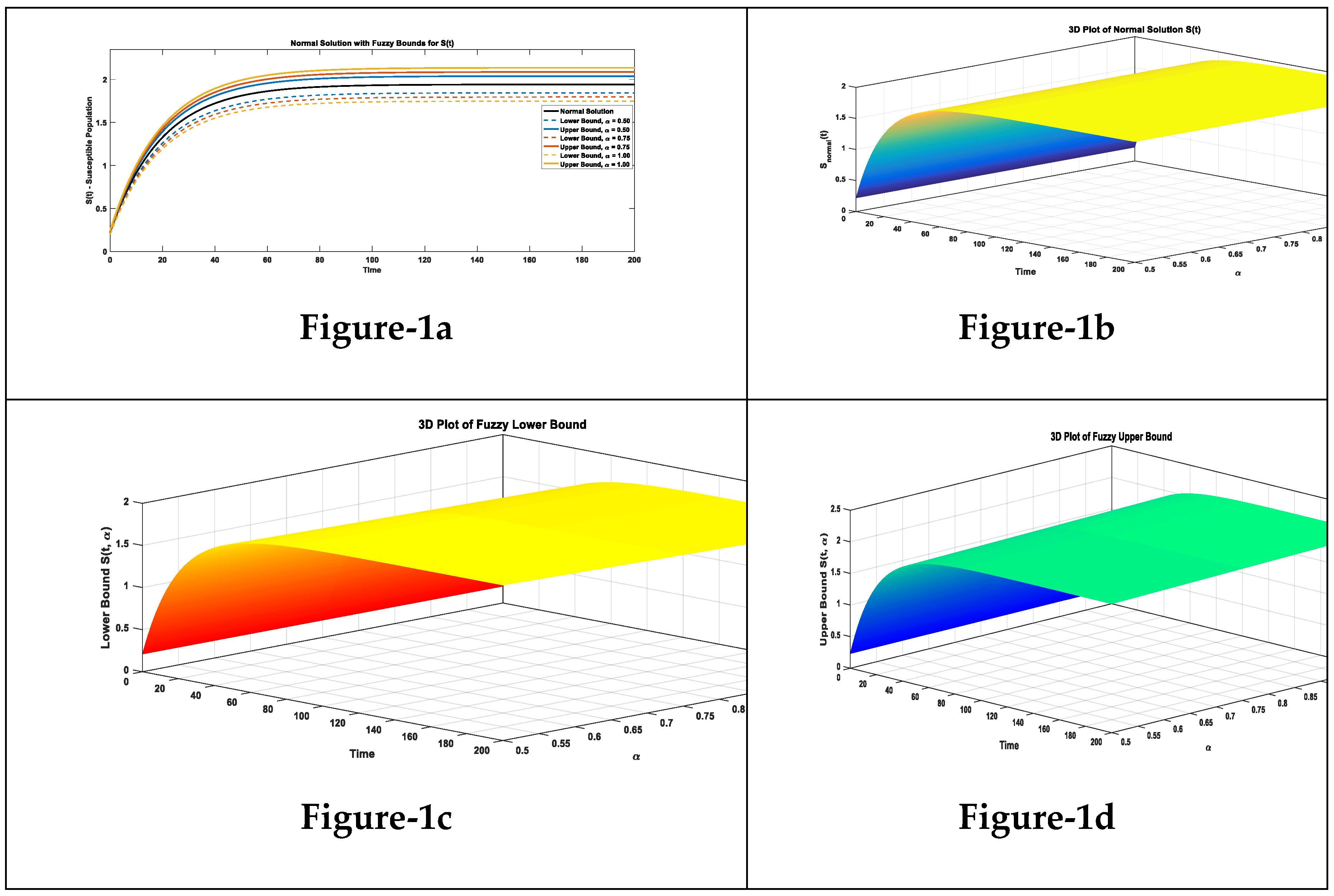
Figure 1. Graphical Representation of Susceptible Cases of Normal, Lower, Upper solution various values of α.

Figure 1. Graphical Representation of Susceptible Cases of Normal, Lower, Upper solution various values of α.

Comparison of approximate normal solution, fuzzy lower and upper bound solution for susceptible compartment for three terms at the given uncertainty values α ∈ [0, 1] against various fractional order

Table 3. Numerical Representation of Susceptible Cases of Normal, Lower, Upper solution various values of α.

Time (t)	[Normal,Lower, Upper] α = 0.50 Solution	[Normal,Lower, Upper] α = 0.75 Solution	[Normal,Lower, Upper] α =1 Solution
0	[0.2200 ,0.2090, 0.2310]	[0.2200,0.2035, 0.2365]	[0.2200,0.1980, 0.2420]
50	[1.8106,1.7200,1.9011]	[1.8106, 1.6748, 1.9464]	[1.8106,1.6295,1.9916]
100	[1.9318, 1.8352, 2.0284]	[1.9318 ,1.7869, 2.0766]	[1.9318,1.7386, 2.1249]
150	[1.9318 ,1.8352, 2.0284]	[1.9318,1.7869,2.0766]	[1.9318, 1.7386,2.1249]
200	[1.9318,1.8352, 2.0284]	[1.9318,1.7869, 2.0766]	[1.9318,1.7386, 2.1249]

Table 3. Numerical Representation of Susceptible Cases of Normal, Lower, Upper solution various values of α.

Time (t)	[Normal,Lower, Upper] α = 0.50 Solution	[Normal,Lower, Upper] α = 0.75 Solution	[Normal,Lower, Upper] α =1 Solution
0	[0.2200 ,0.2090, 0.2310]	[0.2200,0.2035, 0.2365]	[0.2200,0.1980, 0.2420]
50	[1.8106,1.7200,1.9011]	[1.8106, 1.6748, 1.9464]	[1.8106,1.6295,1.9916]
100	[1.9318, 1.8352, 2.0284]	[1.9318 ,1.7869, 2.0766]	[1.9318,1.7386, 2.1249]
150	[1.9318 ,1.8352, 2.0284]	[1.9318,1.7869,2.0766]	[1.9318, 1.7386,2.1249]
200	[1.9318,1.8352, 2.0284]	[1.9318,1.7869, 2.0766]	[1.9318,1.7386, 2.1249]

The susceptible compartment stabilizes near 1.93, while increasing α widens the fuzzy bounds. This shows that the system is sTable, but uncertainty grows with fuzziness, providing a realistic measure of variability.

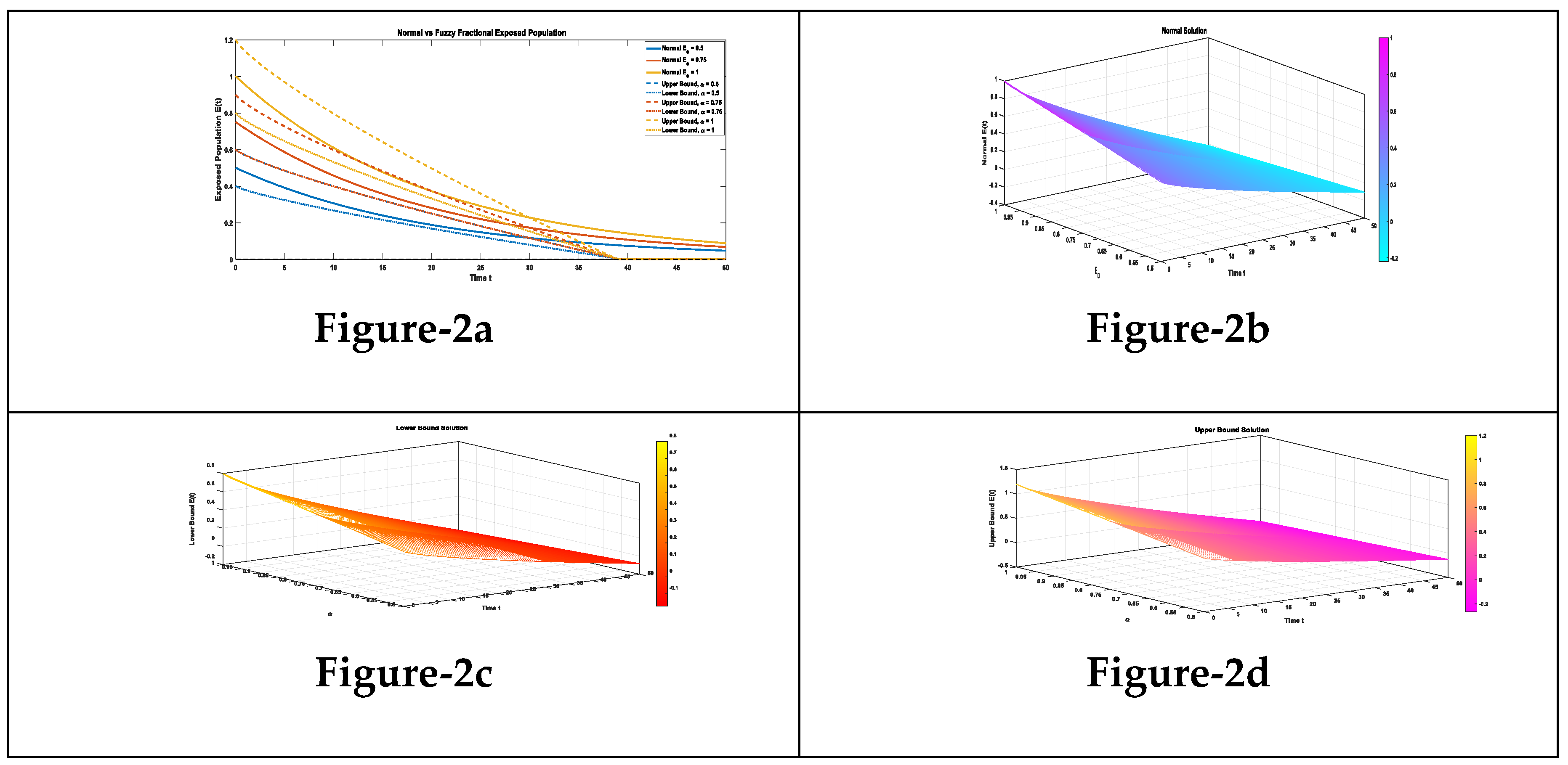
Figure 2. Graphical Representation of Exposed Cases of Normal, Lower, Upper solution various values of α.

Figure 2. Graphical Representation of Exposed Cases of Normal, Lower, Upper solution various values of α.

Comparison of approximate normal solution, fuzzy lower and upper bound solution for exposed compartment for three terms at the given uncertainty values α ∈ [0, 1] against various fractional order

Table 4. Numerical Representation of Exposed Cases of Normal, Lower, Upper solution various values of α.

Time (t)	[Normal,Lower, Upper] α = 0.50 Solution	[Normal,Lower,Upper] α = 0.75 Solution	[Normal,Lower, Upper] α =1 Solution
10	[0.3315, 0.2657, 0.3974]	[0.4962, 0.3974, 0.5949]	[0.6608, 0.5291, 0.7925]
20	[0.2067, 0.1661, 0.2472]	[0.3080, 0.2472, 0.3689]	[0.4094, 0.3283, 0.4905]
30	[0.0997, 0.0808, 0.1186]	[0.1469, 0.1186, 0.1752]	[0.1940, 0.1563, 0.2318]

Table 4. Numerical Representation of Exposed Cases of Normal, Lower, Upper solution various values of α.

Time (t)	[Normal,Lower, Upper] α = 0.50 Solution	[Normal,Lower,Upper] α = 0.75 Solution	[Normal,Lower, Upper] α =1 Solution
10	[0.3315, 0.2657, 0.3974]	[0.4962, 0.3974, 0.5949]	[0.6608, 0.5291, 0.7925]
20	[0.2067, 0.1661, 0.2472]	[0.3080, 0.2472, 0.3689]	[0.4094, 0.3283, 0.4905]
30	[0.0997, 0.0808, 0.1186]	[0.1469, 0.1186, 0.1752]	[0.1940, 0.1563, 0.2318]

The exposed population decreases rapidly with time across all α-values, approaching near zero by t = 30. The fuzzy bounds widen as α increases, reflecting higher uncertainty in the early phase of exposure. Importantly, the normal solution consistently lies between the lower and upper bounds, showing that the fuzzy framework successfully captures uncertainty while maintaining stability of the exposed dynamics.

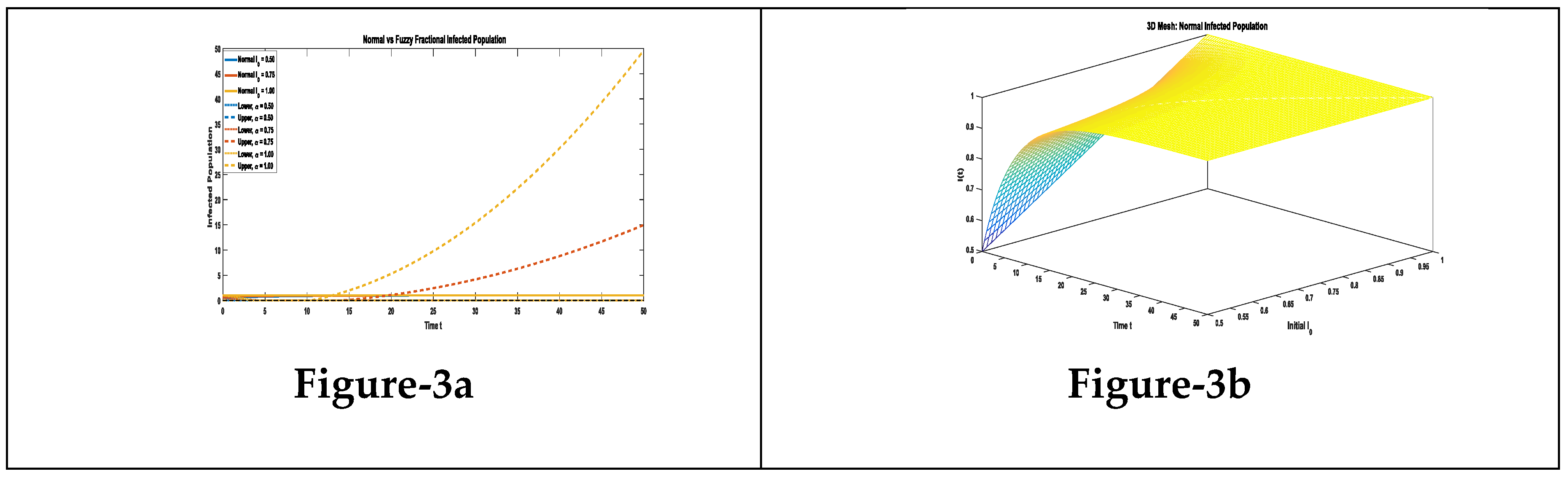
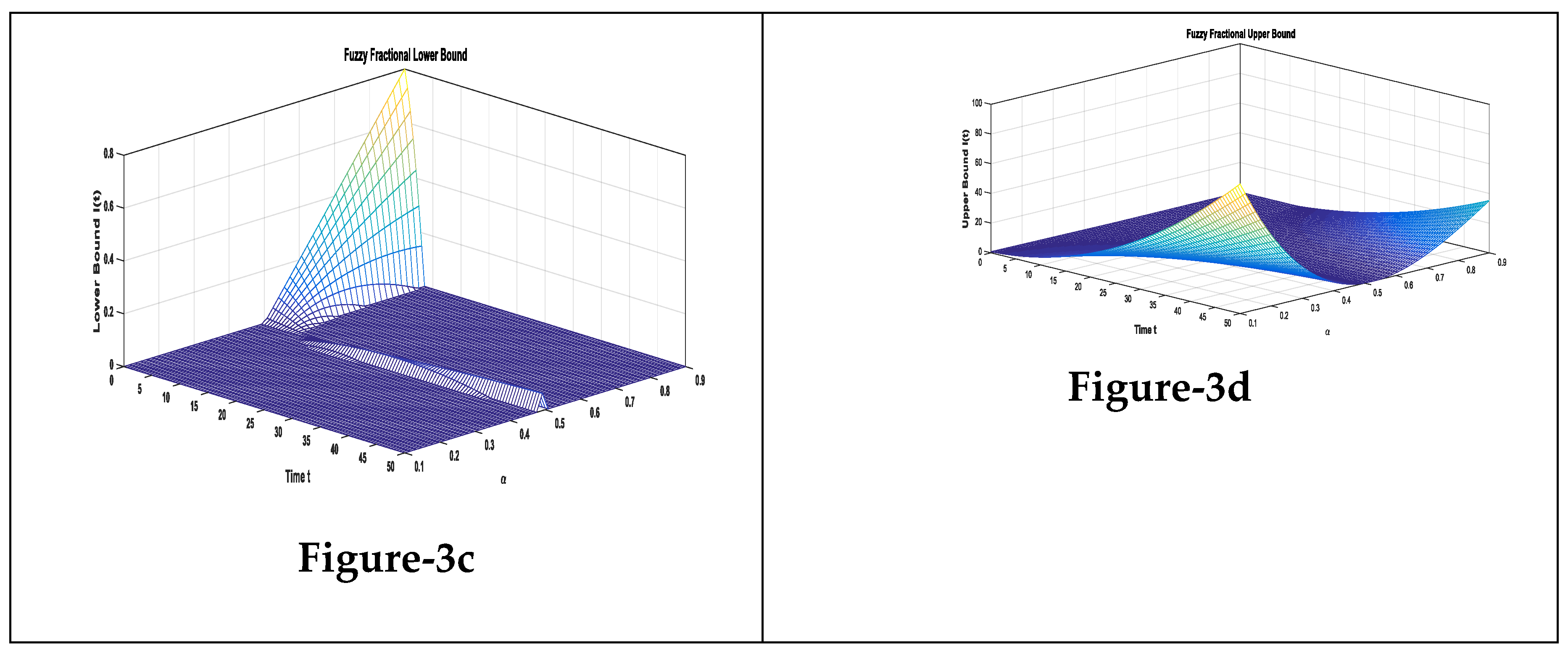
Figure 3. Graphical Representation of Infected Cases of Normal, Lower, Upper solution various values of α.

Figure 3. Graphical Representation of Infected Cases of Normal, Lower, Upper solution various values of α.

Comparison of approximate normal solution, fuzzy lower and upper bound solution for infected compartment for three terms at the given uncertainty values α ∈ [0, 1] against various fractional order

Table 5. Numerical Representation of Infected Cases of Normal, Lower, Upper solution various values of α.

Time (t)	[Normal,Lower, Upper] α = 0.50 Solution	[Normal,Lower, Upper] α = 0.75 Solution	[Normal,Lower, Upper] α =1 Solution
10	[0.3315, 0.2657, 0.3974]	[0.4962, 0.3974, 0.5949]	[0.6608, 0.5291, 0.7925]
20	[0.2067, 0.1661, 0.2472]	[0.3080, 0.2472, 0.3689]	[0.4094, 0.3283, 0.4905]
30	[0.0997, 0.0808, 0.1186]	[0.1469, 0.1186, 0.1752]	[0.1940, 0.1563, 0.2318]

Table 5. Numerical Representation of Infected Cases of Normal, Lower, Upper solution various values of α.

Time (t)	[Normal,Lower, Upper] α = 0.50 Solution	[Normal,Lower, Upper] α = 0.75 Solution	[Normal,Lower, Upper] α =1 Solution
10	[0.3315, 0.2657, 0.3974]	[0.4962, 0.3974, 0.5949]	[0.6608, 0.5291, 0.7925]
20	[0.2067, 0.1661, 0.2472]	[0.3080, 0.2472, 0.3689]	[0.4094, 0.3283, 0.4905]
30	[0.0997, 0.0808, 0.1186]	[0.1469, 0.1186, 0.1752]	[0.1940, 0.1563, 0.2318]

The infected population initially shows moderate values but rapidly declines over time across all α-levels, indicating the natural decay of infection spread in the model. At α = 0.50, the fuzzy bounds are the tightest and closely follow the normal solution,reflecting minimal uncertainty. With increasing α-values (0.75 and 1.00), the fuzzy bounds widen, capturing greater uncertainty in infection dynamics, though the lower and upper bounds still remain symmetrically close to the normal curve. Overall, the results suggest that while the infection diminishes consistently with time, the degree of uncertainty in the predicted infected population grows with higher fuzziness (α), highlighting the sensitivity of infection spread to uncertain parameters.

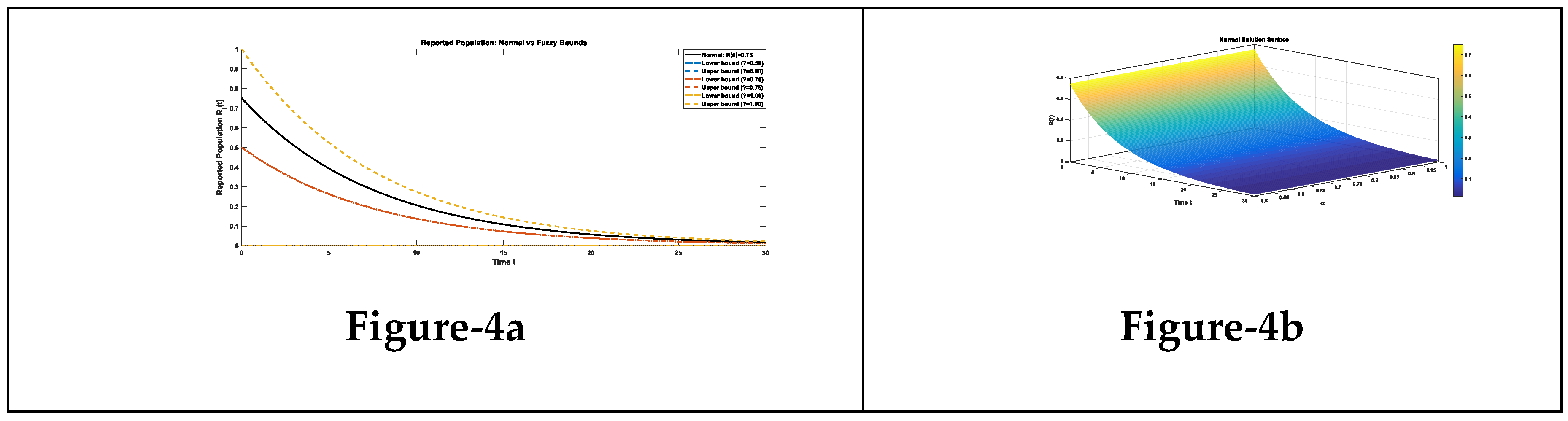
Figure 4. Graphical representation of reported Cases of Normal, Lower, Upper solution various values of α.

Figure 4. Graphical representation of reported Cases of Normal, Lower, Upper solution various values of α.

Comparison of approximate normal solution, fuzzy lower and upper bound solution for reported compartment for three terms at the given uncertainty values α ∈ [0, 1] against various fractional order

Table 6. Numerical representation of reported Cases of Normal, Lower, Upper solution various values of α.

Time (t)	[Normal,Lower, Upper] α = 0.50 Solution	[Normal,Lower, Upper] α = 0.75 Solution	[Normal,Lower, Upper] α =1 Solution
10	[0.2066, 0.0008, 0.2752]	[0.2066, 0.1380, 0.1380]	[0.2066, 0.0008, 0.2752]
20	[0.0564, 0.0011, 0.0749]	[0.0564, 0.0380, 0.0380]]	[0.0564, 0.0011, 0.0749]
30	[0.0163, 0.0011, 0.0214]	[0.0163, 0.0113, 0.0113]	[0.0163, 0.0011, 0.0214]

Table 6. Numerical representation of reported Cases of Normal, Lower, Upper solution various values of α.

Time (t)	[Normal,Lower, Upper] α = 0.50 Solution	[Normal,Lower, Upper] α = 0.75 Solution	[Normal,Lower, Upper] α =1 Solution
10	[0.2066, 0.0008, 0.2752]	[0.2066, 0.1380, 0.1380]	[0.2066, 0.0008, 0.2752]
20	[0.0564, 0.0011, 0.0749]	[0.0564, 0.0380, 0.0380]]	[0.0564, 0.0011, 0.0749]
30	[0.0163, 0.0011, 0.0214]	[0.0163, 0.0113, 0.0113]	[0.0163, 0.0011, 0.0214]

The reported population shows a rapid decline over time across all α-levels, with values becoming very small by t=30. At α = 0.50 and α = 1., the fuzzy lower and upper bounds remain close to the normal solution, indicating relatively small uncertainty in the prediction. In contrast, at α = 0.75, the bounds narrow significantly, suggesting more stability in the reported cases under this fuzziness level. Overall, the results imply that the reported population diminishes quickly over time, and the fuzzy framework confirms that the uncertainty in reported cases is minimal, with bounds consistently close to the normal trajectory.

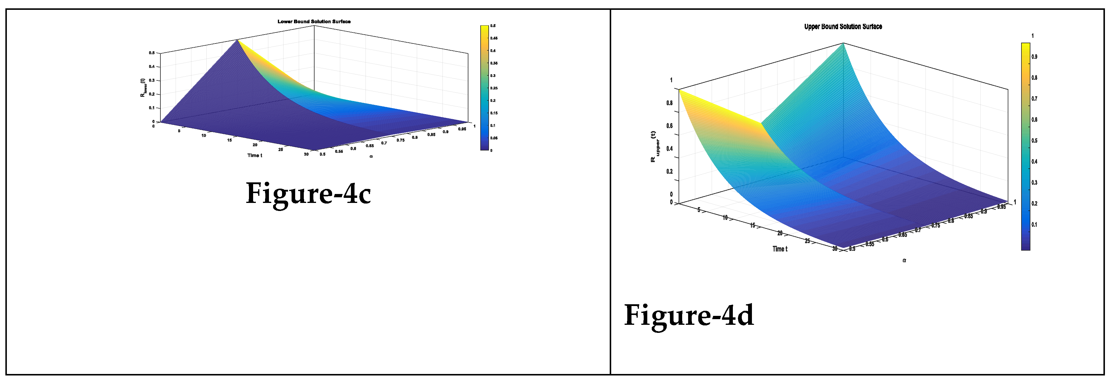
Figure 5. Graphical Representation of Unreported Cases of Normal, Lower, Upper solution various values of α.

Figure 5. Graphical Representation of Unreported Cases of Normal, Lower, Upper solution various values of α.

Comparison of approximate normal solution, fuzzy lower and upper bound solution for unreported compartment for three terms at the given uncertainty values α ∈ [0, 1] against various fractional order

Table 7. Numerical Representation of Unreported Cases of Normal, Lower, Upper solution various values of α.

Time (t)	[Normal,Lower, Upper] α = 0.50 Solution	[Normal,Lower,Upper] α = 0.75 Solution	[Normal,Lower, Upper] α =1 Solution
10	[0.2066, 0.0008, 0.2752]	[0.2066, 0.1380, 0.1380]	[0.2066, 0.0008, 0.2752]
20	[0.0564, 0.0011, 0.0749]	[0.0564, 0.0380, 0.0380]	[0.0564, 0.0011, 0.0749]
30	[0.0163, 0.0011, 0.0214]	[0.0163, 0.0113, 0.0113]	[0.0163, 0.0011, 0.0214]

Table 7. Numerical Representation of Unreported Cases of Normal, Lower, Upper solution various values of α.

Time (t)	[Normal,Lower, Upper] α = 0.50 Solution	[Normal,Lower,Upper] α = 0.75 Solution	[Normal,Lower, Upper] α =1 Solution
10	[0.2066, 0.0008, 0.2752]	[0.2066, 0.1380, 0.1380]	[0.2066, 0.0008, 0.2752]
20	[0.0564, 0.0011, 0.0749]	[0.0564, 0.0380, 0.0380]	[0.0564, 0.0011, 0.0749]
30	[0.0163, 0.0011, 0.0214]	[0.0163, 0.0113, 0.0113]	[0.0163, 0.0011, 0.0214]

The unreported population decreases sharply over time across all α-levels, with values approaching near zero by t=30t = 30t=30. The fuzzy lower and upper bounds remain closely aligned with the normal solution, indicating minimal uncertainty and confirming that unreported cases diminish rapidly under all considered scenarios.

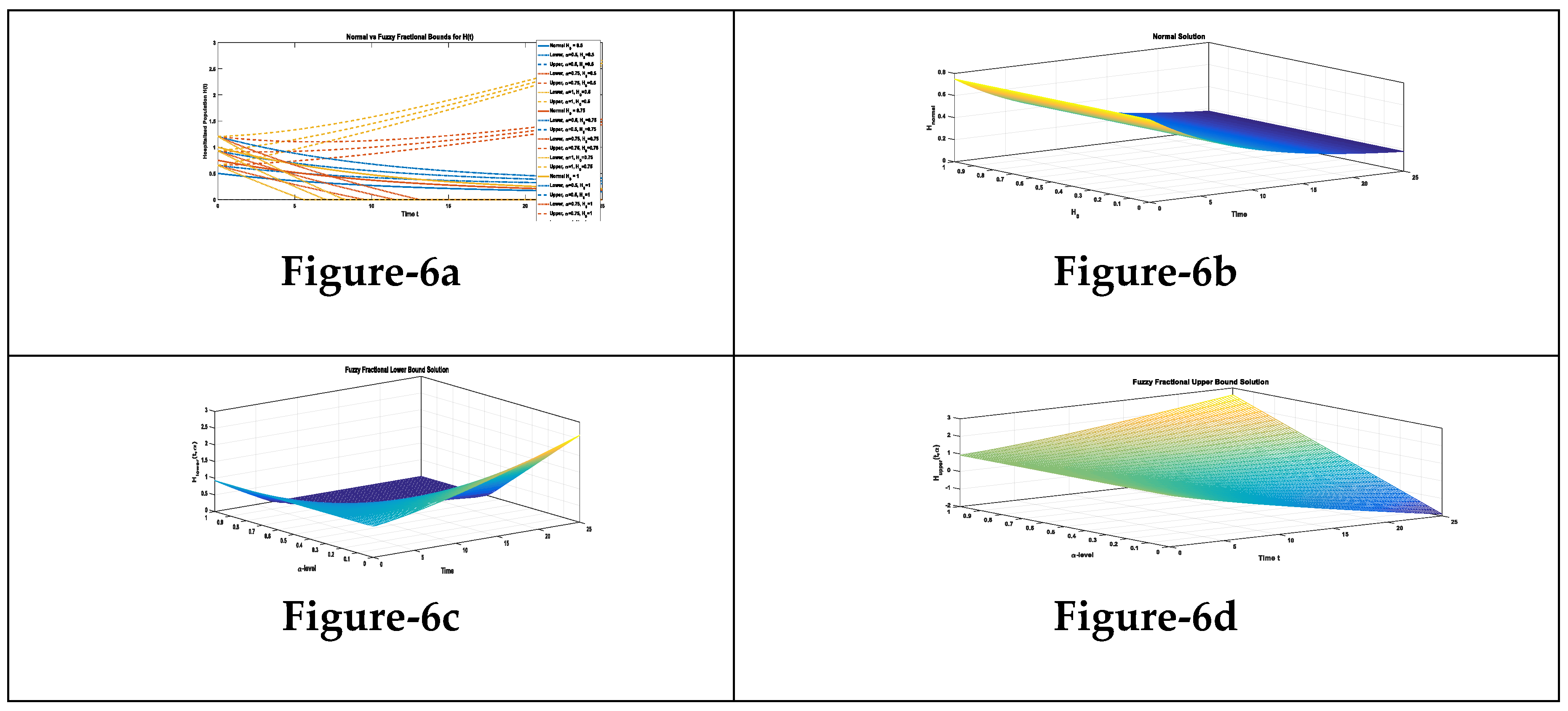
Figure 6. Graphical Representation of hospitalized Cases of Normal, Lower, Upper solution various values of α.

Figure 6. Graphical Representation of hospitalized Cases of Normal, Lower, Upper solution various values of α.

Comparison of approximate normal solution, fuzzy lower and upper bound solution for hospita compartment for three terms at the given uncertainty values α ∈ [0, 1] against various fractional order

Table 8. Numerical Representation of hospitalized Cases of Normal, Lower, Upper solution various values of α.

Time (t)	[Normal,Lower, Upper] α = 0.50 Solution	[Normal,Lower,Upper] α = 0.75 Solution	[Normal,Lower, Upper] α =1 Solution
10	[0.3686, 0.5157, 0.5784]	[0.3686, 0.0768, 1.0172]	[0.3686, 0.0000, 1.4561]
20	[0.2172, 0.3337, 0.4576,]	[0.2172, 0.0000, 1.3243]	[0.2172, 0.0000, 2.1911]

Table 8. Numerical Representation of hospitalized Cases of Normal, Lower, Upper solution various values of α.

Time (t)	[Normal,Lower, Upper] α = 0.50 Solution	[Normal,Lower,Upper] α = 0.75 Solution	[Normal,Lower, Upper] α =1 Solution
10	[0.3686, 0.5157, 0.5784]	[0.3686, 0.0768, 1.0172]	[0.3686, 0.0000, 1.4561]
20	[0.2172, 0.3337, 0.4576,]	[0.2172, 0.0000, 1.3243]	[0.2172, 0.0000, 2.1911]

The hospitalized population declines with time across all α-levels, but unlike other compartments, the fuzzy bounds show a much wider spread, especially at higher α-values. This indicates greater uncertainty in hospitalization dynamics, with the normal solution lying consistently between the lower and upper bounds. Overall, the results suggest that hospitalization is highly sensitive to parameter uncertainty, highlighting the variability in predicted outcomes under fuzziness

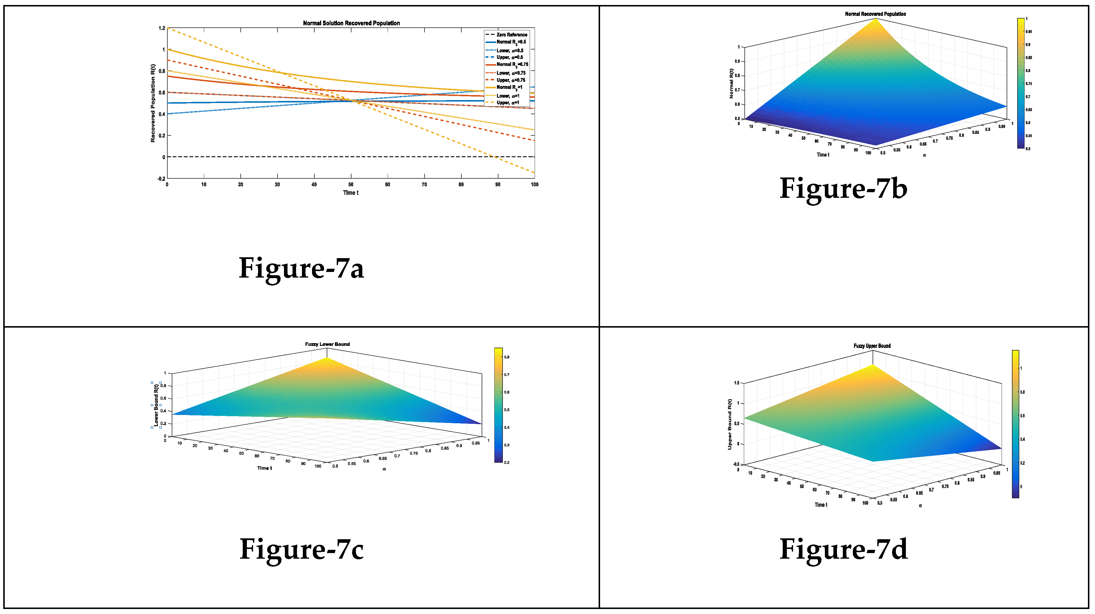
Figure 7. Graphical Representation of recover Cases of Normal, Lower, Upper solution various values of α.

Figure 7. Graphical Representation of recover Cases of Normal, Lower, Upper solution various values of α.

Comparison of approximate normal solution, fuzzy lower and upper bound solution for Recover compartment for three terms at the given uncertainty values α ∈ [0, 1] against various fractional order

Table 9. Numerical Representation of recover Cases of Normal, Lower, Upper solution various values of α.

Time (t)	[Normal,Lower, Upper] α = 0.50 Solution	[Normal,Lower,Upper] α = 0.75 Solution	[Normal,Lower, Upper] α =1 Solution
10	[0.5045, 0.4251, 0.5850]]	[0.7091, 0.5850, 0.8248]	[0.9137, 0.7449, 1.0647]
20	[0.5083, 0.4501, 0.5699]	[0.6757, 0.5699, 0.7497]	[0.8432, 0.6898, 0.9295]
30	[0.5113, 0.4752, 0.5549]	[0.6483, 0.5549, 0.6745]	[0.7854, 0.6347, 0.7942]

Table 9. Numerical Representation of recover Cases of Normal, Lower, Upper solution various values of α.

Time (t)	[Normal,Lower, Upper] α = 0.50 Solution	[Normal,Lower,Upper] α = 0.75 Solution	[Normal,Lower, Upper] α =1 Solution
10	[0.5045, 0.4251, 0.5850]]	[0.7091, 0.5850, 0.8248]	[0.9137, 0.7449, 1.0647]
20	[0.5083, 0.4501, 0.5699]	[0.6757, 0.5699, 0.7497]	[0.8432, 0.6898, 0.9295]
30	[0.5113, 0.4752, 0.5549]	[0.6483, 0.5549, 0.6745]	[0.7854, 0.6347, 0.7942]

The hospitalized population remains relatively table over time, with the normal solution consistently positioned between the fuzzy lower and upper bounds. The spread between bounds narrows as time progresses, indicating reduced uncertainty. Overall, hospitalization dynamics show moderate sensitivity to parameter fuzziness but maintain a steady trend across all α-levels.

8) 

Conclusions:

In this study, we have affirmed the existence and singleness of the solution to the fuzzy fractional-order model delineating COVID-19 infection. Additionally, we have outlined a systematic procedure for conducting the fuzzy Laplace transform paired with the Adomian decomposition method, facilitating an approximate solution to the envisaged model. Comparative analyses between fuzzy and conventional outcomes up to three terms have been presented, illustrating the efficacy of this method. Our observations reveal that the fusion of initial conditions as fuzziness with the fractional calculus approach remarkably elucidated the global dynamics of issues characterized by data uncertainty.