
Submitted:
14 September 2025
Posted:
16 September 2025
You are already at the latest version
Abstract
Alentejo and Algarve, regions of Southern Portugal, are characterized by a typical Mediterranean climate were evaporation plays a significant role in reservoir water budgets. Therefore, estimating water surface evaporation is essential for efficient reservoir water management. This study aims to (i) Assess the reservoir evaporation pattern in Southern Portugal, from meteorological offshore measures; (ii) benchmark various indirect methods for evaluating reservoir evaporation at a monthly scale and (iii) provide recommendations on the most suitable indirect method to apply in operational practices.
Keywords:
Mediterranean region
; reservoirs
; offshore measurements
; evaporation
; benchmarking analysis
1. Introduction
The Mediterranean climate is characterized by its accentuated inter-annual variability and is one of the world’s hot spots of climate change. At the end of this century, climate models project an increase in air temperature (ranging between 2.2 and 5.1 °C), a decrease in rainfall (ranging between 4% and 27%), and an increase in drought periods [1]. Consequently, climate change impacts on the Mediterranean region will particularly affect the availability of water resources.
In the regions of Alentejo and Algarve in Southern Portugal, where a Mediterranean climate prevails, the availability of water relies on man-made infrastructures, such as dams and reservoirs, which are strategic elements for securing urban and industrial water supply, irrigation, and energy generation due to the challenges presented by water scarcity in this region [2,3,4,5]. However, the construction of reservoirs alters the water balance of the region and increases the loss of water resources to the atmosphere through evaporation.
Evaporation from an open water body, also known as lake evaporation and referred to as reservoir evaporation throughout this paper, is one of the most important components of the water balance. According to statistics, the annual evaporation losses of the reservoirs in arid and semi–arid regions account for about 40% of the total usage volume [6].
In Southern Portugal region, most reservoir managers use 1000 mm as the reservoir’s annual evaporation for simplification in water balance. Others, estimate evaporation based on the mean reference evapotranspiration for the evolving reservoir region [7]. The lack of rigour in both approaches highlights the need for better estimation of evaporation in reservoirs.
The evaporative losses from reservoirs can be calculated by subtracting the natural evapotranspiration that would have occurred on the land from the evaporation caused by the flooded surface [8]. Alternatively, studies estimating evaporation can use aerodynamic mass transfer formulations, energy balance formulations, or a combination of both. The energy source for the evaporative process can be solar radiation, atmospheric radiation, the sensible heat of the overlying air layer, or energy stored in the water body. Various methods have been developed for quantifying evaporation in reservoirs. These methods can be classified according to theoretical developments, as discussed by [9]: (1) water balance applied to the water body, (2) energy balance applied to the water body in the reservoir, (3) aerodynamic functions (mass transfer), (4) hybrid with energy balance and aerodynamic, (5) thermic as function of the temperature, and (6) direct measurements.
A significant limitation of most of these methods is that they require site-specific measurements of several meteorological variables, such as air/water temperature, humidity, wind speed, and solar radiation, that are not commonly available at the reservoir’s water surface. To overcome such limitations, this study was based on data collected from floating weather stations on instrumented platforms across 9 reservoirs in Alentejo and Algarve for the period 2002-2006. The complementary water temperature profile measurements at the floating platforms enabled the method of energy balance to be considered as a reference benchmark for comparison with other methods due to its accuracy [10,11,12].
This study aims to identify the most appropriate model for assessing evaporative losses from reservoirs and to provide recommendations for use in operational practices in Mediterranean climate regions.
2. Materials and Methods
2.1. Study Area
Alentejo and Algarve, located in southern Portugal (Figure 1), have a Mediterranean climate of type Csa, according to the Köppen classification. This corresponds to a temperate climate with hot, dry summers (IPMA, https://www.ipma.pt/en/oclima/normais. clima/, last access: 21 Mar 2025), and this type of climate can be found throughout the Mediterranean basin [1] and some regions of Australia and California (USA).
Based on the climatological normal of 1981-2010 (Instituto Português do Mar e da Atmosfera, IPMA, https://www.ipma.pt/en/oclima/ normais.clima/1981-2010/ normalclimate8110.jsp, last access: 21 Mar 2025) the warmest months in southern Portugal are July and August, with average temperatures ranging between 23.0 °C in Setúbal and 24.8 °C in Beja. In Faro and Beja, the average maximum temperatures can reach 28.8 °C and 33.3 °C, respectively, while on extreme days, temperatures can exceed 45 °C in the interior of Alentejo. The coldest months are January and February, with average temperatures ranging between 8.6 °C in Portalegre and 12.0 °C in Faro. During these months, average minimum temperatures vary between 4.9 °C in Setúbal and 7.9 °C in Faro, and negative temperatures may occur, especially in regions far away from the coastline. The average annual total rainfall varies between 511.6 mm in Faro and 833.1 mm in Portalegre, with the rainiest months being November and December, with monthly values of 91.9 mm in Évora and 128.3 mm in Portalegre.
Nine reservoirs were selected across the region (Figure 1) and the main morphometric characteristics are presented in Table 1. Reservoirs are mainly used for irrigation and domestic water supply, resulting in significant fluctuations in water levels during the dry season as large volumes of water are mobilized to meet these needs.
2.2. Floating Stations
A floating monitoring stations was designed and built for each one of the selected reservoirs, to record meteorological and water temperature data. These stations are part of the Portuguese Water Resources Monitoring Network (SNIRH, https://snirh. apambiente.pt, last access: 21 Mar 2025) and were installed over wooden floating platforms with a 30 m2 area, anchored in place by ropes tied to three sunk concrete blocks. The meteorological station installed on each platform records pan evaporation, downward solar radiation, atmospheric pressure, precipitation, air temperature, air relative humidity, and wind speed and direction. Data are recorded at a frequency of one value per 10 minutes, except precipitation and wind speed, which are recorded every minute according to precipitation events. Data are used on an hourly average scale. To reduce the effects of direct solar radiation on the walls of the pan and ensure closer proximity between the temperatures of the water in the pan and in the reservoir, the pan is recessed into the platform, contacting the reservoir water. Wind speed and direction, air temperature, and relative humidity are recorded at three levels (2, 5, and 8 meters), and the vertical wind speed sensor is located 2 meters above the water surface on an additional rod that includes a sensor for measuring atmospheric pressure and solar panels for charging the system batteries. The water temperature in the reservoirs was also monitored continuously using five sensors placed at depths of 1, 5, 10, 15, and 20 meters. These sensors were installed along a steel cable with a ballast at its lower end to keep the cable in a vertical position. To protect the probes and reduce the risk of any winding in the mooring cables of the platform, the entire assembly, including the cable and sensors, is positioned inside a perforated tube (high-density polyethylene) with a 90 mm diameter. A schematic layout and dimensions of the floating monitoring stations are presented in Figure 2.
The floating stations were installed in 2001 with the exception of Alqueva reservoir where the station was established in 2002. All measurements were parametrized, pre-processed, and temporarily stored in a data acquisition system, GEOLOG S (Logtronic, GmbH), expanded in its standard configuration to accommodate all sensors. The locally stored data was transmitted via GSM to the SNIRH central repository, either daily or upon request.
2.3. Meteorological Data and Water Body Temperature
Meteorological and water body temperature data from the 9 floating stations were recorded between 2002 and 2006 by the first author.
The annual cycle and daily data of air temperature, air relative humidity, wind speed, and solar radiation at 2 meters high were characterized. Water surface temperature was also analysed. The graphical representation of the data time series is presented at Figure 3.
The annual cycle of air temperature between the different reservoir locations shows great homogeneity, ranging from 8.5 to 24.2 °C. During winter, the highest temperatures are observed in reservoirs located further south, particularly in Bravura, which records temperatures about 4 °C higher than those in other reservoirs. During summer, Odeleite has higher air temperatures, while Bravura has lower air temperatures. It can be verified that the air temperature in the Bravura reservoir has the lowest amplitude and the smallest variation throughout the year, which can be attributed to its proximity to the sea. The behaviour of air relative humidity is identical to that of air temperature. The recorded values fall within the expected range for the region, with the highest values (> 80 %) occurring in November, December, and January, and the lowest values (< 50%) occurring in the summer months. The lowest value was recorded in July, during which the variability between reservoirs was more pronounced. The Bravura reservoir exhibited the lowest amplitude, ranging from 65.7% in July to 80.3% in November. Significant differences in wind speed were observed between reservoirs. While the annual cycle in each reservoir demonstrated a smooth variation, a slight upward trend in wind speed during summer months was noted, particularly in Bravura and Odeleite reservoirs. This increase in wind speed may be attributed to the summer breeze characteristic of southern Portugal afternoons and may explain the greater variability in wind speed values observed in these two reservoirs, whose local physiography favours the establishment of long fetches from the north quadrant. Maranhão and Pego do Altar reservoirs consistently exhibited the lowest wind intensity throughout the year. The behaviour of incoming solar radiation is quite similar across all nine reservoirs. The annual cycle of solar radiation is consistent for most of the reservoirs, with identical behaviour in winter across all reservoirs. However, during summer months, higher values are observed in Santa Clara and Bravura reservoirs, while lower values are observed in Maranhão reservoir.
Figure 4 presents daily water temperatures () recorded at depths of 1, 5, 10, 15, and 20 meters in the reservoirs. Spatial and temporal analysis of water temperature reveals consistent thermal behaviour between reservoirs, with the greatest amplitudes occurring at the surface, ranging between 16-18 °C. The highest water surface temperatures range between 25-27 °C and are observed in July and August. At the maximum monitored depth (20 m), recorded water temperature amplitudes varied between 8-10 °C. Minimum values were observed in January and February, with most reservoirs recording values not falling below 10 °C.
The temperature profiles exhibit a consistent annual cycle across most reservoirs. In January, all reservoirs display an isothermal profile. As air temperature, solar radiation, and day length increase in April, the water column experiences deep heating, leading to thermal stratification that reaches its peak during summer. By June, some reservoirs exhibit an upper-mixed layer, characterized by constant temperature (upper-mixed layer induced by surface agitation) overlapping a layer where the temperature varies with depth (thermocline). As autumn begins, the surface temperature gradually decreases, extending to deeper layers and leading to a progressive reduction in the thermocline until the isothermal profile is re-established in January or February.
2.4. Reservoir Evaporation Process
The conservation energy law accounts for incoming and outgoing energy, balanced by the amount of energy stored in the system.
The energy balance herein considered can be expressed as:
where is the net radiation, is the heat storage change in the water body, H is the sensible heat flux, is the latent heat flux, is the net heat flux carried by surface water and groundwater and, is the net heat flux resulting from precipitation. All fluxes are in units of W m−2.
The last two terms of Eq.1 have been neglected because of their relatively small magnitudes compared to the other terms in the balance [13,14,15]. Consequently, the energy balance equation can be simplified:
The reservoir evaporation was calculated considering that the flux of sensible heat (H) is related to the latent heat flux () through the Bowen ratio () [16,17]. Although some limitations have been identified in previous research [11,18,19,20], the Bowen Ratio Energy Budget (BREB) method was selected as the reference, as it’s recognized as a standard by which other methods are compared [10,11,12,21].
In the absence of on-site atmospheric radiation () measurements, the European Centre for Medium-Range Weather Forecasts (ECMWF) analysis was used (http://www.ecmwf. int/products/forecasts/d/charts, last access: 21 Mar 2025).
The energy balance closure (EBC) was calculated by:
2.5. Indirect Methods to Calculate Evaporation
Estimating evaporation from a large open water surface is a challenging task, with many different methods available. These methods can be broadly categorized as mass transfer, combination of energy balance and mass transfer, temperature, and pan evaporation methods [11,22]. In this paper, five different evaporation methods were studied, and their mathematical formulations are detailed in Table 2. The BREB formulation is also presented.
The mass-transfer method (MT) is one of the oldest [24,32] and most widely used approach for estimating open water evaporation due to its simplicity and reasonable accuracy. The input variables are wind speed and the difference of vapour pressure between actual and saturated vapour pressure [33]. This method assumes that the evaporation rates are a linear function of the wind speed, the difference between the vapour pressure at the water surface and the atmosphere, and the empirical mass transfer coefficient, [18,23,34]. The mass transfer coefficient, N, is usually site-depend on various factors such as the lake shape, location and height of meteorological measurements, climatic conditions, and more [18]. An equation for N, as function of As, is presented for each of the studied reservoirs in section 3 of this paper. For other reservoirs, in Mediterranean climate regions, can be applied a general equation achieved and presented in section 3, too.
Penman [24,35] developed a combined approach of the mass transfer and energy budget methods that eliminated the need for water surface temperature in estimating open water evaporation. The Penman equation consists of two terms, commonly referred as the "energy term" and the "aerodynamic term". The first term represents the minimum possible evaporation rate, also known as the "equilibrium rate". The second term accounts for the influence of wind on evaporation through a wind function and the drying capacity of the atmosphere. The success of the Penman equation (PEN) in various locations is due to its solid physical foundation because it combines the mass transfer and the energy balance methods [36].
Priestley and Taylor [26] proposed a simpler version of Penman’s equation by considering evaporation as a function of the energy term only, as they believed the aerodynamic term could be approximated as a fixed fraction of the total evaporation. Suggesting that the aerodynamic term contributes 21% of the total evaporation, then an empirically derived parameter, , with an averaged value of 1.26, was introduced for the energy component [37]. The Priestley-Taylor equation (PT) does not require wind speed data or the determination of the wind function for its application. [27] formulated the PT method as a truncated version of the Penman equation, where the aerodynamic component was dropped, but a coefficient greater than 1.0 is included as a multiplier.
The Thornthwaite method (THOR) [28] is a widely used method for estimating monthly potential evapotranspiration. This method correlates mean monthly temperature with evapotranspiration, which is determined from water balance for valleys with sufficient moisture to maintain active transpiration [38]. [39] provide estimates of lake evaporation using the THOR formula and compare them with estimates from other models.
The most used evaporation method is the standard pan evaporation (PE) approach [31,40,41]. Pan evaporation (measured US class A pan evaporation) has been widely used to monitor reservoir evaporation operationally [7,42,43] and in lake modelling studies [44]. Commonly, a reduction coefficient is applied to minimize the "oasis effect" caused by the advective heat and account for the large quantities of energy received through the base and sides of the pan. In lake studies [36,45], a value of 0,7 for the annual pan coefficient is usually used. However, several authors [46,47] refer that pan coefficients vary throughout the year and should be calculated for each month individually. While many studies have identified the limitations of this approach [47,48,49,50], it remains widely used, as a source for large-scale validations due to its simplicity and moderate data requirements [43]. In this study, due to specific pan settlement on the floating platform, as previously referred in to section 2.2, the measured evaporation at the pan should be identical to real evaporation over the inundated area at the site. The factors that determine high pan evaporation rates usually observed on terrestrial frameworks are minimized here as the pan was placed offshore, on the floating platform, in contact with the water body surface.
2.6. Methods Performance Evaluators
3. Results and Discussion
3.1. Reservoirs Evaporation Estimation
Considering the energy balance, Table 5 shows the annual mean energy fluxes for the nine reservoirs, and the energy balance closure (EBC).
For most reservoirs, the heat storage change () is close to zero confirming that the net heat flux carried by surface water and groundwater () and the net heat flux resulting from precipitation () can be neglected. The shows good results for almost reservoirs, except for Bravura, Caia, and Maranhão. Comparing Bravura and Odeleite, despite Bravura being located under more Atlantic influence with a different wind pattern and a smaller surface area, the latent heat flux can be overestimated. For the Caia and Maranhão reservoirs, which are located at higher latitudes, the incoming atmospheric radiation may be underestimated when compared to Pego do Altar, which lies further inland at a much higher altitude. These findings allow us to conclude that even for these reservoir the net heat flux carried by surface water and groundwater () and the net heat flux resulting from precipitation () can be neglected.
The monthly values for the different components of the heat budget, including net radiation, latent heat, sensible heat, and heat storage change, are illustrated in Figure 5.
The monthly variation of latent heat flux () exhibits a strong seasonality, which aligns with the net radiation (), the primary energy source for the heat balance. The maximum flux typically lags the peak values of . On the other hand, the minimum flux is primarily influenced by the heat storage change (). In most reservoirs, the annual approaches zero, indicating a null balance between energy gains and losses throughout the years. The energy dynamics of the reservoirs can be understood by analysing the gains and losses of energy by the water body over the year. During spring, the reservoirs experience an energy gain and storage phase, driven by net radiation and low evaporation rates. Generally, the energy begins to increase from February or March until August, reaching its maximum around April (although this timing can vary across years and reservoirs, sometimes occurring in May or June). From September onwards, the energy storage variation reverses, and the water mass undergoes an energy reduction, typically lasting until January, with the maximum energy loss occurring in November. exhibits large positive and negative values, ranging from 55.2 to 88.8 W m−2 and −45.7 to −93.1 W m−2, respectively. During autumn, as solar radiation decreases, the energy required for evaporation is sourced from the release of in the form of and, to a lesser extent, H. fluxes display seasonal trends, with the highest values observed in summer, following a similar pattern to solar radiation (). However, in some winter months, negative values of can be observed. The annual mean ranges from 68 to 92 W m−2, for all reservoirs as shown in Table Figure 5. H depends on the temperature difference between the water surface () and the air (). H has relatively low values compared to other components of the energy balance. It is generally positive since, on average, is higher than . Under these conditions (), the sensible heat flow occurs from the water surface to the atmosphere, resulting in energy loss from the lake.
Daily evaporation values were determined for all reservoirs using the BREB method, as described by Eq. 4. The monthly evaporation is presented in Figure 6. To identify possible outliers the annual cycle of mean, maximum, and minimum evaporation were also presented. Although there are no substantial inter-annual variations in evaporation, a pronounced seasonality is evident. The highest evaporation rates are observed from June to August, while the lowest rates occur between December and February. Generally, the monthly mean evaporation falls within the expected range for each respective month, indicating a reasonable consistency throughout the period.
When comparing the monthly evaporation rates shown in Figure 7, it is evident that July has the highest evaporation values, while January experiences the lowest rates. The maximum monthly evaporation ranges from 4.4 mm d−1 in the Maranhão reservoir to 6.7 mm d−1 in the Bravura reservoir. In general, the minimum monthly evaporation is nearly zero for most reservoirs, except for Alqueva and Santa Clara, which have values ranging from 0.4 to 0.6 mm d−1, respectively. Across all reservoirs, the monthly evaporation varies from 0.8 mm d−1 in winter to 4.0 mm d−1 in summer, with an average of 2.7 mm d−1. These values align with other measurements in the Mediterranean region, as reported in studies by [52] or [53].
Figure 8 illustrates the spatial distribution of mean seasonal reservoir evaporation values in southern Portugal. The values were obtained through inverse distance interpolation for the dry and wet semesters, respectively. Figure 9 displays the spatial distribution of mean annual reservoir evaporation values. The patterns of reservoir evaporation exhibit distinct seasonal and spatial variations. Throughout the year, a clear minimum is observed in the northern part of the region, while the maximum values are concentrated in the south-west Algarve region. This spatial pattern is consistent in both the dry and wet semesters. The annual evaporation losses range from 750 to 1230 mm, showing a significant positive gradient from the northern part of the region towards the south-west Algarve region. This indicates that the reservoirs in the Algarve region experience higher evaporation rates compared to those in the northern areas.
3.2. Benchmarking of Indirect Methods
A monthly benchmarking analysis was performed to assess the performance of different indirect methods for estimating reservoir evaporation. Five different evaporation methods, as outlined in Table 2, were employed to calculate the reservoir evaporation for the 9 reservoirs under study.
Figure 10 illustrates the comparison between monthly evaporation estimates obtained from the 5 indirect methods and the evaporation estimated with the BREB method, using the Alqueva reservoir as an example. The figure displays the trend line and the 1:1 line (left) and the differences in average monthly evaporation for both the wet and dry semesters (right). Table 6 presented the same results for all reservoirs.
MT method
Table 7 presents the estimation of the mass transfer coefficient (N) for each reservoir. There is a strong correlation () between the evaporation rates estimated by the energy budget method and the mass transfer product . However, variations in N were observed among the reservoirs, which can be attributed to differences in exposure to prevailing winds and physiographic characteristics of the water bodies. It was observed that the mass transfer coefficient decreases with an increase in the water surface area of the reservoirs, which is consistent with the findings from studies conducted on lakes in the USA (Mirror, Hefner, Mead) [18] and the Greek lake Vegoritis [54]. The calculated N value for these lakes was slightly higher than the values obtained in our study, resulting in higher evaporation rate estimates for those cases. This discrepancy can be attributed to differences in measurement procedures, such as the measurement of atmospheric humidity being conducted on the shore upwind of those lakes, while in our study, all measurements were made offshore in the reservoir.
A overall relationship between N and the reservoir water surface area (), was established to be applied in Mediterranean climate region:
The comparison between monthly evaporation estimated using the MT method and the evaporation estimated using the BREB method is presented in Figure 10 and Table 6. The trend lines closely follow the 1:1 line, indicating a high level of accuracy in the MT method’s estimation of evaporation for all nine reservoirs. However, there is a slight underestimation observed for the largest studied reservoir (Alqueva), and some overestimation was observed for the smaller studied reservoir (Bravura). In addition to the differences in reservoir size, the higher wind speeds observed at the Bravura site, as discussed in section 3.1, may contribute to these discrepancies in evaporation estimates by the MT method. Regarding the average monthly, the differences were ± 1 mm d−1 for all reservoirs.
PEN method
The PEN method consistently overestimates annual evaporation, with the most pronounced positive bias occurring during dry season months. The best estimates of evaporation using the PEN method are obtained for reservoirs where the wind speed is consistently lower. This can be attributed to the reduced aerodynamic term in the Penman equation, which leads to smaller evaporation estimates and reduces the bias compared to the BREB values. Reservoirs such as Pego do Altar and Santa Clara exhibit nearly zero bias in evaporation estimates when using the PEN method.
PT method
Monthly average evaporation rates estimated by PT method and BREB show a good fit, and it can be observed that in eight out of nine reservoirs, there is a consistent underestimation of evaporation throughout the year. This finding is contrary to what is typically reported in the literature [11]. The standard coefficient () value of 1.26 used in the PT method takes into account the proportion of energy mobilized for evaporation through advection [55,56]. However, in our specific conditions, this coefficient seems to be insufficient. The observed underestimations of evaporation using the PT method indicate the need to increase the standard coefficient () value by 10%, suggesting that moderate advection occurs at the reservoir sites.
THOR method
The THOR method, based on the Thornthwaite formula using air temperature measurements only, showed surprisingly good agreement with the standard BREB method, considering its simplicity. However, the evaporation estimates tended to underestimate evaporation during the dry semester in most reservoirs, except for Maranhão and Pego do Altar, where the fit was good. The underestimation was more pronounced in Bravura and Santa Clara reservoirs, with average biases of −1.10 mm d−1 and −1.04 mm d−1, respectively.
PE method
In PE method, the trend lines closely align with the 1:1 line, indicating a strong positive correlation between pan measured evaporation and BREB estimated evaporation for eight reservoirs ( values greater than 0.95). However, in the Maranhão reservoir, the pan measured evaporation exceeded the estimated evaporation by 24%. When considering the average monthly difference, there is nearly zero annual bias in most reservoirs, except for Bravura and Maranhão reservoirs. In Bravura, the dry semester exhibits the highest negative bias (-1.38 mm d−1), while in Maranhão, the maximum bias is positive (0.59 mm d−1), also occurring in the dry semester.
Figure 11 shows the average and standard deviation of the monthly differences between BREB evaporation values and estimates obtained from the five alternative evaporation methods. All methods yield evaporation estimates identical to BREB values during the wet semester, regardless of the reservoir considered. In the dry semester, all methods provide small biases, but the standard deviations vary substantially depending on the reservoir. Larger standard deviations can be observed in the MT evaporation estimates for Bravura reservoir, and in the PEN values for Maranhão and Pego do Altar reservoirs.
3.3. Ranking of Evaporation Methods
The evaluation of evaporation methods is presented using the statistical descriptors in Table 3. Table 8 provides the statistics and performance of the methods for all reservoirs. The MT method exhibits the highest Root Mean Square Error (RMSE) value of 1.6 mm d−1 in Bravura reservoir, while the PEN method shows the lowest value of 0.16 mm d−1 in Pego do Altar reservoir. The range of RMSE varies from 0.25 to 0.44 mm d−1 for most reservoirs, except for Santa Clara and Bravura, which have values of 0.73 mm d−1 and 0.95 mm d−1, respectively.
The ranking of methods was determined based on the Index of Performance (d) (Table 8) and the Taylor diagram [57] (Figure 12).
The performance of the five methods was classified as Excellent for Alvito, Caia, Odeleite, Pego do Altar e Roxo reservoirs. The PEN and/or PT methods generally performed better, except for Caia reservoir where the PE method showed better performance (Table 8). These findings are consistent with the results from the Taylor diagram (Figure 12).
The Taylor diagram enables stakeholders to identify the better method to applies by considering the study objectives, data availability, and time scale. For instance, in the Alqueva reservoir, the PT, THOR, and PE methods provide an excellent representation of variability, although the PEN method shows a stronger correlation. In Pego do Altar, the PEN and PT methods achieve a correlation coefficient and an NSD equal to one, with an RMSE close to zero, indicating an almost perfect agreement with the observed data.
4. Conclusions
This study presents a set of offshore meteorological data namely: pan evaporation, downward solar radiation, atmospheric pressure, precipitation, air temperature, air relative humidity, wind speed, wind direction, and reservoir water temperature on different levels (1,5,10,15, and 20 meters), obtained in nine meteorological and water temperature floating stations built in nine reservoirs located in Southern Portugal. The nine reservoirs are: Alqueva, Alvito, Bravura, Caia, Maranhão, Odeleite, Pego do Altar, Roxo, and Santa Clara.
At annual scale, the simplified four-term energy balance model, accurately represented the evaporation process in the reservoirs. There are 3 exceptions: Bravura, Caia and Maranhão that must be carefully considered.
The monthly analysis of the heat budget revealed significant variations in the latent heat flux (), which closely aligned with the changes in net radiation (). The peak values of generally occurred shortly after the peak values, indicating a slight time lag. On the other hand, the minimum flux was predominantly influenced by the heat storage change () within the reservoir system. Most reservoirs exhibited an annual approaching zero indicating a null balance between energy gains and losses throughout the years. The sensible heat flux (H) showed relatively low values compared to other components of the energy balance. Results reveal a clear seasonal pattern, with July consistently exhibiting the highest evaporation values, while January experiences the lowest rates. Across all reservoirs, the monthly evaporation varies from 0.8 mm in winter to 4.0 mm in summer, with an average of 2.7 mm . Reservoir evaporation losses demonstrate noticeable seasonal and spatial variations. The northern part of the region consistently exhibits a minimum evaporation throughout the year, while the south-west Algarve region shows maximum values. This spatial pattern remains consistent during both the dry and wet seasons. The annual evaporation values span from 750 to 1230 mm, indicating a significant positive gradient from the northern part of the region towards the south-west Algarve. Consequently, it can be inferred that reservoirs in the Algarve region generally experience higher evaporation rates compared to those in the northern areas.
Water reservoir managers often do not have access to these data, for that reason a benchmarking analysis of indirect methods [Mass Transfer (MT), Penman (PEN), Priestley and Taylor (PT), Thornthwaite (THOR), and Pan Evaporation (PE)] was carried out. The performance of the methods were evaluated by d index and Taylor diagram. Concerning MT method, an equation for mass transfer coefficient (N) function of the reservoir water surface area () was established for each reservoir and a general overall equation to Mediterranean climate region was established too. The reservoir evaporation estimated by MT method showed a strong correlation with the Bowen Ratio Energy Budget (BREB) method, indicating its accuracy in estimating evaporation rates. However, slight underestimation was observed in the largest reservoir (Alqueva) and some overestimation in the smaller reservoir (Bravura), which may be attributed to differences in wind speed and reservoir size. The PEN method overestimated the annual evaporation rates, particularly during the dry season. The best estimates were observed for reservoirs with lower wind speeds, suggesting that the reduced aerodynamic term in the Penman equation contributed to smaller evaporation estimates. The PT method consistently underestimated evaporation rates throughout the year for most reservoirs, being more pronounced in Bravura and Santa Clara reservoirs. The THOR method showed a tendency to underestimate evaporation rate during the dry semester for most reservoirs, except for Maranhão and Pego do Altar reservoirs. The offshore measured PE rates showed a strong positive correlation with the BREB estimated evaporation rates for most reservoirs. It is a good practice to build a offshore pan evaporation.
In summary, the study concludes that the PEN and, PT methods provide accurate estimations of reservoir evaporation, with slight variations depending on the specific reservoir characteristics and micro climatic conditions. The choice of the most suitable method may depend on factors such as wind, reservoir size, and, above all, the type and the availability of data for the specific location.
Author Contributions
CMR: Conceptualization, Methodology, Data curation, Writing - review and editing. RCG: Software, Methodology, Writing - review and editing. MM:Methodology, Writing - review and editing
Funding
This research received no external funding
Conflicts of Interest
The authors declare no conflicts of interest.
References
- Lionello, P. (Ed.) The climate of the Mediterranean region: From the past to the future; Elsevier, 2012; ISBN 978-0-12-416042-2. [Google Scholar]
- Hoekstra, A.Y.; Mekonnen, M.M.; Chapagain, A.K.; Mathews, R.E.; Richter, B.D. Global monthly water scarcity: blue water footprints versus blue water availability. PloS one 2012, 7, e32688. [Google Scholar] [CrossRef]
- Alcon, F.; García-Bastida, P.; Soto-García, M.; Martínez-Alvarez, V.; Martin-Gorriz, B.; Baille, A. Explaining the performance of irrigation communities in a water-scarce region. Irrigation science 2017, 35, 193–203. [Google Scholar] [CrossRef]
- Tomas-Burguera, M.; Vicente-Serrano, S.M.; Grimalt, M.; Beguería, S. Accuracy of reference evapotranspiration (ETo) estimates under data scarcity scenarios in the Iberian Peninsula. Agricultural water management 2017, 182, 103–116. [Google Scholar] [CrossRef]
- Rivas-Tabares, D.; Tarquis, A.M.; Willaarts, B.; De Miguel, Á. An accurate evaluation of water availability in sub-arid Mediterranean watersheds through SWAT: Cega-Eresma-Adaja. Agricultural Water Management 2019, 212, 211–225. [Google Scholar] [CrossRef]
- Mady, B.; Lehmann, P.; Gorelick, S.M.; Or, D. Distribution of small seasonal reservoirs in semi-arid regions and associated evaporative losses. Environmental Research Communications 2020, 2, 061002. [Google Scholar] [CrossRef]
- Rodrigues, C.M.; Moreira, M.; Guimarães, R.C.; Potes, M. Reservoir evaporation in a Mediterranean climate: comparing direct methods in Alqueva Reservoir, Portugal. Hydrology and Earth System Sciences 2020, 24, 5973–5984. [Google Scholar] [CrossRef]
- García-López, S.; Salazar-Rojas, M.; Vélez-Nicolás, M.; Isidoro, J.M.; Ruiz-Ortiz, V. Estimation of evaporation in Andalusian reservoirs: Proposal of an index for the assessment and classification of dams. Journal of Hydrology: Regional Studies 2025, 58, 102224. [Google Scholar] [CrossRef]
- Rodrigues, C.M.M. Cálculo da evaporação de albufeiras de grande regularização do sul de Portugal. PhD thesis, Universidade de Evora, Portugal, 2009. Available online: http://hdl.handle.net/10174/11108 (accessed on 28 April 2023). (In portuguese).
- Majidi, M.; Alizadeh, A.; Farid, A.; Vazifedoust, M. Estimating evaporation from lakes and reservoirs under limited data condition in a semi-arid region. Water resources management 2015, 29, 3711–3733. [Google Scholar] [CrossRef]
- Rosenberry, D.O.; Winter, T.C.; Buso, D.C.; Likens, G.E. Comparison of 15 evaporation methods applied to a small mountain lake in the northeastern USA. Journal of hydrology 2007, 340, 149–166. [Google Scholar] [CrossRef]
- Winter, T.C.; Buso, D.C.; Rosenberry, D.O.; Likens, G.E.; Sturrock, A.J.M.; Mau, D.P. Evaporation determined by the energy-budget method for Mirror Lake, New Hampshire. Limnology and Oceanography 2003, 48, 995–1009. [Google Scholar] [CrossRef]
- Simon, E.; Mero, F. A simplified procedure for the evaluation of the Lake Kinneret evaporation. Journal of Hydrology 1985, 78, 291–304. [Google Scholar] [CrossRef]
- Assouline, S.; Mahrer, Y. Evaporation from Lake Kinneret: 1. Eddy correlation system measurements and energy budget estimates. Water Resources Research 1993, 29, 901–910. [Google Scholar] [CrossRef]
- Finch, J.W.; Hall, R.L. Estimation of Open Water Evaporation. A Review of Methods. R&D Technical Report W6-043/TR; Environment Agency, Rio House, Waterside Drive, Aztec West, Almondsbury, Bristol, BS32 4UD, 2001.
- Bowen, I.S. The ratio of heat losses by conduction and by evaporation from any water surface. Physical review 1926, 27, 779. [Google Scholar] [CrossRef]
- Elsawwaf, M.; Willems, P.; Pagano, A.; Berlamont, J. Evaporation estimates from Nasser Lake, Egypt, based on three floating station data and Bowen ratio energy budget. Theoretical and applied climatology 2010, 100, 439–465. [Google Scholar] [CrossRef]
- Harbeck, G.E. A practical field technique for measuring reservoir evaporation utilizing mass-transfer theory; U. S. Geological Survey Professional Paper N°272-E, 101-105, 1962.
- Fritschen, L.J.; Simpson, J.R. Surface energy and radiation balance systems: General description and improvements. Journal of Applied Meteorology and Climatology 1989, 28, 680–689. [Google Scholar] [CrossRef]
- Todd, R.W.; Evett, S.R.; Howell, T.A. The Bowen ratio-energy balance method for estimating latent heat flux of irrigated alfalfa evaluated in a semi-arid, advective environment. Agricultural and Forest Meteorology 2000, 103, 335–348. [Google Scholar] [CrossRef]
- Lenters, J.D.; Kratz, T.K.; Bowser, C.J. Effects of climate variability on lake evaporation: Results from a long-term energy budget study of Sparkling Lake, northern Wisconsin (USA). Journal of Hydrology 2005, 308, 168–195. [Google Scholar] [CrossRef]
- Yao, H. Long-term study of lake evaporation and evaluation of seven estimation methods: results from Dickie Lake, South-Central Ontario, Canada. Journal of Environmental Protection 2009, 1, 1. [Google Scholar] [CrossRef]
- Harbeck, G.E. Water-loss investigations: Lake Mead studies; U. S. Geological Survey Professional Paper N°298, 29-35, 1958.
- Penman, H.L. Natural evaporation from open water, bare soil and grass. Proceedings of the Royal Society of London. Series A. Mathematical and Physical Sciences 1948, 193, 120–145. [Google Scholar] [CrossRef]
- Brutsaert, W. Evaporation into the Atmosphere: Theory, History, and Applications; Springer, 299 p., 1982.
- Priestley, C.H.B.; Taylor, R. On the assessment of surface heat flux and evaporation using large-scale parameters. Monthly weather review 1972, 100, 81–92. [Google Scholar] [CrossRef]
- Stewart, R.B.; Rouse, W.R. A simple method for determining the evaporation from shallow lakes and ponds. Water Resources Research 1976, 12, 623–628. [Google Scholar] [CrossRef]
- Thornthwaite, C.W. An approach toward a rational classification of climate. Geographical review 1948, 38, 55–94. [Google Scholar] [CrossRef]
- Mather, J.R. The Climatic Water Budget in Environmental Analysis; Lexington Books, 239 p.: Lexington, 1978.
- Palmer, W.C.; Havens, A.V. A graphical technique for determining evapotranspiration by the Thornthwaite method. Monthly Weather Review 1958, 86, 123–128. [Google Scholar] [CrossRef]
- Hounam, C. Comparison Between Pan and Lake Evaporation; World Meteorological Organization, Technical Note N°126, 54 p., 1973.
- Dalton, J. Experiments and observations to determine whether the quantity of rain and dew is equal to the quantity of water carried off by the rivers and raised by evaporation: With an enquiry into the origin of springs; R. & W. Dean, 1802.
- El-Mahdy, M.E.S.; Abbas, M.S.; Sobhy, H.M. Development of mass-transfer evaporation model for Lake Nasser, Egypt. Journal of Water and Climate Change 2021, 12, 223–237. [Google Scholar] [CrossRef]
- Anderson, E.R. Energy-budget studies. In: Water Loss Investigations—Lake Hefner Studies, Technical Report; U. S. Geological Survey Professional Paper N°269, 71-119, 1954.
- Penman, H.L. Vegetation and hydrology. Soil Science 1963, 96, 357. [Google Scholar] [CrossRef]
- Linacre, E. Hydrology. An Introduction; Cambridge University Press: New York, 2004. [Google Scholar]
- Sene, K.; Gash, J.; McNeil, D. Evaporation from a tropical lake: comparison of theory with direct measurements. Journal of Hydrology 1991, 127, 193–217. [Google Scholar] [CrossRef]
- Xu, C.Y.; Singh, V. Evaluation and generalization of radiation-based methods for calculating evaporation. Hydrological processes 2000, 14, 339–349. [Google Scholar] [CrossRef]
- Wang, W.; Xiao, W.; Cao, C.; Gao, Z.; Hu, Z.; Liu, S.; Shen, S.; Wang, L.; Xiao, Q.; Xu, J.; et al. Temporal and spatial variations in radiation and energy balance across a large freshwater lake in China. Journal of Hydrology 2014, 511, 811–824. [Google Scholar] [CrossRef]
- Linsley, R.K.; Kohler, M.A.; Paulhus, J.L. Hydrology for engineers, 3 ed.; McGraw-Hill, New York, 512 p., 1982.
- Abtew, W. Evaporation estimation for Lake Okeechobee in south Florida. Journal of Irrigation and Drainage Engineering 2001, 127, 140–147. [Google Scholar] [CrossRef]
- Tanny, J.; Cohen, S.; Assouline, S.; Lange, F.; Grava, A.; Berger, D.; Teltch, B.; Parlange, M. Evaporation from a small water reservoir: Direct measurements and estimates. Journal of Hydrology 2008, 351, 218–229. [Google Scholar] [CrossRef]
- Alazard, M.; Leduc, C.; Travi, Y.; Boulet, G.; Salem, A.B. Estimating evaporation in semi-arid areas facing data scarcity: Example of the El Haouareb dam (Merguellil catchment, Central Tunisia). Journal of Hydrology: Regional Studies 2015, 3, 265–284. [Google Scholar] [CrossRef]
- Tweed, S.; Leblanc, M.; Cartwright, I. Groundwater–surface water interaction and the impact of a multi-year drought on lakes conditions in South-East Australia. Journal of Hydrology 2009, 379, 41–53. [Google Scholar] [CrossRef]
- Dingman, S.L. Physical Hydrology, 2nd ed.; Prentice Hall: New Jersey, 2002. [Google Scholar]
- Alvarez, V.M.; González-Real, M.; Baille, A.; Martínez, J.M. A novel approach for estimating the pan coefficient of irrigation water reservoirs: Application to South Eastern Spain. Agricultural Water Management 2007, 92, 29–40. [Google Scholar] [CrossRef]
- Lowe, L.D.; Webb, J.A.; Nathan, R.J.; Etchells, T.; Malano, H.M. Evaporation from water supply reservoirs: An assessment of uncertainty. Journal of Hydrology 2009, 376, 261–274. [Google Scholar] [CrossRef]
- Kohler, M.; Nordenson, T.; Fox, W. Evaporation from pans and lakes: US weather bureau research paper 38. US Weather Bureau, Washington, DC 1955.
- Shuttleworth, W. Evaporation: Handbook of Hydrology,(D. R. Maidment, ed.); McGraw-Hill, New York, 1992.
- Yihdego, Y.; Webb, J.A. Comparison of evaporation rate on open water bodies: energy balance estimate versus measured pan. Journal of Water and Climate Change 2018, 9, 101–111. [Google Scholar] [CrossRef]
- Camargo, A.d.; Sentelhas, P.C. Avaliação do desempenho de diferentes métodos de estimativa da evapotranspiração potencial no Estado de São Paulo, Brasil. Revista Brasileira de agrometeorologia 1997, 5, 89–97. (In portuguese) [Google Scholar]
- Bouin, M.N.; Caniaux, G.; Traulle, O.; Legain, D.; Le Moigne, P. Long-term heat exchanges over a Mediterranean lagoon. Journal of Geophysical Research: Atmospheres 2012, 117. [Google Scholar] [CrossRef]
- Giadrossich, F.; Niedda, M.; Cohen, D.; Pirastru, M. Evaporation in a Mediterranean environment by energy budget and Penman methods, Lake Baratz, Sardinia, Italy. Hydrology and Earth System Sciences 2015, 19, 2451–2468. [Google Scholar] [CrossRef]
- Gianniou, S.K.; Antonopoulos, V.Z. Evaporation and energy budget in Lake Vegoritis, Greece. Journal of Hydrology 2007, 345, 212–223. [Google Scholar] [CrossRef]
- Stewart, R.B.; Rouse, W.R. Substantiation of the Priestley and Taylor parameter α= 1.26 for potential evaporation in high latitudes. Journal of Applied Meteorology and Climatology 1977, 16, 649–650. [Google Scholar] [CrossRef]
- Finch, J.; Calver, A. Methods for the Quantification of Evaporation From Lakes: Prepared for the World Meteorological Organization’s Commission for Hydrology. Centre for Ecology and Hydrology. Centre for Ecology and Hydrology, Wallingford 2008.
- Taylor, K.E. Summarizing multiple aspects of model performance in a single diagram. Journal of geophysical research: atmospheres 2001, 106, 7183–7192. [Google Scholar] [CrossRef]
Figure 1.
Study area location. A zoom from Alentejo (yellow) and Algarve (blue). The red triangles represent the locations of the 9 monitored reservoirs, while the green circle indicates the location of the IPMA meteorological stations.
Figure 1.
Study area location. A zoom from Alentejo (yellow) and Algarve (blue). The red triangles represent the locations of the 9 monitored reservoirs, while the green circle indicates the location of the IPMA meteorological stations.
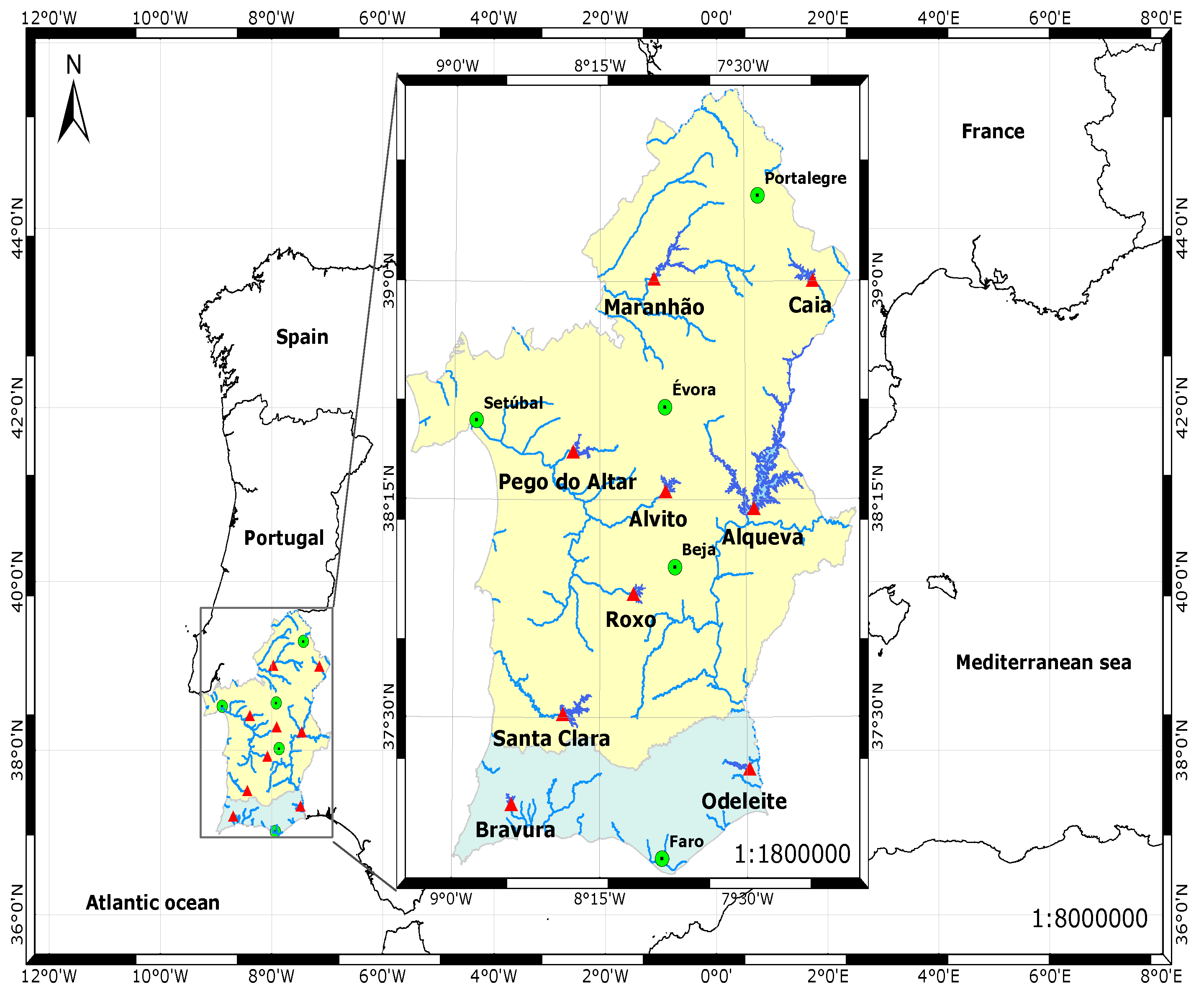
Figure 2.
Schematic representation of meteorological and water temperature floating stations.
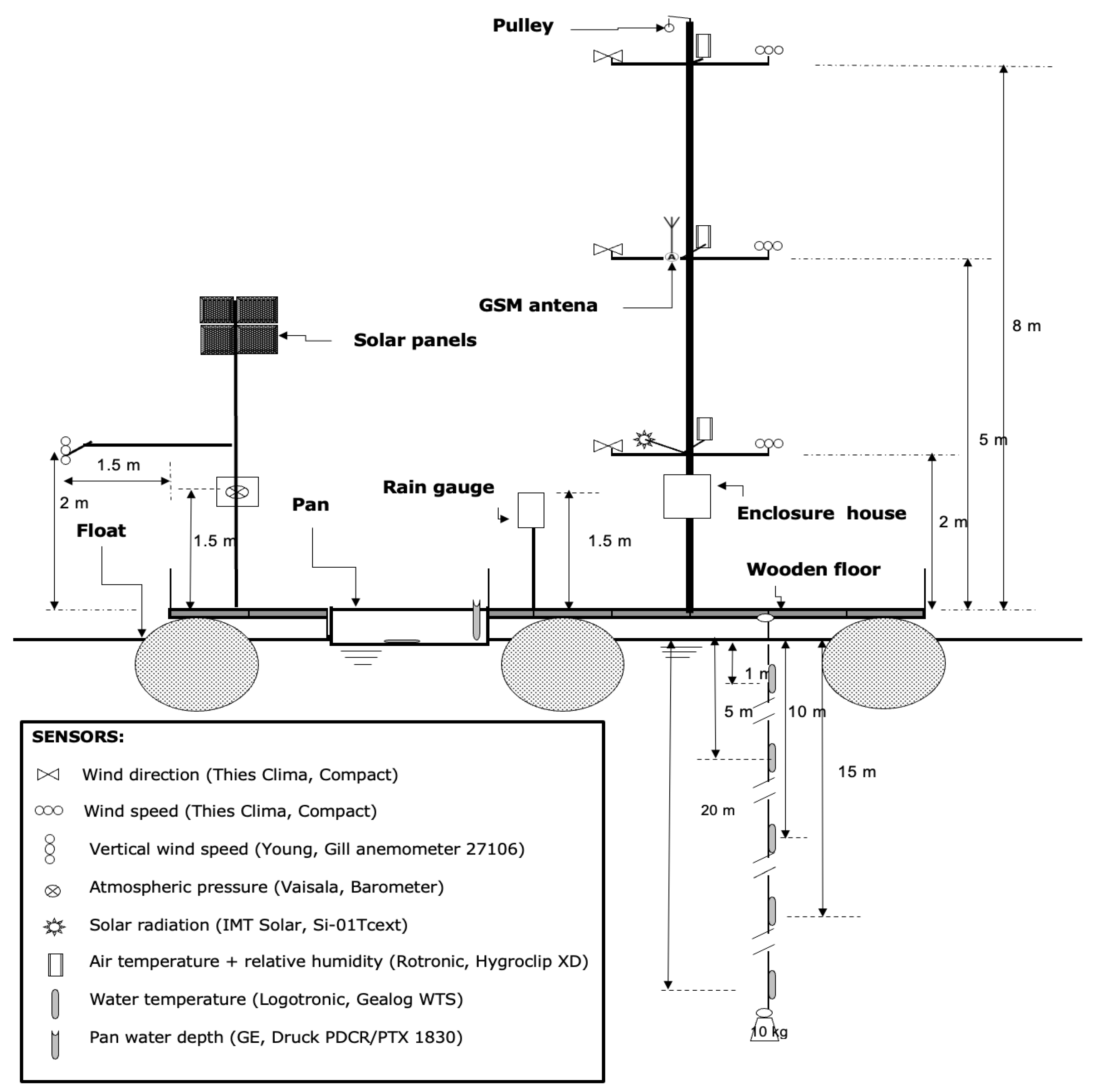
Figure 3.
Annual cycle (left) and daily mean data (right) of air temperature (Ta), water surface temperature (Ts), air relative humidity (RH), wind speed (U2) and incoming solar radiation (Qs) measured at 2 meters high. The 14 days forward moving average was obtained considering the data from all reservoirs.
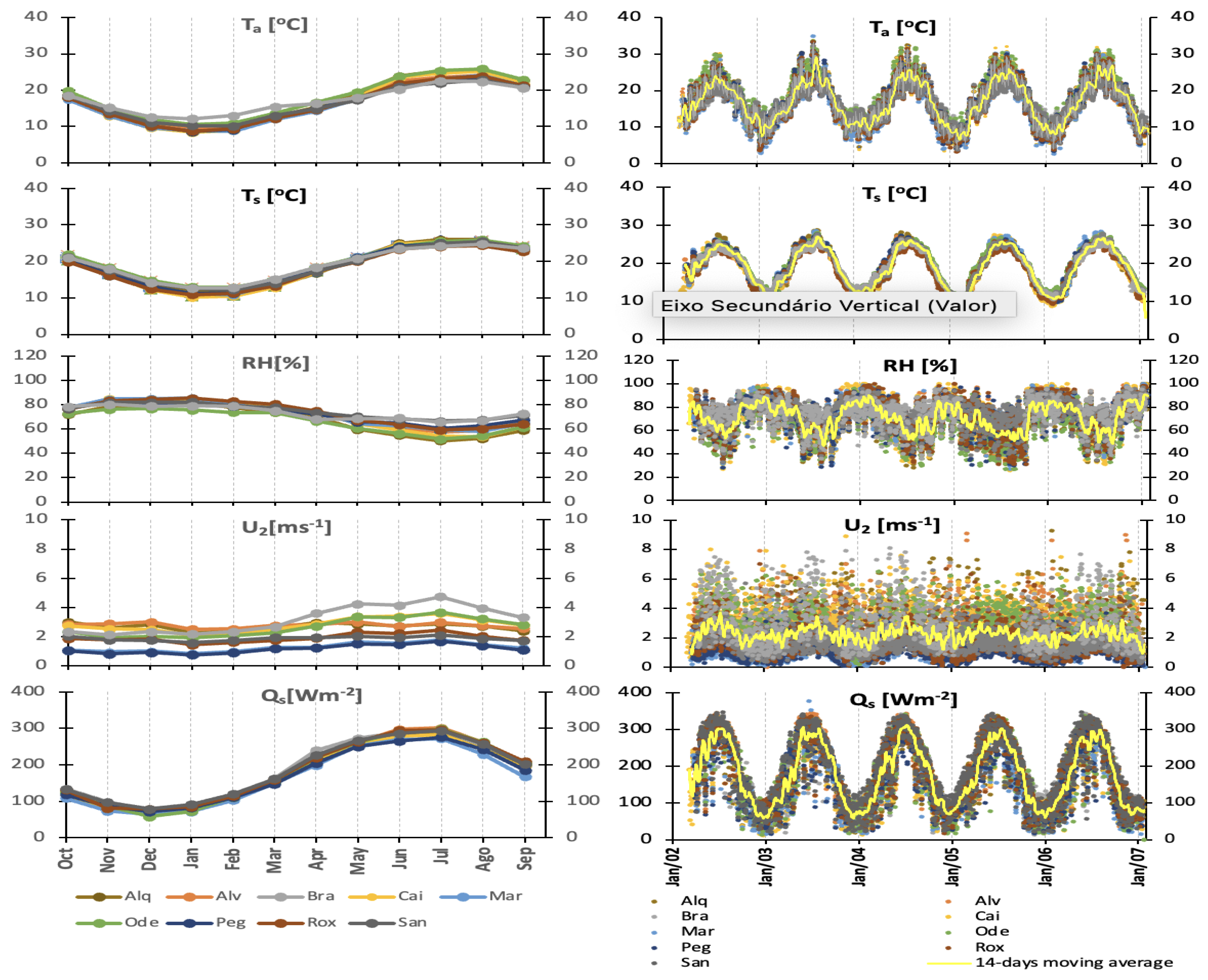
Figure 4.
Daily mean water temperature observed at 1 (), 5 (), 10 (), 15 () and 20 () meters depth in the reservoirs (on left) and corresponding annual cycle (on right). The gaps in the graphics indicate periods of missing data resulting from equipment failures.
Figure 4.
Daily mean water temperature observed at 1 (), 5 (), 10 (), 15 () and 20 () meters depth in the reservoirs (on left) and corresponding annual cycle (on right). The gaps in the graphics indicate periods of missing data resulting from equipment failures.
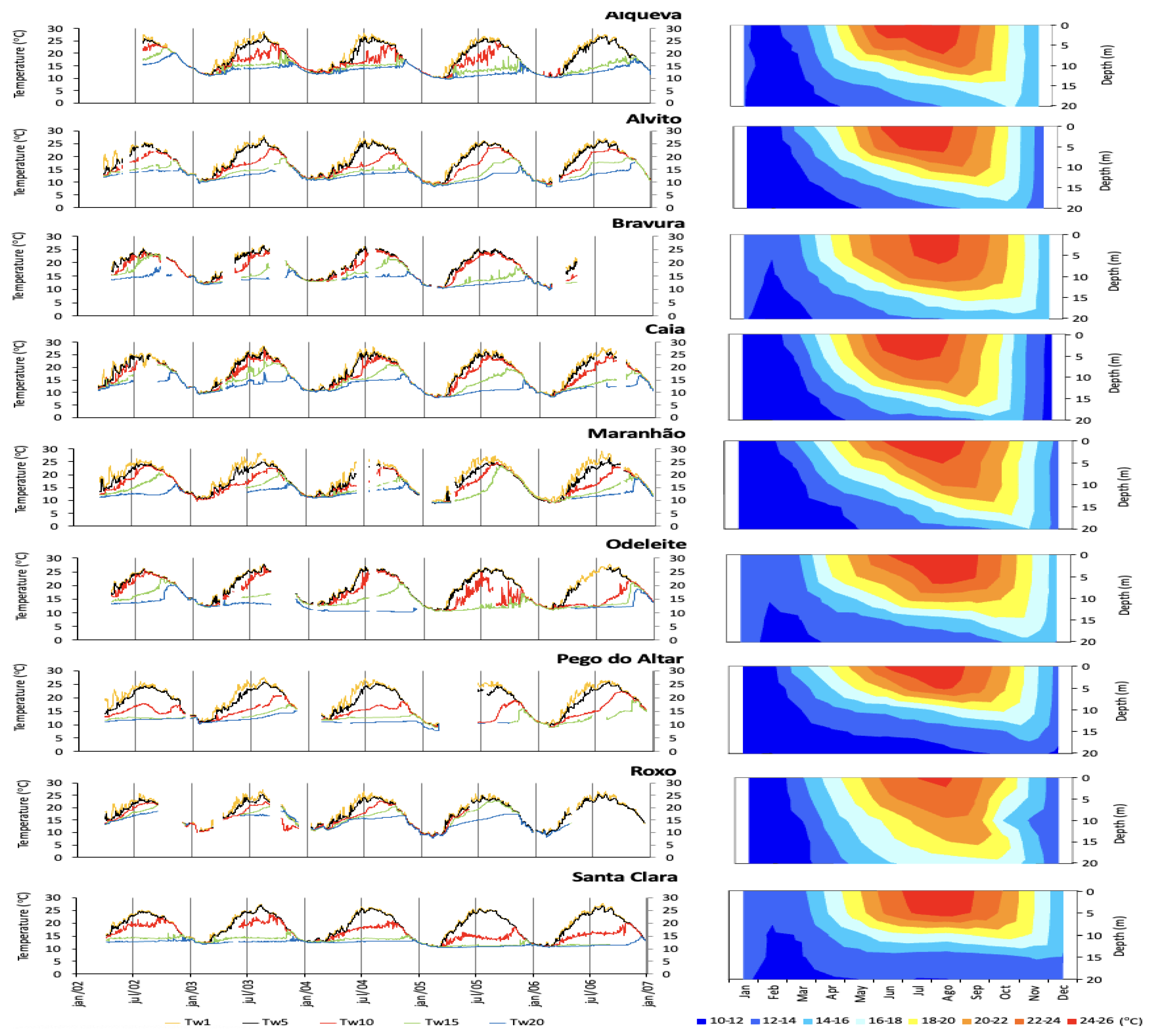
Figure 5.
Monthly energy balance components in reservoirs. Net radiation (), heat storage change in the water body (Q), latent heat flux, () and sensible heat flux (H).
Figure 5.
Monthly energy balance components in reservoirs. Net radiation (), heat storage change in the water body (Q), latent heat flux, () and sensible heat flux (H).
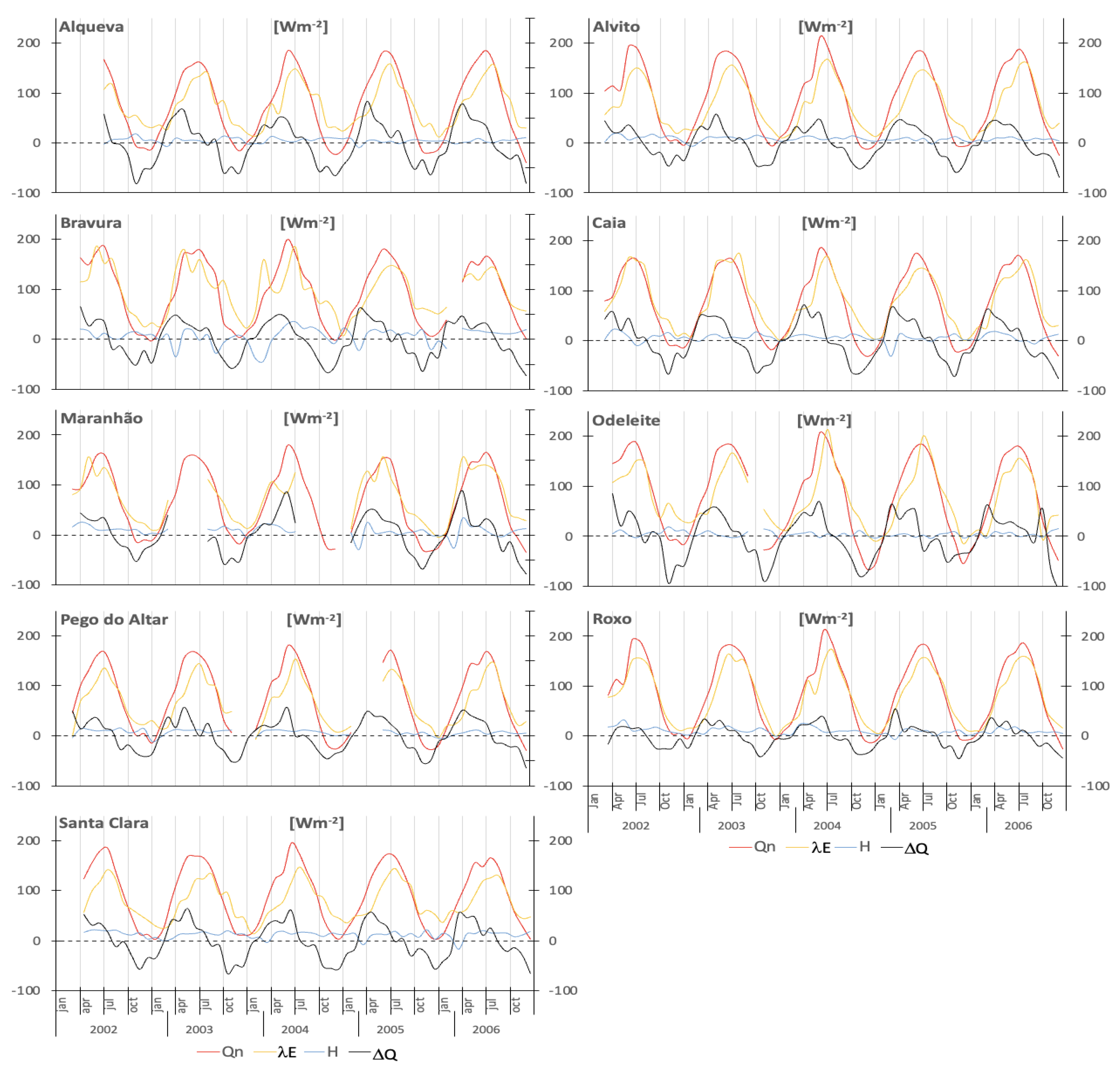
Figure 6.
Monthly energy budget evaporation (bars) and the annual cycle of mean (circles), maximum (squares), and minimum (triangles) values.
Figure 6.
Monthly energy budget evaporation (bars) and the annual cycle of mean (circles), maximum (squares), and minimum (triangles) values.
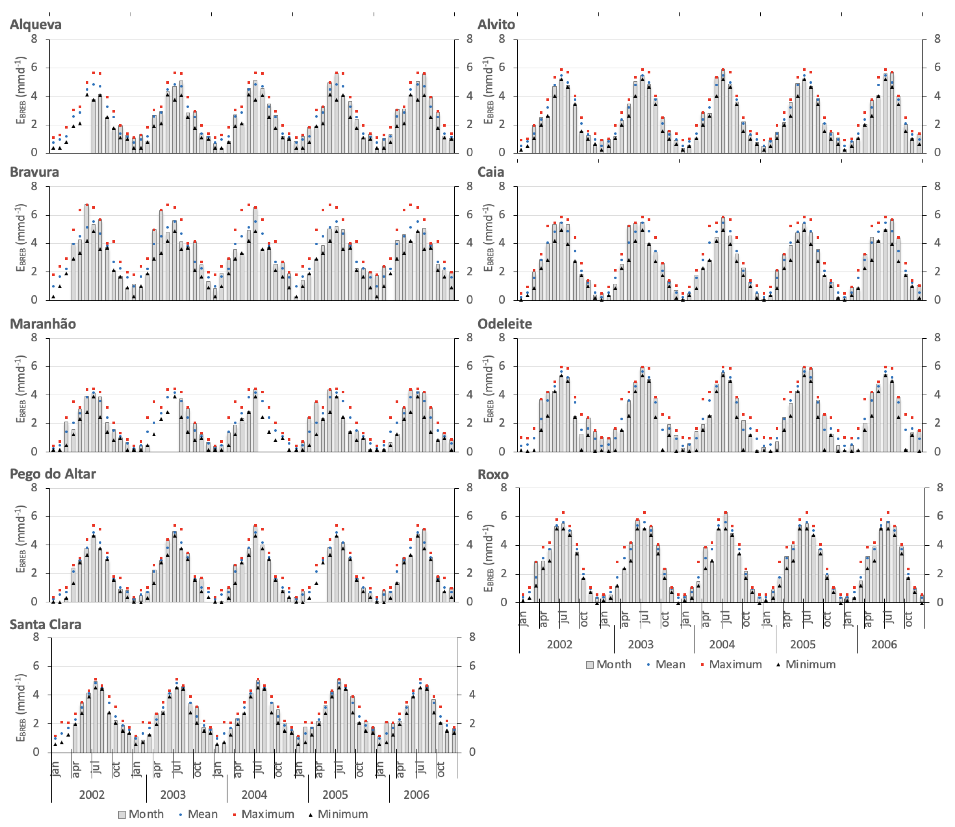
Figure 7.
Monthly mean evaporation estimated by the BREB method.
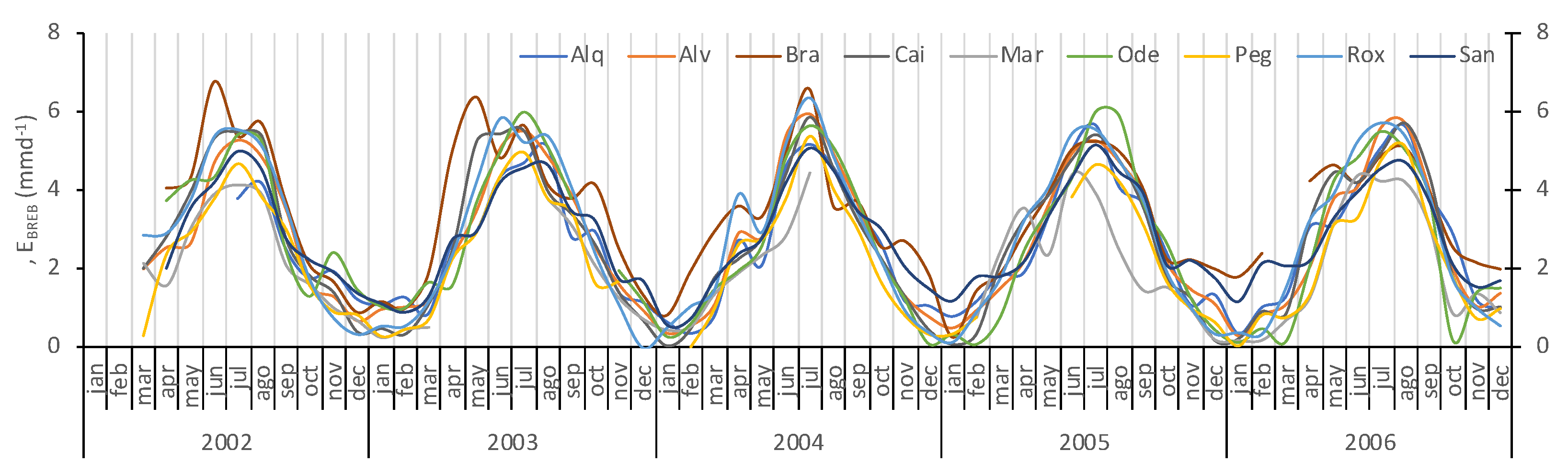
Figure 8.
Spatial distribution of monthly mean (a to l) and seasonal mean (m and n) reservoir evaporation in southern Portugal.
Figure 8.
Spatial distribution of monthly mean (a to l) and seasonal mean (m and n) reservoir evaporation in southern Portugal.
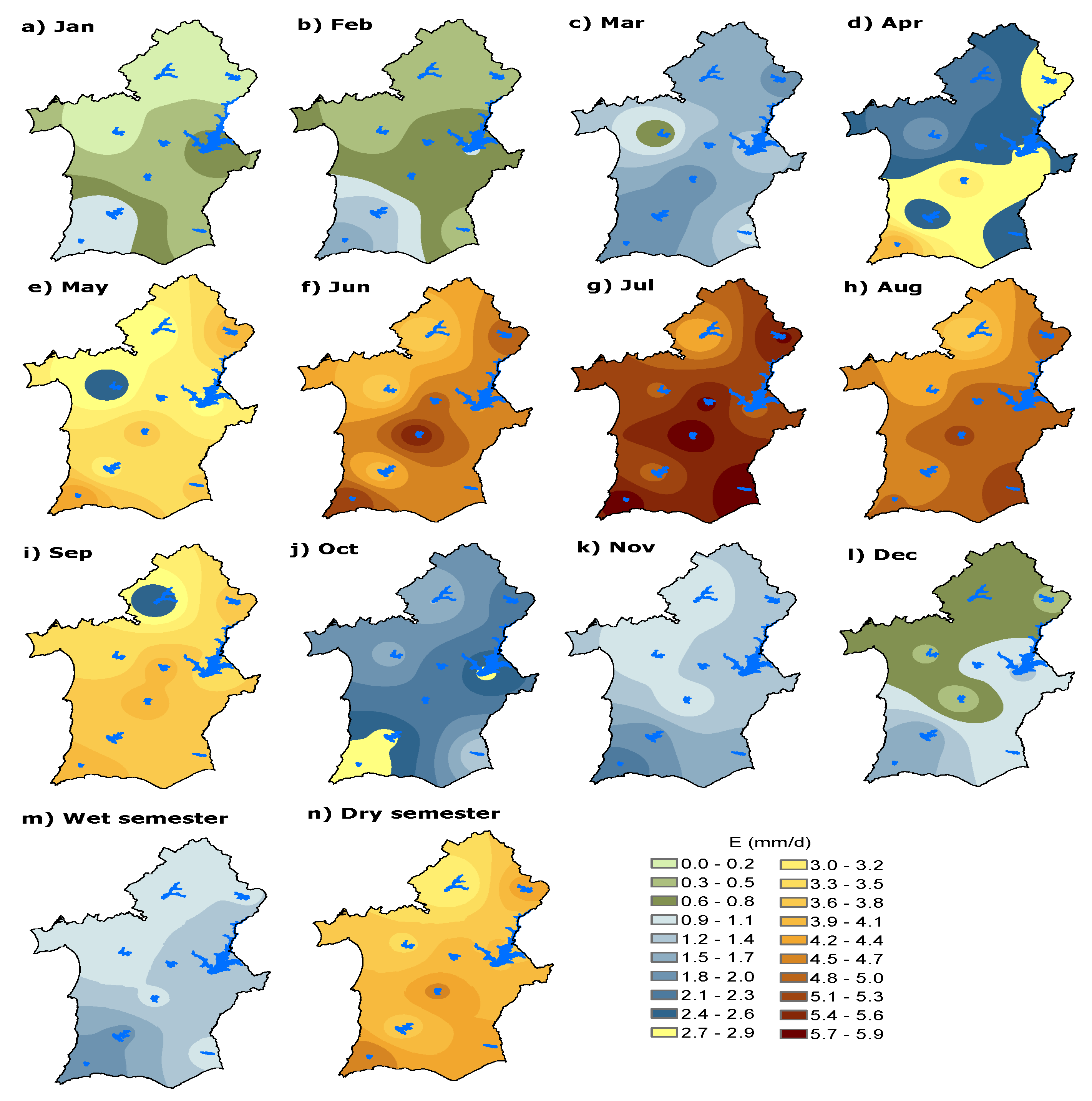
Figure 9.
Spatial distribution of mean annual reservoir evaporation in southern Portugal.
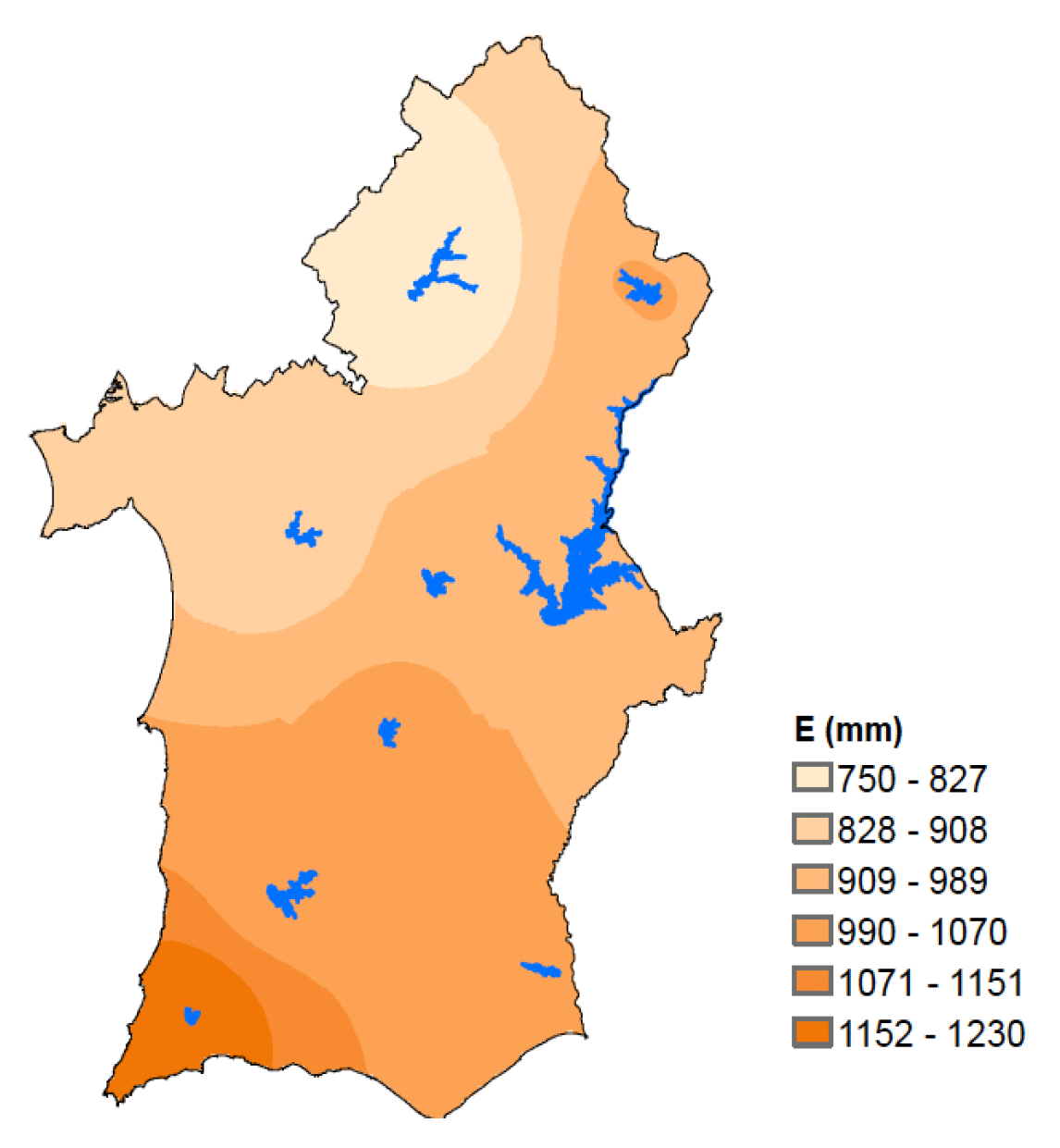
Figure 10.
Evaporation estimated by the 5 indirect methods compared to evaporation calculated by the energy-budget method (), for Alqueva reservoir: Left – trend lines; right – difference for the average monthly evaporation, blue – wet semester; orange – dry semester.
Figure 10.
Evaporation estimated by the 5 indirect methods compared to evaporation calculated by the energy-budget method (), for Alqueva reservoir: Left – trend lines; right – difference for the average monthly evaporation, blue – wet semester; orange – dry semester.
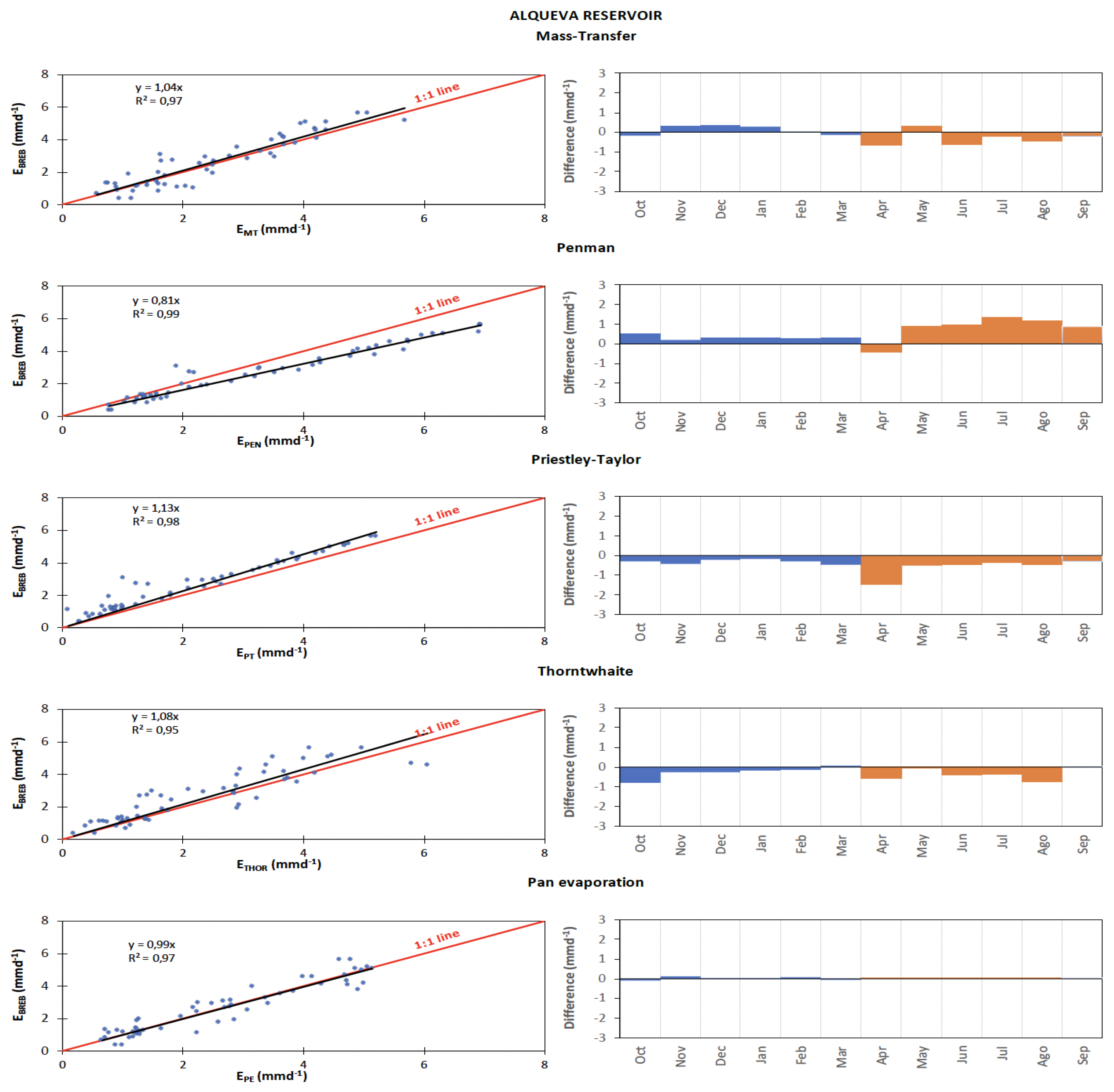
Figure 11.
Seasonal mean and ± standard deviation of the differences between the monthly estimates of the alternate evaporation methods and the BREB method at all reservoirs. The two orange lines display the standard deviation value associated with the BREB daily estimates.
Figure 11.
Seasonal mean and ± standard deviation of the differences between the monthly estimates of the alternate evaporation methods and the BREB method at all reservoirs. The two orange lines display the standard deviation value associated with the BREB daily estimates.
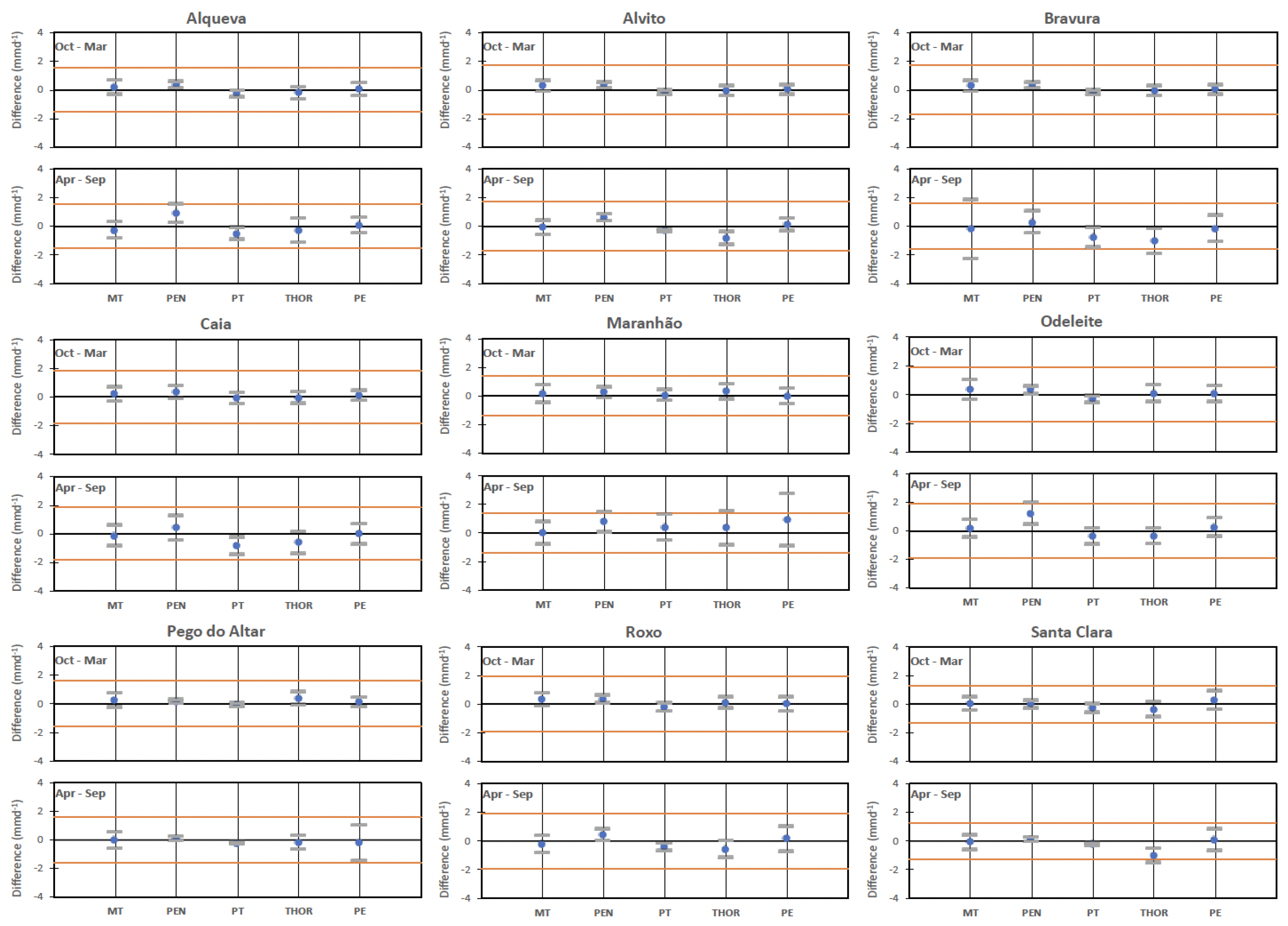
Figure 12.
Taylor diagram for the 9 reservoirs showing the relative Performance of the five evaporation methods compared to the BREB. The RMSE is indicated by pink arcs, the black arc refers to the NSD, and the green contours indicate the R. The five evaporation methods were assigned by letters.
Figure 12.
Taylor diagram for the 9 reservoirs showing the relative Performance of the five evaporation methods compared to the BREB. The RMSE is indicated by pink arcs, the black arc refers to the NSD, and the green contours indicate the R. The five evaporation methods were assigned by letters.
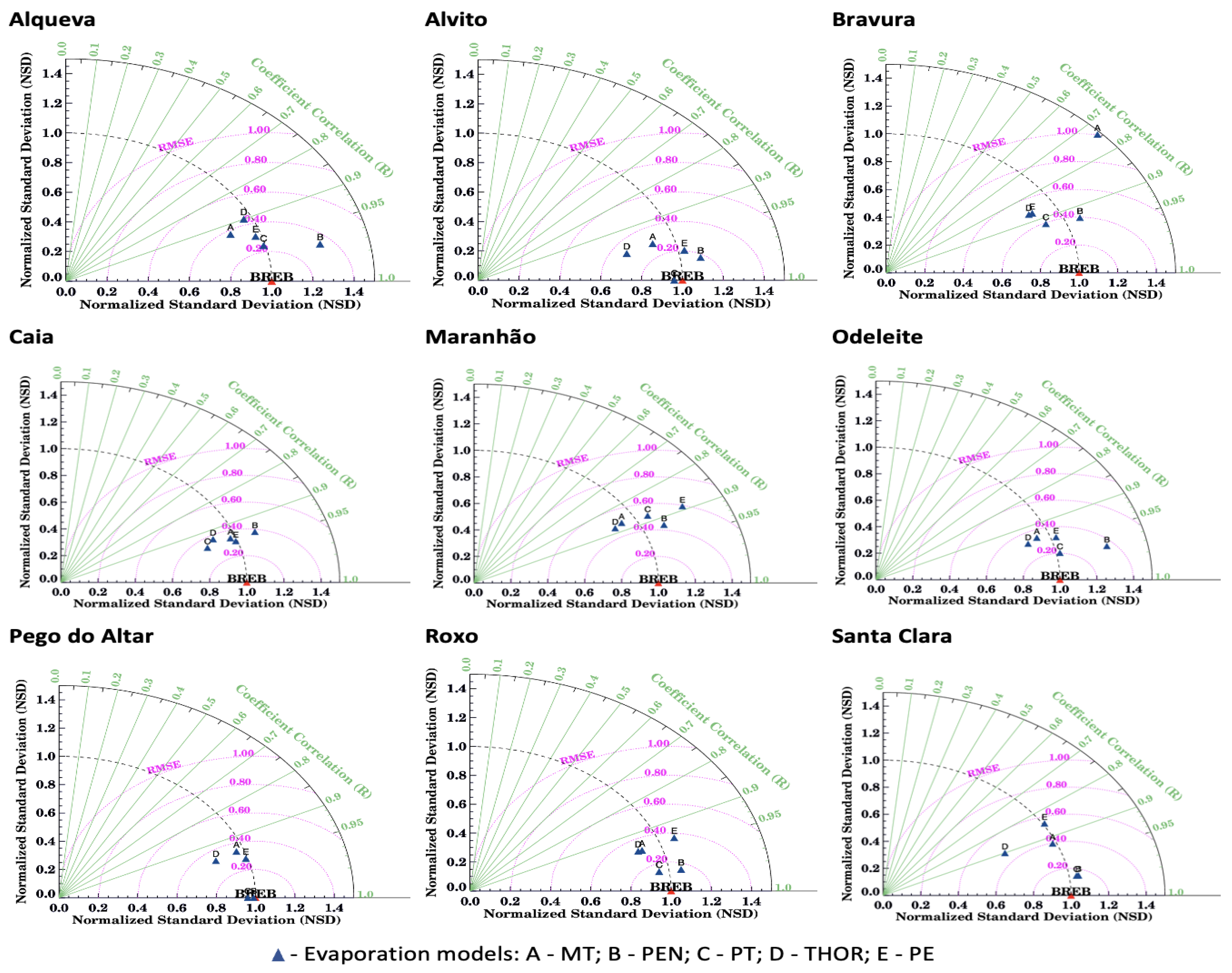

Table 1.
Main reservoir morphometric characteristics.
| Parameter | Reservoirs | ||||||||
|---|---|---|---|---|---|---|---|---|---|
| Alqueva | Alvito | Bravura | Caia | Maranhão | Odeleite | Pego do Altar | Roxo | Sta Clara | |
| NWL (m) | 152.0 | 197.5 | 84.1 | 233.5 | 130.0 | 52.0 | 52.3 | 136.0 | 130.0 |
| V (hm3) | 4150.0 | 132.5 | 34.8 | 192.3 | 205.4 | 130.0 | 94.0 | 96.3 | 485.0 |
| As (km2) | 250.0 | 14.8 | 2.9 | 19.7 | 19.6 | 7.2 | 8.0 | 13.8 | 19.9 |
| Mn depth (m) | 16.6 | 8.9 | 12.2 | 9.8 | 10.5 | 18.1 | 11.8 | 7.0 | 24.4 |
| Mx depth (m) | 77.0 | 32.8 | 34.5 | 37.2 | 44.0 | 41.3 | 37.3 | 27.3 | 71.6 |
| P(km) | 1160.0 | 93.2 | 33.9 | 99.8 | 188.0 | 65.3 | 94.7 | 99.2 | 230.0 |
| L (km) | 83.0 | 7.0 | 5.5 | 12.8 | 25.0 | 18.0 | 15.0 | 4.3 | 21.2 |
| (P/L) | 14.0 | 13.3 | 6.2 | 7.8 | 7.5 | 3.6 | 6.3 | 23.1 | 10.9 |
| Kc (-) | 30.3 | 6.8 | 5.6 | 6.3 | 11.9 | 6.8 | 9.4 | 7.5 | 14.5 |
| Ad (km2) | 55400.0 | 212.0 | 76.8 | 571.0 | 2282.0 | 352.0 | 743.0 | 351.0 | 520.0 |
| Ad/As | 222.0 | 14.0 | 27.0 | 29.0 | 116.0 | 49.0 | 93.0 | 25.0 | 26.0 |
NWL – Normal water level; V – Total reservoir capacity; As – Water surface area; Mn depth – Mean depth; Mx depth – Maximum depth; P – Water surface perimeter; L – Reservoir length; Kc – Compacity coefficient (Gravellius); Ad – Catchment area.
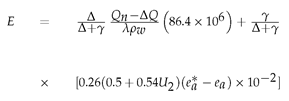
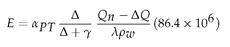
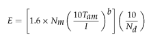
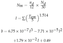
Table 2.
Mathematic formulation of the methods used in the study.
| Method | References | Eq.n. | Equation | Equation terms and parameters |
|---|---|---|---|---|
| BREB | [16]; [17] |
(4) | 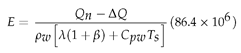 |
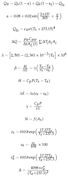 |
| MT | [18,23]; [9] |
(5) |  |
|
| PEN | [24]; [25] |
(6) |  |
|
| PT | [26]; [27] |
(7) |  |
|
| THOR | [28]; [29]; [30] |
(8) |  |
 |
| PE | [31]; [9] |
(9) |  |
The multipliers of 86.4 × 10⁶ that appear in equations are used to convert results into mm d−1. E – Reservoir evaporation rate (mm d−1); - Net radiation (W m−2); - Incoming solar radiation (W m−2); - Surface short wave albedo; - Julian day; - Incoming atmospheric radiation (W m−2); ); - Surface long wave albedo = 0.03; – Emitting long wave radiation from the surface (W m−2); - Water emissivity = 0.97; -Stefan-Boltzmann constant = 5.67 x 10⁻⁸ (W m−2); - Water surface temperature (°C); - Heat storage change in the water body (W m−2); - Density of water = 998 (kg m−2 at 20° C); - Specific heat capacity of water = 4186 (J kg−1 °C−1); - Time interval (s); – Reservoir surface area, a function of reservoir surface elevation and the time (km2); i - Number of layers (1 to 5) where water temperature was measured; - Temperature difference of layer i in two consecutive days (°C); - Thickness of each horizontal layer (m); - Average area of each horizontal layer (km2); - Bowen ratio; H – Sensible heat flux (W m−2); - Latent heat flux (W m−2); - Psychrometric constant (Pa °C−1); - Specific heat capacity at constant pressure = 1006 (J kg−1 °C−1); P - Atmospheric pressure (Pa); - Ratio of molecular weight of water vapour/dry air = 0.622; - Latent heat of vaporization (J kg−1); - Air temperature (°C); - Saturated vapour pressure at water temperature (Pa); - Actual vapour pressure (Pa); RH – Air relative humidity (%); N - Mass transfer coefficient ((mm d−1/(Pa m s−1)); – Water surface area (km2); - Wind speed at 2 meters above the water surface (m s−1); - Slope of the saturated vapour pressure-temperature curve at mean air temperature (Pa °C−1); - Saturated vapour pressure at air temperature (Pa); - Dimensionless proportionality Priestley-Taylor coefficient = 1.26; - Correction factor according to the latitude and time of the year; - Duration of average monthly or daily daylight (h); - Number of days in the month; - Mean monthly air temperature (°C); I - Annual thermal index; b - Polynomial function of the index; – Measured pan evaporation rate (mm d−1), - Pan coefficient.
Table 3.
Statistical descriptors.
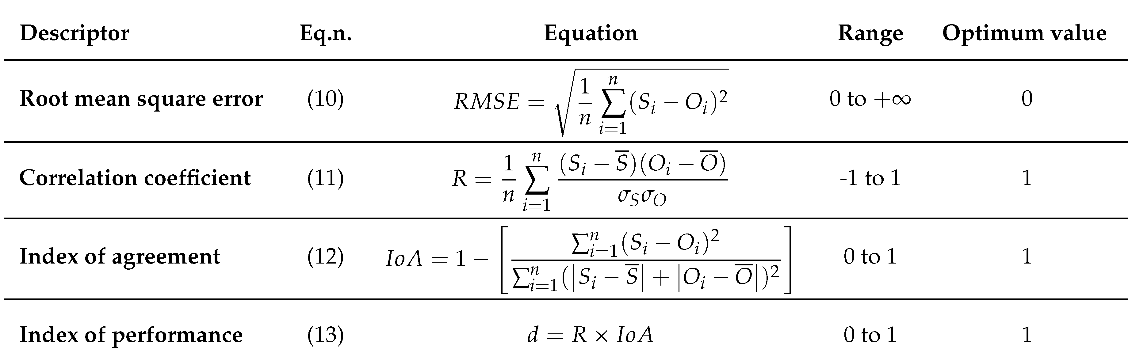 |
Si - Indirect method values; Oi - BREB values; S- Mean of the indirect method values; σS - Standard deviation of the indirect method values; O - Mean of the BREB values; σO - Standard deviation of the BREB values; n - Number of values.
Table 4.
Index of performance, d, classification.
| d value | Performance |
|---|---|
| >0.85 | Excellent |
| 0.76 – 0.85 | Very good |
| 0.66 – 0.75 | Good |
| 0.61 – 0.65 | Average |
| 0.51 – 0.60 | Poor |
| 0.41 – 0.50 | Bad |
| <0.40 | Very bad |
Table 5.
Annual mean values of reservoir energy fluxes (W m−2) and the (%).
| Reservoirs | |||||||||
|---|---|---|---|---|---|---|---|---|---|
| Alqueva | Alvito | Bravura | Caia | Maranhão | Odeleite | Pego do Altar | Roxo | Sta Clara | |
| 314.2 | 317.0 | 320.5 | 310.3 | 313.6 | 316.4 | 315.9 | 317.0 | 320.5 | |
| 402.1 | 399.2 | 402.2 | 399.1 | 399.7 | 404.1 | 400.6 | 399.0 | 402.4 | |
| -87.9 | -82.2 | -81.7 | -88.8 | -86.1 | -87.7 | -84.7 | -82.0 | -81.9 | |
| 162.6 | 169.9 | 173.5 | 161.8 | 154.0 | 168.0 | 159.0 | 169.4 | 173.4 | |
| 74.7 | 87.7 | 91.8 | 73.0 | 67.9 | 80.3 | 74.3 | 87.4 | 91.5 | |
| -0.2 | 0.1 | 0.4 | 0.2 | 1.9 | -0.8 | 0.6 | -1.2 | -0.9 | |
| 74.4 | 76.7 | 96.6 | 79.4 | 74.6 | 77.9 | 65.3 | 79.9 | 79.0 | |
| H | 5.4 | 8.3 | 6.8 | 6.8 | 8.0 | 4.2 | 7.1 | 10.2 | 12.5 |
| 6.5 | -3.0 | 13.1 | 18.4 | 25.2 | 1.2 | -1.8 | 1.7 | -1.0 | |
Net loss of heat in the long-wave radiative balance, , is calculated by
Table 6.
Evaporation estimated by the 5 indirect methods compared to evaporation calculated by the energy-budget method. Annual mean, determination coefficient and maximum and minimum differences in average monthly evaporation for wet and dry semesters (mm d−1).
Table 6.
Evaporation estimated by the 5 indirect methods compared to evaporation calculated by the energy-budget method. Annual mean, determination coefficient and maximum and minimum differences in average monthly evaporation for wet and dry semesters (mm d−1).
| Reservoir | Method | Mean | R2 | MaxB_WS | MinB_WS | MaxB_DS | MinB_DS |
|---|---|---|---|---|---|---|---|
| Alqueva | MT | 2,52 | 0,97 | 0,62 | -0,06 | -0,21 | -0,04 |
| PEN | 3,20 | 0,99 | 0,52 | 0,15 | 0,31 | -0,13 | |
| PT | 2,17 | 0,98 | -0,42 | -0,11 | -0,57 | -0,09 | |
| THOR | 2,30 | 0,95 | -0,29 | -0,04 | -0,16 | 0,03 | |
| PE | 2,60 | 0,96 | 0,35 | 0,01 | 0,06 | 0,00 | |
| Alvito | MT | 2,75 | 0,98 | 0,97 | -0,01 | 0,18 | -0,01 |
| PEN | 3,13 | 1,00 | 0,85 | 0,16 | 0,18 | 0,10 | |
| PT | 2,42 | 1,00 | -0,30 | -0.08 | -0,15 | -0,07 | |
| THOR | 2,20 | 0,98 | 0,47 | 0,01 | -0,24 | -0,16 | |
| PE | 2,72 | 0,99 | -0,16 | 0,02 | 0,02 | 0,02 | |
| Bravura | MT | 3,15 | 0,86 | -0,48 | -0,20 | -0,29 | 0,03 |
| PEN | 3,47 | 0,97 | 1,10 | 0,02 | 0,17 | 0,04 | |
| PT | 2,68 | 0,97 | -0,56 | -0,11 | -0,34 | -0,10 | |
| THOR | 2,53 | 0,94 | 0,84 | 0,08 | -0,46 | -0,07 | |
| PE | 3,12 | 0,95 | 0,92 | 0,04 | -0,45 | -0,17 | |
| Caia | MT | 2,72 | 0,96 | 1,35 | 0,10 | -0,23 | 0,03 |
| PEN | 3,07 | 0,97 | 1,27 | -0,04 | 0,28 | 0,10 | |
| PT | 2,20 | 0,97 | -0,67 | -0,09 | -0,36 | -0,10 | |
| THOR | 2,35 | 0,96 | 0,37 | 0,01 | -0,39 | -0,02 | |
| PE | 2,74 | 0,97 | 0,73 | 0,00 | 0,11 | 0,01 | |
| Maranhão | MT | 2,06 | 0,97 | 2,23 | -0,07 | -0,18 | 0,02 |
| PEN | 2,52 | 0,95 | 0,97 | -0.06 | 1,07 | 0,14 | |
| PT | 2,22 | 0,93 | -0,93 | 0,01 | 1,15 | -0,01 | |
| THOR | 2,22 | 0,93 | 2,08 | 0,38 | 0,37 | 0,04 | |
| PE | 2,54 | 0,76 | 0,45 | -0,01 | 0,65 | 0,00 | |
| Odeleite | MT | 2,90 | 0,96 | 3,15 | -0,02 | 0,13 | 0,00 |
| PEN | 3,45 | 0,99 | 1,49 | 0,11 | 0,37 | 0,23 | |
| PT | 2,32 | 0,98 | -1,33 | -0,50 | -0,23 | 0,00 | |
| THOR | 2,52 | 0,97 | 2,08 | 0,22 | -0,17 | -0,08 | |
| PE | 2,83 | 0,97 | 3,26 | 0,00 | 0,12 | 0,03 | |
| Pego do Altar | MT | 2,37 | 0,96 | 1,83 | -0,01 | 0,21 | 0,00 |
| PEN | 2,39 | 1,00 | 1,15 | 0,07 | 0,04 | -0,02 | |
| PT | 2,10 | 1,00 | -0,44 | -0,09 | -0,13 | -0,06 | |
| THOR | 2,27 | 0,97 | 1,67 | -0,01 | -0,13 | -0,01 | |
| PE | 2,30 | 0,97 | 0,85 | 0,02 | -0,20 | 0,00 | |
| Roxo | MT | 2,82 | 0,97 | 1,61 | -0,22 | -0,25 | 0,00 |
| PEN | 3,16 | 0,99 | 1,26 | -0,01 | 0,14 | 0,05 | |
| PT | 2,46 | 0,99 | -0,38 | -0,11 | -0,22 | -0,07 | |
| THOR | 2,54 | 0,97 | 0,62 | -0,21 | -0,40 | -0,01 | |
| PE | 2,89 | 0,96 | 0,29 | 0,00 | 0,06 | 0,00 | |
| Santa Clara | MT | 2,71 | 0,97 | 0,23 | 0,00 | -0,09 | -0,01 |
| PEN | 2,82 | 1,00 | -0,16 | 0,00 | 0,04 | 0,00 | |
| PT | 2,48 | 0,99 | -0,45 | -0,09 | -0,17 | -0,04 | |
| THOR | 2,04 | 0,97 | -0,39 | -0,06 | -0,35 | -0,14 | |
| PE | 2,87 | 0,95 | 1,1 | 0,03 | -0,01 | 0,03 |
MaxB_WS – Maximum bias in wet semester; Min_Bws – Minimum bias in wet semester; MaxB_DS – Maximum bias in dry semester; MinB_DS – Minimum bias in dry semester.
Table 7.
Mass transfer coefficient, N (mm d−1)/(Pa m s−1) and its relationship with water surface area, (km2).
Table 7.
Mass transfer coefficient, N (mm d−1)/(Pa m s−1) and its relationship with water surface area, (km2).
| Reservoirs | N | |||
| Alqueva | 250 | 0.00092 | 0.88 | |
| Alvito | 14.8 | 0.00101 | 0.91 | |
| Bravura | 2.85 | 0.00104 | 0.60 | |
| Caia | 19.7 | 0.00990 | 0.91 | |
| Maranhão | 19.6 | 0.00158 | 0.71 | |
| Odeleite | 7.2 | 0.00095 | 0.90 | |
| Pego do Altar | 7.98 | 0.00176 | 0.83 | |
| Roxo | 13.78 | 0.00157 | 0.90 | |
| Santa Clara | 19.86 | 0.00159 | 0.79 | |
| Lake Mirror | 0.15 | 0.00164 | ||
| Lake Hefner | 10.5 | 0.00095 | ||
| Lake Mead | 640 | 0.00118 | ||
| Lake Vergoritis | 33.5 | 0.00143 |
Table 8.
Statistical descriptors of monthly evaporation (mm d−1) and methods performance, for all reservoirs.
Table 8.
Statistical descriptors of monthly evaporation (mm d−1) and methods performance, for all reservoirs.
| Reservoir | Method | RMSE | R | IOA | d | Performance |
|---|---|---|---|---|---|---|
| Alqueva | MT | 0,57 | 0,93 | 0,96 | 0,89 | Excellent |
| PEN | 0,80 | 0,98 | 0,95 | 0,92 | Excellent | |
| PT | 0,57 | 0,97 | 0,96 | 0,94 | Excellent | |
| THOR | 0,73 | 0,90 | 0,94 | 0,84 | Very Good | |
| PE | 0,49 | 0,95 | 0,97 | 0,92 | Excellent | |
| Alvito | MT | 0,48 | 0,96 | 0,98 | 0,94 | Excellent |
| PEN | 0,49 | 0,99 | 0,98 | 0,98 | Excellent | |
| PT | 0,32 | 1,00 | 0,99 | 0,99 | Excellent | |
| THOR | 0,75 | 0,97 | 0,94 | 0,91 | Excellent | |
| PE | 0,39 | 0,98 | 0,99 | 0,96 | Excellent | |
| Bravura | MT | 1,60 | 0,74 | 0,82 | 0,61 | Average |
| PEN | 0,65 | 0,93 | 0,96 | 0,89 | Excellent | |
| PT | 0,92 | 0,92 | 0,90 | 0,83 | Very Good | |
| THOR | 1,16 | 0,87 | 0,83 | 0,72 | Good | |
| PE | 0,78 | 0,87 | 0,93 | 0,81 | Very Good | |
| Caia | MT | 0,64 | 0,94 | 0,97 | 0,91 | Excellent |
| PEN | 0,75 | 0,94 | 0,96 | 0,91 | Excellent | |
| PT | 0,82 | 0,95 | 0,94 | 0,89 | Excellent | |
| THOR | 0,77 | 0,93 | 0,95 | 0,88 | Excellent | |
| PE | 0,56 | 0,95 | 0,98 | 0,93 | Excellent | |
| Maranhão | MT | 0,69 | 0,87 | 0,93 | 0,81 | Very Good |
| PEN | 0,77 | 0,92 | 0,93 | 0,85 | Excellent | |
| PT | 0,72 | 0,88 | 0,94 | 0,83 | Very Good | |
| THOR | 0,61 | 0,88 | 0,93 | 0,82 | Very Good | |
| PE | 0,90 | 0,89 | 0,90 | 0,80 | Very Good | |
| Odeleite | MT | 0,64 | 0,94 | 0,97 | 0,91 | Excellent |
| PEN | 1,01 | 0,98 | 0,94 | 0,92 | Excellent | |
| PT | 0,57 | 0,98 | 0,98 | 0,95 | Excellent | |
| THOR | 0,62 | 0,95 | 0,97 | 0,92 | Excellent | |
| PE | 0,60 | 0,95 | 0,97 | 0,93 | Excellent | |
| Pego do Altar | MT | 0,53 | 0,94 | 0,97 | 0,90 | Excellent |
| PEN | 0,16 | 1,00 | 1,00 | 0,99 | Excellent | |
| PT | 0,24 | 1,00 | 0,99 | 0,99 | Excellent | |
| THOR | 0,51 | 0,95 | 0,97 | 0,92 | Excellent | |
| PE | 0,41 | 0,96 | 0,98 | 0,94 | Excellent | |
| Roxo | MT | 0,59 | 0,95 | 0,97 | 0,93 | Excellent |
| PEN | 0,50 | 0,99 | 0,98 | 0,97 | Excellent | |
| PT | 0,45 | 0,99 | 0,98 | 0,97 | Excellent | |
| THOR | 0,68 | 0,95 | 0,96 | 0,91 | Excellent | |
| PE | 0,70 | 0,94 | 0,97 | 0,91 | Excellent | |
| Santa Clara | MT | 0,49 | 0,92 | 0,96 | 0,89 | Excellent |
| PEN | 0,22 | 0,99 | 0,99 | 0,98 | Excellent | |
| PT | 0,37 | 0,99 | 0,98 | 0,97 | Excellent | |
| THOR | 0,95 | 0,90 | 0,80 | 0,72 | Good | |
| PE | 0,68 | 0,85 | 0,91 | 0,78 | Very Good |
Disclaimer/Publisher’s Note: The statements, opinions and data contained in all publications are solely those of the individual author(s) and contributor(s) and not of MDPI and/or the editor(s). MDPI and/or the editor(s) disclaim responsibility for any injury to people or property resulting from any ideas, methods, instructions or products referred to in the content. |
© 2025 by the authors. Licensee MDPI, Basel, Switzerland. This article is an open access article distributed under the terms and conditions of the Creative Commons Attribution (CC BY) license (http://creativecommons.org/licenses/by/4.0/).
Copyright: This open access article is published under a Creative Commons CC BY 4.0 license, which permit the free download, distribution, and reuse, provided that the author and preprint are cited in any reuse.


