Submitted:
09 September 2025
Posted:
16 September 2025
You are already at the latest version
Abstract
In this paper, we study existence and stability of solutions for a class of new coupled systems of fuzzy fractional partial differential equations involving Caputo--Katugampola and generalized Hukuhara (gH-) type derivatives, which provides a solid theoretical foundation and effective analytical tools for scientific research and engineering practice to address highly complex, uncertain, and memory-dependent interacting systems. Under some suitable assumptions that break through the limitations of traditional Lipschitz conditions, existence of classical solutions of the coupled systems is strictly proved by innovatively applying Schauder fixed point theorem. Furthermore, the existence of two kinds of gH-type weak solutions is confirmed by constructing typical examples. Further, stability of the fuzzy fractional partial differential coupled systems is analyzed based on Ulam--Hyers stability theory.
Keywords:
existence theorem
; Ulam–Hyers stabilization
; fuzzy fractional partial differential symmetry coupled system
; Caputo–Katugampola and generalized Hukuhara type derivative
; Schauder fixed point theorem
MSC: 47H10; 35A01; 35D30; 35R11; 26A33
1. Introduction
Based on Caputo–Katugampola (C-K) fractional derivative approach due to Katugampola [1], which expand the theoretical framework of fractional differential via unifying Riemann–Liouville and Hadamard fractional derivatives, Singh et al. [2] investigated the following prey-predator fractional-order biological population model with carrying capacity and understanding their interactivity:
which contributes significantly to ecological community, where and denote the population densities of the prey and predator, respectively, represents the growth rate of the prey, the carrying capacity, and the competitive interaction rates, and the growth rate of the predator; all these coefficients are positive constants.
We remark that in recent years, C-K fractional derivative has been widely adopted owing to its capability to capture local differential and integral characteristics and provided a framework for handling systems with fractional exponents. It is especially applicable to modeling and analyzing systems exhibiting fractional dynamic behaviors [3,4], which laid an important foundation for the follow-up research. Since then, scholars have carried out systematic research on C-K derivative. In fact, with the in-depth study of complex systems, the traditional integer-order derivative model shows limitations in describing processes with memory, heredity or nonlocal characteristics, which promotes the development of fractional partial differential equations (FPDEs) [5], which can describe the dynamic evolution of natural phenomena [6] and model the evolution process of physical quantities with space and time in multivariable systems [7]. At the same time, the successful application of this mathematical tool in noise suppression [8], biological engineering [9], physical science [10] and other fields further promotes the deep integration of the theoretical development of FPDEs and practical problems.
On the other hand, biodiversity constitutes the most fundamental attribute of an ecosystem. Nevertheless, prior investigations predominantly centered on the survival and proliferation of individual species, thereby overlooking the competitive dynamics engendered by the coexistence of multiple species. Such mutual interrelations are defined as “coupling” [11] when two or more entities engage in reciprocal interaction and influence. As noted by Ding et al. [12], coupling mechanisms are capable of effectively characterizing the interaction dynamics between two competing species in ecological systems. A representative instance of such coupled structures is the following elliptic system [13]:
where , and is a smooth bounded domain, this system possesses significant capability for capturing the intrinsic dynamics of ecosystems. Furthermore, Zhang et al. [14] applied the fuzzy fractional coupled partial differential equation of Caputo derivative to the initial value problem, and established existence theory of solutions under the gH-type derivative framework. Muatjetjeja et al. [15] conducted a comprehensive Noether symmetry analysis of a generalized coupled Lane-Emden-Klein-Gordon-Fock system with central symmetry.
It is well known that practical engineering systems often have to face issues such as parameter uncertainties, measurement noise, or model inaccuracies. The deterministic framework of traditional fractional-order models is difficult to fully accommodate these challenges, while the introduction of fuzzy theory provides an effective approach to address such uncertainty problems [16,17]. Osman [18] proposed the fuzzy Adomian decomposition method and the modified Laplace decomposition method, successfully solved the fuzzy fractional Navier-Stokes equations, and developed the fuzzy Elzaki transform to deal with the linear-nonlinear Schrodinger equation. Pandey et al. [19] realized efficient numerical approximation of variable-order fuzzy partial differential equations (PDEs) by using Bernstein spectral technique. Mazandarani [20] solved the numerical solution problem of fuzzy fractional initial value problem by improving the fractional Euler method. Furthermore, employing Caputo’s definition of fractional derivatives and gH-difference sets, Singh et al. [21] described fuzzy differential equations and discussed a numerical solution method for fuzzy fractional differential equations with fuzzy fractional counterparts using power series approximation and Taylor’s theorem. It is worth mentioning that Pythagorean fuzzy fractional calculus provides a new paradigm for complex system analysis by virtue of its strong uncertainty modeling ability. For example, Akram et al. [22] successfully analyzed the fractional-order fuzzy wave equation by means of multivariate Pythagorean fuzzy Fourier transform. Baleanu et al. [23] analyzed stability of differential equations under such derivatives by combining Adomian polynomials and fractional Taylor series. Hoa et al. [24] constructed analytical solutions of C-K fuzzy fractional differential equations by the solution of fuzzy integer order differential equation, and verified existence and uniqueness of the solution under the generalized Lipschitz condition. These results significantly enrich the theory and application boundary of fractional calculus.
Since then, researchers have investgated the symmetry coupled systems from various aspects. In the fuzzy fractional population dynamics model, stability condition reveals the long-term evolution trend of species number under fractal habitat and fuzzy environmental carrying capacity, and guides the protection strategy of endangered species. Wang et al. [25] constructed a fractional predator-prey model, and characterized the fractal characteristics of habitat by Caputo fractional derivative. We note that the stability analysis shows that the change of fractional order will significantly affect the stability of population equilibrium point. For different equations, the stability of the solution is not the same. By using Banach contraction principle and Krasnoselskii fixed point theorem, Ali et al. [26] obtained Ulam’s stability of solutions for symmetry coupled systems of fractal fractional differential equations.
where FD is the Caputo fractional derivative and , , and are continuous functions. Andrs et al. [27] studied Ulam–Hyers stability (U-HS) of a class of elliptic PDEs,
which are defined on a bounded domain with Lipschitz boundary by using the direct technique and the abstract method of Picard operator.
Moreover, in the study of calculus theory, Lipschitz condition has long been the core premise of classical results. However, in practical problems, due to complex nonlinear and non-smooth characteristics of the systems, its applicability is limited [28]. Long et al. [29] introduced Schauder-type nonlinear substitution technique to deal with fuzzy-valued continuous functions that do not satisfy Lipschitz condition. By bypassing the traditional dependence on the local smoothness of the function and using the compactness condition of the topological fixed point theory, the second existence result of two kinds of gH-weak solutions for special coupled systems was proved, which expands the scope of application of the theory and provides a more flexible tool for mathematical modeling of complex systems. On this basis, Zhang et al. [14] proved existence of two kinds of gH-weak solutions of coupled fractional equations by the same method, which promoted the development of multi-scale symmetry coupled system theory. In fact, the strict requirements of Lipschitz conditions on the smoothness of functions make it difficult to cover a large number of non-ideal situations in practice. Thus, we consider the related problems without Lipschitz conditions.
Inspired by the previous work [2,14,27], to enhance the ability of system (2) to capture the intrinsic dynamic characteristics of ecological systems, particularly slow diffusion behavior and historical uncertainty effects, we make improvements, introducing C-K gH-type differentiable operator to the left-hand side of (2), more specifically defining the right-hand side, and imposing fuzzy initial conditions. Let M is a fuzzy number space, is a space of fuzzy number , which has the property that the function is continuous with respect to Hausdorff metric on [0, 1], where is -level set of . Thus, we will consider the following symmetry coupled system of fuzzy fractional partial differential equations (FFPDEs) with C-K gH-type differentiability:
for any and , , is a C-K gH-type derivative operator with the fractional order and and are continuous, is a real number. What is noteworthy is that and of (3) suppose the existence of Hukuhara (H-) difference and gH-type difference.
Remark 1.
There are the following points to note:
Consequently, the system (3) are entirely novel and merit in-depth study.
The rest of this paper is as follows: In Section 2, some necessary concepts and other necessary conditions are given. By using Schauder fixed point theorem, existence of two kinds of gH-weak solutions of equation (3) are proved in Section 3. In Section 4, a numerical example is presented. U-HS of the solutions of the symmetry coupled system (3) is proposed in Section 5. Finally, some conclusions and future work are discussed.
2. Preliminaries
In this section, we will define the fractional integral and C-K gH-derivative for fuzzy-valued multivariate functions, and introduce the theory of relative compactness in fuzzy number space. It should be noted that some of these concepts have been more thoroughly explored in [2,12,30].
Definition 1
([14]). Denote M as the space of fuzzy number on , which is a mapping satisfying normal, fuzzy convex, upper semi-continuous, and compactly supported properties. The ϱ-level set of fuzzy number ϑ are defined by:
where cl denotes the closure of the sets and is the support of ϑ.
It is evident that the -level set of the fuzzy number is a closed and bounded interval , where denotes the left-hand endpoint of , and denotes the right-hand endpoint. The diameter of the -level set of is defined as . The highest measure on M is expressed as
where . In , the supremum metric D is taken into account
Thus, and are complete metric spaces. For all , and any , by [31], we know that
where is H-difference of fuzzy numbers and . We suppose that the H-difference always exists. For , the space is defined as the collection of fuzzy numbers that are continuous with respect to the Hausdorff metric (abbreviated as -continuous). According to [32,33], the fuzzy number spaces M and are semilinear spaces possessing the cancellation property. Equipped with metric , both M and form complete metric semilinear spaces. Consequently, the set of fuzzy-valued continuous functions inherits completeness, thereby constituting a Banach semilinear space with the cancellation property. Meanwhile, is defined as the Lebesgue integrable space for fuzzy-valued continuous functions.
For any positive real number r, the closed sphere in the metric space consists of all fuzzy numbers satisfying . Here, the metric D is defined by (6), and is given by for all , where if , and otherwise.
Lemma 1
([2]). For all , the following properties hold:
- (i)
- .
- (ii)
- If and hold, then .
- (iii)
- If exist, then hold and .
- (iv)
- If and are defined, then is defined and satisfies .
- (v)
- If exists, then so does , and we have .
Definition 2
([34]). Let and be a fuzzy-valued mapping. Then f is said to be order gH-type differentiable with respect to x at if the following conditions hold:
- (i)
- f is gH-type differentiable of all orders from 1 to at .
- (ii)
- There exists an element such that for all sufficiently small with , the gH-difference exists, and the following limit holdswhere the gH-type difference , as defined in([35]), satisfiesIn this case, is called the ι-order gH-type derivative of f with respect to x at .
Remark 2.
By Definition 2, the higher-order fuzzy gH-type partial derivatives with respect to y are similarly defined. When , the equation (8) simplifies to
representing the first-order partial derivative of f at with respect to x.
Definition 3
([36]). Let , , and . For and , let , then the mixed Riemann–Liouville fractional integral of orders α for fuzzy-valued multivariable function is defined as:
Definition 4
([13]). the mappings f: and g: are said to be jointly continuous at the point if for every , there exists such that whenever , the following inequalities hold:
, .
For all , define
where , , and are given functions such that and exist. Then define the function spaces:
where and are defined by (12)
For = 0,1,2, denote by the collection of all functions , i=1,2 that possess partial gH-type derivatives up to order m with respect to x and up to n with respect to y in the domain .
Definition 5
([36]). Let , and . Then the C-K gH-type derivative of order α with respect to x and y for the function f is defined by
where the right-hand expression is required to be well-defined, with .
Particularly, we need to distinguish two cases corresponding to and in (9) for any , as follows:
(i) A function satisfies the condition of C-K gH-type differentiability of order concerning x and y if acts as a gH-type derivative of type (i.e., with k = 1 in (3)) at the point . This property is denoted by .
(ii) is -C-K gH-type differentiable of order with respect to x and y when serves as a gH-type derivative of type (i.e., where k = 2 in (3)) at , For this, the notation is used.
Definition 6
([30]). For a subset , S is equicontinuous at if the following holds: for all , there exists such that for each and , implies . We state that S is equicontinuous if S is equicontinuous at every .
Definition 7
([30]). A subset is said to be compactly supported if for every fuzzy number , there exists a compact set such that the support of w, denoted , is contained in K.
Definition 8
([30]). A subset is defined as level-equicontinuous at when the following holds: for all , there exists , such that implies Hausdorff metric for each . Additionally, S is termed level-equicontinuous on if S is level-equicontinuous at every .
Definition 9
([13]). Let and be -continuous fuzzy number spaces. A continuous mapping is called a compact operator if it maps every bounded subset to a relatively compact set in , i.e., the closure forms a compact subset of .
Lemma 2
([30]). For a subset S in , S is a compact-supported if and only if S is a relatively compact subset of and S is level-equicontinuous on .
Lemma 3.
Proof.
The proof process of this equivalence is similar to the proof of (Lemma 3 in [37]), so it is omitted here. □
3. Main Result
In this section, a novel proof approach is developed, distinct from previous methods. Specifically, the Schauder fixed point theorem is applied in Banach semilinear spaces without requiring Lipschitz conditions on and , thereby establishing the existence of both -weak and -weak solutions for the general symmetry coupled system (3).
Lemma 4.
Suppose there exists a constant such that () are compact operators and . Then there exist and such that the operator , here
where , by
is continuous, where , are respectively determined by
Proof.
For any two pairs of functions , we have
The compactness of and implies their boundedness. Let
for . Then for any , , there exist such that and , (since are positive power polynomials for any and ). Taking and and denoting , we obtain
We first show that is a self-mapping on , i.e., . By (20), for any , we have
By Lemma 1 (i), one gets
From , we obtain . Based on . Substituting into (21) and (23) yields
Similarly,
Combining (24), (25) and (22), gives , hence .
We now prove the continuity of . Let tends to in . By Lemma 1 (i), we have
The compactness and continuity of imply the continuity of . Similarly,
hence is also continuous. Combining (26), (27) and (20), yields This completes the proof. □
Lemma 5.
Under the assumptions ofLemma 4, if Ψ and Φ are compactly supported, Then is relatively compact in .
Proof.
The proof proceeds in two steps.
Step 1: We first show that is equicontinuous in . For any with , , and each , let , , , then we have
and
Then, by (28)-(30), one obtains
by virtue of Lemma 1 (i), we obtain:
The continuity of yields
Similarly, for ,
and
which follows from the continuity of . Combining (6), (20), (32) and (33) gives , . Hence, is equicontinuous on .
Step 2: We show that is relatively compact. By Lemma 2, it suffices to verify: is level-equicontinuous; is a compact-supported subset of .
(i) Verify . For any fixed , . If , then there exists such that
Let , be compact operators with relatively compact on and ) relatively compact in , where . By Lemma 2, and are level-equicontinuous. Thus for any , there exists such that for all and , when ,
and
Since
and
hold for , it follows from (34) and (35) that
This implies is level-equicontinuous on .
(ii) To verify condition . Given the relative compactness of and , Lemma 2 implies that and possess compact supports and are level-equicontinuous on [0,1]. By Definition 7, there exist compact sets such that , , and for all .
Furthermore, the compact supports of and guarantee the existence of compact sets satisfying: , . we obtain the inclusion relation:
Since is bounded on , there exists compact such that , establishing the compact support of . Similarly, for some compact , proving has compact supported. From (18), we obtain
confirming is a compactly supported.
Thus is relatively compact on , and by Ascoli-Arzelá theorem, also on . □
Lemma 6
([38]). Let S be a nonempty, bounded, closed and convex subset of a Banach semilinear space endowed with the cancellation property. If h: is a compact operator, then h admits at least one fixed point in S.
Theorem 1.
Assume there exists such that acts as compact operator and are compact-supported. Then there exist and such that the equation (3) admits at least one -weak solution on , where .
Proof.
Define the operator as in (18) and operators , as in (19). One readily verifies that is well-defined. By Lemma 4, is a continuous. Lemma 5 combined with the Ascoli-Arzel theorem implies that is relatively compact. Hence is a compact operator by Definition 9. Lemma 6 guarantees that admits at least one fixed point in , which constitutes a -weak solution of (3). □
We now establish the existence of -weak solution for (3) under the following hypotheses:
, .
If , then for all and each , the following inclusions hold:
Lemma 7.
Assume hypothesesandhold, and there exists such that
(i)For , is compact operator.
(ii).
Then there exist and such that the operator , constitutes a continuous operator from to itself, where for :
with .
Proof.
Since hypotheses and hold for all and every , we obtain
As the proof follows identical reasoning to Lemma 4, the detailed derivation is omitted here. □
Following an analogous proof to Lemma 5, we obtain the following result.
Lemma 8
([14]). Under all assumptions ofLemma 7, if Ψ and Φ possess compact supports, then is relatively compact on .
Theorem 2.
If all conditions ofTheorem 1hold andandare satisfied, then there exist , such that (3) admits at least one -weak solution on , where is as defined inLemma 7.
Proof.
The proof follows identical reasoning to Theorem 1 and is therefore omitted. □
Remark 3.
4. Numerical Example with Potential Applications
In the sequel, we present the following numerical example with potential applications to verify our main results: For each and ,
where and are fuzzy-valued functions and P is a fuzzy number. Corresponding to the system (3), it is readily verified that the functions and are compact operators in (39). Furthermore, from (12), we immediately obtain and .
We note that in [2], stated that the prey-predator system (1) is related to ecological models by virtue of their connection with memory and fractal which are distinctive characteristics of these ecological models. Now, we extend model (1) to FFPDE (i.e., (39)), where the right-hand side of the equations is further generalized to represent a multi-species biological population model under uncertain environments, and consider the symmetry coupled system (39) to verify the existence of solutions to (3).
Let be a triangular fuzzy number. From [15], its -level set is given by:
Consequently, we obtain:
By Definition 7, one has
Let and be compact sets, implying that and possess compact supports. Define , and take . By metric properties: , . Hence, it is established that , .
(Case I) For , applying the Buckley-Feuring (BF) fuzzification strategy along with [39] and combining Theorem 1 with the compact support and continuity results, the -weak solution of system (39) is obtained as:
(Case II) For k = 2, based on Lemma 1 (iii)-(v) and (17), while adopting a strategy analogous to (Case I), the BF solution of (39) is derived as
By the continuity of the extension principle, the level sets of the fuzzy solutions to (39) are:
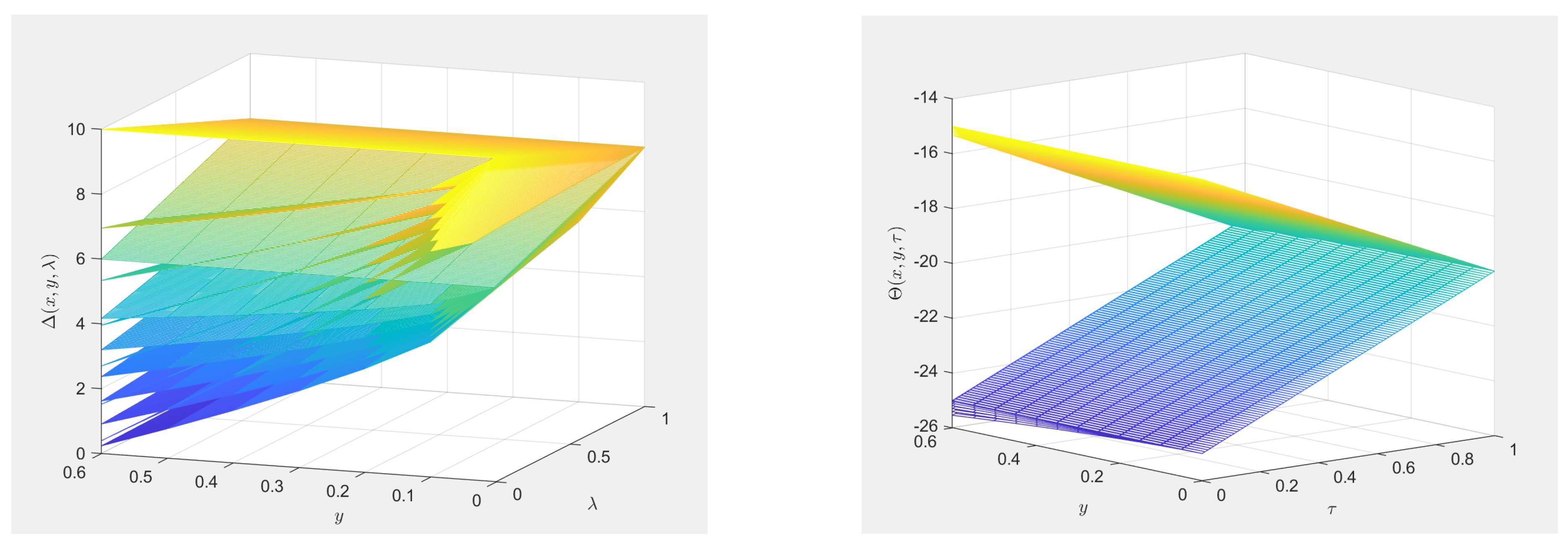
Figure 1. presents simulation results of the level sets for the fuzzy solutions in (40) and (41). The left and right subfigures show seven level sets of and at seven fixed x values, respectively. Each surface group corresponds to a or level set, with inter-surface distances characterizing the fuzzy solutions. When six y values are fixed, the variations of level sets with x and are consistent with Figure 1. The curves in the planes represent contour lines of and , respectively.
By Proposition 21 (b) of [31], the H-difference exists. Taking
its level set is:
with interval length:
Using an analogous computational approach, we obtain:
Hence, the H-difference exists.
Similarly, from (42) and (43):
Consequently:
This implies
By Proposition 21(a) of [31], the H-difference exists. Using identical methodology:
The aforementioned procedure establishes the existence of the H-difference . Heretofore, these verify the assumptions and in Theorem 2. Given that and are compact-supported and
, it follows from Theorem 2 that a -weak solution to (39) exists on and
5. U-HS Analysis
In this section, we mainly study U-HS of the solutions to the system (3). Specifically, all results presented in this section are established under the assumption of existence. We contend that U-HS idea is important for practical issues in analysis. The interesting feature of stability is that to search a U-HS of a system, who exact solution does not exist, which is typically challenging or time consuming. According to U-HS, there exists a close approximate solution of system to exact solution. As we know that mostly a mathematical models are non-linear in nature and some time its exact solution does not exist or difficult to be obtained. Therefore, we need to find best approximate solution for such problems.
Definition 10
Remark 4.
is a solution of (10) if and only if: for each and as in Definition8, there exists (depending on ) satisfying and the perturbed system
holds.
The following proof is provided only for type solutions, as the proof for type solutions follows an identical procedure and is therefore omitted.
Lemma 9.
Let be a solution of (10). Then the following inequality hold:
Proof.
By Remark 4, the system can be written as:
From Lemma 3, we obtain:
Thus:
where . Similarly:
where . □
Now we present the following two hypotheses which are helpful in building our main result:
Letting and are any solutions of (3), then there exist and such that
There exist some constants (i=1, 2) and with
Theorem 3.
Under the conditions in Theorems 1 and 2 and assumptions and , the symmetry coupled system (3) is U-HS if .
Proof.
Similarly, one can obtain
According to (45) and (46), its matrix can be expressed as the following form:
where and . Letting , then we solve the matrix inequality (47) and have
which mean that
where . Thus, the new fuzzy fractional partial differential symmetry coupled system (3) is U-HS. □
6. Conclusions
In this paper, the existence and stability of solutions for a class of C-K FFPDEs symmetry coupled systems involving gH-type difference were studied. Its form is as follows
for any and . By employing Schauder fixed point theorem (i.e., Lemma 6), the relevant results were obtained under more general situations without Lipschitz conditions, which is common and very important.
For the work of this paper, the innovation points are as follows:
- By incorporating concepts of relative compactness and utilizing Schauder fixed point theorem, the existence of two classes of gH-weak solutions for (48) was proved without Lipschitz condition. Compared with [36], the system is considered in a more general setting in this study, which enhances its practical significance.
- By constructing specific examples, the existence of two classes of gH-type weak solutions was verified. Based on the obtained two classes of weak solutions, numerical simulations were conducted for analysis. The results demonstrate that the existence of solutions to (48) was established.
- Within the theoretical framework of Ulam-Hyers stability, the stability analysis of (48) was proposed. However, investigations into the existence theory and stability analysis of solutions for symmetry coupled systems remain scarcely documented. Moreover, the stability conditions reveal the long-term evolutionary trends of species populations under fractal habitats and fuzzy environmental carrying capacity, providing guidance for endangered species conservation strategies. Thus, the symmetry coupled system (48) exhibits substantial research value.
Compared with the existing research, the type of fuzzy fractional derivative investigated in this paper is more extensive, and a new demonstration method was adopted. A series of new conclusions were obtained, and the stability proof of the symmetry coupled system was given. Although the current research focuses on the field of PDEs, the future work intends to apply the method system proposed in this paper to other mathematical structures and engineering problems, including fuzzy stochastic fractional differential equations, time-delay systems, neural networks, signal processing and other directions.
Author Contributions
Conceptualization, L.-C.J. and H.-Y.L.; Methodology, L.-C.J. and H.-Y.L.; Software, L.-C.J. and Y.-X.Y.; Validation, L.-C.J., H.-Y.L. and Y.-X.Y.; Writing��original draft preparation, L.-C.J.; Writing��review and editing, L.-C.J., H.-Y.L. and Y.-X.Y.; Visualization, L.-C.J. and Y.-X.Y.; Project administration, H.-Y.L.; Funding acquisition L.-C.J., H.-Y.L. and Y.-X.Y. All authors have read and agreed to the published version of the manuscript.
Funding
This work was supported in part by the Scientific Research and Innovation Team Program of Sichuan University of Science and Engineering (SUSE652B002) and the Opening Project of Sichuan Province University Key Laboratory of Bridge Non-destruction Detecting and Engineering Computing (2024QZJ01).
Data Availability Statement
No new data were created or analyzed in this study. Data sharing is not applicable to this article.
Conflicts of Interest
The authors declare that they have no conflict of interest.
Abbreviations
The following abbreviations are used in this manuscript:
| gH- | Generalized Hukuhara |
| C-K | Caputo–Katugampola |
| PDEs | partial differential equations |
| FPDEs | fractional partial differential equations |
| FFPDEs | fuzzy fractional partial differential equations |
| H- | Hukuhara |
| - | Hausdorff metric |
| U-HS | Ulam–Hyers stability |
| BF | Buckley–Feuring |
References
- Katugampola, U.N. New approach to a generalized fractional integral. Appl. Math. Comput. 2011, 218, 860–865. [CrossRef]
- Singh, J.; Agrawal, R.; Baleanu, D. Dynamical analysis of fractional order biological population model with carrying capacity under Caputo-Katugampola memory. Alex. Eng. J. 2024, 91, 394–402. [CrossRef]
- Singh, J.; Gupta, A.; Baleanu, D. Fractional dynamics and analysis of coupled Schrödinger-KdV equation with Caputo-Katugampola type memory. ASME. J. Comput. Nonlinear Dynam. 2023, 18, 091001. [CrossRef]
- Katugampola, U.N. Existence and uniqueness results for a class of generalized fractional differential equations. preprint, arXiv:1411.5229 2014. [CrossRef]
- Podlubny, I. Fractional Differential Equations. Mathematics in Science and Engineering; Academic Press, Inc.: San Diego CA, 1999; Volume 198.
- Kilbas, A.A.; Srivastava, H.M.; Trujillo, J.J. Theory and Applications of Fractional Differential Equations. North-Holland Mathematics Studies; Elsevier Science B.V.: Amsterdam, The Netherlands, 2006; Volume 204. [CrossRef]
- Wu, Z.B.; Min, C.; Huang, N.J. On a system of fuzzy fractional differential inclusions with projection operators. Fuzzy Sets and Systems 2018, 347, 70–88. [CrossRef]
- Zhang, Z.; Karniadakis, G. Numerical Methods for Stochastic Partial Differential Equations with White Noise. Applied Mathematical Sciences, Springer, Cham, 2017; Volume 196, pp. 161–329. [CrossRef]
- Magin, R.L. Fractional calculus models of complex dynamics in biological tissues. Comput. Math. Appl. 2010. 59, 1586–1593. [CrossRef]
- Saha, R.S. Nonlinear Differential Equations in Physics–Novel Methods for Finding Solutions. Springer, Singapore, 2020. [CrossRef]
- Lan, H.Y.; Nieto, J.J. On a system of semilinear elliptic coupled inequalities for S-contractive type involving demicontinuous operators and constant harvesting. Dyn. Syst. Appl. 2019. 28, 625–649.
- Ding, M.H.; Liu, H.; Zheng, G.H. On inverse problems for several coupled PDE systems arising in mathematical biology. J. Math. Biol. 2023, 87, 86. [CrossRef]
- Zhang, Z.; Cheng, X. Existence of positive solutions for a semilinear elliptic system. Topol. Methods Nonlinear Anal. 2011, 37, 103–116.
- Zhang, F.; Lan, H.Y.; Xu, H.Y. Generalized Hukuhara weak solutions for a class of coupled systems of fuzzy fractional order partial differential equations without Lipschitz conditions. Mathematics 2022, 10, 4033. [CrossRef]
- Muatjetjeja, B.; Mbusi, S.O.; Adem, A.R. Noether symmetries of a generalized coupled Lane-Emden-Klein-Gordon-Fock system with central symmetry. Symmetry 2020, 12, 566. [CrossRef]
- Nguyen, H.T.; Sugeno, M. Fuzzy Systems: Modeling and Control. The Handbooks of Fuzzy Sets. Springer, New York, 1998; Volume 2. [CrossRef]
- Chaki, J. A fuzzy logic-Based approach to handle uncertainty in artificial intelligence. In: Handling Uncertainty in Artificial Intelligence, SpringerBriefs in Applied Sciences and Technology. Springer, Singapore, 2023, pp. 47–69. [CrossRef]
- Osman, M. On the fuzzy solution of linear-nonlinear partial differential equations. Mathematics 2022, 10, 2295. [CrossRef]
- Pandey, P.; Singh, J. An efficient computational approach for nonlinear variable order fuzzy fractional partial differential equations. Comput. Appl. Math. 2022, 41, 38. [CrossRef]
- Mazandarani, M.; Kamyad, A.V. Modified fractional Euler method for solving fuzzy fractional initial value problem. Commun. Nonlinear Sci. Numer. Simul. 2013, 18, 12–21. [CrossRef]
- Singh, P. A fuzzy fractional power series approximation and Taylor expansion for solving fuzzy fractional differential equation. Decis. Anal. J. 2024, 10, 100402. [CrossRef]
- Akram, M.; Yousuf, M.; Allahviranloo, T. An analytical study of Pythagorean fuzzy fractional wave equation using multivariate Pythagorean fuzzy Fourier transform under generalized Hukuhara Caputo fractional differentiability. Granul. Comput. 2024, 9, 15. [CrossRef]
- Baleanu, D.; Wu, G.C.; Zeng, S.D. Chaos analysis and asymptotic stability of generalized Caputo fractional differential equations. Chaos Solitons Fractals 2017, 102, 99–105. [CrossRef]
- Van, H.N.; Vu, H.; Duc, T.M. Fuzzy fractional differential equations under Caputo-Katugampola fractional derivative approach. Fuzzy Sets and Systems 2019, 375, 70–99. [CrossRef]
- Wang, B.; Li, X. Modeling and dynamical analysis of a fractional-order predator-prey system with anti-predator behavior and a holling type IV functional response. Fractal. Fract. 2023, 7, 722. [CrossRef]
- Ali, A.; Bibi, F.; Ali, Z. Investigation of existence and Ulam’s type stability for coupled fractal fractional differential equations. Eur. J. Pure. Appl. Math. 2025, 18, 5963–5963. [CrossRef]
- András, S.; Mészáros, A.R. Ulam-Hyers stability of elliptic partial differential equations in Sobolev spaces. Appl. Math. Comput. 2014, 229, 131–138. [CrossRef]
- Son, N.T.K. Uncertain fractional evolution equations with non-Lipschitz conditions using the condensing mapping approach. Acta. Math. Vietnam. 2021, 46, 795–820. [CrossRef]
- Long, H.V.; Son, N.T.K.; Tam, H.T.T. The solvability of fuzzy fractional partial differential equations under Caputo gH-differentiability. Fuzzy Sets and Systems 2017, 309, 35–63. [CrossRef]
- Román-Flores, H.; Rojas-Medar, M. Embedding of level-continuous fuzzy sets on Banach spaces. Inform. Sci. 2002, 144, 227–247. [CrossRef]
- Stefanini, L. A generalization of Hukuhara difference and division for interval and fuzzy arithmetic. Fuzzy Sets and Systems 2010, 161, 1564–1584. [CrossRef]
- Lakshmikantham, V.; Mohapatra, R.N. Theory of Fuzzy Differential Equations and Inclusions. Taylor and Francis Group 2003. [CrossRef]
- Worth, R.E. Boundaries of semilinear spaces and semialgebras. Trans. Amer. Math. Soc. 1970, 148, 99–119. [CrossRef]
- Stefanini, L.; Bede, B. Generalized Hukuhara differentiability of interval-valued functions and interval differential equations. Nonlinear Anal. 2009, 71, 1311–1328. [CrossRef]
- Bede, B. Mathematics of Fuzzy Sets and Fuzzy Logic. In Studies in fuzziness and soft computing. Springer Berlin, Heidelberg, 2013. [CrossRef]
- Rashid, S.; Jarad, F.; Alamri, H. New insights for the fuzzy fractional partial differential equations pertaining to Katugampola generalized Hukuhara differentiability in the frame of Caputo operator and fixed point technique. Ain. Shams. Eng. J. 2024, 15, 102782. [CrossRef]
- Zhang, F.; Xu, H.Y.; Lan, H.Y. Initial value problems of fuzzy fractional coupled partial differential equations with Caputo gH-type derivatives. Fractal. Fract. 2022, 6, 132. [CrossRef]
- Agarwal, R.P.; Arshad, S.; O’Regan, D.; Lupulescu, V. A Schauder fixed point theorem in semilinear spaces and applications. Fixed Point Theory Appl. 2013, 2013, 306. [CrossRef]
- Long, H.V.; Son, N.T.K.; Ha, N.T.M.; Son, L.H. The existence and uniqueness of fuzzy solutions for hyperbolic partial differential equations. Fuzzy Optim. Decis. Mak. 2014, 13, 435–462. [CrossRef]
Figure 1.
Numerical simulation for fuzzy solutions of (39)
Disclaimer/Publisher’s Note: The statements, opinions and data contained in all publications are solely those of the individual author(s) and contributor(s) and not of MDPI and/or the editor(s). MDPI and/or the editor(s) disclaim responsibility for any injury to people or property resulting from any ideas, methods, instructions or products referred to in the content. |
© 2025 by the authors. Licensee MDPI, Basel, Switzerland. This article is an open access article distributed under the terms and conditions of the Creative Commons Attribution (CC BY) license (http://creativecommons.org/licenses/by/4.0/).
Copyright: This open access article is published under a Creative Commons CC BY 4.0 license, which permit the free download, distribution, and reuse, provided that the author and preprint are cited in any reuse.


