
Submitted:
12 September 2025
Posted:
12 September 2025
You are already at the latest version
Abstract
While the established theory of computer-aided geometric design (CAGD) suggests that rational Bernstein--B\'ezier polynomials associated with control points can be used to accurately represent conics and quadrics, this paper shows that the same goal can be achieved in a different manner. More specifically, rational Lagrange polynomials of the same degree, associated with nodal points lying on the true curve or surface, can be combined with appropriate weights to yield equivalent numerical results. Although this replacement may not be crucial for CAGD purposes, it proves useful for the direct implementation of boundary conditions in isogeometric analysis, since it allows the use of nodal values on the exact boundary.
Keywords:
Lagrange polynomial
; Bernstein-Bézier polynomial
; computer-aided geometric design
; isogeometric analysis
; finite element method
MSC: 41A10; 41A15; 65N30
1. Introduction
Since the mid-1970s, research in computer-aided geometric design (CAGD) has heavily relied on Bernstein-Bézier polynomials as a foundational tool for representing and manipulating curves and surfaces. This preference stems primarily from their strong geometric intuition: the shape of a Bézier curve or surface is governed by a finite set of control points, which usually lie outside the geometric entity itself and act as handles for interactive design and editing. A second important reason is the mathematical flexibility of the Bernstein basis, which supports essential operations such as degree elevation, subdivision, and knot insertion, enabling local refinement without altering the global geometry’s key features for adaptive modeling and analysis [1].
Furthermore, Bernstein polynomials are central to the construction of non-uniform rational B-splines (NURBS), which extend polynomial representations by incorporating weights. This allows for the exact representation of conic sections and other analytic shapes, a capability critical to engineering design and manufacturing applications. As a result, Bernstein-based representations remain a cornerstone of modern CAD/CAM systems and form the basis of isogeometric analysis, which unifies geometric modeling ([1,2,3]) and finite element analysis ([4]).
It is well established in the literature that the weighted, or rational, Bernstein-Bézier formulation enables the exact representation of conic sections and quadrics, provided that suitable weights are assigned to the appropriate control points (e.g., see [1,2,3], among hundreds of other sources). This capability is one of the key advantages of rational Bézier and NURBS representations in computer-aided geometric design and CAD systems. However, there have also been a limited number of investigations into using Lagrange polynomials for similar geometric modeling tasks, particularly for approximating circular arcs and ellipses, but for efficient analysis as well [5,6]. Focusing on circular arcs, these approaches can produce visually acceptable results but typically suffer from small but non-negligible numerical errors due to the inability of polynomial Lagrange interpolation to exactly represent circular shapes [7,8,9,10].
On the other hand, Lagrange interpolation in itself is quite robust and efficient. The mentioned instabilities are related to Runge oscillations, which only occur on equidistant nodal distributions (for example, see Ref. [11]). Within this context, Lagrange interpolation might break down in such a case for high polynomial orders. However, a simple remedy is to use non-equidistant nodal distributions that accumulate nodes near the interval boundaries. This has been done in the Spectral Element Method (SEM), where Gauss-Lobatto-Legendre (GLL) or Gauss-Lobatto-Chebyshev (GLC) nodes are employed to replace equidistant nodes [12,13]. Such non-equidistant nodes result in excellent interpolation properties and mitigate any instabilities. Employing GLL or GLC nodes, it has been noticed that the element matrices are well conditioned and not numerical problems arise [14].
From the above discussion, it follows that Lagrange polynomials offer high accuracy when applied in conjunction with non-equidistant nodal distributions (e.g., GLL or GLC points), whereas Bernstein polynomials possess the advantage of incorporating weights that enable the exact representation of conics and quadrics.
In this paper, we lay the groundwork for combining these two advantages into a unified framework. Specifically, we determine the weights that can be directly applied to both uniform and non-uniform Lagrange polynomials, thereby constructing an equivalent functional basis of rational Lagrange polynomials.
2. General Formulation
2.1. Degree Elevation Using Bernstein-Bézier Polynomials
Rational Bézier curves can be readily handled within the framework of computer-aided geometric design (CAGD). Beginning with a low degree, such as , and employing an appropriate set of homogeneous (projected) control points , with weights (), the shape of the curve remains invariant under degree elevation, with the control points being updated accordingly at each step as follows:
with
The updated homogeneous weights that accompany the elevated control points (or the 2-D analogue) follow exactly the same convex-combination pattern as for the degree elevation formula for Bernstein (polynomial) Bézier curves (cf. Eq. (1)):
with the boundary values preserved,
Once the homogeneous points are updated, we obtain the Cartesian control points simply by dehomogenising:
This degree-elevation step may be applied repeatedly; after k successive elevations (to degree ) the same recurrence is used at each stage, guaranteeing that the rational Bézier curve’s shape remains unchanged while its control-polygon flexibility increases.
2.2. Replacing Bernstein Polynomials by Lagrange Polynomials
While the procedure of degree elevation is straightforward in conjunction with Bernstein polynomials, it is not the case with Lagrange polynomials. Of course, since both sets span the same space (of powers ), these two sets are linearly interrelated.
In more detail, let us consider the reference unit length . For a certain degree n, i.e., for the nodal points , let be the row vector including all relevant univariate Lagrange polynomials of degree n:
and be the row vector including all univariate Bernstein polynomials of degree n:
Then, we can write:
where (from Bernstein to Lagrange) and (from Lagrange to Bernstein) are transformation matrices, which have been discussed in detail elsewhere [15]. For the purposes of this paper, the determination of transformation matrix that must be applied to Lagrange polynomials–according to Eq. (9)–plays a critical role.
Actually, since a linear transformation occurs between two functional sets (here the subscripts denote, B: Bernstein-Bézier, L: Lagrange), not only the different sets of polynomials (cf. Eq. (8) and Eq. (9)), but also the homogeneous coordinates () and the weights () are interrelated according to the following theorem.
Theorem
The homogeneous (projected) cordinates of nodal points () associated with the true boundary of a curve in the Lagrange formulation, are related with the projected control points () of the same curve in the Bernstein formulation, as follows:
Moreover, the weights in the Lagrange formulation are related with the weights in the initial Bernstein formulation, as follows:
In more detail, to obtain the nodal points on the true curve, it is necessary to divide the vector of homogeneous coordinates (calculated using Eq. (10)) by the vector of associated weights (estimated by Eq. (11)).
Proof.
The proof is based on the fact that the shape of the curve under consideration is preseved (in shape and parametrically [2]). Therefore, expressing first in terms of Lagrange polynomials (forming the vector ) and second in terms of Bernstein polynomials (forming the vector ), we have:
Substituting through Eq. (9) into the utmost right term of Eq. (12), we receive:
Remark-1: Weights. In a previous work (see, [15], pp. 80–83])) regarding a circular arc of 90 degrees modeled by quadratic Bernstein polynomials, Eq. (11) has been proven from scratch (after manipulation), but here the formula was generalized in matrix form.
Therefore, if we restrict our study, for example, to a circular arc with a central angle of , we may begin with a quadratic polynomial () associated with the weights (see, Ref. [16]). Subsequently, Eq. (3) can be applied to compute the weights resulting from successive degree elevations until a certain degree .
For each of the abovementioned degree elevations, we can determine the transformation matrix , and then implement Eq. (11) to determine the weights associated with the rational Lagrange polynomials.
Remark-2: Nodal points. By definition, non-uniform rational B-splines (NURBS) is a non-uniform interpolation. This means that even if the interval is uniformly subdivided by the points , the corresponding nodal points do not generally subdivide the curve in equal arc lengths. This issue is shown later in Section 3.1.2.
2.3. Determination of Transformation Matrix
In this section, we present two alternative procedures for constructing the transformation matrix.
2.3.1. Detailed Algebraic Procedure
Since Bernstein and Lagrange polynomials span the same space (of monomials ), any univariate function will be equally written in any of them. By equating the coefficients of the same powers , we can derive a relationship between nodal values and generalized coefficients . This relationship is set in the form:
Example: Let we set the function in terms of Lagrange polynomials polynomials (based on uniform nodal points at ), as follows:
Alternatively, let us we set the same function in terms of Bernstein polynomials:
By equating the coefficients of the same powers between the quadratic polynomials given by Eq. (15) and Eq. (16), we receive the following system:
Equivalently, Eq. (17) can be written as follows:
Equation (18) can be solved for either of the two vectors. Choosing the second one, after matrix inversion we have:
Comparing Eq. (20) with the first equality of Eq. (15), the unique representation –in terms of ()– leads to the relationships:
In matrix form, Eq. (21) is rewritten as:
By inverting Eq. (22), we receive:
Therefore, if we pack all triplets into the following relevant column vectors:
the above relationships are written in matrix form as follows:
and
with
2.3.2. A Shorter Numerical Procedure
Since the transformation matrices merely relate the nodal vector with the coefficients vector , in a unique way (because of the same polynomial degree), we can start by implementing the well known formula:
at the uniform points (with which the nodal values are associated), and thus we shortly receive:
Therefore, by applying the Bernstein-based series expansion Eq. (28) at three uniform parameters , we can shortly obtain the transpose of the transformation matrix , which denotes the change from Lagrange (L) to Bernstein (B) basis.
2.4. From Approximation Theory and Numerical Analysis to CAGD
The conclusions of Section 2.3 pertain to the relationship between the nodal values and the generalized coefficients . Within the context of computer-aided geometric design (CAGD), the nodal values correspond to the Cartesian coordinates , whereas the generalized coefficients are interpreted as the control points .
In this context, in non-rational formulation, the substitute of Eq. (28) is
Therefore, when the weights equal unity (), we can apply Eq. (30) at the nodal points on the true curve (at specific–so far uniform–parameters ) and then solve in . The matrix which relates the vectors and is the transformation matrix under demand, i.e., .
In the general case of non-unity weights (), Eq. (30) converts to:
where the projected (homogeneous) control points are given by the well-known formula:
Depending on the value of parameter , the row vector in the numerator of Eq. (31) is one out of the three rows of the matrix involved in Eq. (28). In more detail, considering Eq. (32), we have:
The totality of Eqs. (33) to (35) makes the column vector of nodal points on the curve, at the uniform values of parameter , and thus we can write:
where
Below we shall see how the nodal coordinates are introduced into the formulation. Actually, we return to Eq. (31) and substitute the row vector of Bernstein polynomials by the row vector of Lagrange polynomials using the second equality of Eq. (25). Furthermore, by virtue of Eq. (36), we have:
Regarding Eq. (38), one may observe that the weight in the numerator is incorporated into the projected (homogeneous) coordinate of the i-th control point , whereas in the denominator appears as a factor of the Bernstein polynomial associated with current control point.
It is worth-mentioning that although the three nodal points () subdivide the circular arc into two equal parts, due to the weights , in general, even if each part is further subdivided into uniform increments the mapping from the prameter space to the natural space is non-uniform. This means that the increments of the corresponding central angles will be non-uniform, as wll be later discussed in Section 3.1.2.
The determination of the transformation matrix, , is discussed in Section 3.
3. Weights
3.1. Circular Arc with Central Angle
3.1.1. Uniform Distribution
We consider a circular arc of central angle and radius , in the first quadrant. We start with degree in conjunction with the well-known control points , , and , and the initial weights (, according to [16]).
As a first step, we continuously elevate the polynomial degree applying Eq. (3), thus determining the updated weights for each degree. Furthermore, applying Eq. (1), we determine the Lagrange-based weights.
The second step is to determine the transpose of the transformation matrix , for the desired degree p. Collectively, for degrees until , we have:
Regarding the associated weights, these are shown in Table 1.
3.1.2. Non-Uniform Distribution
Now, we consider the case of non-uniform distribution of nodal points along the edges of a 27-node classical transfinite element (shown in Figure 1), where the nodes along the horizontal edge AB are located at the non-uniform positions:
The formulation is the same, with the only difference regarding the , which now becomes:
whence the updated weight vector (according to Eq. (11)) becomes:
One may obseve in Eq. (46), that the non-uniform node distribution (Eq. (44)) leads to the non-symmetric form of vector .
In the following, we shall demonstrate that both a straight segment and a circular arc can be represented accurately.
I. Straight segment
Taking the uniform set of control points associated with the Bernstein basis of degree (considering weights ):
and left-multiplying by the non-uniform transformation matrix given by in Eq.(45) according to Eq. (10), we derive the true non-uniform coordinates:
The result of Eq. (48) is validated by the non-uniform nodal points shown on the edge AB of Figure 1.
Remark: In contrast, if the uniform set of Eq. (47) had been multiplied by the uniform matrix of Eq. (42), the location of the nodal points on the straight segment would be uniform as well.
II. Circular Arc
Concerning the projected coordinates in Lagrange formulation, they can be calculated through Eq. (10), using the Cartesian coordinates of control points in Bernstein formulation (Table 2) in combination with the associated weights shown in Table 1. Afterwards, the projected coordinates in Lagrange formulation are divided by the corresponding entries of vector given by Eq. (46).
The results of the above procedure is illustrated in Figure 2, where the nodal sequence {1,2,3,4,5,6} of Lagrangian formulation is in the counter-clockwise direction. The five central angles formed by the radii associated with the ends of each nodal segment (i.e., 1-2,…,5-6), are shown in Table 2. One may observe that nodal point 4 (at ) is exactly in the middle of the circular arc (i.e., ). However, the other nodes do not accurately split the two parts in three (nodes 1 to 4) and two (nodes 4 to 6) segments, respectively, of equal magnitude. In other words, the increments of the parameter differ from the increments of central angle of Lagrangian formulation, as also happens with the identical central angle in the Bernstein formulation (with control points to illustrated in magenta color).
Finally, the rational and non-rational shape functions associated with the nodal points 1-to-6 on the circular arc are shown in Figure 3, where the same color has been used for corresponding curves.
3.2. Central Angle Different than
The control triangle of the arc must be isosceles, the end weights can be set to 1, and the middle weight is the cosine of the angle between the chord joining the endpoints and one of the legs [16].
Therefore, if the central angle of the circular arc equals to , to accurately represent the geometry, one choice of the weights is:
However, the end weights do not have to remain 1; the arc can be "reweighted" using the shape invariace ratio:
For example, an equivalence choice to that of Eq. (49) may be:
4. Examples
4.1. Example-1: The Case of Degree p=2
Let us consider a circular arc in the first quadrant, with a central angle of . Considering the transformation matrix given by Eq. (39) as well as the well-known vector of weights (Ref. [16]), the Lagrangian weights are given by the vector (see Eq. (11)):
Moreover, Eq. (10) depicts that the nodal points on the circular arc are given as:
To obtain the Cartesian coordinates of the nodal points onto the circular arc, the entries of matrix (Eq. (53)) must be divided by the corresponding elements of vector (Eq. (52)), thus obtaining:
Therefore, in Eq. (54) we eventually derived the two endpoints plus the middle point of the circular arc.
Remark: In the above case where , the nodal points on which the equivalent rational Lagrange polynomials are based, have divided the circular arc in two equal parts, i.e., and .
Nevertheless, for higher degrees (i.e., ) the nodal points are not uniformly distributed. Since the parameterization does not change with degree elevation [2], the findings of this section for are sufficient to determine the position of the nodal points for higher degrees.
Within this context, for any polynomial degree which is related to parameter values , the nodal points are calculated through the quadratic model of this subsection as follows:
4.2. Example-2: The Case of Degree p=3
4.2.1. Straight Line
First, it is worthy to comment on the representation of a straight line through rational interpolation. Within this context, let us consider a segment AB, made of points A(0,0) and B(1,1), which is uniformly subdivided in three equal parts by points C and D, as shown in Figure 4. Assuming that the parametric space along AB corresponds to the interval , it is reasonable to consider that points C and D correspond to and , respectively. Therefore, the associated Lagrange polynomials are given by:
Given the weights
associated with the points (A, C, D, B), the rational approximation is given as:
and
By definition, due to the cardinality of rational shape functions, the parameters correspond to the points A, C, D, and B, respectively. In all cases, it was found that the whole mapping is the straight segment AB itself. For example, if the segment lies on the bisector of the right angle in the first quadrant, the nodal points are equal each other, and thus the same rational basis functions lead to the same output ().
Moreover:
- When , the mapping is uniform, i.e., .
- In contrast, when , the mapping is non-uniform.
4.2.2. Circular Arc of
Now, we focus on the representation of the circular arc, using rational Lagrange polynomials of degree .
While Eq. (56) is still valid, in current case–due to symmetry with respect to the bisector of first quadrant–the weights are taken as
The question is whether it is possible to determine a unique value of the weight such that the corresponding rational Lagrange polynomials, based on the uniform nodes (A, C, D, B) in the physical space, can exactly represent the circular arc. In this regard, by means of a counterexample, we will show that this is not generally possible.
Actually, substituting Eq. (58) and Eq. (59) into the desired identity:
we derive a polynomial of sixth degree in , as follows:
with
One may observe that the constant term a priori vanishes (Eq. (63)), while the root of Eq. (64) provides the value . Moreover, the closest root of the binomial given by Eq. (65) is slightly different as it equals to , whereas Eq. (66) vanishes at a higher value . Furthermore, Eq. (67) has two complex roots, and the rest two equations substantially differ from . As a result, there is no real value which makes all the coefficients to be zero.
In conclusion:
- It is not generally possible to accurately represent a circular arc using equi-distant nodal points, even if rational Lagrange polynomials are used. Based on optimization techniques, where an objective function such as becomes minimum, it is possible to determine a value which compromizes the conditions . Nevertheless, small deviations from the ideal circle will be noticed (e.g., after the fourth decimal point).
4.3. Example-3: The Case of Degree p=5
Let us deal with the uniform case of . For , the Lagrange polynomials are as follows:
The Cartesian coordinates of control points in the Bernstein model are as follows:
The circular arc in the first quadrant is subdivided at the nodal points which correspond to the parametric vector . To determine them, it becomes necessary to apply the rational Bézier formula:
where the coordinates are given by Eq. (71), while the corresponding weights are isolated in the following row vector:
Based on the Cartesian coordinates of nodal points on the true circular arc according to Eq. (72), and using the weights shown in Table 1, repeated below:
the parametric equation of the circular arc is as follows:
The interesting issue is the position of the nodal points in the Lagrangian model. While for quadratic interpolation (i.e., ) the nodal points are the two endpoints and the middle point, in all other situations they are arranged in a non-uniform way. For example, for current case where , the polar angle for the nodal points (1 to 6 in counter-clockwise direction) in the first quadrant is shown in Table 4. One may observe that, although is a constant, the corresponding central angles differ one another.
5. Spherical Cap
The above formulation is applicable to surfaces as well. As an example, we consider a spherical cap, which is exactly one-sixth of a unit sphere’s surface. It is known that the quadratic interpolation is not capable of accurately representing this curvilinear surface [17]. In contrast, quartic interpolation () in conjunction with 25 control points can accurately represent this cap [18] (see, the parametric space in Figure 5).
Regarding the southern spherical cap, the location of 25 control points and the associated weights are available through the MATLAB function southcap=rsmak(‘southcap’). With respect to Bernstein polynomials of degree , the Cartesian coordinates and the associated weights of control points are shown in Table 5. There, one may observe that the analytical formula is not an ideal tensor product, in the sense that the weights associated with the internal control points are not products of the corresponding boundary ones (i.e., ).
By analogy to the one-dimensional procedure reported in the previous sections of this paper, the algorithm to derive the nodal points (on the true sperical surface) and the associated weights is as follows:
- Calculate the projected control points and the associated weights . This is implemented using the abovementioned built-in MATLAB function southcap=rsmak(‘southcap’).
- Create the total transformation matrix , of size (see below). In more detail, if the one-dimensional matrix of Eq. (41) is shortly written as:the 2D analog–applied to a surface patch–becomes:
- Multiply the control points by the abovementioned , and thus determine the projected nodal points :
- Multiply the weights vector by the abovementioned , and thus derive the weights associated with Lagrange polynomials:
The implementation of the above algorithm to the southern spherical cap of a sphere of unit radius () gives the numerical values shown in Table 6. Based on these data, for every pair the image was found to belong to the true spherical cap (numerical error less than ), and also coincided with the corresponding point obtained using rational Bernstein plynomials.
6. A Boundary-Value Problem
In this section we study the numerical solution in the quarter of an annulus, with internal radius and external radius . The corresponding temperatures on the circular edges are and , whereas the flux perpendicular to the straight edges vanish (), as shown in Figure 6.
In terms of the radius r (with ), the analytcal solution is given by:
Numerical results are presented in terms of the error norm in percent, which is defined as follows:
Each of the two circular arcs was divided into two equal parts using 3 nodes on the true boundary, whereas the weights associated with quadratic Lagrange polynomials were . The number of uniform sudivisions in the radial direction varied among 1 and 25 (i.e., degree ), and relevant Lagrange polynomials were combined with unit weights. For any given value , the total number of nodes in the model, on the true boundary and the interior, is .
The calculated error norm (in percent) is shown in Figure 7. It may be observed that up to the convergence is monotonic, after which it (not shown) increases slightly. It is also worth noting that even for the coarsest model (i.e., ), the exact analytical value of the area
was accurately approximated by numerical performing the integral of the determinant of Jacobian matrix, i.e.,
7. Discussion
It was shown that the set of weights associated with Bernstein polynomials and control points, which determine a certain curve , can be successfully replaced by another set of weights associated with Lagrange polynomials of the same degree and nodal points on the same true curve.
The key point is to determine the transformation matrix, , which relates the vector of Bernstein polynomials (B) with that of Lagrange polynomials (L). This relationship depends on the parametric location of the nodal points, thus enabling uniform and non-uniform nodal positions.
Starting with the consituents of the Bernstein-Bézier curve, i.e., the control points and the weights , we can easily determine the projected nodal points and their weights in the Lagrangian formulation, and eventually find the nodal points on the true curve . Based on them, for any arbitrary parameter we can calculate the associated rational Lagrange polynomials and then apply series expansion to determine the corresponding point . It was found that the relevant approximation accurately represents a circular arc (maximum error less than ).
The same concept is applicable to a surface (curvilinear patch) as well. As an example, we considered the spherical cap which refers to one-sixth of a sphere. It is well known that this is accurately represented by a rational Bézier surface of degree , which is not an ideal tensor product. The latter means that the weights of the interior satisfy the inequality ; therefore, since five control points exist in each direction, the denominator of the normalization will be a sum of 25 terms. A generic expression was presented to construct the total transformation matrix (of size ) in terms of the one-dimensional transformation matrix (of size ) along any edge of the quadrilateral patch. Next, the twenty-five nodal points on the true surface were determined, and for each parametric pair the spherical cap was accurately represented (maximum deviation less than ).
An additional advantage of using nodal points on the true boundary of the domain, is the fact that stiffness and mass matrices directly refer to the nodal values, , and thus boundary conditions are easily imposed. Relevant numerical results–using rational Lagrange polynomials–were presented in Section 6, where excellent convergence was reported. In addition, it is worthy to mention that identical numerical results were found when rational Bernstein-Bézier polynomials were implemented.
8. Conclusions
The usual representation of smooth patches through tensor-product rational Bernstein-Bézier polynomials, can be equivalently substituted by rational Lagrange polynomials. To maintain this numerical equivalency, it is necessary to implement transformation matrices associated with the two mutually perpendicular body-fitted directions, and thus to determine nodal points on the true boundary and corresponding weights. The geometrical concept was applied to a circular arc and a spherical cap, whereas a boundary-value problem was successfully solved for the quarter of an annulus.
Funding
This research received no external funding.
Data Availability Statement
Available upon request.
Conflicts of Interest
The authors declare no conflicts of interest.
References
- Farin, G. Curves and Surfaces for CAGD: A Practical Guide, 5th ed. Morgan Kaufmann: San Francisco, USA, 2002.
- Piegl, L; Tiller, W. The NURBS Book, 2nd ed.; Springer: Berlin, Germany, 1997.
- Hoschek, J.; Lasser, D. Fundamentals of computer aided geometric design, 2nd ed. A.K. Peters: Wellesley, Mass, 1996.
- Hughes, T. J. R.; Cottrell, J. A.; Bazilevs, Y. (2005). Isogeometric analysis: CAD, finite elements, NURBS, exact geometry and mesh refinement. Computer Methods in Applied Mechanics and Engineering 2005;194(39–41), 4135–4195.
- Schillinger, D.; Ruthala, P. K.; Nguyen, L. H. Lagrange extraction and projection for NURBS basis functions: A direct link between isogeometric and standard nodal finite element formulations. International Journal for Numerical Methods in Engineering 2016;108(6), 515–534. [CrossRef]
- Liu, B.; Xing, Y.; Wang, Z.; Lu, X.; Sun, H. Non-uniform rational Lagrange functions and its applications to isogeometric analysis of in-plane and flexural vibration of thin plates. Computer Methods in Applied Mechanics and Engineering 2017; 321, 173–208. [CrossRef]
- Lu, L. Z. Adaptive Polynomial Approximation to Circular Arcs. Applied Mechanics and Materials 2011; 50, 678–682. [CrossRef]
- Vavpetič, A. Optimal parametric interpolants of circular arcs. Computer Aided Geometric Design 2020; 80, 101891. [CrossRef]
- Vavpetič, A.; Žagar, E. A general framework for the optimal approximation of circular arcs by parametric polynomial curves. Journal of Computational and Applied Mathematics 2019; 345, 146–158. [CrossRef]
- Vavpetič, A.; Žagar, E. On optimal polynomial geometric interpolation of circular arcs according to the Hausdorff distance. Journal of Computational and Applied Mathematics 2021; 392, 113491. [CrossRef]
- De Boor, C. A Practical Guide to Splines, rev ed. Applied mathematical sciences. Springer: New York, 2001.
- Patera, A.T. A spectral element method for fluid dynamics: Laminar flow in a channel expansion. Journal of Computational Physics 1984; 54(3), 468–488.
- Pozrikidis, C. Introduction to Finite and Spectral Element Methods Using MATLAB, 2nd ed. CRC Press: Boca-Raton, 2014.
- Eisenträger, S.; Eisenträger, J.; Gravenkamp, H.; Provatidis, C.G. High order transition elements: The xNy-element concept-part II: Dynamics. Computer Methods in Applied Mechanics and Engineering 2021, 387 (Dec. 2021), 114145. [CrossRef]
- Provatidis, C.G. Precursors of Isogeometric Analysis: Finite Elements, Boundary Elements, and Collocation Methods. Solid Mechanics and Its Applications. Springer International Publishing: Cham, 2019. [CrossRef]
- Piegl, L.; Tiller, W. A menagerie of rational B-spline circles. IEEE Computer Graphics and Applications 1989; 9(5), 48–56. [CrossRef]
- Provatidis C. How accurately can spherical caps be represented by rational quadratic polynomials? WSEAS Transactions on Computers, Vol. 20, pp. 139-146, 2021, DOI: 10.37394/23201.2021.20.17, (https://wseas.com/journals/articles.php?id=273).
- Cobb, J.E. Tiling the Sphere with Rational Bézier Patches, TR UUCS-88-009, 1988. Download from: https://core.ac.uk/download/pdf/276277507.pdf (see also, Letter to the editor, Computer Aided Geometric Design 6, Issue 1, 1989).
Figure 1.
Twenty-seven node classical transfinite element.
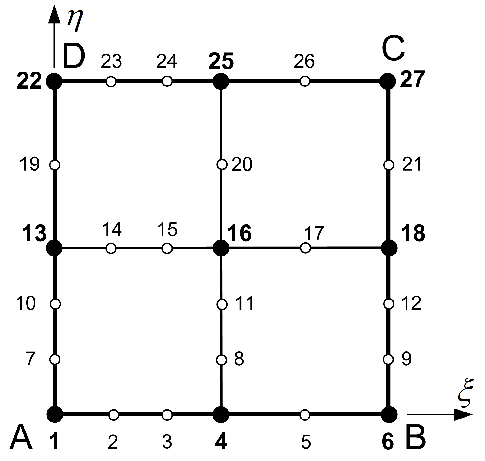
Figure 2.
Modelling of the edge AB in the 27-node classical transfinite element (see, Figure 1).
Figure 2.
Modelling of the edge AB in the 27-node classical transfinite element (see, Figure 1).
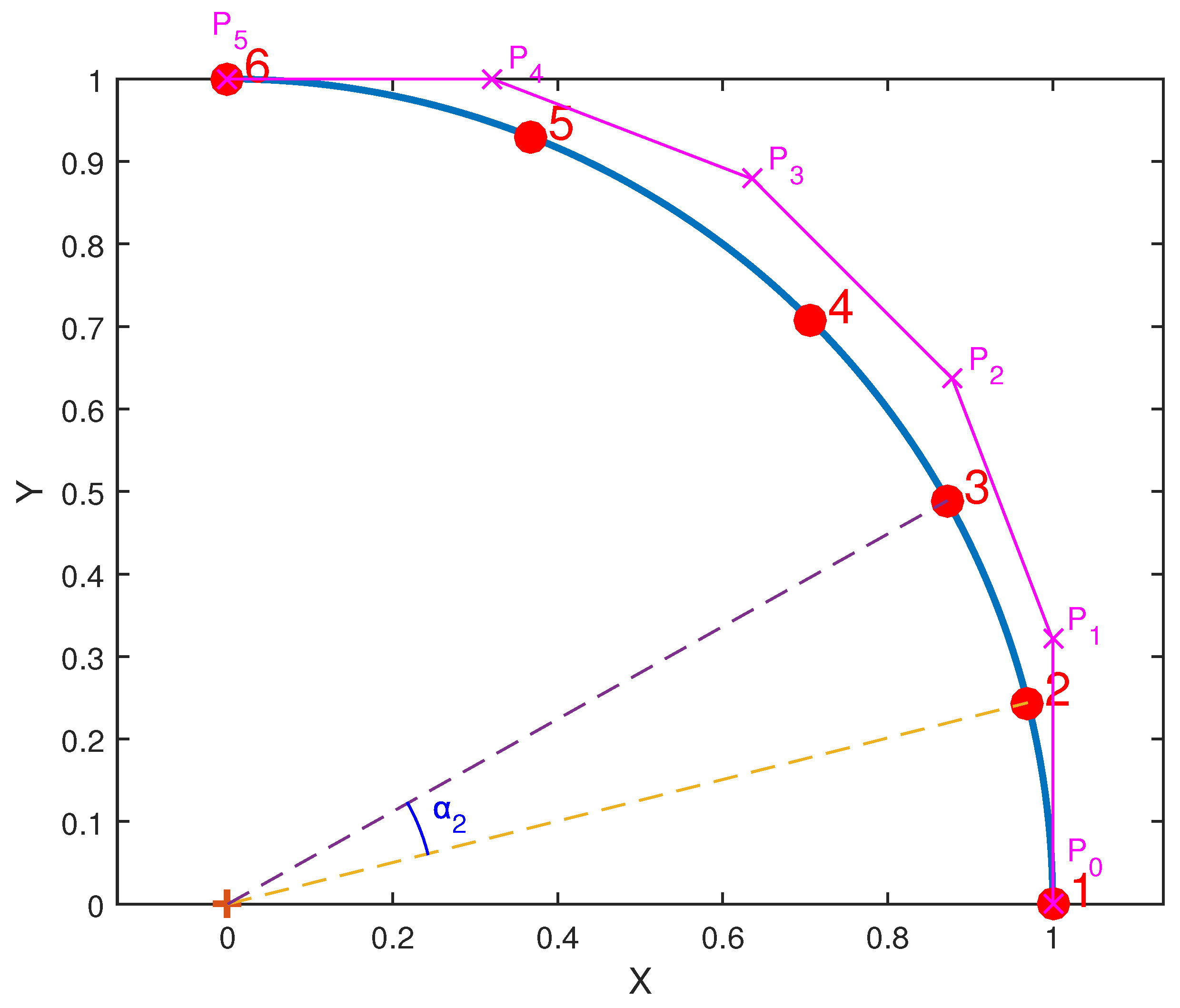
Figure 3.
Shape functions for rational (solid lines) and usual non-rational (dashed lines) Lagrange polynomials (see, nodal points on the edge AB in Figure 1).
Figure 3.
Shape functions for rational (solid lines) and usual non-rational (dashed lines) Lagrange polynomials (see, nodal points on the edge AB in Figure 1).
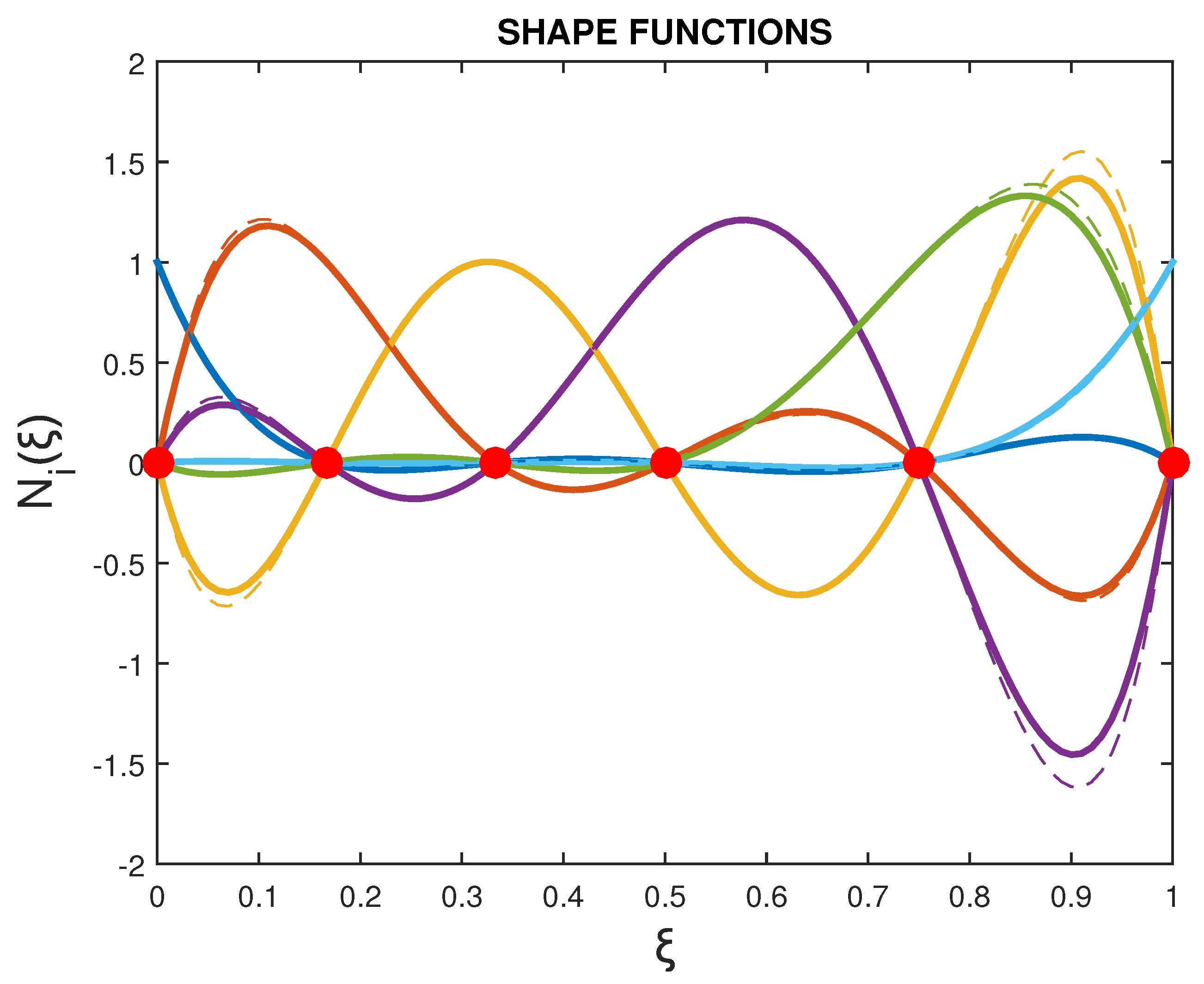
Figure 4.
Uniform subdivision of straight segment.
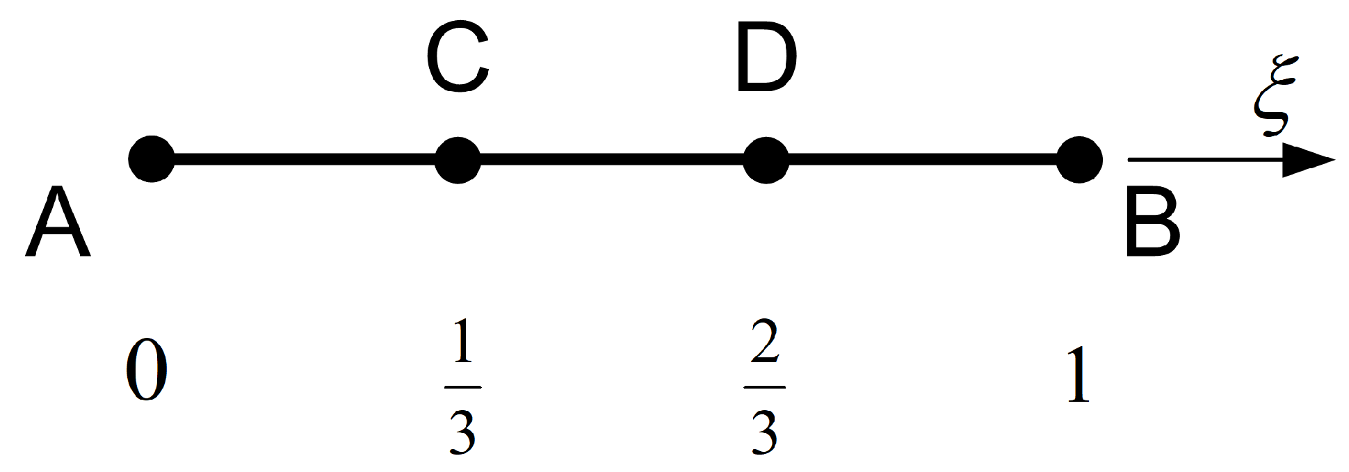
Figure 5.
Numbering of control points in the reference square ABCD.

Figure 6.
Discretization of the quarter-annulus () using: (a) Weighted (rational) Lagrange polynomials. (b) Rational Bernstein-Bézier polynomials.
Figure 6.
Discretization of the quarter-annulus () using: (a) Weighted (rational) Lagrange polynomials. (b) Rational Bernstein-Bézier polynomials.
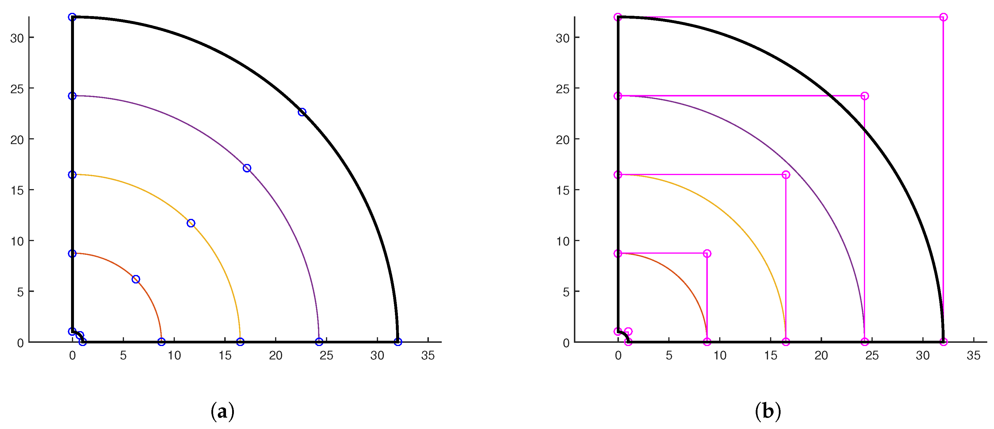
Figure 7.
Convergence quality for the quarter of annulus.
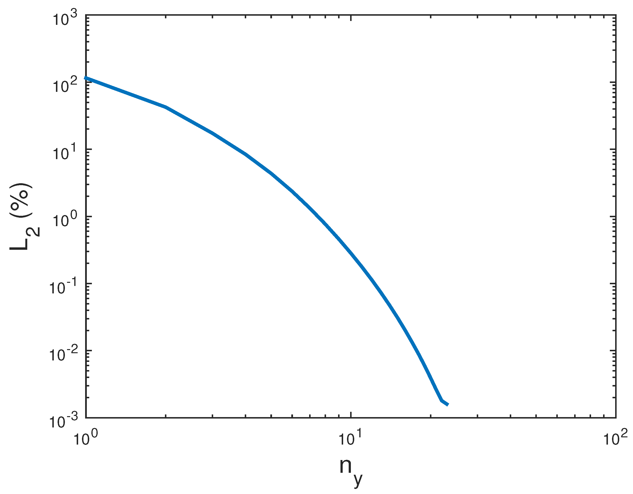

Table 1.
Weights and for the quarter of a circle.
| Degree (p) | Bernstein (Eq. (3)) | Lagrange (Eq. (11)) |
|---|---|---|
| 2 | ||
| 3 | ||
| 4 | ||
| 5 | ||
| 6 |
Table 2.
Central angles and , with (in degrees) associated with the endpoints of .
| 0 | 1 | |||||
| 14.1258 | 15.1518 | 15.7224 | 23.4018 | 21.5982 | ||
| 14.1258 | 15.1518 | 15.7224 | 23.4018 | 21.5982 |
Table 3.
Nodal coordinates on circular arc for polynomial degrees p.
| p | Coordinates | ||||||
|---|---|---|---|---|---|---|---|
| Node-1 | Node-2 | Node-3 | Node-4 | Node-5 | Node-6 | Node-7 | |
| 2 | 1 | 0 | |||||
| 0 | 1 | ||||||
| 3 | 1 | 0 | |||||
| 0 | 1 | ||||||
| 4 | 1 | 0 | |||||
| 0 | 1 | ||||||
| 5 | 1 | 0 | |||||
| 0 | 1 | ||||||
| 6 | 1 | 0 | |||||
| 0 | 1 | ||||||
Table 4.
Polar angle (in degrees) for the quarter of a circle ().
| Nodal Point | |||||
|---|---|---|---|---|---|
| 1 | 2 | 3 | 4 | 5 | 6 |
Table 5.
Cartesian coordinates and weights associated with the 25 control points on the southern spherical cap of a unit sphere ().
Table 5.
Cartesian coordinates and weights associated with the 25 control points on the southern spherical cap of a unit sphere ().
| Coordinates | Weights | |||
|---|---|---|---|---|
| Point | x | y | z | w |
| 1 | -0.5773503 | -0.5773503 | -0.5773503 | 5.0717968 |
| 2 | -0.3128762 | -0.7095873 | -0.7095873 | 4.5200421 |
| 3 | 0.0000000 | -0.7540208 | -0.7540208 | 4.3572656 |
| 4 | 0.3128762 | -0.7095873 | -0.7095873 | 4.5200421 |
| 5 | 0.5773503 | -0.5773503 | -0.5773503 | 5.0717968 |
| 6 | -0.7095873 | -0.3128762 | -0.7095873 | 4.5200421 |
| 7 | -0.4133641 | -0.4133641 | -1.0000000 | 3.8660254 |
| 8 | 0.0000000 | -0.4573041 | -1.1200462 | 3.6449237 |
| 9 | 0.4133641 | -0.4133641 | -1.0000000 | 3.8660254 |
| 10 | 0.7095873 | -0.3128762 | -0.7095873 | 4.5200421 |
| 11 | -0.7540208 | 0.0000000 | -0.7540208 | 4.3572656 |
| 12 | -0.4573041 | 0.0000000 | -1.1200462 | 3.6449237 |
| 13 | 0.0000000 | 0.0000000 | -1.2798332 | 3.4045574 |
| 14 | 0.4573041 | 0.0000000 | -1.1200462 | 3.6449237 |
| 15 | 0.7540208 | 0.0000000 | -0.7540208 | 4.3572656 |
| 16 | -0.7095873 | 0.3128762 | -0.7095873 | 4.5200421 |
| 17 | -0.4133641 | 0.4133641 | -1.0000000 | 3.8660254 |
| 18 | 0.0000000 | 0.4573041 | -1.1200462 | 3.6449237 |
| 19 | 0.4133641 | 0.4133641 | -1.0000000 | 3.8660254 |
| 20 | 0.7095873 | 0.3128762 | -0.7095873 | 4.5200421 |
| 21 | -0.5773503 | 0.5773503 | -0.5773503 | 5.0717968 |
| 22 | -0.3128762 | 0.7095873 | -0.7095873 | 4.5200421 |
| 23 | 0.0000000 | 0.7540208 | -0.7540208 | 4.3572656 |
| 24 | 0.3128762 | 0.7095873 | -0.7095873 | 4.5200421 |
| 25 | 0.5773503 | 0.5773503 | -0.5773503 | 5.0717968 |
Table 6.
Cartesian coordinates and weights associated with the 25 nodal points on the southern spherical cap of a unit sphere ().
Table 6.
Cartesian coordinates and weights associated with the 25 nodal points on the southern spherical cap of a unit sphere ().
| Coordinates | Weight | |||
|---|---|---|---|---|
| Point | x | y | z | w |
| 1 | -0.5773503 | -0.5773503 | -0.5773503 | 5.0717968 |
| 2 | -0.3100080 | -0.6722704 | -0.6722704 | 4.6624403 |
| 3 | 0.0000000 | -0.7071068 | -0.7071068 | 4.5279702 |
| 4 | 0.3100080 | -0.6722704 | -0.6722704 | 4.6624403 |
| 5 | 0.5773503 | -0.5773503 | -0.5773503 | 5.0717968 |
| 6 | -0.6722704 | -0.3100080 | -0.6722704 | 4.6624403 |
| 7 | -0.3729805 | -0.3729805 | -0.8495711 | 4.1882599 |
| 8 | -0.0000000 | -0.3971773 | -0.9177419 | 4.0306408 |
| 9 | 0.3729805 | -0.3729805 | -0.8495711 | 4.1882599 |
| 10 | 0.6722704 | -0.3100080 | -0.6722704 | 4.6624403 |
| 11 | -0.7071068 | -0.0000000 | -0.7071068 | 4.5279702 |
| 12 | -0.3971773 | 0.0000000 | -0.9177419 | 4.0306408 |
| 13 | -0.0000000 | -0.0000000 | -1.0000000 | 3.8648644 |
| 14 | 0.3971773 | 0.0000000 | -0.9177419 | 4.0306408 |
| 15 | 0.7071068 | -0.0000000 | -0.7071068 | 4.5279702 |
| 16 | -0.6722704 | 0.3100080 | -0.6722704 | 4.6624403 |
| 17 | -0.3729805 | 0.3729805 | -0.8495711 | 4.1882599 |
| 18 | -0.0000000 | 0.3971773 | -0.9177419 | 4.0306408 |
| 19 | 0.3729805 | 0.3729805 | -0.8495711 | 4.1882599 |
| 20 | 0.6722704 | 0.3100080 | -0.6722704 | 4.6624403 |
| 21 | -0.5773503 | 0.5773503 | -0.5773503 | 5.0717968 |
| 22 | -0.3100080 | 0.6722704 | -0.6722704 | 4.6624403 |
| 23 | 0.0000000 | 0.7071068 | -0.7071068 | 4.5279702 |
| 24 | 0.3100080 | 0.6722704 | -0.6722704 | 4.6624403 |
| 25 | 0.5773503 | 0.5773503 | -0.5773503 | 5.0717968 |
Disclaimer/Publisher’s Note: The statements, opinions and data contained in all publications are solely those of the individual author(s) and contributor(s) and not of MDPI and/or the editor(s). MDPI and/or the editor(s) disclaim responsibility for any injury to people or property resulting from any ideas, methods, instructions or products referred to in the content. |
© 2025 by the authors. Licensee MDPI, Basel, Switzerland. This article is an open access article distributed under the terms and conditions of the Creative Commons Attribution (CC BY) license (http://creativecommons.org/licenses/by/4.0/).
Copyright: This open access article is published under a Creative Commons CC BY 4.0 license, which permit the free download, distribution, and reuse, provided that the author and preprint are cited in any reuse.


