
Submitted:
11 September 2025
Posted:
12 September 2025
You are already at the latest version
Abstract
Coastal wetlands are critical interfaces between land and water that are threatened by land use and climate changes, necessitating improved monitoring for management and resilience planning. In preparation for the recently launched NASA-ISRO L- and S-band SAR satellite (NISAR), the NASA-ISRO airborne system (ASAR) collected im-agery over western Lake Erie and Lake St. Clair with a coincident field campaign. Po-larimetric data from ASAR and Radarsat-2 C-band satellite data were analyzed from a variety of wetland types and hydrological conditions to improve our understanding of scattering phenomena, to reduce errors and to improve accuracies in wetland detec-tion and mapping inundation extent. Polarimetric L- and S-band allowed production of wetland type maps with high accuracies (92%) comparable to those using a fusion of optical and SAR data. Results show that double bounce scattering was sometimes misattributed as single bounce due to the static threshold of co-polarized phase differ-ence in SAR decomposition algorithms for all frequencies, which has implications for inundation monitoring. Vegetation structural limitations of each of the SAR frequen-cies were assessed for marsh inundation and SAR-based vegetation biomass retrieval algorithms were explored for marsh vegetation. This study provides advanced under-standing of polarimetric SAR for monitoring wetlands including frequency uncertain-ties and limitations.
Keywords:
Great Lakes
; coastal wetlands
; SAR
; L-band
; S-band
; C-band
; NISAR
1. Introduction
Synthetic aperture radar (SAR) data are being increasingly used for monitoring and mapping wetlands due to their sensitivity to inundation, soil and vegetation moisture as well as their ability to penetrate clouds and vegetation cover (depending on frequency and vegetation biomass). Wetlands are dynamic systems which are defined by the timing and duration of saturated soils or inundation. These hydrological patterns determine the flora and fauna that can survive and thrive in these ecosystems. Since wetlands are dynamic by nature, they are vulnerable to factors that have the capacity to alter hydrological patterns and therefore the species which can establish and survive there as well as the ecosystem services that the wetlands can provide. Thus, the application of SAR to monitoring wetlands is of great importance for management of wetland health, resiliency and understanding effects of climate and land use change. For the Great Lakes, coastal wetlands are an important interface between the land and lakes providing natural filtration, flood and erosion control, habitat and recreation. They store, produce and transform nutrients and organic material, making them biogeochemical hotspots of activity. Coastal wetlands of large lakes are influenced by large lake processes including water-level fluctuations, waves and seiches [1]. Seasonal water level fluctuations average ~30-40 cm per season [2]. Longer term decadal oscillations of >1 m typically occur with a shift in location of the Great Lakes coastal wetlands with lake level lows to highs. However, in recent years these fluctuations have increased in frequency over short time periods and in 2018, 2019 and 2020 water levels broke record highs quickly causing mass die-off of marsh vegetation shifting it to open water and drowning previously upland areas, killing off trees and shrubs, with new wetlands establishing. A key question is whether the wetland ecosystems can shift quickly enough and recover when water levels recede (or increase) or if it may lead to permanent wetland ecotype and habitat losses. Rapid changes to wetland hydrology can have cascading negative effects beyond loss of wetlands and habitat, including water filtration and flood control. Maintaining coastal resiliency and wetland health from local to basin-wide scales requires knowledge of how these systems are changing, where wetlands are stressed, where there is wetland change, and where habitat is being affected. SAR provides an all-weather tool to address these needs, particularly with the planned NASA-ISRO NISAR L- and S-band SAR launched in summer 2025 which will have an unprecedented amount of global data collected every 6-12 days. This in combination with the shorter wavelength C-band systems that have been available to date, including Copernicus Sentinel-1 SAR, should allow for routine monitoring of wetlands.
However, the complex ways in which microwave energy interacts with natural wetland vegetation are not entirely understood and anomalies have been described [3,4]. The strength of the backscattered signal is strongly dependent on the dielectric properties, structure, and biomass of target vegetation, as well as the inundation condition of the underlying soil; with water under vegetation typically resulting in double bounce scattering. Recent work focused on understanding the interaction of polarimetric SAR with wetland vegetation has revealed inconsistencies between SAR observations and microwave scattering models [3,4,5,6] that lead to errors in modeled double bounce scattering. Such errors can cause significant inaccuracies in estimates of extent of inundation, water level change and wetland status, which rely on detection of double bounce condition (from the smooth water surface and vertical plant stems). Under certain geometric (e.g., incidence angle) and plant moisture conditions, C-VV radar cross section of typical cattail (Typha spp.) wetlands was found to drop to zero [5]. VV undergoes two significant dips due to the Brewster angles associated with air/water and air/vegetation interfaces. This is important for environmental applications as most SAR systems dedicated to earth observation have incidence angles ranging from 20–50°. This dip for VV at incidence angles below 40° can be problematic. SAR anomalies and limitations of the different frequencies and polarizations for monitoring the various wetlands was an impetus for further research.
The NASA-ISRO airborne system, ASAR, which is a testbed for the NISAR mission, was flown over a series of study areas with L- and S- bands including western Lake Erie and the St. Clair Delta in July 2021 [7] with a coincident field campaign. Canada’s C-band SAR, Radarsat-2 was collected within days of the July ASAR collection allowing analysis of C-, L- and S-band SAR over a variety of coastal wetlands with dry to inundated conditions and range of biomass.
The goal of the research was to improve our understanding of SAR scattering occurring at different wavelengths from a variety of wetland types (emergent, wet meadow, aquatic bed, and invasive species-Typha spp. and Phragmites australis) and hydrological conditions (wet soil to inundation). This understanding should allow for reduction in errors in wetland detection, mapping of inundation extent and water level changes and improved accuracies in wetland mapping and monitoring. Three research questions are addressed:
1) Can L-band and S-band polarimetric SAR data be used to map wetland ecotypes and differentiate invasive species, such as Phragmites australis, with high accuracy in lieu of optical data?;
2) Do established scattering models explain polarimetric L- and S- band SAR interactions with wetland systems or is anomalous behavior exhibited, as is the case with C- band?; and
3) What are the vegetation structure and biomass limitations of different radar wavelengths [L-band (23 cm wavelength) vs. C- (5.7 cm wavelength) or S-band (10 cm wavelength)] in monitoring wetland inundation?
2. Materials and Methods
2.1. Study Area
The study area lies within the Great Lakes Basin which is the largest freshwater surface basin on Earth (Figure_1). Coastal wetlands of the Great Lakes are dynamic biophysical systems that are connected to the Lakes through linkages of surface water, ground water, or both. Since wetland plants have species-specific adaptations to water depth ranges and seasonality of flooding, a zonation of ecological associations typically forms along the lake shore from deep water to dry land (Figure 2). Not all zones are present or well-developed in every coastal wetland complex, as variation is contingent on site-specific conditions. These coastal wetlands represent a diverse set of ecosystems ranging from marshes, freshwater estuaries, deltas, lagoons and lake plain prairie to fens, bogs, shrub or treed swamps [8].
Throughout the past two centuries, a variety of non-native species have invaded the Great Lakes region. Some of these species are particularly aggressive and problematic. Understanding the current extent of problematic invasive species is critical for management and control, for determining areas at risk from invasion, and for assessing potential impacts on ecosystem services. One particular invasive wetland plant species, Phragmites australis, has been severely damaging to Great Lakes wetlands. Invasive Phragmites exploits rapid water level changes and quickly takes over vast areas of exposed habitat, outcompeting native species and forming dense, nearly impenetrable, tall (up to 5 m) monocultures that reduce wildlife habitat, displace native vegetation and obscure views of the lake. Coastal wetlands of the southern Great Lakes are particularly affected by invasive Phragmites as well as invasive cattail (Typha angustifolia) and a hybrid (Typha X glauca) between the native (Typha latifolia) and invasive species.
Typha, Phragmites, as well as bulrush (Schoenoplectus acutus) often form large monocultures in the coastal wetlands that are important to distinguish in mapping wetland types but also for monitoring in the shifting zonations. Hereafter, we refer to these monoculture species by their genera. Since these 3 species form extensive areas in our study areas, much of our research is focused on them.
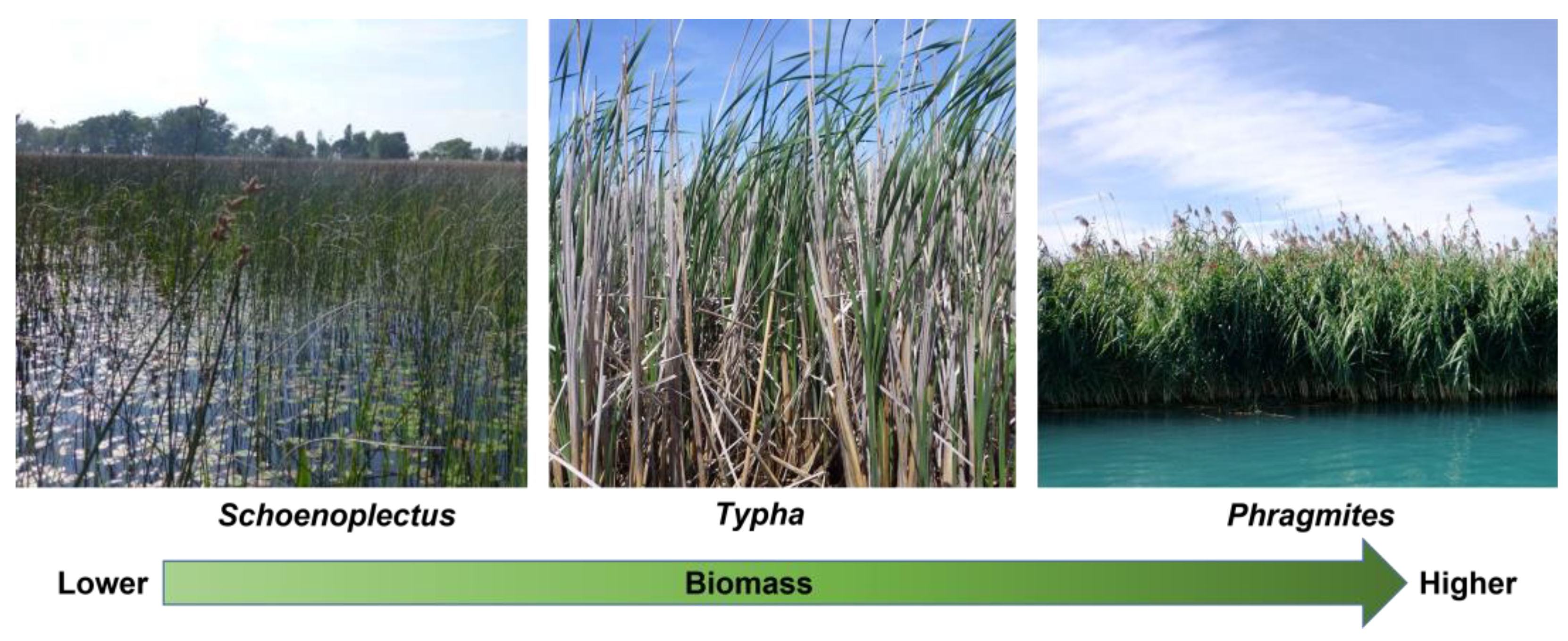
Typha is described as a stout stemmed emergent wetland species, often growing in dense clumps. It has broad linear leaf blades and a distinguishable brown cylindrical flowering spike. Phragmites is a perennial grass, with a stiff thin central stem and many wide leaves forming along the length of the central stem. The plumy inflorescence at the top of the stems often has a purplish hue. Schoenoplectus is a sedge known as bulrush with a thin (~1–2 cm diameter) cylindrical mainstem 1–3 m tall typically growing in deeper water than Phragmites and Typha, up to 1.5 m [10]. But plants as tall as 4.2 m have been found in even deeper water [11]. The only leaves are small and near the base of the plant. The inflorescence forms in a terminal panicle at the end of the stem but appears to come from the side of the stem. Schoenoplectus, Phragmites and Typha are all clonal through rhizomatous root systems and often form monocultures. There is a general trend of increasing density, height and biomass of these species (Figure 3).
The two study locations are heavily diked for wetland management and in July 2021, much of the Lake Erie wetlands inside the dikes were under a drawdown of water, leaving many with atypical low or no standing water. The St. Clair Delta had typical water level conditions for the wetland complexes.
Figure 3.
Field photos of the three dominant monoculture emergent wetland types found in the lower Great Lakes, with increasing biomass from left (often sparse Schoenoplectus or bulrush) to common cattail (Typha spp.) to the invasive, often tall dense Phragmites australis.
Figure 3.
Field photos of the three dominant monoculture emergent wetland types found in the lower Great Lakes, with increasing biomass from left (often sparse Schoenoplectus or bulrush) to common cattail (Typha spp.) to the invasive, often tall dense Phragmites australis.
2.2. Field Data Collection Methods
Field data were collected in support of the ASAR mission from a variety of field locations coincident to the overpasses in the St. Clair River Delta and wetlands of western Lake Erie. Field data on extent of inundation, water levels, height, density and biomass of different wetland vegetation types, canopy closure, and other wetland characteristics were sampled to assist us in interpreting the signatures of L-, S- and C-band radar data to address our research questions.
Field locations in the St. Clair River Delta and Western Lake Erie were visited the week of 14 July of 2021. Using 2019 base maps produced from 3 dates of Radarsat-2 PolSAR data and 3 dates of WorldView-2 imagery [12,13], we randomly selected field locations across the study area within 1 km from access points via a road or water body (via boats). Each site was minimally 20 m x 20 m in size of fairly homogeneous ecosystem type to be commensurate with the resolution of the SAR systems and accounting for speckle reduction. At each site general ecotype was recorded (shrub, emergent, open water, upland, floating aquatic), percent cover of vegetation, open water, exposed soil, dominant and sub-dominant species present. For the monoculture sites of Phragmites, Schoenoplectus and Typha, we sub-sampled three 30 cm x 30 cm subplots that were randomly selected for measuring the number of stems by species separated by live and dead condition. Of these stems, 3 representative live individuals were measured for stem height, basal diameter, diameter at water level, and diameter at 1 m height above water along with water depth with a date/time and GPS stamp. Notes on whether vegetation was tilted from wind or fallen/knocked down were made as well as insect damage, herbicide, or cut vegetation. As part of the protocol, GPS tagged photos were taken at each site center, in four cardinal directions, nadir and straight up. Vegetation biomass data were acquired at 27 sites in the St. Clair River Delta and 15 sites in the wetlands of western Lake Erie. Additional data were collected in wetlands without the presence of the three types of interest (Figure 1).
For biomass estimation, unpublished allometric equations were used from University of Michigan’s database for Schoenoplectus and Typha. For Phragmites, no equations existed so we harvested Phragmites stems from 2 locations (20 stems) and developed a new biomass equation based on height of vegetation.
Phragmites biomass, where x is height in m:
Schoenoplectus biomass, where x is height in cm:
Typha biomass, where x is volume in cm3:
2.3. Remote Sensing Data Processing
ASAR data collected on 14 July 2021 over the Great Lakes study areas were distributed as Level 1 Single Look Complex (SLC) data and Level 2 Geocoded Amplitude Images. We downloaded Version 1.3B Level 1 and Level 2 data from NASA’s JPL website (https://uavsar.jpl.nasa.gov/cgi-bin/asar-data.pl). Level 2 data were calibrated to Sigma Nought () intensity using the following calibration algorithm:
where DN represents pixel values in the provided GeoTIFFs, ip is local incidence angle (provided as an ancillary dataset), N is the noise bias for each polarization, and KdB is the calibration constant. Noise bias and calibration constants were provided in associated metadata. Although the product was geocoded, there were some geolocation errors so additional manual georeferencing was applied by visually interpreting tie points between the SAR data and high resolution optical airphotos. For this process, we utilized USDA NAIP images collected in 2020 and 2021.
For polarimetric data analysis, we extracted SLC data from the provided HDF5 files and used PolSARpro software (v. 6.0) to apply a Refined Lee Polarimetric Filter with a 7 × 7 pixel window size to both L- and S-band data. Three polarimetric decompositions were applied to the quad polarized data. First was the van Zyl et al. [14] NNED decomposition similar to the Freeman and Durden [15] decomposition but with correction for non-negative eigen vectors in the algorithm, producing double, volume and single bounce scattering. Second was the Cloude and Pottier [16] decomposition that produces Entropy, Anisotropy and Alpha Angle parameters. Lastly, was a decomposition specifically designed for vegetation mapping, the Neumann et al. [17] decomposition which produces three polarimetric parameters: Delta, Tau, and Delta Phase. Georeferencing information extracted from the HDF5 files was used to geocode the polarimetric results. Like the Level 2 products, manual georeferencing was required to ensure geolocational accuracy of the output data.
For C-band Radarsat-2 (R-2) FQ10W data over Lake St. Clair and FQ62 over western Lake Erie were acquired on 26 July 2021, under a USFWS cooperative agreement. SLC data were provided for the quad-pol imagery and similar processing was performed as the L- and S-band, however, for R-2 data both PCI and PolSARpro were used, applying radiometric terrain correction in PCI. In this case post-processing geolocation with tie points was not necessary.
2.4. Ecotype Mapping
Polarimetric decomposition components for S- and L-band were used as inputs in a Random Forests [18] classifier which has proven effective with L-band [19]. Training and validation data for the model were derived from a combination of field data and interpretation of USDA NAIP aerial imagery. 80% of training polygons were randomly selected for training and the remaining 20% were reserved as an independent validation dataset. The model was run in a Python 3.0 environment using the Sci-kit Learn package. The model was initiated with default parameters except for the number of trees, which was set to 500.
2.5. Assessment of Scattering Models
To assess the accuracy of established scattering models we generated additional polygons representing 10 m x 10 m areas of Typha and Phragmites across a range of incidence angles from the Lake St. Clair dataset. We then extracted local mean local incidence angle and the mean of each scattering type from the van Zyl NNED decomposition products to compare expected vs. observed scattering behavior.
We created co-pol phase difference histograms of the three dominant wetland monocultures, using 2019 multi-date Radarsat-2 and Worldview basemaps [12,13] to determine extent of each across the St. Clair River Delta ASAR images. These were produced similarly to Atwood et al. 2020 and Ahern et al. 2022 and allow us to assess the dominant scattering type occurring via the expected co-pol phase difference (CPD). Surface scatter ideally has an expected CPD of 0°, double bounce scattering has expected CPD of 180°, while volume scatter has an expected uniform distribution from CPD -180° to 180°.
2.6. Assessment of Vegetation Structure Limitations
To assess vegetation structure and biomass limitations on our ability to monitor inundation we applied a thresholding method to distinguish flooded vegetation from open water and non-inundated areas [12]. The method involves using cross-polarized backscatter to separate open water from land via thresholding, and then using the cross-polarized ratio (HH/VH or VV/VH) to distinguish flooded vegetation from non-flooded vegetation. In this case we incorporated both VV/VH and HH/HV to quantify flooded vegetation extent. We also assessed the relationship between total live and dead biomass and backscatter from the different frequencies and polarizations to determine which had strong relationships to biomass and whether developing biomass retrieval algorithms for wetlands in the Great Lakes was feasible.
3. Results
3.1. Field Data
For assessment of how well the three SAR frequencies are able to detect inundation and limitations due to biomass and density, 46 field sites were sampled. A total of 31 sites were visited in the St. Clair delta ASAR footprint and 15 sites in the Western Lake Erie footprint (Table 1) including 9 Schoenoplectus dominated sites, 16 Phragmites dominated sites and 22 Typha dominated sites. Mean height of vegetation ranged from 1.36 to 2.89 m, live biomass ranged from 16.2 to 7336.5 g/m2, and dead standing biomass from 0.0 to 9755.4 g/m2 (Table 1).
3.2. Ecotype Mapping: Can L-Band and S-Band polSAR Data be Used to Map Wetland Ecotypes with High Accuracy?
Using the backscatter and decomposition components in the random forests classifier, individual S-band maps had lower accuracy than the L-band maps, but a combination of the two frequencies produced the greatest accuracy (Table 2 and Table 3). The L- and S-band classification for the St. Clair Delta resulted in 92% overall accuracy, with very high accuracies for the invasive monocultures and all wetland types (>79% user’s and >73% producer’s accuracy) except wet meadow which was sometimes confused with agriculture (84% user’s and 46% producer’s accuracy, Table 2). The L- and S-band classification for the Western Lake Erie study area had lower overall accuracy, 76%, with comparable user’s accuracies (>85% for invasive monocultures) but significantly lower producer’s accuracies (38–82%, Table 3) than for St. Clair. In comparison to the previous base maps produced with multi-date polarimetric Radarsat-2 and Worldview (R-2/WV) circa 2019, the L- and S-band single date map of St. Clair is comparable in overall UA and PA accuracies, with improved accuracies for the 3 monoculture species, except PA for Schoenoplectus (Table 2). For Western Lake Erie, the L- and S-band maps are of lower accuracy than the R-2/WV 2019 maps (Table 3). Figure 4 shows the six maps generated from the S-, L-, and combined S- and L-data for each study area. S-band is overestimating the forest and shrub and urban classes in both study areas, where there is significant confusion with the agriculture/grass class. The agriculture/grass class is also often confused with the wetland classes. This is especially prevalent at L- and combined L- and S-band maps for the W. Lake Erie study area, where agriculture is much more common land use, and many crop fields are misclassified as wet meadow. Phragmites and Typha were also occasionally incorrectly identified in crop fields in both areas, especially at S-band. Notably, there was little confusion between Phragmites, Typha, and Schoenoplectus. Phragmites and Typha were confused with each other most often in S-band classifications, but confusion was minimal in the L-band and combined S- and L-band maps. In both areas the most common class confused with Schoenoplectus was open water. The S- and L-band combination performed best at identifying Schoenoplectus in the St. Clair Delta, but was outperformed by L-band alone in W. Lake Erie.
3.3. Assessment of Scattering Models: Do Established Scattering Models Explain Polarimetric L- and S- Band SAR Interactions with Wetlands?
Assessing three-component decompositions [14,15,20] at C-band, we found previously that double bounce scattering was misattributed as single bounce due to the static threshold of co-polarized phase difference in the algorithms [4,5]. The S- and L- band ASAR data has a wide range of incidence angles transitioning from 26° to 53° over a swath width of approximately 10 km. We found incorrect classification of double-bounce scattering was evident especially at shallow (large) incidence angles at L-band, with attribution as single bounce scattering becoming noticeable at approximately 35° and becoming completely misattributed at approximately 40°. At S-band, the misattribution was less pronounced across incidence angles but exhibited similar trends as the L-band data (Figure 5). In some cases, flooded Phragmites stands exhibited dominant volume scattering at C- and S-band. At L-band, double-bounce scattering is dominant at steep (small) incidence angles, while volume scattering again dominates shallow angles.
A comparison of the Van Zyl NNED 3 component decomposition to CPD for a region of the St. Clair Delta demonstrates the variability in double bounce across the scene from near to far range (Figure 6).
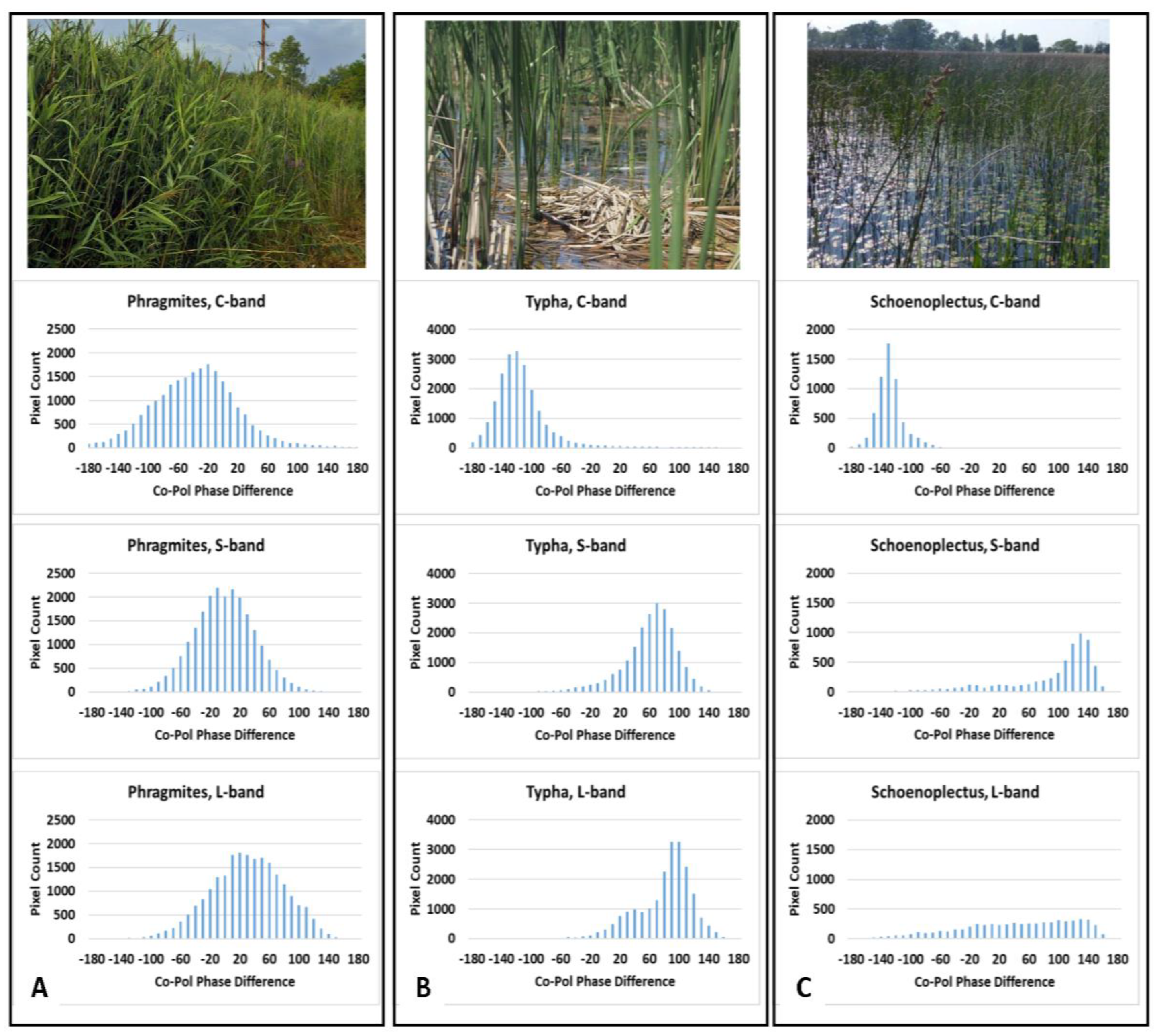
Co-Pol Phase Difference (CPD) histograms (Figure 7) aid in determining dominant scattering mechanisms across the dominant wetland types. We found that for the simpler structured cylindrical stems without leaves along the main stems, double bounce phase difference appeared to dominate for both Typha and Schoenoplectus for C- and S-band, but for L-band the stems of Schoenoplectus are likely too thin and sparse, thus the expected CPD of +/-180° indicative of double bounce scattering is not exhibited. However, there is a characteristic ~180° shift for Typha at L-band. For all 3 frequencies, surface (single bounce) scattering is dominant for Phragmites.
Figure 6.
NNED 3 component (double bounce, volume scatter, surface bounce) decomposition compared to the CPD at (a) C-band, (b) S-band and (c) L-band for a subsetted area of St. Clair Delta. Incidence angle ranges from 26° to 48°. (d) For reference the 2019 multi-sensor (Radarsat-2 C-band and Worldview) map showing the dominant cover classes is shown with a legend below it.
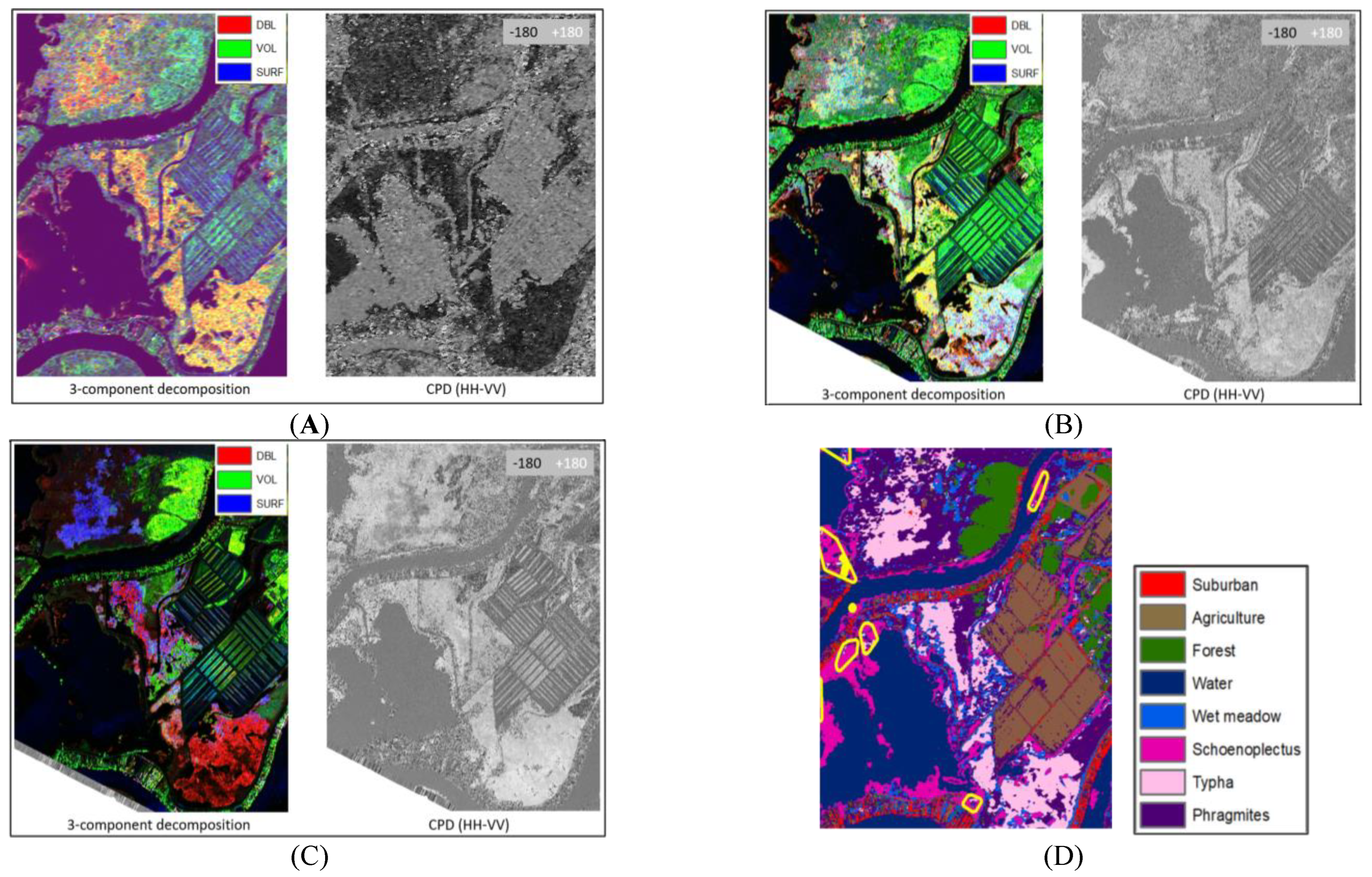
Figure 7.
Co-pol phase difference (CPD) histograms for each of the three dominant monoculture species by frequency. (a) A characteristic photo of Phragmites and the histograms for C-band (top), S-band (middle) and L-band (bottom); (b) A characteristic photo of Schoenoplectus with histograms for C-, S-, and L-band; (c) A photo of Typha followed by the histograms for C-, S- and L-bands.
3.4. Assessment of Vegetation Structure Limitations: What are the Vegetation Structure Limitations of Different Radar Wavelengths for Wetland Inundation?
Scattering interactions with three most common wetland genera in the lower Great Lakes, Typha, Phragmites and Schoenoplectus, varied with frequency. For Schoenoplectus, characterized by sparse, thin cylindrical spikelike stems which emerge from the water, we found that even in dense stands, which are indicative of shallower water, L-band exhibits low backscatter at all polarizations (Figure 8), that is not much different from the open water response. However, for the shorter wavelengths of S- and C- band stronger responses are exhibited, particularly for the like-polarizations. Typha has a thick central stem with basal leaves spiraling upwards. Each of the three frequencies exhibits a strong, but unique response from Typha, with a greater VV backscatter response at L-band over HH, and the opposite for S- and C-band. Phragmites, which has a thin central stem with alternating leaves the full length of the stem, forms extremely dense monotypic stands in these southern Great Lakes sites. It has lower backscatter returns for all 3 frequencies than Typha, likely due to the high biomass which can be less penetrable for some SAR frequencies.
Inundation algorithms were applied to each frequency and showed some differences between frequencies. The L-band inundation classification produced the largest estimate of inundated area in the St. Clair Delta, followed by C-band, then S-band (Table 4). This estimate is slightly misleading, as the backscatter in S- and L-band is significantly impacted by incidence angle effects. Far range incidence angles over 50 degrees showed poor results, especially at L-band due to misattribution of double bounce scatter. S-band was less impacted by shallow incidence angles, as evidenced by the extensive classification of inundated area in St. John’s Marsh, in the northern portion of the St. Clair Delta study area (yellow of Figure 9).
C-band performed best at detecting flooded Schoenoplectus. S-band and L-band were able to detect some dense stands of Schoenoplectus but often the sparse stands were classified as open water.
C-band was not able to detect flooding beneath mature Phragmites stands in many cases. S- and L-band had better success at detecting flooded Phragmites but were still limited in some cases, especially when mats of dead vegetation were present above the water, or where wind had blown the stalks over so the vertical structure was not as prominent. All frequencies were generally capable of detecting flooding beneath immature Phragmites, as well as monotypic stands of Typha.
When we compared inundation extent maps with field data, S-band was slightly more accurate than C- or L-band, correctly assessing inundation status at 35 of 42 sites (83.3%). C-band was able to accurately detect inundation at 34 of 42 sites (80.9%), while L-band was correct 33 out of 42 times (78.5%).
Plots of stand biomass vs. HH backscatter by frequency (Figure 10) showed the strongest relationship for L-band (R2 0.71). When the non-flooded sites were added to the plots, relationships became weaker, with more outliers (not shown). For the cross polarization, C-band had the strongest R2, S-band was also high but had one site with backscatter below the noise floor. These plots show that biomass is influencing the backscatter, with a general trend of increasing backscatter with increasing biomass. As biomass and water level vary, the dominant scattering mechanisms are likely changing with different frequencies.
4. Discussion
One of the most accurate methods to produce wetland ecotype maps is using a combination of radar and optical multi-season data [21,22]. This allows for the capture of phenological differences in the ecotypes from spring, summer and fall and also differences in structure and inundation condition from radar. We found that fully polarimetric S- and L- band SAR data from a single date can be used to effectively identify the extent of various wetland plant genera and ecotypes common in the Great Lakes without the use of other data sources, such as optical or thermal imagery. This has a great advantage for timely mapping in locations like the Great Lakes that are often cloud covered. Other researchers have had success in mapping wetland marsh with single date C-band [23] and L- and C-band [24] polSAR decompositions using machine learning and deep learning classifiers. Fu et al. 2023 found L-band to outperform C-band and decompositions to outperform backscatter coefficients in their deep learning algorithms with best overall accuracies of 86-88%. C-band polSAR decompositions were found suitable for mapping a wetland area in China where there were only 2 wetland ecotypes, and both had very low stature biomass herbaceous vegetation (Suaeda salsa and Spartina alterniflora) [23]. They found the C-band decompositions to allow classifications with overall accuracies of 78 to 93 percent and wetland class accuracies between 63 and 94 percent, depending on the model.
Our results show concurrent multi-frequency SAR collections can perform as well as multi-season approaches, which reduces latency time for wetland mapping significantly. In regions with high cloud cover, multi-source wetland type identification could require imagery from multiple years if seasonal cloud-free imagery is unavailable. Thus, the timely nature of cloud-penetrating SAR data being collected routinely will allow for mapping wetland types and monitoring wetland condition during key periods of importance, e.g., during important breeding or nesting habitat seasons which can be of very short duration. Overall accuracy of wetland type maps created with combined L- and S- band data and machine learning classifiers was approximately 92% for the St. Clair Delta. This is comparable to accuracy estimates achieved with combinations of three season optical and C-band SAR imagery [12]. Lower accuracies were achieved in the Western Lake Erie study area which is likely due to non-flooded condition of wetlands. Many of the major wetland complexes in the region are diked with artificially manipulated water levels. During the time frame of the ASAR data collection, many of these Lake Erie areas had been drawn down to very low or zero water levels. This observation indicates that inundation status is a key factor in the ability to accurately identify wetland monocultures in the Great Lakes from a single date of polSAR imagery. Scattering signatures are more differentiable under flooded conditions due to double bounce scattering from the water and vegetation. In non-flooded conditions, double bounce scattering is greatly reduced and surface or volume scatter prevails. This results in confusion to upland classes of similar vegetation structure. This is highlighted by the relatively low accuracies of non-flooded cover types in both study areas, namely the agriculture/grass class, which was often confused with the wet meadow class. Wet meadows tend to have wet or saturated soils but water tables mid-summer are typically below the surface. Since agricultural areas are often irrigated in the Great Lakes and are also monocultures, the confusion with wet meadow is unsurprising. Similarly, the developed class had low accuracies. In the St. Clair Delta, there was often confusion between the developed class with wetland classes, particularly Phragmites. In W. Lake Erie, the developed class was confused with several classes. This result is likely due to the large in-class variability of the area, with heavy industrial activity and urban environments in and near Toledo, and extensive low-density residential areas throughout the region that causes double bounce from the human built structures. The high accuracies achieved for Schoenoplectus with L-band data were somewhat surprising considering the often sparse distribution of Schoenoplectus stems. It is important to note that only two sites with Schoenoplectus were visited in the W. Lake Erie study area, so additional patches were identified with interpretation of high-resolution aerial imagery. Although the aerial imagery was collected during the same summer as the ASAR overpasses, they were not coincident, so there is likelihood some Schoenoplectus training samples were not representative of the class, and instead were more representative of open water, which would explain the confusion in the classified maps. However, double bounce from wind-drawn capillary waves could also be a cause of confusion.
Common decomposition methods are prone to misattribution of dominant double bounce scattering type to surface scatter under certain vegetation moisture and SAR geometry conditions. Our analysis shows that this misattribution occurs at S- and L-band, similar to previous research at C-band [4,5]. Observed scattering behavior related to incidence angle (Figure 5 and Figure 6) and vegetation structure (Figure 7) was generally consistent with published models of microwave scattering from dielectric cylinders [4,5]. When the anomaly will occur is a function of the radius of the vegetation stems (i.e., cylinders) relative to the wavelength [5] and the moisture in the plants. Low moisture in the vegetation results in larger anomalies [5]. Using a time-series of NISAR data may allow for monitoring wetland plants for moisture status by using the appearance of these anomalies, such as during the onset of senescence in the fall season, or when the vegetation becomes stressed during drought or other circumstances which cause water level changes.
Our results showed, that detection of flooding beneath the 3 dominant species that often form monocultures (Phragmites australis, Schoenoplectus acutus, and Typha spp.) was dependent on frequency in relation to the biomass and structure of the vegetation (Figure 9, Table 4). C-band, the shortest wavelength studied, performed best for detecting flooded Schoenoplectus which has the sparsest and simplest structure. L- and S-band were able to detect flooding beneath the high biomass, dense Phragmites canopies, where C-band was limited similar to previous findings with C- and L-band [25]. Lamb et al. 2025 found L-band backscatter thresholding to work well in mapping inundation in coastal salt marshes with varying marsh vegetation including Phragmites australis, Typha spp., Spartina and Schoenoplectus with accuracies around 90% or better for L-HH or L-VV. They found limitations in C-VV backscatter thresholding from Sentinel-1 and suggest for C-VV data that it is best to use change detection classification from different tidal stages which produced higher accuracy (76%) maps. Radiometric modeling conducted by those authors (Lamb et al. 2025) demonstrated that C-HH (as available from Radarsat-2) is more sensitive to inundation and surface changes than VV polarization (i.e., Sentinel-1). We found all three frequencies studied (L, S, and C) were able to detect flooding beneath Typha canopies and immature Phragmites stands. Thus, a single frequency system is going to have errors due to mismatch of wavelength to vegetation stem size, density, height and biomass. Thus, a combination of frequencies would be optimal for monitoring inundation extent to capture flooding beneath a range of canopy types and vegetation structure.
Lastly, we found for the flooded marsh wetlands, that we could produce a biomass retrieval algorithm from the SAR polarized data, with the strongest relationship for L-HH (R2 = 0.71), followed by C-HV (R = 0.66) and S-HH (R2 = 0.63). This is important for monitoring changes in plant biomass over a growing season and in combination with wetland type maps would allow for assessing wildlife habitat and nesting grounds. Further, it is important for estimating C-storage in wetland vegetation and for National Greenhouse Gas Inventories [26].
Limitations
The polarimetric signature analysis of ASAR co-pol and cross-pol channels for both L- and S-band shows that perfect behavior is shown by the co-pol signature but distortions were easily identified in the cross-pol signatures [27]. These distortions may impact polSAR decompositions, with either under or over-estimation of scattering elements. Since these over or underestimations of scattering elements may be wetland cover type dependent, it did not seem to adversely affect our ability to map wetland classes. Further, the CPD analysis did not include the cross polarized data, but allowed us to assess dominant scattering mechanisms and relate that to the three component modeled decompositions.
There were limitations in our field data set that should be expanded for further analyses. Observations of wetland sites with non-inundated wet soil condition was limited and should be explored further. We found that the SAR biomass retrieval algorithms had higher accuracies when the non-inundated wetlands were withheld, however the number of non-inundated wetlands sampled was low, preventing a similar analysis for non-inundated wetland biomass retrievals. In addition, we had limited shrub wetlands that were sampled in the field and a lack of samples for forested wetlands. SAR monitoring limitations in woody wetlands need to be further explored and the threshold classification technique for marsh vegetation is likely not suitable for forested wetlands, and instead a change detection approach may be necessary [25].
5. Conclusions
High temporal resolution multi-frequency (e.g., L-, S- and C-band) SAR dual polarization and quad polarization data will greatly improve capabilities of mapping wetland ecotypes and monitoring hydrological condition. Cloud cover is often a limiting factor in obtaining timely data for monitoring. SAR provides the ideal tool for monitoring in a routine and timely fashion for such an environment. The additional knowledge gained from routine 6-12 day repeat NISAR collections will improve coastal wetland monitoring capability which is of key importance as water level fluctuations and invasive species encroachment continue to alter the land-water interface. Monitoring information will be important for management decisions in areas with significant human populations, areas vital for wildlife habitat conservation or restoration and for planning for coastal resiliency. In addition, routine monitoring of wetland extent changes through time will allow for detection of wetlands connected to the Great Lakes via surface and ground water. This is important because connectivity to the Great Lakes defines coastal wetlands, which are affected by large lake processes and regulated differently than non-coastal wetlands.
While, C-band data have been routinely available from Sentinel-1 since 2015, it is limited to dual polarization (VV/VH) with penetration limitations in higher biomass wetlands. NISAR is planned to be quadrature polarization over the Great Lakes, allowing for continuation of many of the methods developed in this research to be used for monitoring. S-band data will not be available over this region, but combining Sentinel-1 and or quad polarization RCM or Radarsat-2 with NISAR L-band, will provide powerful tools for monitoring wetland health of the Great Lakes.
In this study we confirmed anomalous behavior of decompositions at L-, S- and C-band which allow for understanding uncertainties and limitations of inundation maps and classification maps. It also has implications for repeat pass InSAR applications for water level changes which requires high coherence between successive image dates. Ahern et al. [5] recommend choosing radar wavelengths that are considerably shorter, or longer, than the diameters of the wetland plant stems of interest to avoid resonance effects in double-bounce backscatter. The anomaly can appear as “holes” in the imagery due to large drops in backscatter, or changes in the dominant scattering mechanism.
This study provides an advancement in understanding of polarimetric SAR for studying wetlands, which has applications for improved estimates of wetland extent, wetland type, water level changes, wetland biomass and wetland contributions to Carbon cycling.
Funding
This work was supported by NASA ISRO-ASAR Grant # 80NSSC20K0679 and USFWS Cooperative Agreement # F18AC0039 (Great Lakes Restoration Initiative (GLRI) -funded).
Data Availability Statement
Field data and map products will be made available upon request. ASAR data are available from NASA JPL https://uavsar.jpl.nasa.gov/cgi-bin/asar-data.pl. Radarsat-2 data are unable to be shared publicly by the authors given restrictions in the data access agreement.
Acknowledgments
We acknowledge the field teams who assisted in collecting all of the data for this analysis including Dorthea Vander Bilt, Karl Bosse, Charlotte Weinstein, Andrew Poley, Mary Ellen Miller, and Vanessa Barber. We thank Don Atwood for his review of the manuscript and suggested edits and Nicole Kozel for assistance in formatting and editing text and figures.
Conflicts of Interest
The authors declare no conflicts of interest. The NASA funding agency encouraged publication of the study results but they had no role in the design of the study; in the collection, analyses, or interpretation of data; in the writing of the manuscript; or in the final decision to publish the results.
Abbreviations
The following abbreviations are used in this manuscript:
| SAR | Synthetic Aperture Radar |
| NISAR | NASA-ISRO Synthetic Aperture Radar |
| PolSAR | Polarimetric SAR |
| CPD | Co-polarized phase difference |
| ASAR | Airborne Synthetic Aperture Radar |
| NASA | National Aeronautics and Space Administration |
| ISRO | Indian Space Research Organization |
| USFWS | United States Fish and Wildlife Service |
References
- Environment Canada Where land meets water: understanding wetlands of the Great Lakes; Environment Canada, 2002.
- Gronewold, A. D.; Rood, R. B. Recent Water Level Changes across Earth’s Largest Lake System and Implications for Future Variability. Journal of Great Lakes Research 2019, 45(1), 1–3. [Google Scholar] [CrossRef]
- Atwood, D.; Battaglia, M.; Bourgeau-Chavez, L.; Ahern, F.; Murnaghan, K.; Brisco, B. Exploring Polarimetric Phase of Microwave Backscatter from Typha Wetlands. Canadian Journal of Remote Sensing 2020, 46(1), 49–66. [Google Scholar] [CrossRef]
- Ahern, F. J.; Brisco, B.; Battaglia, M. J.; L. Bourgeau-Chavez; Atwood, D.; K. Murnaghan. SAR Polarimetric Phase Differences in Wetlands: Information and Mis-Information. Canadian Journal of Remote Sensing 2022, 48 (6), 703–721. [CrossRef]
- Ahern, F.; Brisco, B.; Murnaghan, K.; Lancaster, P.; Atwood, D. K. Insights into Polarimetric Processing for Wetlands from Backscatter Modeling and Multi-Incidence Radarsat-2 Data. IEEE Journal of Selected Topics in Applied Earth Observations and Remote Sensing 2018, 11(9), 3040–3050. [Google Scholar] [CrossRef]
- Hong, S.-H.; Shimon Wdowinski. Double-Bounce Component in Cross-Polarimetric SAR from a New Scattering Target Decomposition. IEEE Transactions on Geoscience and Remote Sensing 2013, 52 (6), 3039–3051. [CrossRef]
- Siqueira, P. L- and S-Band Polarimetric Data Collections by ISRO’s ASAR Instrument in Support of NISAR Ecosystems Algorithm Development. IGARSS 2022–2022 IEEE International Geoscience and Remote Sensing Symposium 2022, 7468–7470. [CrossRef]
- Albert, D. A. Between Land and Lake: Michigan’s Great Lakes Coastal Wetlands; Michigan Natural Features Inventory, 2003.
- Wilcox, D.A, Thompson, T.A., Booth, R.K., and Nicholas, J.R.; Lake-level variability and water availability in the Great Lakes; Circular 1311; U.S. Geological Survey 2007 https://pubs.usgs.gov/circ/2007/1311/pdf/circ1311_web.pdf.
- Tilley, D. Plant guide for hardstem bulrush (Schoenoplectus acutus), 2012.
- Reznicek, A. A.; Voss, E. G.; Walters, B. S. University of Michigan. https://michiganflora.net/genus/schoenoplectus (accessed 2024-01-26).
- Battaglia, M. J.; Banks, S.; Amir Behnamian; Bourgeau-Chavez, L.; Brisco, B.; Corcoran, J.; Chen, Z.; Huberty, B.; Klassen, J.; Knight, J.; Morin, P.; Murnaghan, K.; Pelletier, K.; White, L. Multi-Source EO for Dynamic Wetland Mapping and Monitoring in the Great Lakes Basin. Remote Sensing 2021, 13 (4), 599–599. [CrossRef]
- Bourgeau-Chavez, L. L.; Graham, J.; Battaglia, M. J.; White, L.; Klassen, J.; Vander Bilt, D. L.; Poley, A. F.; Pelletier, K.; Brisco, B.; Huberty, B. Great Lakes Remote Sensing ESRI Storymap, High resolution monitoring of coastal Great Lakes wetlands in 4D, 2021. https://mtu.maps.arcgis.com/apps/MapSeries/index.html?appid=2d06583e97844ea892413e2290cbe885.
- Jakob van Zyl; Motofumi Arii; Kim, Y. Model-Based Decomposition of Polarimetric SAR Covariance Matrices Constrained for Nonnegative Eigenvalues. 2011, 49 (9), 3452–3459. [CrossRef]
- Freeman, A.; Durden, S. L. A Three-Component Scattering Model for Polarimetric SAR Data. IEEE Transactions on Geoscience and Remote Sensing 1998, 36(3), 963–973. [Google Scholar] [CrossRef]
- Cloude, S. R.; Pottier, E. An Entropy Based Classification Scheme for Land Applications of Polarimetric SAR. IEEE Transactions on Geoscience and Remote Sensing 1997, 35(1), 68–78. [Google Scholar] [CrossRef]
- Neumann, M.; Laurent Ferro-Famil; Jager, M.; Reigber, A.; Pottier, E. A Polarimetric Vegetation Model to Retrieve Particle and Orientation Distribution Characteristics. HAL (Le Centre pour la Communication Scientifique Directe) 2009. [CrossRef]
- Breiman, L. Random Forests. Machine Learning 2001, 45(1), 5–32. [Google Scholar] [CrossRef]
- Adeli, S.; Salehi, B.; Mahdianpari, M.; Quackenbush, L. J.; Chapman, B. Moving toward L-Band NASA-ISRO SAR Mission (NISAR) Dense Time Series: Multipolarization Object-Based Classification of Wetlands Using Two Machine Learning Algorithms. Earth and Space Science 2021, 8 (11). [CrossRef]
- Yamaguchi, Y.; Moriyama, T.; Ishido, M.; Yamada, H. Four-Component Scattering Model for Polarimetric SAR Image Decomposition. IEEE Transactions on Geoscience and Remote Sensing 2005, 43(8), 1699–1706. [Google Scholar] [CrossRef]
- Mahdianpari, M.; Granger, J. E.; Mohammadimanesh, F.; Salehi, B.; Brisco, B.; Homayouni, S.; Gill, E.; Huberty, B.; Lang, M. Meta-Analysis of Wetland Classification Using Remote Sensing: A Systematic Review of a 40-Year Trend in North America. Remote Sensing 2020, 12(11), 1882. [Google Scholar] [CrossRef]
- Bourgeau-Chavez, L.; Endres, S.; Battaglia, M.; Miller, M.; Banda, E.; Laubach, Z.; Higman, P.; Chow-Fraser, P.; Marcaccio, J. Development of a Bi-National Great Lakes Coastal Wetland and Land Use Map Using Three-Season PALSAR and Landsat Imagery. Remote Sensing 2015, 7(7), 8655–8682. [Google Scholar] [CrossRef]
- Zhang, X.; Xu, J.; Chen, Y.; Xu, K.; Wang, D. Coastal Wetland Classification with GF-3 Polarimetric SAR Imagery by Using Object-Oriented Random Forest Algorithm. Sensors 2021, 21(10), 3395. [Google Scholar] [CrossRef] [PubMed]
- Fu, B.; Li, H.; Liu, M.; Yao, H.; Gao, E.; Sun, W.; Zhang, S.; Fan, D. Performance Evaluation of Backscattering Coefficients and Polarimetric Decomposition Parameters for Marsh Vegetation Mapping Using Multi-Sensor and Multi-Frequency SAR Images. Ecological Indicators 2023, 157, 111246. [Google Scholar] [CrossRef]
- Lamb, B. T.; McDonald, K. C.; Tzortziou, M. A.; Tesser, D. S. Characterizing Tidal Marsh Inundation with Synthetic Aperture Radar, Radiometric Modeling, and in Situ Water Level Observations. Remote Sensing 2025, 17(2), 263–263. [Google Scholar] [CrossRef]
- Byrd, K. B.; Ballanti, L.; Thomas, N.; Nguyen, D.; Holmquist, J. R.; Simard, M.; Windham-Myers, L. A Remote Sensing-Based Model of Tidal Marsh Aboveground Carbon Stocks for the Conterminous United States. ISPRS Journal of Photogrammetry and Remote Sensing 2018, 139, 255–271. [Google Scholar] [CrossRef]
- Kumar, S. Polarimetric Distortion Analysis of L- and S-Band Airborne SAR (LS-ASAR): A Precursor Study of the Spaceborne Dual-Frequency L- and S-Band NASA ISRO Synthetic Aperture Radar (NISAR) Mission. 2022. [CrossRef]
Figure 1.
Study areas within the Great Lakes Basin. Red polygons indicate ASAR swaths and blue dots indicate field locations where data was collected.
Figure 1.
Study areas within the Great Lakes Basin. Red polygons indicate ASAR swaths and blue dots indicate field locations where data was collected.
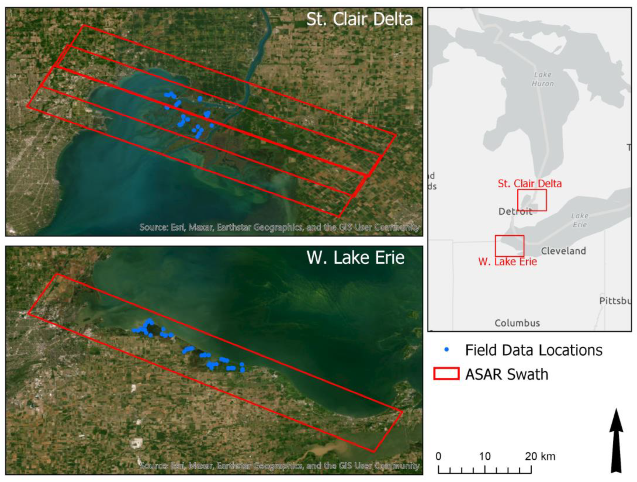
Figure 2.
Generalized zonations of coastal wetlands of the Great Lakes that form due to varying patterns of flooding and wet soils from the dry land to open water from Wilcox et al. [9].
Figure 2.
Generalized zonations of coastal wetlands of the Great Lakes that form due to varying patterns of flooding and wet soils from the dry land to open water from Wilcox et al. [9].
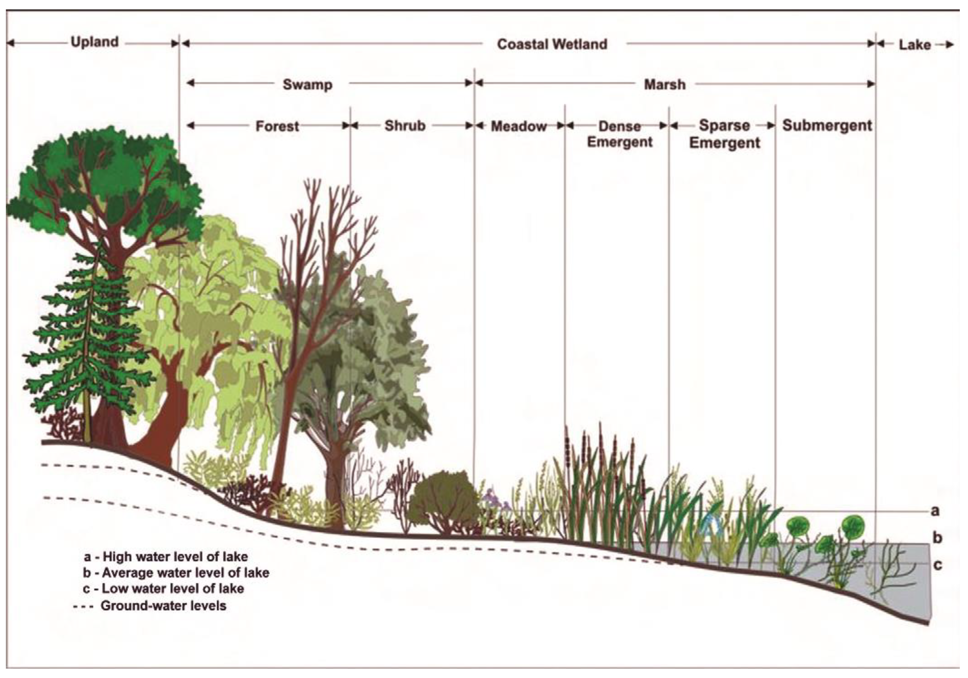
Figure 4.
Classified maps for the St. Clair Delta and W. Lake Erie study areas for S-, L-, and combined S- and L-band data.
Figure 4.
Classified maps for the St. Clair Delta and W. Lake Erie study areas for S-, L-, and combined S- and L-band data.
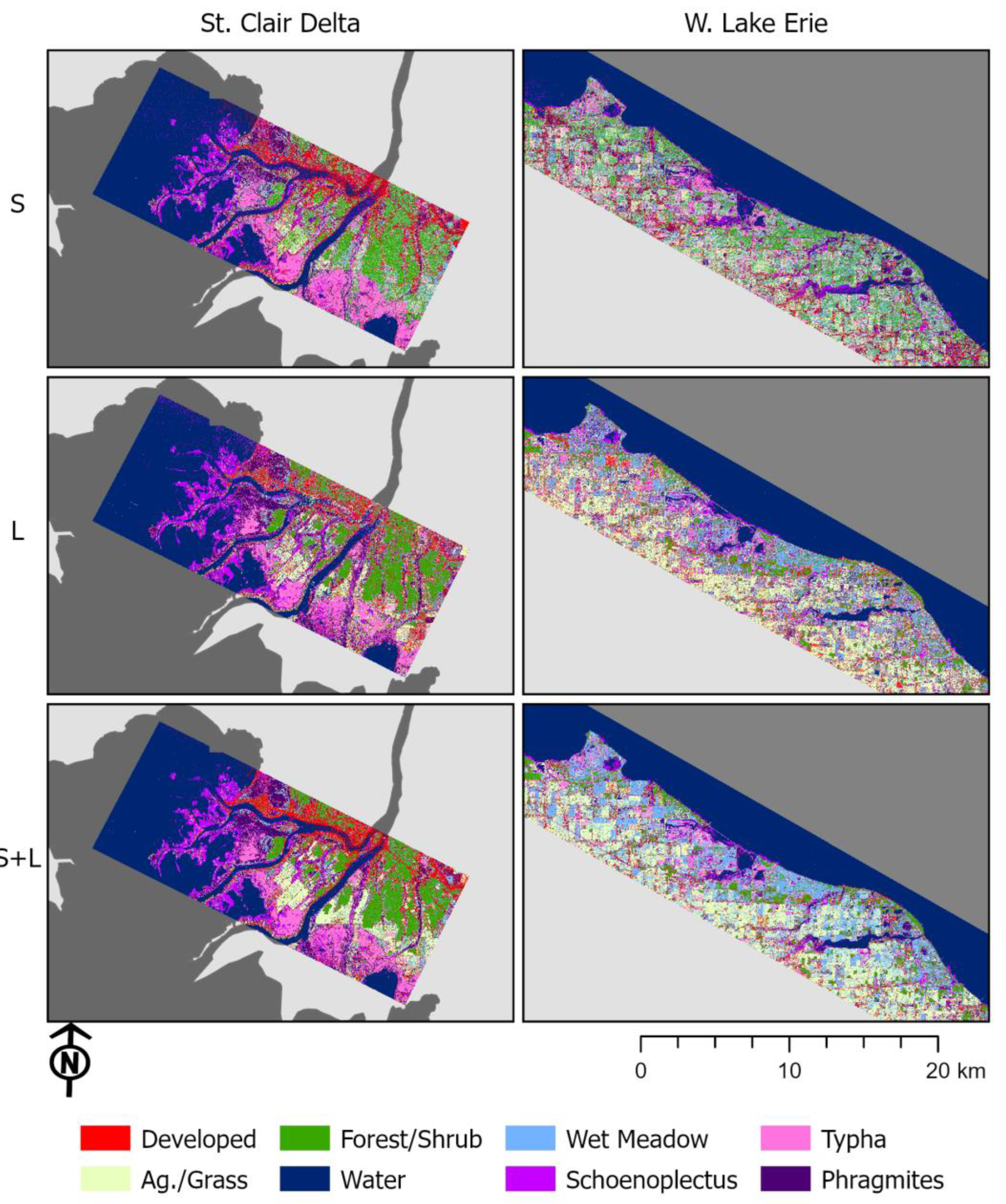
Figure 5.
Co-polarized phase difference vs. Incidence Angle for Phragmites and Typha at L-band. The color scale indicates percentage of double-bounce scattering from the Van Zyl NNED decomposition.
Figure 5.
Co-polarized phase difference vs. Incidence Angle for Phragmites and Typha at L-band. The color scale indicates percentage of double-bounce scattering from the Van Zyl NNED decomposition.
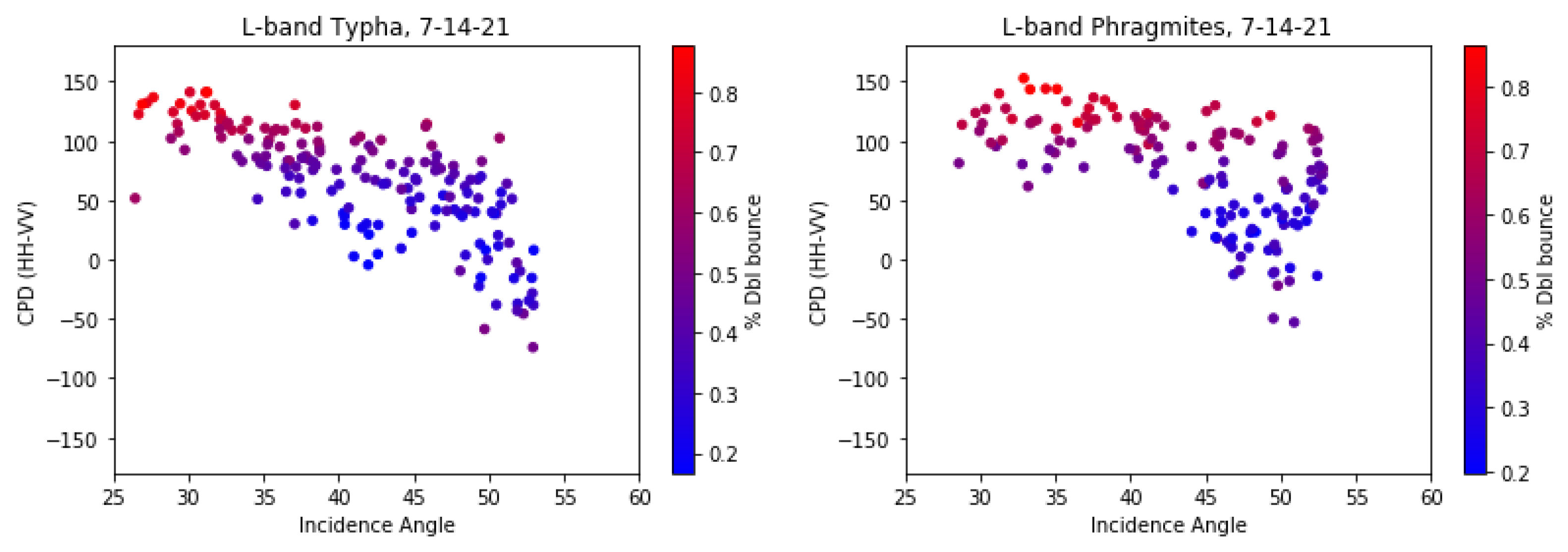
Figure 8.
Boxplots of observed backscatter from three dominant monoculture wetland types and open water for HH, HV, and VV from C-, S-, and L-band.
Figure 8.
Boxplots of observed backscatter from three dominant monoculture wetland types and open water for HH, HV, and VV from C-, S-, and L-band.
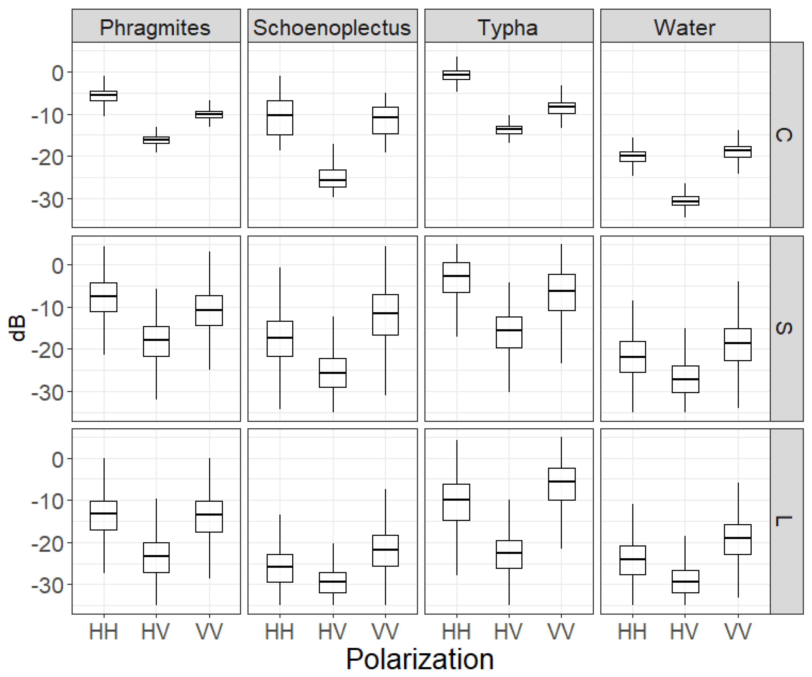
Figure 9.
Flooded vegetation extent in the St. Clair Delta as identified by each frequency. Colors show red areas as only identified by C-band, green as only identified by S-band, blue as only identified by L-band, whereas yellow was identified only by C- and S-bands, purple was identified only by C- and L-bands, cyan areas were only identified by S- and L-bands, and white areas were identified by all 3.
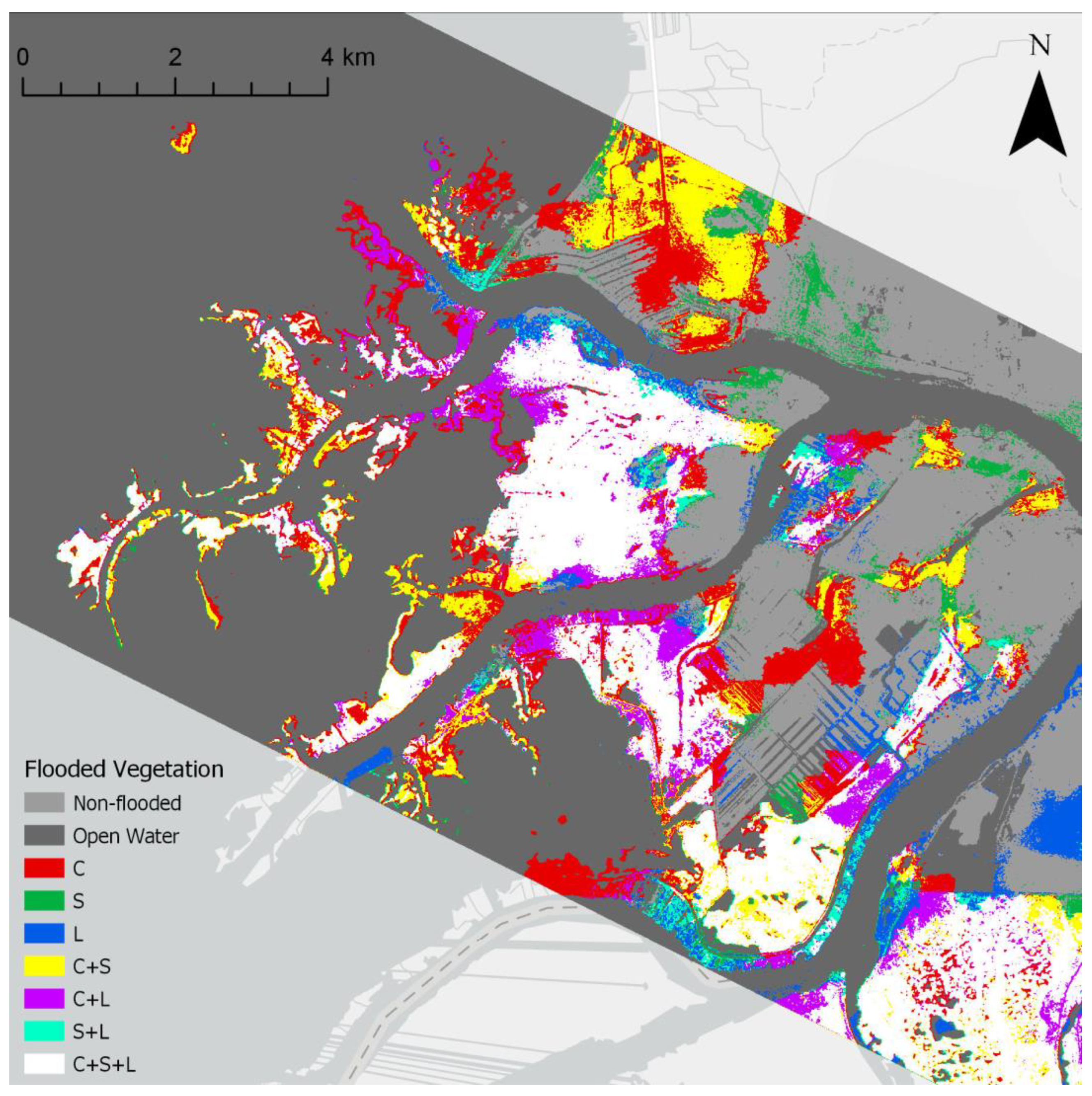
Figure 10.
Plots of (a) HH-backscatter vs. log of biomass for each frequency and (b) HV-backscatter plots for each frequency. Phragmites data are shown in purple, Typha in orange and Schoenoplectus in pink..
Figure 10.
Plots of (a) HH-backscatter vs. log of biomass for each frequency and (b) HV-backscatter plots for each frequency. Phragmites data are shown in purple, Typha in orange and Schoenoplectus in pink..
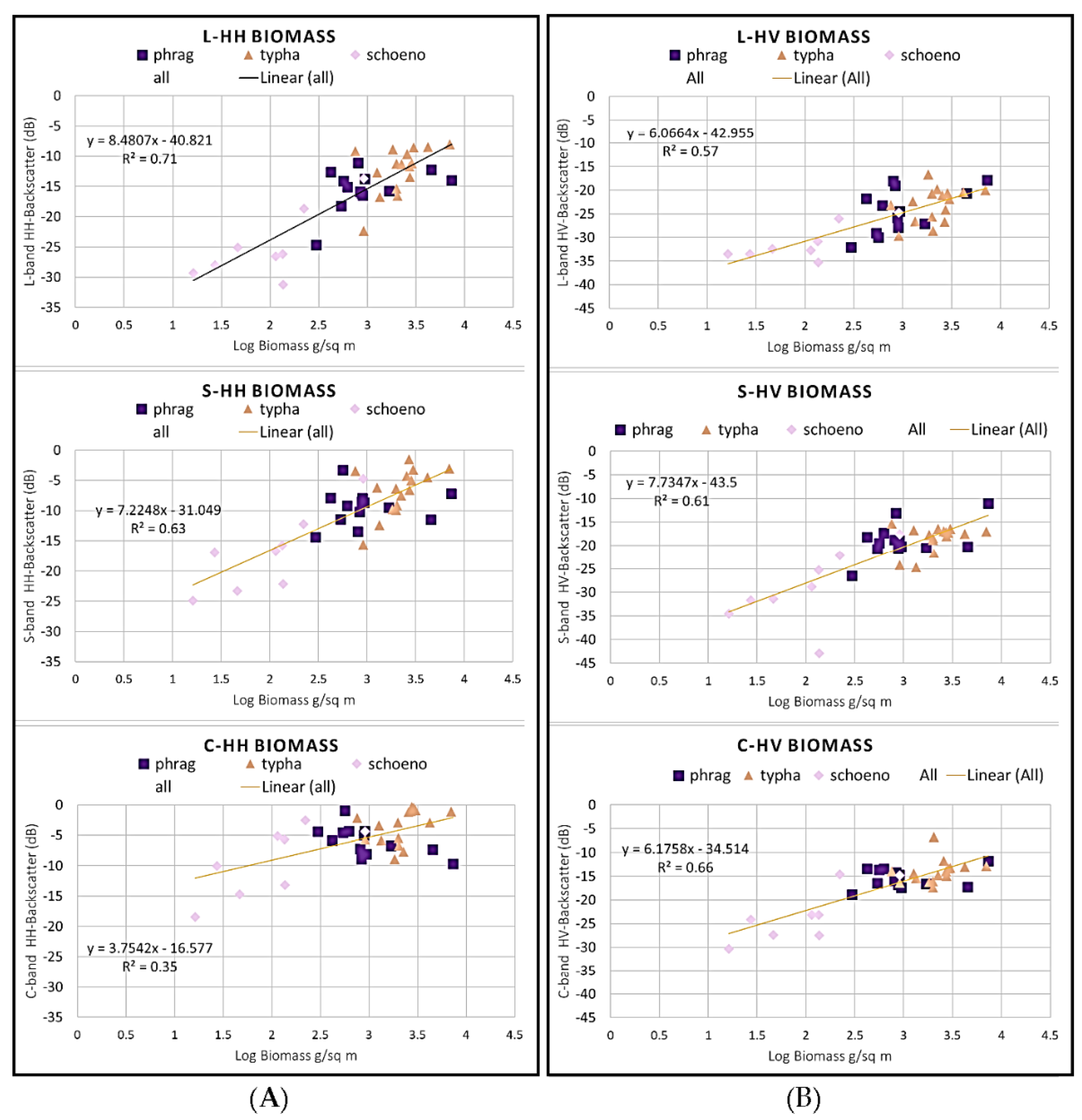

Table 1.
Summary of field collected data on vegetation biomass, heights, diameters, stem densities and water depths at the St. Clair and Erie study areas. Here we show mean values across sites by dominant species (Phragmites, Typha or Schoenoplectus) at each study area.
Table 1.
Summary of field collected data on vegetation biomass, heights, diameters, stem densities and water depths at the St. Clair and Erie study areas. Here we show mean values across sites by dominant species (Phragmites, Typha or Schoenoplectus) at each study area.
| Study Area | Veg Type | n sites | Avg. Height (m) | Avg. Density (stems/m2) | Avg. Stem Diameter (cm2) | Avg. Live Biomass (g/m2) | Min. Live Biomass (g/m2) | Max. Live Biomass (g/m2) | Avg. Dead Biomass (g/m2) | Min. Dead Biomass (g/m2) | Max. Dead Biomass (g/m2) |
|---|---|---|---|---|---|---|---|---|---|---|---|
| St. Clair | Typha | 10 | 2.17 | 20.60 | 1.66 | 1495.6 | 106.7 | 3227.6 | 1405.4 | 482.5 | 3770.3 |
| St. Clair | Phrag | 14 | 2.05 | 37.98 | 0.81 | 1082.7 | 61.8 | 7336.5 | 2232.8 | 28.1 | 9755.4 |
| St. Clair | Schoeno | 7 | 1.96 | 13.80 | 1.00 | 70.9 | 16.2 | 136.9 | 0.0 | 0.0 | 0.0 |
| Erie | Typha | 11 | 1.80 | 28.06 | 1.57 | 1546.8 | 244.6 | 244.6 | 444.9 | 61.5 | 1022.8 |
| Erie | Phrag | 2 | 2.89 | 44.09 | 1.04 | 2667.27 | 803.75 | 4530.79 | 553.70* | 553.70* | 553.70* |
| Erie | Schoeno | 2 | 1.36 | 194.9 | 0.78 | 562.4 | 222.20 | 902.5 | 5.14 | 0.0 | 10.3 |
*Phragmites at Erie was blown down at one site and dead Phragmites was not sampled.
Table 2.
St. Clair Delta L- and S-band map accuracy comparisons to multi-date C-band and optical basemap, R-2/WV 2019. Statistics include the overall accuracy (OA), range of User’s Accuracy (UA), range of Producer’s Accuracy (PA), and UA and PA for the dominant wetland species Phragmites (Phrag), Schoenoplectus (Schoen), Typha and combined emergent/wet meadow (Wetland).
| Classification Map Bands | OA | UA range | PA range | Phrag UA | Phrag PA | Schoen UA | Schoen PA | Typha UA | Typha PA | Wetland UA | Wetland PA |
|---|---|---|---|---|---|---|---|---|---|---|---|
| S-band | 77 | 53-93 | 18-99 | 64 | 74 | 92 | 44 | 94 | 89 | 61 | 18 |
| L-band | 83 | 55-97 | 35-98 | 75 | 78 | 97 | 45 | 95 | 91 | 78 | 39 |
| S- and L-band | 92 | 74-98 | 46-99 | 79 | 89 | 99 | 73 | 96 | 94 | 85 | 89 |
| R-2/WV 2019 | 83 | 61-97 | 55-97 | 81 | 95 | 96 | 97 | 97 | 95 | 85 | 85 |
Table 3.
Accuracy comparison for western Lake Erie map classifications with S-band, L-band and both L- and S-band, compared to the multi-date C-band and Optical basemap, R-2/WV 2019. Statistics include the overall accuracy (OA), range of User’s Accuracy (UA), range of Producer’s Accuracy (PA), and UA and PA for the dominant wetland species Phragmites (Phrag), Schoenoplectus (Schoen), Typha and combined emergent/wet meadow (Wetland).
| Classification Map Bands | OA | UA range | PA range | Phrag UA | Phrag PA | Schoen UA | Schoen PA | Typha UA | Typha PA | Wetland UA | Wetland PA |
|---|---|---|---|---|---|---|---|---|---|---|---|
| S-band | 45 | 28-82 | 8-94 | 82 | 30 | 82 | 17 | 82 | 56 | 34 | 8 |
| L-band | 72 | 44-99 | 9-97 | 30 | 9 | 99 | 56 | 81 | 82 | 65 | 26 |
| S- and L-band | 76 | 54-97 | 38-98 | 85 | 38 | 97 | 44 | 90 | 81 | 75 | 21 |
| R-2/WV 2019 | 81 | 61–99 | 66-100 | 98 | 100 | 82 | 75 | 85 | 89 | 85 | 89 |
Table 4.
Inundation extent in hectares for the St. Clair Delta for C-, S-, and L-band.
| Target | C-band | S-band | L-band |
|---|---|---|---|
| Open Water | 9392.19 | 9799.19 | 10827.99 |
| Flooded Vegetation | 5618.20 | 4514.11 | 4374.06 |
| Total | 15010.39 | 14313.31 | 15202.05 |
Disclaimer/Publisher’s Note: The statements, opinions and data contained in all publications are solely those of the individual author(s) and contributor(s) and not of MDPI and/or the editor(s). MDPI and/or the editor(s) disclaim responsibility for any injury to people or property resulting from any ideas, methods, instructions or products referred to in the content. |
© 2025 by the authors. Licensee MDPI, Basel, Switzerland. This article is an open access article distributed under the terms and conditions of the Creative Commons Attribution (CC BY) license (https://creativecommons.org/licenses/by/4.0/).
Copyright: This open access article is published under a Creative Commons CC BY 4.0 license, which permit the free download, distribution, and reuse, provided that the author and preprint are cited in any reuse.


