Submitted:
10 September 2025
Posted:
12 September 2025
Read the latest preprint version here
Abstract
This study explores the application of JAYA optimization algorithms to significantly enhance the performance of indoor optical wireless communication (OWC) systems. By strategically optimizing photo-signal parameters, the system was able to improve signal distribution and reception within a confined space using circular and randomly positioned diffuse spots. The primary objective was to maximize signal-to-noise ratio (SNR) and minimize delay spread (DS), two critical factors affecting transmission quality in OWC systems. Given the challenges posed by background noise and multi-path dispersion, an effective optimization strategy was essential to ensure robust signal integrity at the receiver end. Key Achievements of JAYA Optimization include significant performance Gains are 29% improvement in SNR, enhancing signal clarity and reception, and 23.3% reduction in delay spread, ensuring stable and efficient transmission. There was also improved System Stability, with the Standard deviation of SNR improved by up to 5%, leading to more consistent performance, and the Standard deviation of delay spread improved by up to 9.9%, minimizing variations across receivers. Resilience against Environmental Challenges: Optimization proved effective even in the presence of ambient light noise and complex multipath dispersion effects, reinforcing its adaptability in real-world applications. The findings of this study confirm that JAYA optimization algorithms offer a powerful solution for overcoming noise and dispersion issues in indoor OWC systems, leading to more reliable and high-quality optical wireless communications. These results underscore the importance of algorithmic precision in enhancing system performance, paving the way for further advancements in indoor optical networking technologies.
Keywords:
Delay spread
; Communication
; Diffuse spot
; Signal-to-noise ratio
; JAYA
1. Introduction
In recent years, the demand for high-speed data transmission has surged exponentially, driven by the expansion of digital services, cloud computing, and the Internet of Things (IoT). Traditional radio frequency (RF) communication systems, operating within the congested spectrum of 3 kHz to 300 GHz, face increasing limitations, struggling to accommodate the ever-growing data demands. Despite advancements in signal processing and modulation techniques, the saturation of RF bands presents a formidable challenge to future wireless systems (Alsulami et al., 2018).
In response to these constraints, Optical Wireless Communication (OWC) systems have emerged as a promising alternative, offering access to a largely unexploited spectrum capable of delivering data rates from tens of gigabits per second (Gbps) to terabits per second (Tbps) (Agiwal, Roy, and Saxena, 2016). OWC systems, particularly those designed for indoor environments, present unique advantages such as unlicensed spectrum usage, immunity to RF interference, and enhanced security. However, they are also prone to challenges, including inter-symbol interference, background noise due to ambient lighting, and power constraints imposed by skin and eye safety regulations (Kirrbach et al., 2019).
The ongoing transition to fifth-generation (5G) and the anticipated rollout of sixth-generation (6G) wireless networks demand solutions that address the limitations of RF communication. The saturation of RF channels reduces data transfer efficiency and increases latency, leading researchers to explore hybrid solutions integrating RF and Visible Light Communication (VLC) systems (Javaid et al., 2021). Indoor OWC networks, while offering high data rates and frequency reuse capabilities, still face critical performance challenges related to signal degradation and multipath dispersion. One key aspect influencing system efficiency is the positioning and intensity distribution of diffuse spots, which play a significant role in optimizing Signal-to-Noise Ratio (SNR) and Delay Spread (DS) (Chowdhury and Hasan, 2019). This research aims to improve data transmission rates by optimizing the intensities and spatial distribution of diffuse spots using hybrid JAYA and Particle Swarm Optimization (PSO) techniques. Through this approach, enhanced SNR values and minimized delay spread will be achieved, contributing to the advancement of OWC technologies as viable solutions for next-generation wireless communication networks (Switching, 2019).
The surge in demand for high-speed data transmission has propelled the exploration of alternative wireless communication technologies, particularly OWC. Traditional Radio Frequency (RF) wireless communication systems face bandwidth saturation issues, limiting their ability to meet future network requirements (Alsulami et al., 2018). OWC offers an unlicensed spectrum with potential data rates extending to terabits per second, making it a viable candidate for next-generation communication systems (Agiwal, Roy, and Saxena, 2016).
OWC systems present unique advantages, including high security, immunity to RF interference, and reduced latency (Kirrbach et al., 2019). They are ideal for indoor applications where frequency reuse can enhance capacity. However, several challenges persist, including signal corruption due to ambient light, inter-symbol interference, and skin/eye safety concerns (Chowdhury and Hasan, 2019). Researchers have proposed various approaches, including optimizing diffusion spots’ locations and intensities, to mitigate these effects and enhance OWC efficiency (Switching, 2019).
The transition to 5G and 6G networks has necessitated the integration of hybrid optical-RF communication platforms. Studies indicate that merging Visible Light Communication (VLC) with RF in indoor environments can boost speed and suppress latency concerns (Javaid et al., 2021). The deployment of hybrid optical-RF solutions optimizes bandwidth usage and improves spectral efficiency (Khalighi et al., 2021). Furthermore, non-line-of-sight (NLOS) configurations have been explored to enhance mobility and data transmission (Wu et al., 2020).
Researchers have identified the optimization of diffuse spots’ locations and intensities as critical to enhancing SNR and reducing DS. The hybrid JAYA-PSO method has been investigated to improve transmission efficiency, showing significant advancements in achieving high bit rates with lower complexity and cost (Stassen and Colak, 2020; Lebaka, 2006). These optimization techniques help overcome multipath propagation losses and enhance system reliability (Wong and Chen, 2005).
The integration of organic semiconductors into VLC technologies offers promising results for achieving efficient white-light communication links (Manousiadis et al., 2020). As OWC systems continue evolving, innovative solutions such as adaptive modulation schemes and network densification strategies will be key to supporting the rapid growth in wireless data traffic (Arfaoui et al., 2020).
2. Optimization in Optical Wireless Communication Systems
OWC systems have seen significant advancements through various optimization techniques aimed at enhancing performance. Previous approaches have tackled different aspects of system refinement, yet certain critical factors remain unaddressed. For instance, while genetic algorithms have been employed to regulate optical wireless channels, they often overlook DS in their fitness functions (Kirrbach et al., 2019). Similarly, divide-and-conquer strategies have successfully adapted transmitter characteristics (Cosovanu & Done, 2020), and simulated annealing has fine-tuned spot patterns in diffuse OWC links, improving DS and received power standard deviation, yet spot intensities were not considered. Even efforts focused on optimizing diffuse spot center dispersion have left intensity variations unexplored (Chen et al., 2020).
This study introduces the JAYA optimization technique as a holistic solution, simultaneously refining both the positioning and intensity distribution of diffuse spots. By prioritizing SNR enhancement and DS minimization, our approach ensures superior performance while accounting for multipath dispersion and background noise. Various optimization scenarios are examined to reveal their impact on system efficiency, with results benchmarked against a baseline model featuring a circular arrangement of equal-intensity spots centered on receivers. The proposed channel model and optimization algorithm pave the way for adaptable and high-performing OWC systems across diverse indoor environments.
3. Optical Wireless Communication System Model
This section presents a sophisticated model of an indoor OWC system, as depicted in Figure 1. The setup comprises key components, including transmitters (Tx), receivers (Rx), noise sources, and a dynamic feedback loop, each playing a crucial role in signal transmission and optimization.
At the core of the system, a single Tx, configured as either a two-dimensional vertical cavity surface-emitting laser diode (VCSEL) or a resonant cavity LED array (Agiwal et al., 2016), projects diffuse spots (DiSs) onto the ceiling. These spots effectively function as secondary independent transmitters, ensuring robust signal distribution across the environment. The spatial arrangement of these diffuse patterns is highly adaptable, allowing for customization based on the room’s dimensions and functional requirements.
A key feature of the system is its adaptive feedback mechanism, which continuously refines DiS locations and intensities to enhance communication efficiency. Given that DiSs exhibit Lambertian reflection characteristics (Eltokhey et al., 2018; Abdelrahman, 2019), with a reflection coefficient denoted as ρ, only first- and second-order reflections are accounted for in the model. Higher-order reflections are excluded due to their negligible impact on system performance (Kirrbach et al., 2019; Eltokhey et al., 2018).
The system’s behavior is mathematically characterized by the channel impulse response, formally expressed in Equation (1) (Kirrbach et al., 2019). This equation encapsulates the underlying dynamics of signal propagation, enabling precise analysis of OWC system performance within diverse indoor environments.
Equation (1) encapsulates the fundamental parameters that define the behavior of an indoor OWC system. Here, L represents the Lambertian order, shaping the distribution of emitted optical power. The transmitted power, Pₛ, dictates the intensity of the signal, while Tₓ and Rₓ mark the initial transmission and final reception points, respectively.
To model the system’s impulse response, the parameter t and the delta function characterize the arrival time at the receiver (Rₓ), relative to an ideal unit impulse radiated at t = 0 (Eltokhey et al., 2018; Aletri et al., 2020). The reflection order, r, further refines signal propagation, where r = 0 corresponds to a direct line-of-sight (LoS) transmission, while higher values denote reflections. The number of reflecting elements, Nₑ, determines the complexity of multipath signal interactions.
A secondary transmission point (T) can be a diffuse spot or a Lambertian reflecting surface, ensuring efficient signal redirection. Similarly, the receiving point (R) may be either a photodetector (PD) or another reflecting surface, impacting signal absorption and redirection. The system’s impulse response, h(t; T; R), quantifies reflections up to the rth order.
Key physical attributes play crucial roles in signal propagation:
- Dᵀᴿ represents the distance between transmission and reception points.
- Aᴿ is the photosensitive or reflecting element area, affecting signal capture efficiency.
- FOVᴿ, the PD’s field of view, is set at 170° to maximize reception. When the receiving point is a reflecting surface, FOVᴿ defaults to 1.
- rect(x) serves as a bounding function, equaling 1 for x ≤ 1 and 0 otherwise.
Additionally, θᴿᴿ denotes the angle between Dᵀᴿ and the normal at the receiving point (nᴿ), while φᴿᴿ defines the corresponding angle at the transmitting point (nᵀ). The speed of light, c, governs the fundamental transmission dynamics.
For an intensity modulation/direct detection (IM/DD) OWC system, the received photocurrent follows Equation (3), capturing the interplay of transmitted signal intensity, reflection orders, and environmental influences, essentially defining the system’s responsiveness to diverse indoor conditions.
Equation (3) encapsulates key factors governing optical wireless communication system performance. The responsivity of the photodetector (RPD) determines how efficiently the incoming optical signal is converted into an electrical current. The transmitted signal, x(t), carries the modulated data, while n(t) introduces additive white Gaussian noise, an inherent challenge in wireless systems that affects signal clarity and detection accuracy.
One of the most critical considerations in wireless communication is delay spread (DS), which quantifies temporal dispersion in signal reception. It represents the duration over which the energy from an impulse response arrives at the receiver, influencing system reliability and data integrity. Excessive DS can lead to intersymbol interference, degrading communication quality, especially in high-speed optical networks.
Equation (4) precisely defines DS, capturing how multipath propagation impacts signal arrival timing (Eltokhey et al., 2018). By understanding and mitigating delay spread, optical wireless systems can optimize their performance, ensuring robust, high-fidelity data transmission in diverse indoor environments
And µ is the mean delay, which is given by:
Note: h(t: Tf; Ff) is the channel impulse response LOS while at a diffuse spot or a Lambertian surface, rth reflection order impulse response of hr (t:Tf; Rf). The SNR is given in Equation (6) as:
Where the average optical receiver power and is the total variance of the noise, which is expressed as:
Where is the noise variance of the pre-amplified signal and is the ambient light noise variance.
Optical wireless communication (OWC) leverages three primary modulation schemes, baseband, multicarrier, and multicolor (Eltokhey et al., 2018). Each approach serves distinct purposes in optimizing signal transmission and reception. Baseband modulation encompasses techniques such as pulse amplitude modulation (PAM), pulse position modulation (PPM), pulse interval modulation (PIM), and carrier-less amplitude phase (CAP) modulation, all tailored to efficiently encode data while managing signal integrity.
Meanwhile, multicolor modulation, often implemented using wavelength division multiplexing (WDM) with blue, green, and red (BGR) LEDs, allows high data rates and multi-user access by transmitting information across separate wavelengths (Eltokhey et al., 2018). Although four-color laser diodes (LDs) have demonstrated superior performance compared to conventional three-color LEDs, challenges persist, particularly with white light LEDs, where the phosphor’s slow response constrains modulation bandwidth. Overcoming these limitations requires sophisticated signal processing techniques and advanced modulation formats.
Complementing these developments, the JAYA algorithm (Agiwal et al., 2016) emerges as a groundbreaking optimization technique, applicable to both constrained and unconstrained problems. Rooted in the principle of achieving the best possible solution while steering clear of the worst, JAYA continuously refines outcomes by dynamically shifting toward optimal configurations. Its name, derived from the Sanskrit word for “victory,” aptly reflects its approach to systematic improvement.
A defining strength of JAYA is its parameter-free nature, requiring only population size and iteration count, unlike other algorithms that demand multiple tuning parameters such as inertia weight, learning factors, and acceleration coefficients (e.g., particle swarm optimization). This streamlined methodology significantly simplifies implementation, accelerates computation, and enhances efficiency.
Mathematically, let f(x) represent an objective function with D-dimensional variables (j = 1, 2, …, D). The estimated value of the jth variable for the ith candidate solution is xᵢ,ⱼ, forming the vector xᵢ = (xᵢ,1, xᵢ,2, …, xᵢ,D) to define the candidate’s position in the search space. The best solution, xbest = (xbest,1, xbest,2, …, xbest,D), exhibits the highest f(x) value, while the worst solution, xworst = (xworst,1, xworst,2, …, xworst,D), represents the least favorable outcome. Equation (8) governs the iterative update of xᵢ,ⱼ, ensuring the system converges toward the optimal solution.
Equation (8) plays a pivotal role in the JAYA optimization algorithm, guiding each candidate solution toward optimal performance. Here, x_(best,j) and x_(worst,j) denote the values of the jth variable for the best and worst solutions, respectively. The updated variable, xi,j, represents the newly refined value based on the optimization process, while |xi,j| expresses its absolute magnitude.
A critical component of JAYA is the influence of rand1 and rand2, two randomly generated values uniformly distributed within the range [0, 1]. In Equation (8), the term rand1 ⋅ (x_(best,j) - x_(worst,j)) directs the solution towards improvement, continuously refining its position within the search space. This mechanism ensures that each iteration prioritizes better solutions, systematically avoiding suboptimal outcomes.
Figure 2.
Showing the indoor OWC environment considered in this work.
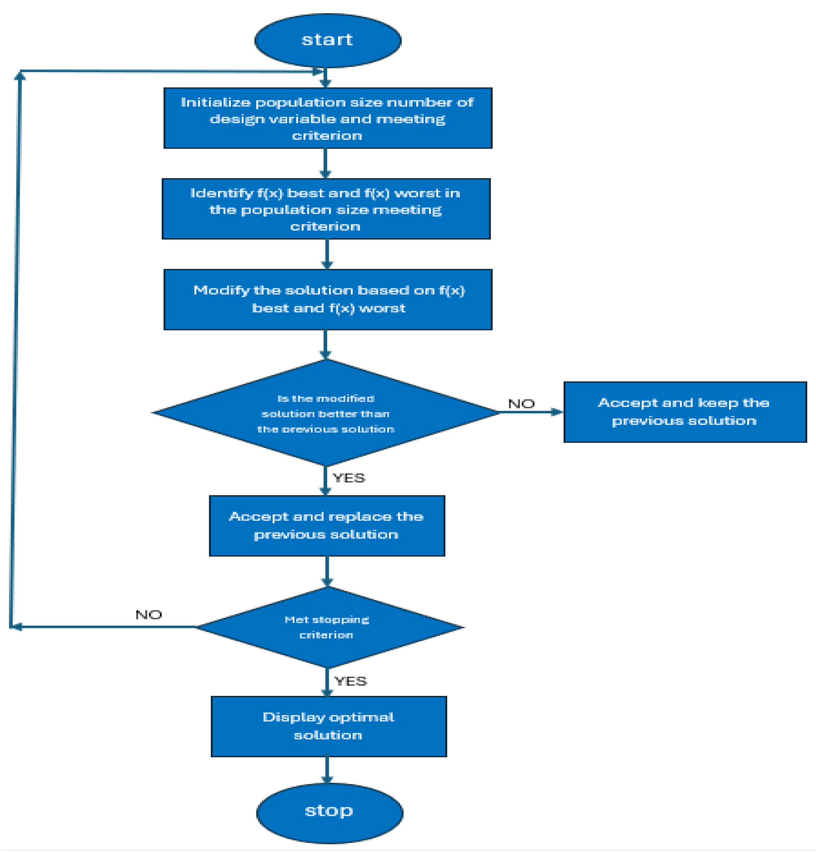
Unlike traditional optimization techniques requiring extensive parameter tuning, JAYA adopts a self-sufficient approach, adjusting solutions dynamically. Once a solution is identified, the algorithm moves closer to the best and steers further from the worst, reinforcing the victory-driven nature of JAYA. Through this iterative refinement, the algorithm consistently strives for efficiency and precision, making it a highly effective optimization strategy.
JAYA Algorithm Implementation
- Initialize the population size (IPZ), design variables, and fitness function evaluation count (FFE).
- Assess the fitness function value for each candidate solution.
- Set FEE = NP (initial evaluation count).
-
While FEE < Max_FEE, repeat the following steps:
- Select the best candidate (xbest) and the worst candidate (xworst) from the population.
- For i = 1 to NP, evaluate the fitness function value for the updated candidate.
- Increment FEE = FEE + 1.
- Accept the new solution only if it outperforms the previous one.
- End iteration once optimal criteria are met.
By continuously refining each candidate’s position, JAYA eliminates reliance on complex parameter tuning, making it an efficient and scalable optimization framework. Whether applied to engineering, data science, or machine learning, its ability to maximize potential while avoiding poor solutions makes it a standout algorithm for robust decision-making
4. Results and Discussion
To evaluate system performance, a controlled indoor simulation environment was designed, replicating real-world conditions within a 4m × 4m × 3m room. Receivers were strategically positioned 1m above the floor, ensuring varied signal propagation pathways.
4.1. Noise and Transmission Sources
Eight Luminous-LED Plyc4545 (PAR38) light-emitting diode lamps were incorporated as noise sources. With a Lambertian order of 33.1 and an emitted power of 65W, these sources exhibited highly directive characteristics, significantly influencing system performance. Their high Lambertian order made them more focused than the diffuse spots, reinforcing their role as interference factors.
Simultaneously, eight diffuse spots, functioning as secondary independent transmitters, were implemented to facilitate signal distribution. These spots played a crucial role in adaptive transmission, ensuring robust signal coverage across the indoor space.
4.2. Optimization Scenarios
To investigate the impact of transmission patterns, two distinct optimization scenarios were considered:
- Scenario P: The eight diffuse spots were uniformly arranged along the perimeter of a 0.5m radius circle, creating a structured and predictable transmission pattern.
- Scenario Q: The eight diffuse spots were randomly distributed within the room, generating a more dynamic and unpredictable transmission environment.
Despite differing placements, the diffuse spot intensities remained non-uniform, with random distributions ensuring varied transmission characteristics. However, total emitted power remained consistent at 2W, standardizing energy output for comparative analysis.
Table 1 provides a comprehensive overview of the key simulation parameters utilized for both PSO and JAYA algorithms, highlighting essential system attributes that guided performance evaluation.
To evaluate system performance, a controlled indoor simulation environment was designed, replicating real-world conditions within a 4m × 4m × 3m room. Receivers were strategically positioned 1m above the floor, ensuring varied signal propagation pathways.
4.3. Noise and Transmission Sources
Eight Luminous-LED Plyc4545 (PAR38) light-emitting diode lamps were incorporated as noise sources. With a Lambertian order of 33.1 and an emitted power of 65W, these sources exhibited highly directive characteristics, significantly influencing system performance. Their high Lambertian order made them more focused than the diffuse spots, reinforcing their role as interference factors.
Simultaneously, eight diffuse spots, functioning as secondary independent transmitters, were implemented to facilitate signal distribution. These spots played a crucial role in adaptive transmission, ensuring robust signal coverage across the indoor space.
4.4. Optimization Scenarios
To investigate the impact of transmission patterns, two distinct optimization scenarios were considered:
- Scenario P: The eight diffuse spots were uniformly arranged along the perimeter of a 0.5m radius circle, creating a structured and predictable transmission pattern.
- Scenario Q: The eight diffuse spots were randomly distributed within the room, generating a more dynamic and unpredictable transmission environment.
Despite differing placements, the diffuse spot intensities remained non-uniform, with random distributions ensuring varied transmission characteristics. However, total emitted power remained consistent at 2W, standardizing energy output for comparative analysis.
F=∑_(k=1)*NR(ω_1×SNR_r-ω_2×DS_k)
The fitness function used for optimization (Equation (8)) considered both delay spread (DSk) and signal-to-noise ratio (SNRk) at each of the NR receivers (Rxs). It is defined as:
where: ω1 = 1 and ω2 = 1 x 10⁹ represent the weights assigned to each component of the fitness function. These weights balance the influence of delay spread and SNR on the overall optimization objective. The large value of ω2 suggests a strong emphasis on maximizing SNR.
Fitness = ω1 * Σ(DSk) + ω2 * Σ(1/SNRk) for k=1 to NR.
4.5. Impact of Delay Spread and Optimized DiS Configurations
Delay spread (DSₖ) is a critical factor in optical wireless communication systems, as it directly influences the achievable bit rate and bandwidth (BW) at the receivers. Excessive DSₖ can lead to intersymbol interference, reducing signal clarity and limiting transmission efficiency. To counteract these effects, DSₖ is strategically incorporated into the fitness function, ensuring the optimization process prioritizes minimal signal dispersion while maximizing overall system performance.
4.6. Optimized DiS Placement and Intensity Distributions
Figure 3a,b illustrate two distinct scenarios for diffuse spot (DiS) placement and intensity allocation, highlighting their impact on receiver signal quality:
- Figure 3a – Circular Arrangement: Rxs 1 and 4 experience the highest susceptibility to noise due to their proximity to multiple noise sources. Conversely, Rxs 2 and 3 are less affected since each is near only one noise source, leading to improved signal reception and reduced interference.
- Figure 3b – Scattered Distribution: The intensity allocation reveals a significant power concentration in DiS 8, which exceeds the output of other DiSs. This is because DiS 8 is tasked with simultaneously serving two receivers (Rxs 1 and 3), with Rx 3 positioned farther away. To ensure reliable signal transmission at greater distances, DiS 8 must emit higher power, compensating for signal attenuation over the propagation path.
4.7. Optimized Diffuse Spot Placement and Performance Analysis
Figure 4 presents results from the second scenario, demonstrating how optimized diffuse spot (DiS) placement enhances system performance. The strategic positioning of DiSs closer to their respective receivers (Rxs) ensures improved signal transmission:
- S2 and S3 align near Rx3, optimizing coverage.
- S1, S6, and S7 cluster around Rx2, reinforcing signal stability.
- S4 and S8 support Rx4, mitigating interference.
- S5 targets Rx1, optimizing transmission efficiency.
Notably, Rx1 and Rx4 are positioned near noise sources, making them more vulnerable to interference.
4.8. Intensity Distribution and Signal Optimization
Figure 4b reveals that S8 exhibits a higher power level than other DiSs. This is because S8 serves Rx4 while simultaneously being close to Rx1, both of which are near noise sources. The increased intensity of S8 compensates for signal degradation, leading to higher signal-to-noise ratio (SNR) values at Rx1 and Rx4. This distribution ensures a more uniform SNR balance across all receivers, stabilizing communication performance.
4.9. Comparative Performance Analysis
Table 2 and Figure 5 provide a detailed comparison of key system metrics, evaluating average SNR, delay spread (DS), standard deviation of SNR, and standard deviation of delay spread across different optimization scenarios:
- Scenario 1 – Initial unoptimized configuration.
- Scenario 2 – Optimized DiS placement for refined signal transmission.
- Scenario X – Centrally positioned DiSs with uniform power distribution.
- Scenario Y – JAYA-optimized DiS distribution for maximum efficiency.
Key Observations from JAYA vs. PSO Optimization:
-
Optimized Center Placement (JAYA vs. PSO):
- ○
- JAYA’s center-based optimization yielded a 23.26% improvement in average SNR and a 28.87% improvement in SNR standard deviation over PSO.
- ○
- Average DS improved by 19.7%, indicating better temporal signal distribution compared to Scenario 1’s unoptimized layout.
- ○
- AYA also demonstrated faster convergence and better delay spread control, though Scenario 1 exhibited slightly better standard deviations for SNR and DS.
-
Optimized Locations & Intensities (Scenario 2):
- ○
- Refining both placement and intensity of randomly distributed DiSs in Scenario 2 led to a 1.76% increase in average SNR and a 12% reduction in average DS relative to Scenario 1.
- ○
- JAYA’s optimization outperformed PSO in DS standard deviation, though reference [8] reported slightly superior DS standard deviation results.
4.10. Impact of Variable Count on Optimization
Scenario 2 introduced 24 adjustable variables, exceeding Scenarios Y (2) and 1 (10), providing greater adaptability in DiS adjustments based on environmental factors. This higher degree of flexibility explains the observed improvements in SNR, DS, and SNR standard deviation.
Figure 4 visually highlights how optimized parameter tuning enhances DiS placement, enabling the system to intelligently adjust transmission characteristics for maximum efficiency and stable performance. Expanding optimization parameters allows greater precision, ensuring optimal wireless communication quality across dynamic indoor environments.

Table 2.
Comparison of the Optimization Scenarios using PSO.
| Optimized Scenarios |
Average Delay Spread (sec) |
STD of DS |
Average SNR (dB) |
STD of SNR |
|
Scenario X (Eltokhey et al., 2019) |
1.0270×10⁻⁹ | 0.8462×10⁻⁹ | 17.9881 | 3.5656 |
|
Scenario Y (Eltokhey et al., 2019) |
0.9528×10⁻⁹ | 0.5833×10⁻⁹ | 19.4327 | 1.1508 |
| Scenario 1 | 0.90296 x 10⁻⁹ | 0.5095 x 10⁻⁹ | 19.8667 | 1.0781 |
| Scenario 2 | 0.85615 x 10⁻⁹ | 0.4880 x 10⁻⁹ | 22.7776 | 0.9974 |
Table 3.
Comparison of the Optimization Scenarios.
| Optimized Scenarios |
Average Delay Spread (sec) |
STD of DS |
Average SNR (dB) |
STD of SNR |
| Scenario 1 | 0.8284 x 10⁻⁹ | 0.395 x 10⁻⁹ | 24.6022 | 0.9422 |
| Scenario 2 | 0.7306 x 10⁻⁹ | 0.3595 x 10⁻⁹ | 25.042 | 0.8990 |
4.11. Analysis of SNR and Delay Spread Across Optimization Scenarios
A comparative evaluation of signal-to-noise ratio (SNR) and delay spread (DS) across multiple scenarios provides key insights into system performance improvements and trade-offs.
4.11.1. Scenario 1 vs. Scenario 2: Performance Trade-Offs
Scenario 1 represents the initial setup, exhibiting solid SNR and delay spread values. However, Scenario 2, which incorporates optimized DiS locations and intensities, demonstrates measurable improvements:
- 1.76% increase in average SNR
- 12% reduction in average DS
Despite these gains, Scenario 2 introduces a higher standard deviation in SNR, reflecting a broader variation across receivers. Applying the Jaya algorithm, the delay spread standard deviation in Scenario 2 outperforms PSO, though it remains slightly worse than reference [8].
4.11.2. Variable Count and System Adaptability
Scenario 2 benefits from an expanded optimization variable set (24) compared to Scenario Y (2) and Scenario 1 (10), allowing greater adaptability in refining the DiS configuration. This increased flexibility enables precise DiS positioning around the receivers (Figure 4), leading to significant improvements in SNR and DS.
4.11.3. Evaluating SNR Stability (Figure 5 - SNR Bar Chart)
Figure 5 visually contrasts the maximum and minimum SNR values across the four scenarios:
- Scenario Y (Jaya optimization) improves minimum and average SNR, reducing the difference between max/min SNR, leading to a more stable SNR standard deviation (Table 2).
- Scenario 1 exhibits higher max, min, and average SNR than Scenario A, but its standard deviation is higher due to greater disparity between max/min SNR values.
- Scenario 2 shows broad improvements in average, min, and max SNR, yet displays a 2.8 dB gap between max/min SNR values. This difference suggests that while average SNR improves, the variation across receivers increases, impacting stability.
4.11.4. Eye Safety Considerations in Real-World Applications
In practical implementations, eye safety regulations must be prioritized when determining maximum transmit power. Factors such as:
- DiS placement,
- Number of transmitters, and
- Lambertian reflection properties,
all play a crucial role in ensuring compliance. While this study focuses on impulse response-based proof-of-concept optimization, real-world deployments must strictly adhere to safety standards, reinforcing operational integrity.
The analysis highlights the benefits and trade-offs of optimization algorithms, emphasizing the role of variable count, adaptability, and DiS placement in improving SNR and delay spread. By refining DiS positioning and intensity, optical wireless systems can enhance communication stability while addressing safety constraints for real-world applications.
4.12. Focus on Signal-to-Noise Ratio (SNR) Optimization
With the DS values successfully meeting the constraints for a maximum bit rate of 100 Mbps, the optimization emphasis now shifts toward SNR, as depicted in Figure 6.
By achieving acceptable DS levels, the system effectively minimizes intersymbol interference, ensuring stable high-speed data transmission. However, SNR remains a crucial determinant of communication reliability, as it directly impacts signal clarity, reception quality, and error rates across the transmission channel.
Figure 6 highlights how refined diffuse spot (DiS) placement and intensity adjustments influence SNR distribution, optimizing overall performance and signal stability. Higher SNR values across receivers translate to improved transmission fidelity, reinforcing the system’s capacity to operate under dynamic indoor conditions.
This strategic focus on SNR enhancement ensures a robust optical wireless communication framework, capable of supporting efficient data transmission, minimizing noise interference, and providing superior overall connectivity.
5. Conclusions
This study explored the optimization of diffuse spot (DiS) placement and intensity in indoor visible light OWC systems, with the primary objective of maximizing SNR and minimizing DS. By analyzing various optimization scenarios, the research assessed how the number of optimization variables impacts SNR and DS performance across different user environments.
Key Findings and Impact
- Significant Performance Gains: The Jaya algorithm demonstrated its effectiveness by achieving up to a 29% improvement in SNR and a 23.3% reduction in delay spread, reinforcing its superiority in signal refinement.
- Enhanced Stability: The optimization process contributed to better standard deviations in SNR (up to 5%) and delay spread (up to 9.9%), ensuring greater consistency in performance despite challenges such as ambient light interference and multipath dispersion.
- Hybridization and Increased Variable Count: The study highlights the advantages of combining optimization algorithms while expanding the number of adjustable variables. This approach enhances the adaptability of diffuse spots, allowing them to dynamically adjust to environmental conditions, ultimately boosting overall system efficiency and communication reliability.
Final Implications
These results affirm the importance of strategic optimization in optical wireless systems, demonstrating how adaptive placement and intensity control can significantly improve SNR stability, delay spread management, and signal transmission quality. Future research could further refine hybrid algorithm approaches to enhance real-time adaptability, ensuring robust high-speed communication in diverse indoor environments.
Author Contributions
Conceptualization, B. Babadoko; methodology, B. Babadoko; software, Mike. David.,Suleiman Zubair.,Abraham U. Usman.,; validation, Mike. David.,Suleiman Zubair.,Abraham U. Usman.,.; Mike. David.,Suleiman Zubair.,Abraham U. Usman.,; investigation, Mike. David.,Suleiman Zubair.,Abraham U. Usman.; Mike. David.,Suleiman Zubair.,Abraham U. Usman.,; data curation, B. Babadoko.; writing—original draft preparation, B. Babadoko.; writing—review and editing, Mike. David.,Suleiman Zubair.,Abraham U. Usman., A. D. Morakinyo., Stephen S. Oyewobi., Topside. E. Mathons,; visualization, Mike. David.,Suleiman Zubair.,Abraham U. Usman., A. D. Morakinyo., Stephen S. Oyewobi.,Topside. E. Mathons,.; supervision, Mike. David.,Suleiman Zubair.; project administration, Mike. David.,Suleiman Zubair.,Abraham U. Usman., A. D. Morakinyo., Stephen S. Oyewobi.,Topside. E. Mathons.; funding acquisition, Mike. David.,Suleiman Zubair.,Abraham U. Usman., A. D. Morakinyo., Stephen S. Oyewobi.,Topside. E. Mathons. All authors have read and agreed to the published version of the manuscript.
Funding
This research was funded by Tshwane University of Technology.
Acknowledgments
We sincerely appreciate the Nigerian Communications Commission (NCC) for their generous sponsorship and steadfast support in making this publication possible. Their dedication to fostering research and innovation through the NCC Endowment Chair at the Federal University of Technology, Minna has been invaluable. Their unwavering commitment to academic excellence and technological advancement continues to shape the future of communication systems and scientific inquiry, empowering researchers to push the boundaries of knowledge. We are deeply grateful for their visionary leadership and investment in advancing education and research
Conflicts of Interest
The authors declare no conflicts of interest. The funders had no role in the design of the study; in the collection, analyses, or interpretation of data; in the writing of the manuscript; or in the decision to publish the results.
References
- Agiwal, M. , Roy, A., & Saxena, N. (2016). Next generation 5G wireless networks: A comprehensive survey. IEEE Communications Surveys & Tutorials, 18(3), 1617-1655. [CrossRef]
- Alsulami, O. , Hussein, A. T., Alresheedi, M. T., & Elmirghani, J. M. H. (2018). Optical wireless communication systems: A survey. IEEE Transactions on Communications. [CrossRef]
- Arfaoui, M. A. , Soltani, M. D., Tavakkolnia, I., & Ghrayeb, A. (2020). Measurements-based channel models for indoor LiFi systems. IEEE Access. [CrossRef]
- Chowdhury, M. Z. , & Hasan, M. K. (2019). The role of optical wireless communication technologies in 5G/6G and IoT solutions. IEEE Transactions on Wireless Communications. [CrossRef]
- Javaid, F. , et al. (2021). Characteristic study of visible light communication and influence of coal dust particles in underground coal mines. Optical Wireless Communication Journal. [CrossRef]
- Khalighi, M. A., et al. (2021). Optical wireless communications for emerging connectivity requirements. IEEE Open Journal of the Communications Society, 2, 82–86. [CrossRef]
- Kirrbach, R. , Faulwaßer, M., Jakob, B., Schneider, T., & Noack, A. (2019). Li-Fi for augmented reality glasses: A proof of concept. In 2019 IEEE International Symposium on Mixed and Augmented Reality Adjunct (ISMAR-Adjunct) (pp. 263-268). IEEE. [CrossRef]
- Lebaka, M. (2006). Optimization of spot pattern in indoor diffused optical wireless systems. IEEE Photonics Technology Letters. [CrossRef]
- Manousiadis, P. , et al. (2020). Organic semiconductors for visible light communications. Journal of Photonic Research. [CrossRef]
- Stassen, M. , & Colak, S. B. (2020). Infrared communication channel optimization for quasi-diffuse multi-spot wireless indoor networking. IEEE Transactions on Wireless Communications.
- Switching, Optical. (2019). Optimization of intensities and locations of diffuse spots in indoor optical wireless communications. IEEE Transactions on Wireless Communications. [CrossRef]
- Wong, D. W. K. , & Chen, G. C. K. (2005). Optimization of spot pattern in indoor diffuse optical wireless local area networks. IEEE Journal of Selected Areas in Communications.
- Wu, D. , et al. (2020). Hybrid LiFi and WiFi networks: A survey. IEEE Transactions on Wireless Communications. [CrossRef]
- Chen, X., Li, C., Chen, L., Wang, H., Zang, Y., & Yao, W. (2020). Influence of different structure and specification parameters on the propagation characteristics of optical signals generated by GIL partial discharge. Energies, 13(12), 3241. [CrossRef]
Figure 1.
Showing the indoor OWC environment considered in this work.
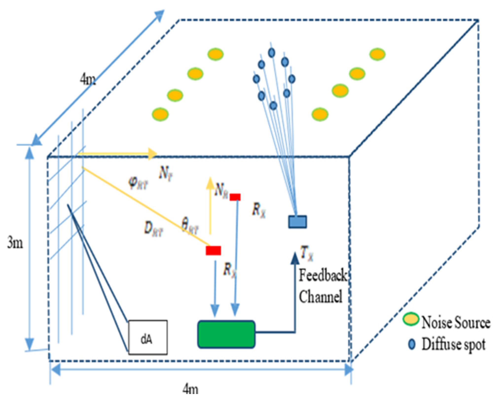
Figure 3.
Showing the indoor OWC environment considered in this work.
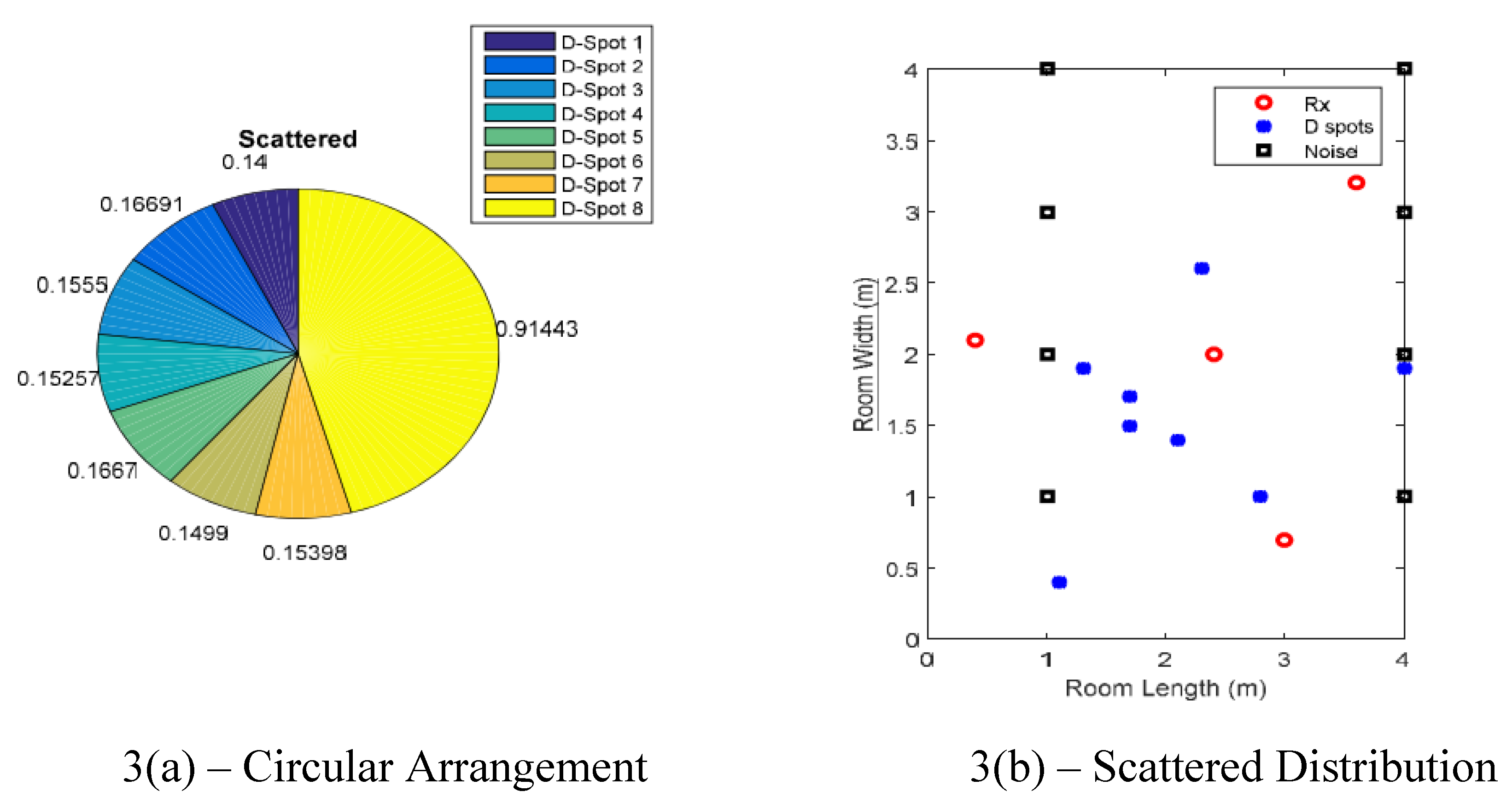
Figure 4.
Optimized parameter for the diffuse spot of the First Scenario (i.e., circular) from the top.
Figure 4.
Optimized parameter for the diffuse spot of the First Scenario (i.e., circular) from the top.
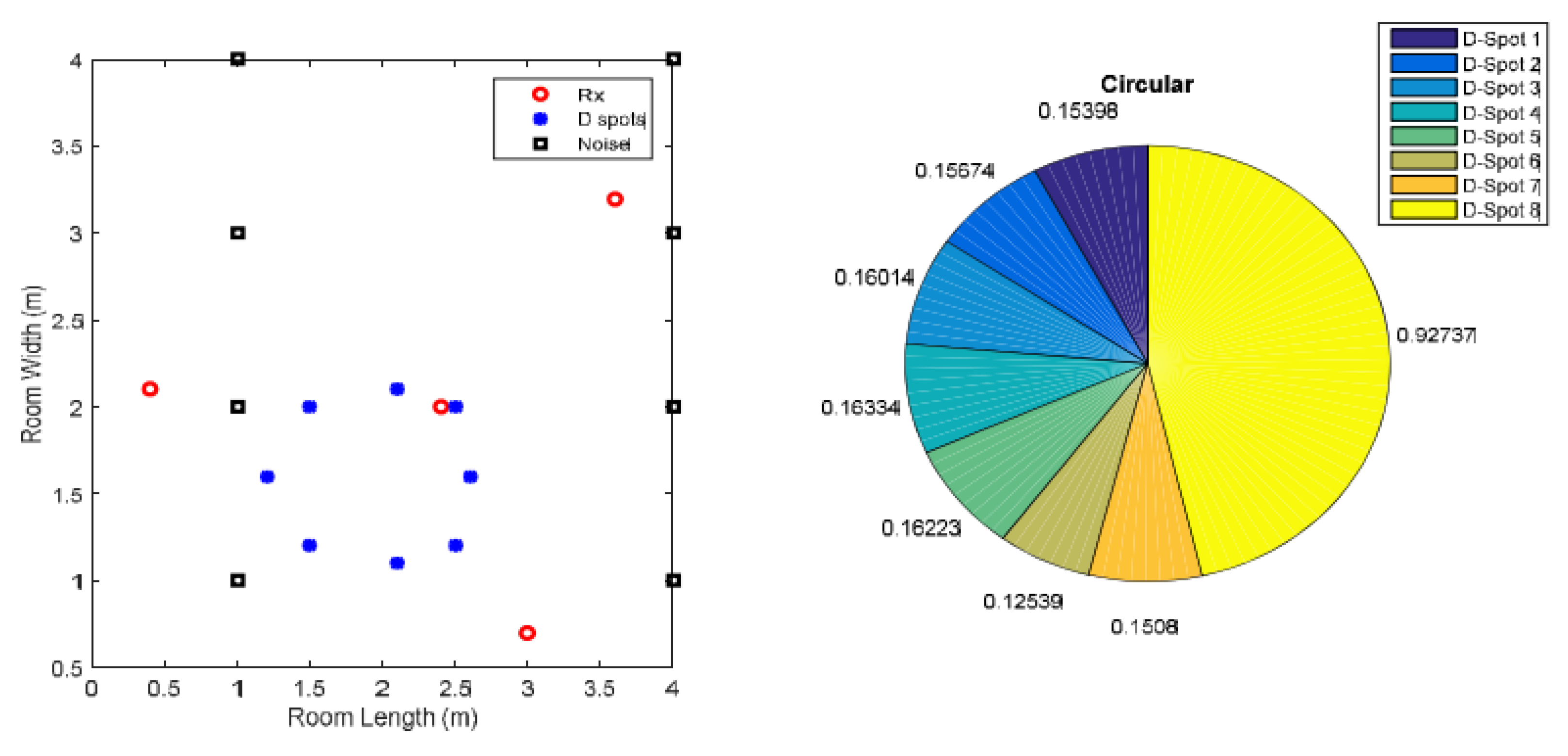
Figure 5.
Minimum and Maximum SNR obtained.
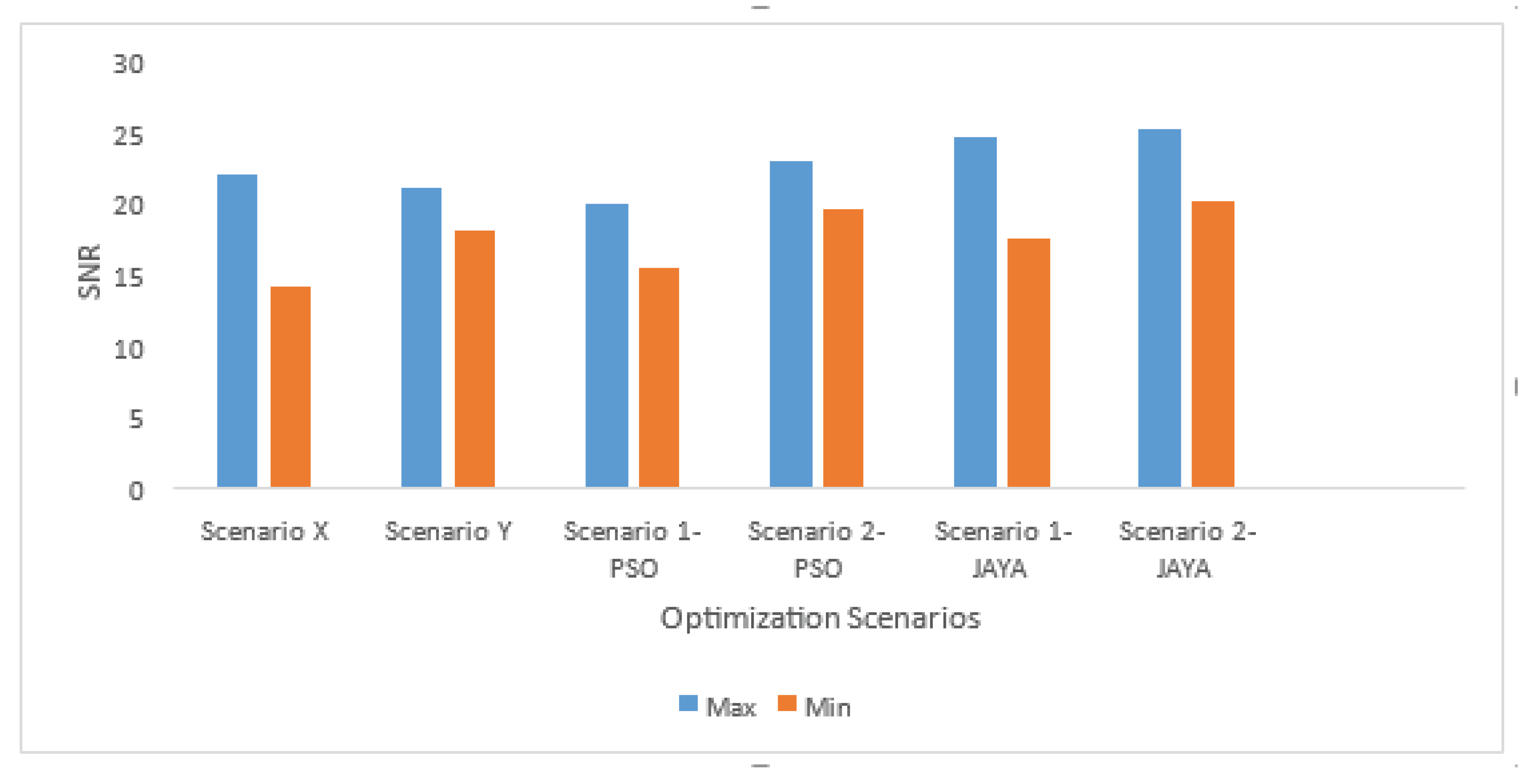
Table 1.
Simulation Parameter.
| S/No | Parameter | Values |
|---|---|---|
| 1 |
PSO Algorithm Nos of Iteration Nos of Particles Nos of Evaluations |
100 50 5000 |
| 2 |
Jaya Algorithm population size, N Dimension, D |
100 4 |
| Room dimension | 4 x 4 x 3 | |
| Reflectivity of the wall | 0.8 | |
| Reflectivity of the ceiling | 0.8 | |
| Reflectivity of the wall | 0.3 | |
| Receivers locations | (1.6,2.1,1), (4.8,4.5.1), (3.3,0.7,1), (0.4,2.2,1) | |
| Noise source location | (1.1.3), (1,2,3), (1,3,3), (1,4,3), (4,1,3), (4,2,3), (4,3,3), (4,4,3) | |
| Photodetector (PIN) responsivity | 0.5 A/W | |
| Bit rate | 100Mbps | |
| Receiver bandwidth | 70Mhz |
Disclaimer/Publisher’s Note: The statements, opinions and data contained in all publications are solely those of the individual author(s) and contributor(s) and not of MDPI and/or the editor(s). MDPI and/or the editor(s) disclaim responsibility for any injury to people or property resulting from any ideas, methods, instructions or products referred to in the content. |
© 2025 by the authors. Licensee MDPI, Basel, Switzerland. This article is an open access article distributed under the terms and conditions of the Creative Commons Attribution (CC BY) license (http://creativecommons.org/licenses/by/4.0/).
Copyright: This open access article is published under a Creative Commons CC BY 4.0 license, which permit the free download, distribution, and reuse, provided that the author and preprint are cited in any reuse.


