Submitted:
10 September 2025
Posted:
11 September 2025
You are already at the latest version
Abstract
We aimed to understand and explore the intracultivar variability of soybean lines by conducting both phenotypic and genotypic analyses. During the 2017/2018 crop sea-son, plants from six soybean cultivars (SYN1359S IPRO, P98Y11, BMX6160, 97R73 RR, NS7000 IPRO, and NA5909) were used to set the genetic treatments. For each of these six cultivars, 47 plants were pulled to generate progenies and, along with the controls, were subjected to trials across two subsequent crop seasons, 2018/2019 and 2019/2020. Phenotypic traits such as Grain Yield (YIELD), Full Maturity (FM), Days to Flowering (DF), and Plant Height (PH) were measured. Additionally, 288 samples (progenies and controls) were genotyped by a chip with 1329 SNPs using the Ion S5™ XL System. Phenotypic data were analyzed using mixed models. The genotypic analysis included measures such as observed and expected heterozygosity, hierarchical clustering (UP-GMA), and principal component analysis (PCA). The study reveals the existence of both phenotypic and genotypic intracultivar variation among the assessed cultivars. The degree of variation observed differs, with cultivars P98Y11 and NA5909 exhibiting higher levels of diversity, while NS7000 presents a lower level of variation. This re-flects the fact that the genome is not static but rather dynamic, constantly subject to genetic and environmental influences that shape diversity.
Keywords:
Glycine max L. Merrill.
; plant breeding
; genetic diversity
; genetic stability
1. Introduction
Pure line selection isolates the best genotypes from a heterogeneous population by selecting individual plants and evaluating their progenies. In this process, no new genotype is created, as the goal is simply to identify and preserve superior genotypes within the existing population [1]. This breeding strategy has been studied in different crops, such as bean [2], wheat [3], soybean [4] and rice [5].
Selection of pure and homozygous lines is a fundamental goal of plant breeding programs. Soybean lines are typically developed to be used as a cultivar. Nonetheless, the genetic stability of these lines is prone to intra-cultivar variation, which can manifest as genomic changes and structural alterations over time [6].
Several mechanisms, including residual heterozygosity, mutations, transposable elements, epigenetic modifications, process of cross-pollination and chromosomal mutations [6], can induce genomic changes which contributes to phenotypic variability within cultivars. These genomic alterations may impact the stability of lines over time but can also present opportunities for breeding programs.
The development of new soybean cultivars requires significant investment, and the evaluation and selection of superior plants within existing cultivars is considered a cost-effective breeding strategy. The selection within a soybean cultivar raises important considerations in the context of plant variety protection, which is essential for intellectual property rights and the encouragement of breeding programs [7]. In this way, we aimed to investigate the intracultivar variability of soybean lines through phenotypic and genotypic data, as well as to understand the genetic stability and genomic dynamic in soybean cultivars.
2. Materials and Methods
2.1. Plant Material and Field Trials
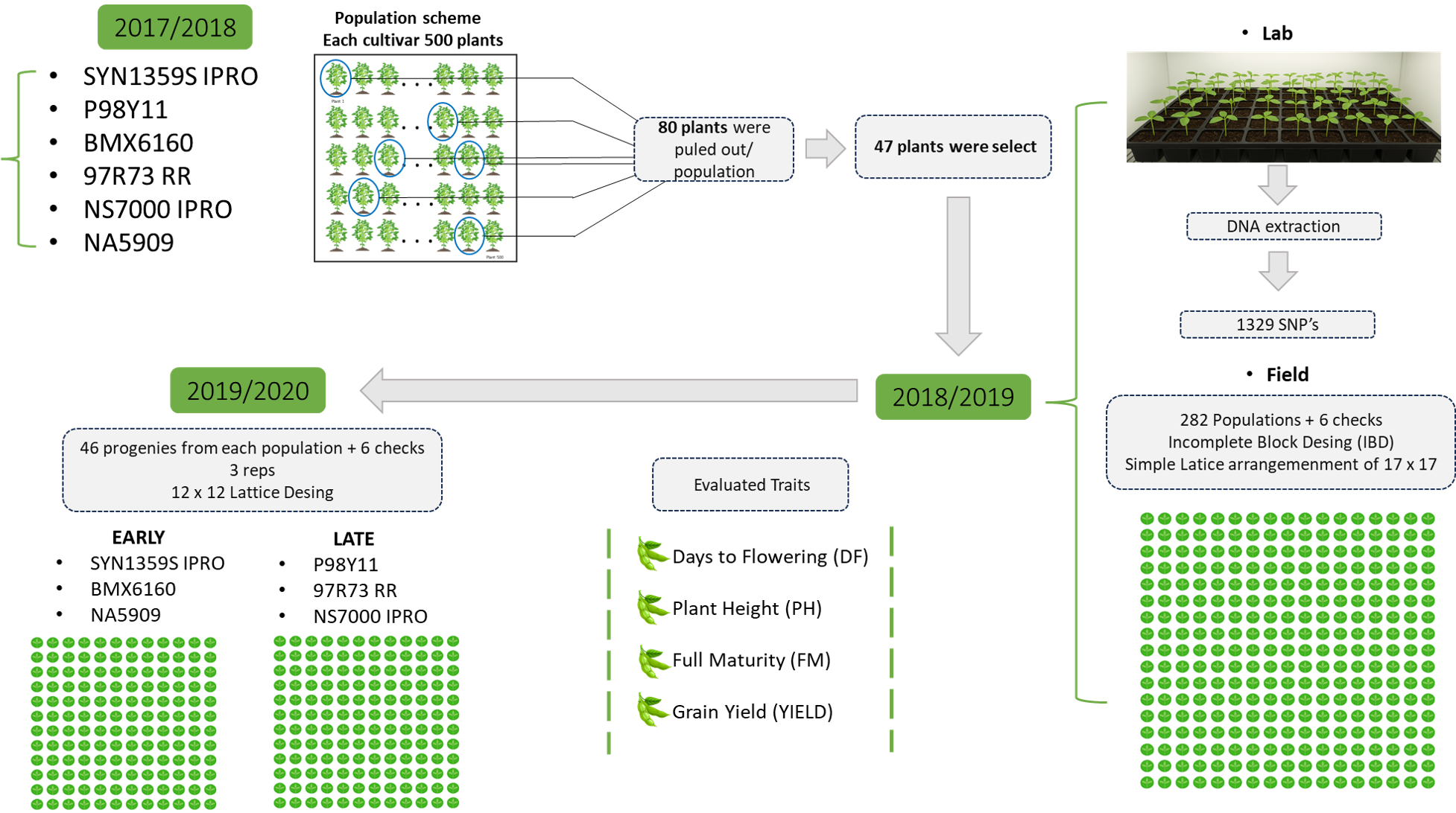
The experiments were carried out at the Muquém Farm, from Federal University of Lavras (UFLA) (21°14' S; 45°00' W), Lavras- MG, Brazil, in the 2017/2018 crop season, with the selection of plants from the SYN1359S IPRO, P98Y11, BMX6160, 97R73 RR, NS7000 IPRO, and NA5909 cultivars. Each cultivar was growed in a population scheme consisting of 500 plants per cultivar. From each population, 80 plants were pulled. Out of these 80 plants, a total of 47 were selected to progenies trials. These progenies were then evaluated alongside control samples across two cropping seasons, 2018/2019 and 2019/2020.
2.2. Experimental Design
The experiment was carried out in 2018/2019 cropping season utilized an incomplete block design (IBD), specifically a simple lattice arrangement of 17x17, resulting in 288 treatments. These treatments included 282 progenies, in addition to 6 control varieties, which were SYN1359S IPRO, P98Y11, BMX6160, 97R73 RR, NS7000 IPRO and NA5909. The experimental plots were set up as single rows, 2 m lenght and 0.5 m apart.
In the 2019/20 crop season, the progenies were split into two experiments based on their maturity group: early and late. The early experiment included 46 progenies from each of the early-maturing cultivars (SYN1359S IPRO, BMX6160, and NA5909), as well as the six control cultivars. The late experiment comprised 46 progenies from each of the late-maturing cultivars (NS7000, P98Y11, and 97R73), along with the same six control cultivars. Both experiments were conducted with three replications in a 12x12 lattice design. Each experimental plot consisted of two rows, with two meters in length and 0.5 m apart.
The following traits were assessed: (1) Grain Yield (YIELD): was quantified as the amount harvested from each plot and expressed in kg ha−1 at a 13% moisture content; (2) Days to Flowering (DF): was the number of days from sowing to the R2 stage, at which point 50% of the plants exhibit full flowering; (3) Full Maturity (FM): was the number of days from sowing until the R8 stage (full maturity) is reached, defined as the point when 90% of the plants in the plot have attained this stage, according to the criteria set by Fehr and Caviness (1977) and (4) Plant Height (PH): was measured in cm from the base of the plant to the insertion point of the uppermost leaf at harvest. Three plants were randomly selected from each plot for measurement.
2.3. Phenotypic Data analysis
Data were analyzed adopting a mixed-model approach. The experiments from each year, categorized by relative maturity groups, were individually analyzed using model one.
where : Observed value for the analyzed trait, : constant associated with all observations, : vector of replicate fixed effect, : vector of checks or test fixed effect, : vector of progenies effect (random), , : vector of block effect aligned with replications (random), , : vector of population effects the six cultivars (random), and : vector of associated error effect (random), .
Residual normality was assessed using the Shapiro-Wilk test [8], and homogeneity of variances across the experiments was evaluated using Hartley's maximum F test [9]. The joint analysis of environments was performed using model two.
where: : Observed value for the analyzed trait, : constant associated with all observations, : vector of replicate fixed effect, : vector of maturity group fixed effect, : vector of checks or test fixed effect, : vector of population effects the six cultivars (random), , : vector of environment effects the years (random), , : vector of progenies effect (random), , : vector of interaction effect progenies × environment (random), , : vector of block effect aligned with replications (random) , and : vector of effect of associated errors (random), .
The matrix of residual variances and covariances was configured with a diagonal structure as a response to identified heterogeneity within the dataset. The next phase involved modeling the variance and covariance matrix for the genotype-by-environment interaction. For this purpose, an extended form of the factor analytic (FA) structure was applied, guided by the Bayesian Information Criterion (BIC) and the Akaike Information Criterion (AIC) to determine the most suitable model.
Progeny, population and total heritability were estimated. Accuracy was calculated at three levels: population, progeny, and overall accuracy. Additionally, the coefficient of variation of the experimental error was determined for each evaluated variable to assess the precision and consistency of the data.
2.4. DNA Extraction, Library Preparation, and Sequencing
The seeds of the 288 genotypes were sown in trays and placed in a growth chamber maintained at 25°C. The seeds were grown until the emergence of the first trifoliate and six leaf punches were collected from each genotype. The samples were immediately frozen and stored at -80°C, subsequently, the samples were lyophilized (freeze-dried) to remove moisture.
DNA extraction and genotyping were conducted using the KLEARGENE commercial kit. A Chip for sequencing was used to target 1329 single nucleotide polymorphism (SNP) markers for genotyping. Sequencing was performed on the ION S5 sequencer from Thermo Fisher Scientific.
The amplification reaction included the AgriSeq Amplification Mix, Ion AmpliSeq™ Primer Pool specific to the SNPs of interest, and nuclease-free water to avoid any contamination from DNases or RNases. The thermocycling process for amplification involved several steps: enzyme activation, DNA strand denaturation, primer annealing, and DNA synthesis. Next, unique adapters or barcodes were ligated to the amplified DNA fragments to identify each sample uniquely. This step involved the addition of a Barcode Reaction Mix and another round of thermocycling.
After adapters bind, the library was normalized to ensure sequencing coverage across samples and a purification step was done to remove any non-amplified fragments. The purified and normalized libraries was prepared for loading into the ION CHEF system, which automates template preparation and chip loading for the ION S5 sequencer.
The final step was sequencing those libraries on the Ion S5™ XL System, which can deliver up to 80 million reads per run. Bioinformatic analysis was then performed using Torrent Suite™ Software, which processed the sequencing data on a computer connected to the Ion Torrent™ server. The outcome of this analysis was a matrix, listing the genotypes alongside their corresponding SNP markers.
2.5. Selection, Imputation, and Coverage of SNPs
Monomorphic SNPs and those with a Minor Allele Frequency below 5% were removed. Genotypes with a call rate below 75% were excluded. The final dataset comprised 605 selected SNPs and 267 genotypes. For the imputation of missing data, the LD-kNNi algorithm was used [10]. After filtering and imputation, SNPs were distributed across 20 soybean chromosomes (Figure 1), with positions shown equidistantly, not reflecting actual chromosome size.
2.6. Population Analyses
Genetic diversity was estimated using expected heterozygosity (He) and observed heterozygosity (Ho) across loci. The genetic distance between populations was calculated using the Prevosti (1975) [11] method and the resulting distance matrix was employe in a hierarchical clustering analysis using the unweighted pair group method with arithmetic mean (UPGMA). The starting point for the clustering was the smallest distance and this method was chosen due its cophenetic correlation, estimated by the Mantel test with 10,000 permutations to construct a dendrogram.
The Mantel test was used to assess the fit between the hierarchical clustering and the original dissimilarity matrix. After clustering, the cutoff point for group formation was determined using the Mojena method.
To evaluate the genetic relationships among soybean lines and the variation within populations, a pairwise distance matrix was calculated using the Pairwise method [12]. The resulting genetic distance matrix was then used to conduct a principal component analysis (PCA) to visualize the genetic variation. The PCA was plotted on a Cartesian plane, considering the first two principal components, where the specific explanatory capacity was determined by the eigenvalues. Confidence ellipses were added to the PCA plot, assuming a multivariate t-distribution at a 0.05 probability level.
3. Results
3.1. Phenotypic Data
For individual analysis (data not show), results were divided by cycle: early and late-maturity. In early-maturity cultivars, significant differences were observed for YIELD and FM in the 2018/19 season across tests, progenies, populations, and among early populations. In 2019/20, YIELD showed significant variation within tests, populations, and notably within SYN1359. Plant height differed significantly among NA5909 progenies, while DF differences were exclusive to NA5909. For late-maturity cultivars, in 2018/19, YIELD showed significant differences within tests, progenies, populations, and among late populations. In 2019/20, all traits differed significantly within the variety 97R73 and at the progeny level. Additionally, 98Y11 showed significant differences for YIELD and plant height.
Progeny selection accuracy ranged from medium to high, with YIELD accuracy varying from 0.35 (EARLY 19/20) to 0.82 (LATE 18/19). Population selection accuracy (), which measures the accuracy of selection at the population level, exhibited high magnitudes, with values ranging from 0.71 to 0.51 (data not show). These estimates for the variables, in general were higher for the late-maturity group in both years. The estimates of CVe ranged from 1.13 for FM, (LATE 19/20) to 17.91 for YIELD, (EARLY 18/19). The CVgprog is relatively low compared to CVgpop, suggesting more variation among populations than within for most of the traits.
In the multi-environment analysis (Table 1), a significant variation was detected for progenies for the traits YIELD, PH, and FM. Variation was detected among populations for all traits, as well as between early and late maturity cultivars. The variation among progenies within each population was significant for all traits for the late maturity cultivars 97R73 and NS7000. For the cultivars 98Y11, NA5909 and BMX6160, the variation was detected for PH, FM and DF. In addition, for SYN1359, the variation was detected for all traits except for PH.
The environmental variance ( ) was not significant for YIELD and PH, but was significant for FM and DF. In contrast, the interaction () was significant for YIELD, FM and DF, whereas it was not significant for PH.
The progeny heritability ( ), ranged from low, FM (0.12) and YIELD (0.17), to medium, DF (0.45) to high, PH (0.86), nonetheless the population heritability () ranged from low, YIELD (0.18) to high, PH (0.96), FM (0.86) and DF (0.96), in this regard at population level all the traits showed higher heritability. These results followed the same pattern for accuracy, where total accuracy ( ) ranged from medium, YIELD (0.55) to high, PH (0.99), FM (0.94) and DF (0.99).
3.2. Genetic Diversity and Population Structure
UPGMA clustering of the 267 progenies revealed close genetic relationships among cultivars due to shared ancestry (Figure 2). The cophenetic correlation coefficient was 0.92 and significant (Mantel test), indicating that the dendrogram accurately represents the genetic distances among progenies, with minimal distortion introduced by the clustering method.
The first two principal components accounted for 47.11% of the total genetic variability (Figure 3). The analysis revealed six major clusters corresponding to the origins of the progenies from previous cultivars.
The results on Table 2, showed the genetic variation among soybean progenies, these findings are consistent with the PCA results. Cultivars P98Y11 and NA5909, with high He and Ho values, indicating a broad genetic base and potential for intracultivar selection. In contrast, NS7000 showed the lowest diversity (He = 0.047725; Ho = 0.032058), also reflected in its low dispersion in the PCA.
4. Discussion
4.1. Phenotypic Data
Phenotypic variation within cultivars has been reported in soybean ([4]; [7];[13];[6]) and other crops such as potato, wheat, cotton, and barley ([14]; [15]; [16]). This phenotypic variability, even within cultivars, highlights the importance of understanding the genetic basis of traits to improve selection strategies.
Consistent with this premise, the evaluation of late maturing cultivars in both 2018/19 and 2019/20 revealed significant differences not only among cultivars but also within them. In 2018/19, yield differed significantly across the test, progenies, and populations, as well as between the three late maturity cultivars. In 2019/20, this pattern was reinforced, with significant differences detected for all traits within the cultivar 97R73, and at the progeny level for all evaluated traits.
Ninou et al. (2022) [15] found significant variation within improved commercial cultivars of durum wheat for grain yield and protein content. Similarly, significant intracultivar differences over two years and among three locations were observed for cotton yield. The same study also identified intracultivar variation for fiber quality traits such as length and micronaire, while fiber strength and uniformity showed no significant variation. Physiological traits like leaf carbon isotope discrimination, ash content, and potassium concentration also exhibited intracultivar variation [16].
Heritability is a measure of the proportion of variation in a trait that can be attributed to genetic differences among individuals, as opposed to environmental factors. In the multi-environment analysis, the highest values of heritability and accuracy were observed for PH, suggesting that this trait is likely controlled by a small number of genes and the selection for this trait could be effective at the progeny level.
In contrast, the coefficient of variation due to environmental effects (CVe) was very low for FM and DF, showing the greatest precision for this trait (Table 1). Low heritability was observed for YIELD, as expected, due to its high sensitivity to genotype-by-environment (G × E) interactions, which is consistent with the findings of Mendonça et al. (2020) [17].
The lower heritability for YIELD (0,17) and FM (0,12) at progeny level, in the multi-environment analysis, indicates that these traits are strongly influenced by environment. Nonetheless, the detection of significant genotypic variance for both traits demonstrate the presence of exploitable genetic variability. The relatively low coefficients of variation (3.49 for YIELD and 0.43 for FM) further support the precision of phenotypic assessments, reinforcing the reliability of these findings.
Soybean maturity is a complex trait controlled by the interaction of numerous genes, molecular pathways, and the cultivation environment, in the study of Zimmer et al. (2021) [18], several QTL’s associated with maturity groups were identified across different chromosomes, including loci with effects spanning multiple maturity groups.
Similarly, soybean seed yield is also a complex quantitative trait governed by multiple genes and broadly influenced by growing conditions and latitudinal adaptation [19]. The complexity of both traits explains the low heritability, as their phenotypic expression results from intricate gene–environment interactions.
Besides the trait itself, the genetic structure of a population is also crucial in heritability estimation. In self-pollinated plants, we often see high heritability within a population due to homozygosity at many loci, reducing genetic variation for certain traits and making the individuals more genetically similar to each other [20]. This higher heritability within a population is present in Table 1.
The investigation of intracultivar variation in soybeans has disclose several key insights that have implications for soybean breeding and cultivation. The potential for selection within a cultivar stands out as a promising avenue for enhancing desirable traits while maintaining the overall genetic elite background of the cultivar. This potential for selection within a soybean cultivar also raises important considerations in the context of plant variety protection. To qualify for protection under plant variety protection laws, a new cultivar must typically meet the criteria of Distinctness, Uniformity, and Stability (DUS).
Another perspective that emerges when considering intracultivar variation is the multiline cultivars. This strategy aims to enhance yield stability and bolster resilience against both biotic and abiotic stresses. For several soybean breeding programs, the bulk method is commonly employed to manage segregating populations through to the F3 or F4 generations. This approach is also used during the evaluation of progenies within families. As a result, the cultivars that are developed under these conditions are, in essence, a composite of multiple lines rather than a single, pure line [6]. Studies using multiline approach has demonstrated that such cultivars are markedly stable [21] and effective in reducing the severety of asian soybean rust (ASR) [22].
4.2. Molecular Data
Several studies have demonstrated intracultivar variation using molecular tools. Yates et al. (2012) [23] used SSR markers to analyze three soybean cultivars and confirmed heterogeneity in protein and oil content, as well as in fatty acid composition, as previously reported by Fasoula and Boerma (2005) [13]. The majority of intracultivar SSR variation was attributed to residual heterozygosity, resulting in allele polymorphism. Additionally, Achard et al. (2020) [7] employed SNP markers to assess intracultivar variation in a study involving 36 cultivars and 5,346 SNPs, revealing heterogeneity levels ranging from 0 to 10%.
Mihelich et al. (2020) [24] conducted a heterogeneity analysis of 20.087 Glycine max and Glycine soja accessions from the USDA Soybean Germplasm Collection (SGC). The study identified high probability intervals of heterogeneity in 4% of the collection, corresponding to 870 accessions. However, the 'Williams 82' soybean accession showed no evidence of heterogeneity, in contrast to the within 'Williams 82' variation reported by Haun et al. (2011) [25]. The researchers proposed three explanations for the absence of intra-accession variation in 'Williams 82': 1. a genetic bottleneck causing a specific population homogeneity distinct from other varieties; 2. the genotyping sampling was based on three bulks of individuals and might have inadvertently included individuals with identical genotypes; and 3. the 'Williams 82' sample was derived from a single individual, which may not be representative of the accession's potential diversity. This lack of heterogeneity in 'Williams 82' suggests that similar processes could have also obscured the true genetic diversity in other accessions within the SGC.
In this study, genotypic variation is consistent with phenotypic variation. Progeny derived from P98Y11 and NA5909 exhibited significant variations for PH, FM, and DF in multi-environment analysis. So, a considerable genetic diversity was found for a within P98Y11 and NA5909 population analysis, indicating substantial genetic diversity in these populations. Furthermore, at an individual level, they displayed considerable variation for yield and plant height.
Cultivars 97R73 and P98Y11 were grouped together because they both originated from the same breeding company (Corteva - Pioneer). Even though they have different maturity groups, the genetic background could be similar. In contrast, the cultivars NA5909 and NS7000 IPRO exhibit differences, and despite both originating from the same breeding company (Syngenta - Nidera), this variation may be due to the cultivars being derived from different relative maturity groups (RMGs). These findings agree with those reported by Mendonça et al. (2022) [26], indicating that varieties from the same breeding company, particularly those from identical RMGs, have substantial genetic similarity.
The PCA analyses, revealed six major clusters corresponding to the origins of the progenies from previous cultivars. A distinct separation of cultivars 97R73 and P98Y11 from the others corroborates with the dendrogram findings. Notably, the PCA provided a visualization of the high level of variation within the P98Y11 and NA5909 populations, as evidenced by the larger ellipses representing these groups. Conversely, the progenies derived from NS7000 exhibited the smallest variation. This intra-cultivar variation for P98Y11 and NA5909 can be explained by various mechanisms such as residual heterozygosity, mutations, transposable elements, epigenetic modifications, non-homologous recombination, and chromosomal mutations [6].
The genetic variation among soybean progenies derived from six cultivars was assessed by calculating expected heterozygosity (He) values for each population. These He values ranged from 0.047725 in NS7000 to 0.124485 in P98Y11. Additionally, observed heterozygosity (Ho) values were determined for each population to assess the genetic variation within the soybean progenies. The Ho values varied from 0.032058 in NS7000 to 0.112448 in P98Y11, as shown in (Table 2). These findings are consistent with the PCA results, which indicated significant variation in cultivars P98Y11 and NA5909, as reflected by high He and Ho values, indicating a broad genetic base, which suggests potential for intracultivar selection. Conversely, the NS7000 population exhibited the lowest genetic diversity with an He value of 0.047725 and an Ho value of 0.032058 also evidenced by the low dispersion of data points in the PCA. This suggests a more uniform genetic structure within this population [27].
Remaining heterozygosity (HR) has been identified as an important source of intracultivar variation. In bulk breeding, segregating populations are advanced through successive generations of selfing, with the expectation that heterozygosity will be reduced by half each cycle until reaching near fixation. However, studies have shown that natural selection may preserve heterozygous loci when they confer adaptive advantages, as observed by Hockett et al. (1983) [28] even in advanced generations. This indicates that, despite the inbreeding process inherent to the bulk method, HR can persist within families and contribute to phenotypic variability, which may be exploited during selection in later generations.
A study carried out by Fasoula, Yates, and Boerma (2012) [13] using SSR markers in soybean cultivars found 82% to 93% variation attributable to HR. However, even in 100% homogeneous lines, variation can be found, resulted from mutation, intragenic recombination, unequal crossing over, DNA methylation, excision or insertion of transposable elements, and gene duplication ([29]; [30]; [31]).
Another hypothesis is that the genome is dynamic and that new genotypic and phenotypic variation arises in each generation. One source of variation is genetic change leading to alleles with modified effects, that is, de novo generated variation. A second, complementary source of variation could come from interaction or epistatic effects, involving both de novo diversity and the original genetic diversity [32] Given that phenotypic and genotypic variations have been observed across all populations, selection can be employed for soybean breeding.
5. Conclusions
This study reveals the existence of both phenotypic and genotypic intracultivar variation among the assessed soybean cultivars. The degree of variation observed differs, with cultivars P98Y11 and NA5909 exhibiting higher levels of diversity, while NS7000 presents a lower level of variation. This reflects the fact that the genome is not static but rather dynamic, constantly subject to genetic and environmental influences that shape diversity, in addition these results strongly demonstrated that intra-cultivar variations could be explored in soybean plant breeding programs as a breeding tool.
Author Contributions
Conceptualization, E.L.R and A.T.B.; methodology, E.L.R, A.T.B., M.R.P.; software, M.R.P. and D.A.O.; validation, E.L.R., A.T.B., M.R.P. and D.A.O.; formal analysis, M.R.P. and D.A.O.; investigation, E.L.R., A.T.B., B.S.P., M.R.P., D.A.O., V.A.P.S., T.T.T.R.,A.G.S.G.S., C.H.S.; resources, A.T.B.; data curation, E.L.R., A.T.B., B.S.P., M.R.P., D.A.O., V.A.P.S., T.T.T.R.,A.G.S.G.S., C.H.S.; writing—original draft preparation, E.L.R; writing—review and editing, B.S.P. and A.T.B.; visualization, M.R.P. and D.A.O.; supervision, E.L.R.; project administration, E.L.R.; funding acquisition, A.T.B. All authors have read and agreed to the published version of the manuscript.
Acknowledgments
The authors thank the National Council for Scientific and Technological Development (Conselho Nacional de Desenvolvimento Científico e Tecnológico - CNPq) and the Minas Gerais State Agency for Research and Development (Fundação de Amparo à Pesquisa do Estado de Minas Gerais - FAPEMIG) for their support, and the Brazilian Federal Agency for Support and Evaluation of Graduate Education (Coordenação de Aperfeiçoamento de Pessoal de Nível Superior - CAPES). The authors acknowledge the support of the Brazilian National Council for Scientific and Technological Development (CNPq) research productivity scholarship. The authors thank the GDM Genetica do Brasil S. A. for their support.
Conflicts of Interest
The authors declare no conflicts of interest.
References
- Reynolds, M.P.; Braun, H.-J. (Eds.). Wheat Improvement: Food Security in a Changing Climate; Springer: Cham, Switzerland 2022. [CrossRef]
- Santos, P.S.J.; Abreu, A.F.B.; Ramalho, M.A.P. Seleção de linhas puras no feijão ‘carioca’. Ciência e Agrotecnologia 2002, 20, 1492–1498. [Google Scholar]
- Agorastos, A.G.; Goulas, C.K. Line selection for exploiting durum wheat (T. turgidum L. var. durum) local landraces in modern variety development program. Euphytica 2005, 146, 117–124. [Google Scholar] [CrossRef]
- Amaral, L. de O.; et al. Pure line selection in a heterogeneous soybean cultivar. Crop Breeding and Applied Biotechnology. 2019, 19, 277–284.
- Roy, P.S.; Patnaik, A.; Rao, G.J.N.; Patnaik, S.S.C.; Chaudhury, S.S.; Sharma, S.G. Participatory and molecular marker assisted pure line selection for refinement of three premium rice landraces of Koraput, India. Agroecology and Sustainable Food Systems 2016, 41, 167–185. [Google Scholar] [CrossRef]
- Tokatlidis, I.S. Conservation breeding of elite cultivars. Crop Science 2015, 55, 2417–2434. [Google Scholar] [CrossRef]
- Achard, F.; et al. Single nucleotide polymorphisms facilitate distinctness-uniformity-stability testing of soybean cultivars for plant variety protection. Crop Science 2020, 60, 2280–2303. [Google Scholar] [CrossRef]
- Shapiro, S.S.; Wilk, M.B. An analysis of variance test for normality (complete samples). Biometrika 1965, 52, 591–611. [Google Scholar] [CrossRef]
- Hartley, H.O.J.B. The maximum F-ratio as a short-cut test for heterogeneity of variance. Biometrika 1950, 37, 308–312. [Google Scholar] [CrossRef]
- Money, D.; et al. LinkImpute: Fast and accurate genotype imputation for nonmodel organisms. G3: Genes|Genomes|Genetics 2015, 5, 2383–2390. [Google Scholar] [CrossRef]
- Prevosti, A.; Ocaña, J.; Alonso, G. Distances between populations of Drosophila subobscura, based on chromosome arrangements frequencies. Theoretical and Applied Genetics 1975, 45, 231–241. [Google Scholar] [CrossRef]
- Fasoula, V.A.; Boerma, H.R. Divergent selection at ultra-low plant density for seed protein and oil content within soybean cultivars. Field Crops Research 2005, 91, 217–229. [Google Scholar] [CrossRef]
- Paradis, E. Analysis of Phylogenetics and Evolution with R, 2nd ed.; Springer: New York, NY, USA, 2011. [Google Scholar] [CrossRef]
- Marand, A.P.; et al. Residual heterozygosity and epistatic interactions underlie the complex genetic architecture of yield in diploid potato. Genetics 2019, 212, 317–332. [Google Scholar] [CrossRef]
- Ninou, E.; et al. Utilization of intra-cultivar variation for grain yield and protein content within durum wheat cultivars. Agriculture 2022, 12, 661. [Google Scholar] [CrossRef]
- Tokatlidis, I.S.; et al. Variability within cotton cultivars for yield, fiber quality and physiological traits. The Journal of Agricultural Science 2008, 146, 483–490. [Google Scholar] [CrossRef]
- Mendonça, L.F.; et al. Genomic prediction enables early but low-intensity selection in soybean segregating progenies. Crop Science 2020, 60, 1–16. [Google Scholar] [CrossRef]
- Zimmer, G.; Miller, M.J.; Steketee, C.J.; Jackson, S.A.; Tunes, L.V.M. de; Li, Z. Genetic control and allele variation among soybean maturity groups 000 through IX. The Plant Genome 2021, 14, e20146. [Google Scholar] [CrossRef]
- Tayade, R.; Imran, M.; Ghimire, A.; Khan, W.; Nabi, R.B.S.; Kim, Y. Molecular, genetic, and genomic basis of seed size and yield characteristics in soybean. Frontiers in Plant Science 2023, 14, 1195210. [Google Scholar] [CrossRef] [PubMed]
- Falconer, D.S.; Mackay, T.F.C. Introduction to Quantitative Genetics, 4th ed.; Addison Wesley Longman: Harlow, UK, 1996. [Google Scholar]
- Carneiro, A.K.; et al. Stability analysis of pure lines and a multiline of soybean in different locations. Crop Breeding and Applied Biotechnology 2019, 19, 395–401. [Google Scholar] [CrossRef]
- Vilela, N.J.D.; et al. Multiline is a strategy for homeostasis and Asian soybean rust management in agriculture. Genetics and Molecular Research 2024, 23, 1. [Google Scholar] [CrossRef]
- Yates, J.L.; et al. SSR-marker analysis of the intracultivar phenotypic variation discovered within 3 soybean cultivars. Journal of Heredity 2012, 103, 570–578. [Google Scholar] [CrossRef] [PubMed]
- Mihelich, N.T.; Mulkey, S.E.; Stec, A.O.; Stupar, R.M. Characterization of genetic heterogeneity within accessions in the USDA soybean germplasm collection. The Plant Genome 2020, 13, e20000. [Google Scholar] [CrossRef]
- Haun, W.J.; et al. The composition and origins of genomic variation among individuals of the soybean reference cultivar Williams 82. Plant Physiology 2011, 155, 645–655. [Google Scholar] [CrossRef]
- Mendonça, H.C.; et al. Genetic diversity and selection footprints in the genome of Brazilian soybean cultivars. Frontiers in Plant Science 2022, 13, 842571. [Google Scholar] [CrossRef]
- Lu, Y.; et al. High genetic diversity and low population differentiation of a medical plant Ficus hirta Vahl. , uncovered by microsatellite loci: Implications for conservation and breeding. BMC Plant Biology 2022, 22, 334. [Google Scholar] [CrossRef]
- Hockett, E.A.; Eslick, R.F.; Qualset, C.O.; et al. Effects of natural selection in advanced generations of barley composite cross II. Crop Science 1983, 23, 752–756. [Google Scholar] [CrossRef]
- Morgante, M.; et al. Gene duplication and exon shuffling by helitron-like transposons generate intraspecies diversity in maize. Nature Genetics 2005, 37, 997–1002. [Google Scholar] [CrossRef]
- Salgotra, R.K.; Chauhan, B.S. Genetic diversity, conservation, and utilization of plant genetic resources. Genes 2023, 14, 174. [Google Scholar] [CrossRef] [PubMed]
- Sandhu, D.; et al. The endogenous transposable element Tgm9 is suitable for generating knockout mutants for functional analyses of soybean genes and genetic improvement in soybean. PLoS ONE 2017, 12, e0180732. [Google Scholar] [CrossRef] [PubMed]
- Rasmusson, D.C.; Phillips, R.L. Plant breeding progress and genetic diversity from de novo variation and elevated epistasis. Crop Science 1997, 37, 303–310. [Google Scholar] [CrossRef]
Figure 1.
Number and equidistance of SNPs across the 20 soybean chromosomes.
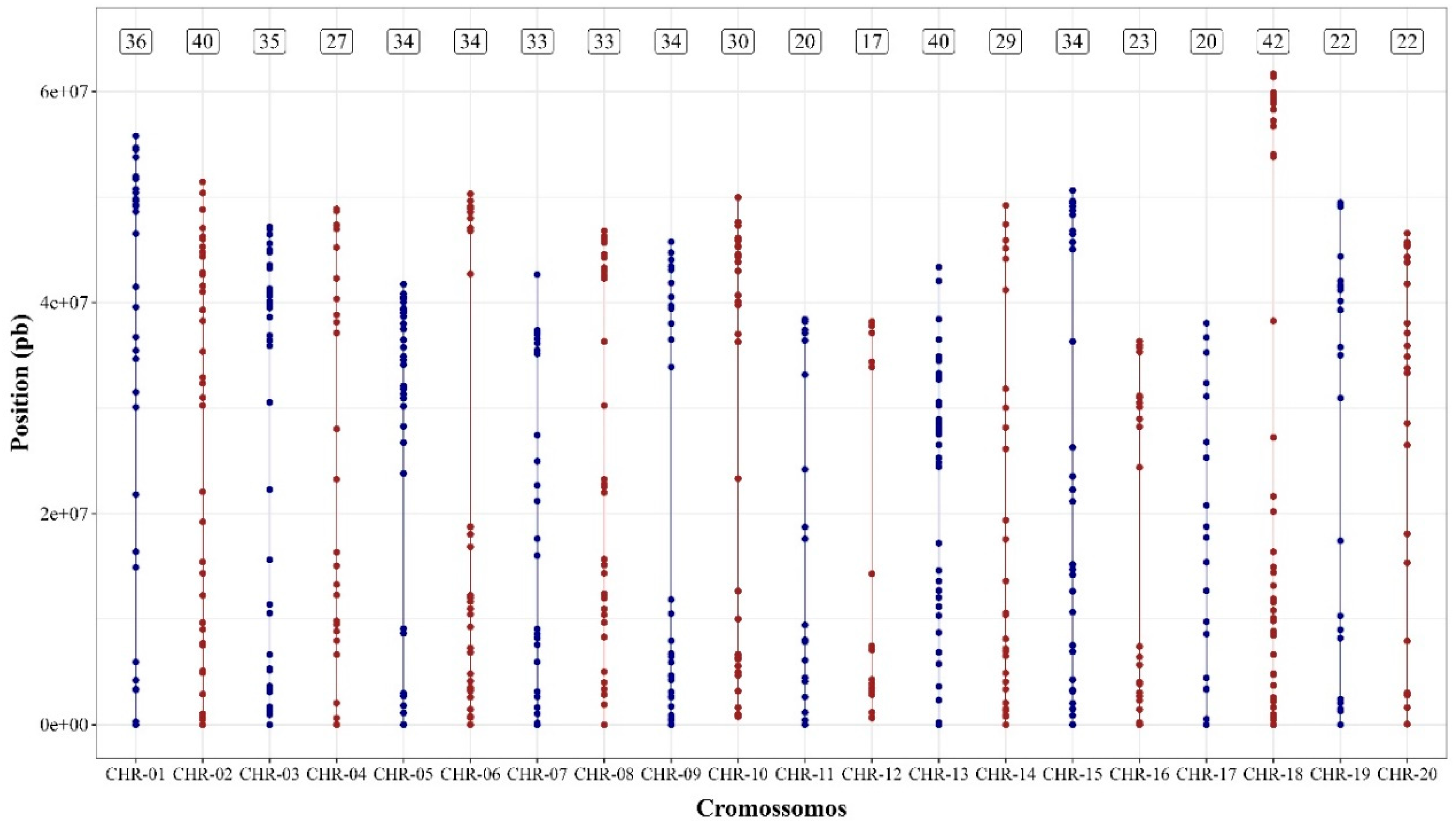
Figure 2.
Hierarchical Cluster Analysis Dendrogram of 267 Soybean Genotypes Based on Provesti’s Absolute Genetic Distance, derived from the analysis of 605 SNP markers, with the Mojena test applied to determine the optimal number of clusters.
Figure 2.
Hierarchical Cluster Analysis Dendrogram of 267 Soybean Genotypes Based on Provesti’s Absolute Genetic Distance, derived from the analysis of 605 SNP markers, with the Mojena test applied to determine the optimal number of clusters.
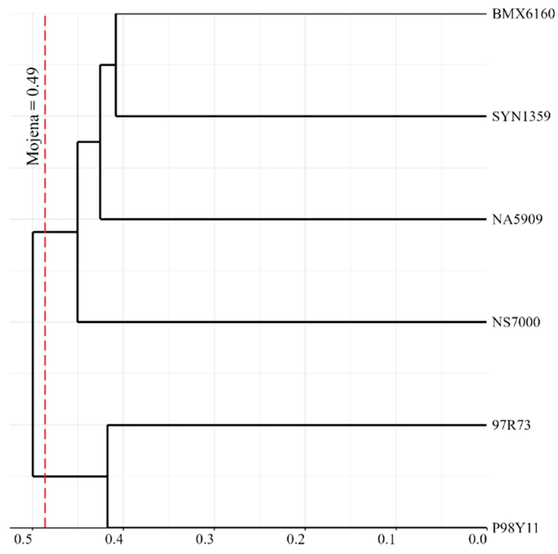
Figure 3.
Principal Component Analysis (PCA) Scatter Plot of Pairwise Genetic Distances Among 267 Progenies Using 605 SNP Markers.
Figure 3.
Principal Component Analysis (PCA) Scatter Plot of Pairwise Genetic Distances Among 267 Progenies Using 605 SNP Markers.
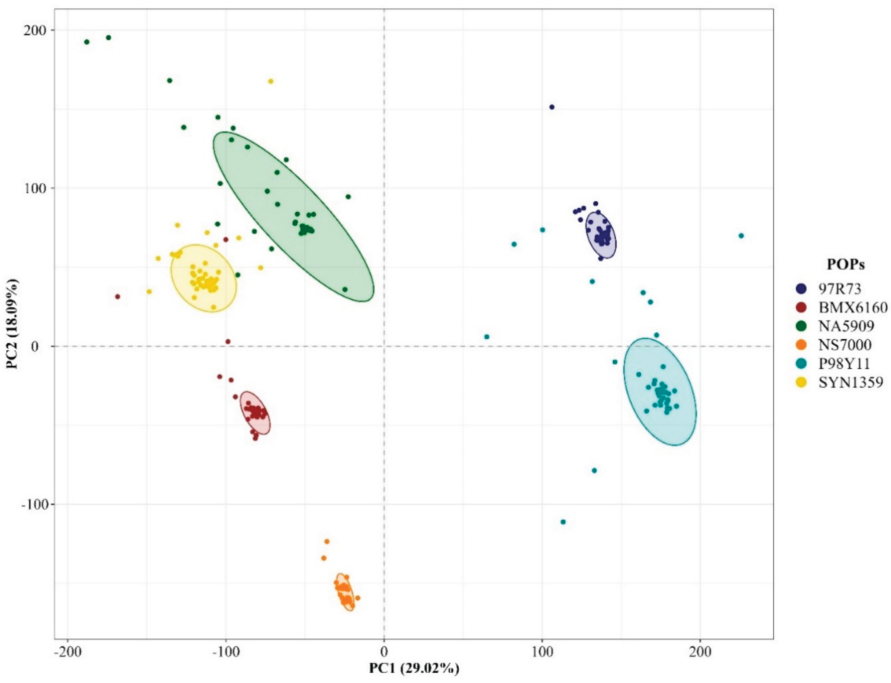

Table 1.
- Results for the multi-environment analysis for Days to Flowering (DF), Full Maturity (FM), Grain Yield (YIELD) and Plant Height (PH).
Table 1.
- Results for the multi-environment analysis for Days to Flowering (DF), Full Maturity (FM), Grain Yield (YIELD) and Plant Height (PH).
| SV | Effect | YIELD | PH | FM | DF |
|---|---|---|---|---|---|
| F | ns | ns | ** | ** | |
| R | ** | ** | ** | ns | |
| R | ** | ** | ** | ** | |
| R | ** | ** | ** | ** | |
| R | ** | ns | ** | ** | |
| R | ns | ** | ** | ** | |
| R | ns | ** | ** | ** | |
| R | ** | ** | ** | ** | |
| R | ** | ** | ** | ** | |
| R | ** | ** | ** | ** | |
| R | ns | ** | ** | ** | |
| R | ns | ns | ** | ** | |
| R | ** | ns | ** | ** | |
| - | 4655.08 | 76.44 | 115.13 | 45.19 | |
| - | 0.17 | 0.86 | 0.12 | 0.48 | |
| - | 0.18 | 0.96 | 0.86 | 0.96 | |
| - | 0.30 | 0.99 | 0.88 | 0.98 | |
| - | 0.41 | 0.93 | 0.35 | 0.69 | |
| - | 0.39 | 0.98 | 0.93 | 0.98 | |
| - | 0.55 | 0.99 | 0.94 | 0.99 | |
| (%) | - | 3.49 | 3.42 | 0.36 | 0.92 |
| (%) | - | 3.58 | 18.43 | 2.53 | 6.67 |
| (%) | - | 16.61 | 8.67 | 2.11 | 3.74 |
SV: Source of variation; mean square of checks, progenies variance, population variance, Variance among , , residual variance, DF and FM (days); PH (cm); YIELD (Kg ha-1); Wald test for fixed effects (F) and LRT (Likelihood Ratio Test) for random effects (R); "ns" indicates 'not significant', whereas asterisks (*) indicate levels of significance, with one asterisk for p < 0.05 and two asterisks for p < 0.01. : Heritability among populations; : heritability within populations modified; h²total: total heritability = heritability among + within populations modified;: accuracy on the progeny-mean basis; : accuracy on the population; : accuracy total; : population coefficient of variation in percentage; : coefficient of variation of progeny or progeny within population, in percentage terms; : experimental coefficient of variation in percentage terms.
Table 2.
Heterozygosity Metrics for Genetic Diversity Assessment within Populations using 605 SNP Markers. It includes information on Expected Heterozygosity (He), and Observed Heterozygosity (Ho).
Table 2.
Heterozygosity Metrics for Genetic Diversity Assessment within Populations using 605 SNP Markers. It includes information on Expected Heterozygosity (He), and Observed Heterozygosity (Ho).
| Population | He | Ho |
|---|---|---|
| SYN1359 | 0.0929 | 0.0700 |
| P98Y11 | 0.1245 | 0.1125 |
| BMX6160 | 0.0483 | 0.0360 |
| 97R73 | 0.0702 | 0.0477 |
| NS7000 | 0.0478 | 0.0321 |
| NA5909 | 0.0952 | 0.0897 |
Disclaimer/Publisher’s Note: The statements, opinions and data contained in all publications are solely those of the individual author(s) and contributor(s) and not of MDPI and/or the editor(s). MDPI and/or the editor(s) disclaim responsibility for any injury to people or property resulting from any ideas, methods, instructions or products referred to in the content. |
© 2025 by the authors. Licensee MDPI, Basel, Switzerland. This article is an open access article distributed under the terms and conditions of the Creative Commons Attribution (CC BY) license (http://creativecommons.org/licenses/by/4.0/).
Copyright: This open access article is published under a Creative Commons CC BY 4.0 license, which permit the free download, distribution, and reuse, provided that the author and preprint are cited in any reuse.


