Submitted:
10 September 2025
Posted:
11 September 2025
You are already at the latest version
Abstract
This paper presents a novel hybrid numerical scheme that combines the Finite Element Method (FEM) and Pseudospectral Methods to simulate he nonlinear transport of pollutants in water environments. The mathematical model is based on a convection-diffusion-reaction equation coupled with a stationary incompressible Navier-Stokes velocity eld. By leveraging the geometric exibility of FEM and the high spatial resolution of spectral techniques, the proposed method offers improved accuracy and stability, even under limited regularity of the solution. Numerical simulations are conducted to evaluate the influence of key physical parameters such as the Reynolds number and reaction nonlinearity. The results highlight the robustness of the method and provide insights into pollutant dynamics in environmental flow scenarios.
Keywords:
pollutant transport
; nonlinear reaction-diffusion equations
; finite element method
; pseudospectral method
; environmental fluid dynamics
1. Introduction
Water pollution is one of the most critical environmental challenges of the 21st century, particularly in natural watercourses that serve as essential reservoirs for biodiversity, drinking water, agriculture, and industry. The propagation of pollutants in rivers, lakes, and estuaries involves complex physical, chemical, and biological processes governed by fluid flow, dispersion, and reaction mechanisms [2,6,14]. Understanding and predicting these transport phenomena is crucial for environmental risk assessment, water quality management, and the design of remediation strategies [16].
Over the past decades, mathematical modeling and numerical simulation have become indispensable tools in environmental hydrodynamics. They offer a cost-effective alternative to experimental monitoring, which is often limited by spatial coverage, temporal resolution, or financial constraints [3,8]. Various numerical approaches have been proposed for simulating pollutant transport, including finite difference methods [13], finite volume methods [10], and finite element methods (FEM) [4]. While FEM provides flexibility in handling complex geometries, spectral and pseudospectral methods are known for their superior accuracy in resolving smooth solutions [1,15].
Hybrid numerical schemes that combine the geometric adaptability of FEM with the precision of spectral methods have gained attention in recent years, especially for advection-diffusion-reaction equations [9,12]. These methods can yield high-order accuracy while maintaining stability under stiff nonlinearities or irregular domains. However, their application to environmental flow problems-particularly those involving coupled Navier-Stokes and reaction-diffusion systems-remains under explored.
In this work, we propose a hybrid numerical approach that couples the finite element method with a pseudospectral discretization scheme to simulate the nonlinear transport of pollutants in a two-dimensional watercourse. The pollutant concentration is governed by a convection-diffusion-reaction equation, while the flow velocity is computed from the steady-state incompressible Navier-Stokes equations. The nonlinear reaction term models degradation or transformation processes that may occur during pollutant dispersion.
Our main contributions are as follows:
- We formulate a coupled nonlinear system for pollutant transport in incompressible flows, incorporating both diffusion and nonlinear reaction dynamics.
- We develop a hybrid FEM-pseudospectral scheme that ensures stability and convergence even under limited solution regularity.
- We conduct a set of numerical experiments to illustrate the effects of physical parameters (e.g., Reynolds number, reaction nonlinearity) on pollutant distribution.
The remainder of the paper is organized as follows: Section 2 presents the mathematical model and governing equations. Section 3 details the spatial discretization and hybrid numerical scheme. Section 4 describes the algorithmic implementation and simulations. Section 5 analyzes the numerical results. Finally, Section 6 concludes the paper with perspectives for future work.
We consider the transport and diffusion of a chemical pollutant in a two-dimensional, bounded aquatic domain , over a finite time interval . The pollutant concentration, denoted by , is governed by a convection?diffusion-reaction equation:
subject to homogeneous Neumann boundary conditions:
and an initial condition:
Here, is the steady, incompressible velocity field of the ambient fluid, and represents a nonlinear reaction term describing chemical transformation, biological decay, or pollutant degradation.
The nonlinear function is defined as:
where is a reaction rate constant and is a nonlinearity parameter.
This form is widely used to represent autocatalytic reactions, nonlinear degradation, or sorption-desorption phenomena in environmental models [11]. For example:
- When , the reaction is linear and corresponds to classical first-order kinetics.
- For , the nonlinearity introduces reaction acceleration with increasing concentration, modeling stronger pollutant self-interaction or saturation effects.
The use of also ensures continuous differentiability and generality across a wide class of power-law reaction models.
The velocity field is assumed to satisfy the steady incompressible Navier-Stokes equations:
with the nonlinear convective terms defined by:
Here, is the Reynolds number, a dimensionless parameter characterizing the ratio between inertial and viscous forces in the fluid:
where is the fluid density, U a characteristic velocity, L a characteristic length, and the dynamic viscosity. Low Reynolds numbers indicate diffusion-dominated flows, whereas higher values suggest convection-dominated regimes with stronger mixing effects.
The model is based on the following:
- The fluid is Newtonian, incompressible, and its velocity field is stationary (i.e., independent of time).
- The pollutant is passive: it does not affect the flow field (one-way coupling).
- There is no pollutant exchange across the domain boundaries (homogeneous Neumann conditions).
- The domain may be geometrically complex, but is fixed in time and two-dimensional.
These simplifications make the model tractable while retaining the essential features of pollutant transport dynamics in realistic environmental systems such as shallow rivers or estuarine channels.
2. Discretized Model and Numerical Scheme
To numerically solve the coupled system described in Section 2, we employ a hybrid spatial discretization strategy that combines the Finite Element Method (FEM) for geometric flexibility and a pseudospectral method for high accuracy on each element. The resulting semi-discrete system enables efficient simulation of nonlinear convection-diffusion-reaction phenomena.
The computational implementation is carried out in MATLAB®, which provides a flexible environment for assembling local-to-global transformations, handling sparse matrices, and integrating nonlinear dynamical systems.
2.1. Spatial Discretization Framework
Let be a conforming triangulation of the domain , consisting of triangular elements . Each physical triangle is associated with an affine mapping from the reference triangle
On each element, we define a local spectral basis using Dubiner polynomials [5], which are orthogonal and well-suited for spectral element methods on triangles.
Given N a local approximation parameter, representing the degree of the interpolation polynomial on each triangle, the global basis functions where and are constructed by mapping the local basis functions from to and extending them by zero outside the element:
The spectral Dubiner basis on the reference triangle is defined by:
where is the Jacobi polynomial of degree n and order .
A schematic representation of the local-to-global mapping process and the assembly of the global matrices is shown in Figure 1.
2.2. Steady-State Velocity Field Computation via Spectral-Galerkin Method
To compute the steady-state velocity field , we discretize the stationary incompressible Navier-Stokes equations using a Galerkin approach. For each triangular element , we formulate the weak form of the momentum equations (5) and (6), and approximate them by integrating against the local basis functions . This yields the following variational expression:
By employing pseudo-spectral differentiation, we define local differentiation matrices and over the element , such that for any function f defined on , the derivatives at the collocation points are approximated as:
where , , and are vectors containing the values of f and its partial derivatives with respect to x and y at the collocation points of .
Additionally, we introduce a quadrature matrix , which is a diagonal matrix whose entries correspond to quadrature weights associated with the collocation points on the reference triangle . This enables the approximation of integrals over as:
where is the Jacobian matrix associated with the affine transformation from the reference triangle to the physical element .
By applying the pseudo-spectral differentiation formula (16) and the quadrature approximation (17) to the local weak formulation (15), we obtain the following discrete system for each velocity component:
where the local stiffness matrix is defined as:
and the nonlinear convective term is discretized as:
Here, the vectors and contain the discrete values of the velocity components and source terms at the collocation points of . The notation refers to a diagonal matrix whose entries are those of the vector .
By assembling the local equations (18) over all triangular elements in the mesh, we obtain an assembled system in local numbering:
- is the concatenated vector obtained by stacking all local velocity vectors from each triangle ;
- is a block-diagonal stiffness matrix whose diagonal blocks are the local stiffness matrices ;
- is a block-diagonal matrix with each diagonal block equal to the quadrature matrix ;
- and are the concatenated vectors of the local nonlinear convective terms and the source terms , respectively.
All local contributions are related to the global degrees of freedom via a global transformation matrix , such that:
where is the vector of global unknowns for the i-th velocity component. Substituting the above transformation into the assembled local system (21), we obtain the global nonlinear system:
This system represents a large-scale nonlinear problem, where the unknown global velocity vectors and must also satisfy the discrete incompressibility condition (8) which is discretized using the same spectral differentiation framework. This results in the following global discrete constraint:
where and are block-diagonal matrices that assemble all local spectral differentiation matrices and , respectively.
2.3. Pollutant Concentration Update
Once the steady-state velocity field is computed, the pollutant transport equation is discretized in space using the same local spectral basis and quadrature framework as for the velocity field.
By multiplying the governing equation (1) by the basis function and integrating over a triangle , we obtain the weak formulation:
Proceeding as in the velocity formulation, the advective term is approximated using spectral differentiation and quadrature:
where is the vector of pollutant concentration values at the collocation points of .
The resulting semi-discrete approximation of (25) reads:
where we define:
and where denotes the evaluation of the nonlinear reaction term at the collocation points of .
Simplifying (27) and isolating the time derivative yields the local system of ODEs:
Aggregating these local systems for all , and using the same block matrix notation introduced earlier, we obtain the global system in local numbering:
where:
- is a block-diagonal matrix whose k-th diagonal block is ;
- is a block-diagonal matrix with blocks .
Finally, transforming this system into global numbering using the global-to-local mapping matrix and the local-to-global projection matrix , we arrive at the global semi-discrete formulation:
The semi-discrete problem in pollutant concentration thus consists of computing the global time-dependent solution over the time interval subject to the initial condition:
where is the vector of initial concentration values evaluated at the global collocation points.
2.4. Convergence, Stability, and Algorithmic Implementation
2.4.1. Convergence of the Discretized Velocity Field Problem
The discretization of the stationary incompressible Navier-Stokes equations using a spectral-Galerkin approach on triangular elements results in a nonlinear saddle-point problem, constrained by the discrete incompressibility condition. The convergence of the velocity field approximation hinges on two main aspects: the spectral approximation properties of the Dubiner basis functions and the regularity of the exact solution. Assuming that the exact velocity field lies in a Sobolev space for , the spectral element discretization achieves exponential convergence in space with respect to the polynomial degree N on each triangle, provided the mesh is quasi-uniform and the geometry is smooth or polygonal [7,9].
More precisely, let denote the discrete spectral solution obtained from system (23) and the exact solution of the continuous weak problem. we can state the following result:
Theorem 1.
Let be a polygonal domain, and suppose the exact velocity field for some . Let denote the discrete velocity field obtained from the spectral-Galerkin system (23) using polynomial degree N on each triangle. Then, there exists a constant , independent of N, such that:
If is analytic on Ω, then the convergence is spectral, i.e., exponentially fast:
for some .
Proof.
The proof follows classical approximation theory for spectral element methods [7,9]. On each triangle , the spectral basis formed by Dubiner polynomials yields an approximation error of order in and in , due to inverse inequalities. The assembly of the global error estimate then follows from a Céa-type lemma applied to the discrete weak formulation of (15), using the inf-sup stability of the discrete spaces under suitable projection or stabilization. The exponential convergence in the analytic case comes from the classical result on orthogonal polynomial approximation of analytic functions on triangles. □
2.4.2. Convergence, Stability, and Algorithmic Implementation of the Semi Discretized Pollutant Problem
The semi-discrete formulation derived above leads to a system of nonlinear ordinary differential equations (ODEs) for the pollutant concentration . To guarantee the well-posedness and convergence of the numerical solution, we must ensure stability and boundedness of the solution over time.
2.4.2.1. Energy Boundedness Condition
We assume that the nonlinear reaction term satisfies the following dissipative condition:
Under this assumption, one can derive an energy estimate by multiplying equation (31) by and applying symmetry properties of the matrices involved. This yields:
where is the discrete weighted norm. By applying Grönwall’s inequality, this implies boundedness of the solution for all provided that remains small compared to the diffusion and advection damping rates.
2.4.2.2. Time Discretization and Solver Strategy
Rather than designing an ad-hoc time integrator, we advance the semi-discrete system obtained after spatial discretization by calling MATLAB’s built-in adaptive ODE solver. Denote by
with initial condition ; the steady velocity field is precomputed once and kept fixed during the concentration update. We then solve the IVP
by invoking MATLAB’s adaptive solver ode15s. This black-box approach automatically controls the time step to meet user-specified tolerances, and it avoids any custom IMEX design.
2.4.2.3. MATLAB Solver-Based Workflow
The implementation proceeds as follows:
- Precompute constant operators: assemble sparse matrices and (kept fixed if the velocity is steady), and prepare a function for the nonlinear reaction vector evaluated at .
- Define the RHS callback for the ODE solver:
- Call the solver with the desired tolerances:
- Post-process at requested output times, and map to local or physical fields via when needed.
3. Numerical Experiments
This section presents numerical experiments to validate and illustrate the performance of the proposed spectral-Galerkin framework for solving the coupled Navier–Stokes and pollutant transport equations. The simulations are implemented in MATLAB R2024a, leveraging sparse matrix operations and customized local-to-global assembly routines. Two main components are addressed: the steady-state velocity field computation and the transient pollutant concentration evolution.
The simulations are implemented in a modular MATLAB framework. Key features include:
- Local-to-global transformation via sparse matrix .
- Assembly of spectral differentiation matrices , using Jacobi or Dubiner basis.
- Block-diagonal structures for stiffness and convection matrices for efficient matrix- vector operations.
- Divergence enforcement via projection on .
- Time integration for concentration handled with vectorized Runge–Kutta schemes.
3.1. Numerical Resolution Strategy for the Discrete Velocity Field
The discrete system governing the steady-state velocity field, given in (23) together with the incompressibility constraint (24), results in a large-scale nonlinear algebraic problem. Direct solvers quickly become computationally prohibitive as the number of elements and polynomial degree increase, due to the size and sparsity pattern of the global matrices. To overcome this limitation, we adopt an efficient iterative scheme based on gradient methods, implemented in MATLAB.
3.1.0.4. Linearization
At each nonlinear iteration, the convective terms are linearized around the current velocity approximation . This yields a Jacobian-based correction system of the form:
where is the Jacobian matrix of the nonlinear operator, the correction, and the nonlinear residual.
3.1.0.5. Gradient-Based Solver
The correction system is solved iteratively using a preconditioned conjugate gradient (PCG) method. This choice exploits the symmetry and sparsity of the discretized operators, significantly reducing memory requirements and computation time. In MATLAB, this is implemented via the built-in operator solve (equivalent to mldivide) applied to the sparse Jacobian system, with the gradient iterations handled internally. For large problems, additional preconditioners such as incomplete LU (ILU) or Jacobi can be specified.
3.1.0.6. Algorithm
The overall resolution strategy is summarized as follows:
- Initialize with an admissible velocity field satisfying the discrete incompressibility constraint (24).
- At iteration m, assemble the nonlinear residual and the Jacobian .
- Solve the linear correction systemusing MATLAB’s solve with a gradient-based iterative scheme.
- Update the velocity field: .
- Enforce the incompressibility condition (24) by projecting the updated velocity field onto the divergence-free subspace.
- Repeat until convergence: , with tolerance .
3.1.0.7. Implementation in MATLAB
The following schematic illustrates the key commands:
J = assembleJacobian(v);
R = assembleResidual(v);
delta_v = J \ (-R); % equivalent to solve(J, -R) in MATLAB
v_new = v + delta_v;
Thanks to MATLAB’s efficient sparse linear algebra routines, the above approach enables the rapid computation of the velocity field even on fine meshes and for higher-order polynomial approximations.
This gradient-based resolution strategy ensures both computational efficiency and numerical stability, and is integrated into the global simulation framework presented in Section 3.2.
3.2. Manufactured Velocity Field for Convergence Verification
To validate the convergence properties of the method, we consider a manufactured solution defined on :
which is divergence-free and satisfies homogeneous Neumann conditions on the boundary. The corresponding source term is computed by substituting into the steady Navier–Stokes equations.
The numerical velocity field is computed on pseudo spectal collocation points on triangular meshes using polynomial degree . The errors between and the vector values of the exact solution at pseudo spectral collocation points are evaluated. Table 1 reports the exponential decay of the errors, confirming spectral convergence.
A convergence plot (Figure 2) confirms the exponential accuracy of the scheme with respect to the polynomial order N.
3.3. Numerical Simulation of the Coupled Velocity–Concentration System
To assess the performance of the proposed spectral–Galerkin discretization in a realistic setting, we simulate the coupled velocity and pollutant transport problem described in Section 2. The computational domain corresponds to a river channel containing a central islet, which introduces geometric complexity and induces heterogeneous flow patterns. The domain is discretized into 119 triangular spectral elements using a mesh generator (see Figure 3). Unless otherwise specified, we fixe , while the influence of the nonlinear reaction parameter and the advection strength parameter are systematically investigated. The polynomial order of the pseudospectral approximation is set to throughout all computations. The Reynolds number is prescribed as , and the forcing term is identical to that employed in the steady-state velocity computation described earlier.
Simulation Setup
The simulation proceeds in two stages. First, the steady-state velocity field is computed by solving the nonlinear system (23) subject to the incompressibility constraint (24). The resulting velocity profiles are then used as input data for the transient pollutant transport problem governed by the semi-discrete system (31). Time integration of the concentration field is performed with a second-order explicit Runge–Kutta method, which provides a good balance between accuracy and computational efficiency. Homogeneous Neumann boundary conditions are prescribed for the concentration, enforcing a no-flux condition at the riverbanks and islet boundary. The pollutant is initially localized in the vicinity of a prescribed interior point of , mimicking the instantaneous release of a contaminant source.
Test Scenarios
Several test cases are conducted to quantify the effect of nonlinear reaction dynamics. In particular, the role of the parameter in shaping the pollutant distribution is examined by varying its value over a wide range, while controls the intensity of pollutant diffusion. Unless otherwise noted, a reference configuration with and is considered.
Results: Velocity Field
Figure 4 illustrates the steady-state velocity field for . The computed streamlines highlight the strong influence of the islet on the overall flow structure, with the formation of recirculation zones and regions of locally accelerated flow. For higher Reynolds numbers (e.g., ), the velocity gradients become sharper, leading to enhanced advective transport in the downstream region.
Results: Pollutant Transport
The pollutant transport simulations reveal the interplay between advection, diffusion, and nonlinear reaction. Figure 5 shows the temporal evolution of the concentration field for . The pollutant plume initially spreads due to local diffusion, while advection progressively transports the contaminant along streamlines. Over time, nonlinear reactions amplify concentration gradients, leading to heterogeneous accumulation patterns within the domain.
The influence of the nonlinear reaction parameter is further analyzed in Figure 6 and Figure 7, which display the pollutant concentration at for . Increasing results in pronounced pollutant accumulation near the riverbanks and around the islet boundary, demonstrating the critical role of reaction terms in shaping long-term pollutant patterns.
Discussion
The numerical experiments confirm the robustness and accuracy of the proposed spectral–Galerkin discretization for coupled velocity–concentration problems. The method remains stable for complex geometries and polynomial degrees up to . The results highlight the following major physical effect:
- Increasing enhances pollutant accumulation near boundaries and reactive hotspots, reflecting the dominant role of nonlinear reaction kinetics.
Overall, the spectral–Galerkin approach proves effective for capturing intricate nonlinear interactions between fluid flow and pollutant dynamics, making it a promising tool for large-scale environmental flow simulations.
4. Conclusions
In this work, we developed a hybrid numerical framework that combines the Finite Element Method (FEM) and Pseudospectral techniques to simulate the nonlinear diffusion and advection of pollutants in a two-dimensional aquatic environment. The proposed method addresses the challenges posed by complex geometries and nonlinear reaction terms by leveraging the geometric flexibility of FEM and the high resolution of spectral discretizations.
We formulated a coupled system involving the stationary incompressible Navier-Stokes equations for fluid velocity and a nonlinear convection-diffusion-reaction equation for pollutant concentration. A detailed numerical scheme was presented, along with two modular algorithms for solving the velocity and concentration fields efficiently. Our simulations demonstrated the robustness and accuracy of the method under varying Reynolds numbers and nonlinear reaction parameters.
Key observations include the method’s numerical stability across a range of discretization parameters and the pronounced sensitivity of pollutant accumulation patterns to the nonlinearity parameter . These insights underscore the importance of accurately modeling reaction kinetics in water quality simulations.
Future work may extend this framework to three-dimensional domains, incorporate time-dependent velocity fields, or account for multi-species transport and reactive boundary conditions. Furthermore, integrating real-world data or coupling with watershed models could enhance the method’s applicability in environmental decision-making and pollution mitigation strategies.
References
- Canuto, C. , Hussaini M. Y., Quarteroni A., Zang T. A., Spectral Methods: Evolution to Complex Geometries and Applications to Fluid Dynamics, Springer, 2007.
- Chapra S., C. , Surface Water-Quality Modeling, McGraw-Hill, 1997.
- Cunge J., A. , Holly, F. M., Verwey, A., Practical Aspects of Computational River Hydraulics, Pitman Publishing, 1980.
- Donea, J. , and Huerta, A., Finite Element Methods for Flow Problems, Wiley, 2003.
- Dubiner, M. , Spectral methods on triangles and other domains, Journal of Scientific Computing, 6(4), 345-390, 1991. [CrossRef]
- Fischer H., B. , List, E. J., Koh, R. C. Y., Imberger, J., Brooks, N. H., Mixing in Inland and Coastal Waters, Academic Press, 1979.
- Hesthaven J., S. , Gottlieb S. and Gottlieb D., Spectral Methods for Time-Dependent Problems, Cambridge University Press, 2007.
- Jobson H., E. , Predicting travel time and dispersion in rivers and streams, Journal of Hydraulic Engineering, Volume 123, Issue 11, 1997. [CrossRef]
- Karniadakis G., E. , Sherwin S. J., Spectral/hp Element Methods for Computational Fluid Dynamics, Oxford University Press, 2005.
- LeVeque R., J. , Finite Volume Methods for Hyperbolic Problems, Cambridge University Press, 2002.
- Murray J., D. , Mathematical Biology I: An Introduction, Springer, 2002.
- Sherwin S., J. , Karniadakis G. E., A new triangular and tetrahedral basis for high-order finite element methods, International Journal for Numerical Methods in Engineering, 38(22), pp.3775-3802, 1995.
- Smith G., D. , Numerical Solution of Partial Differential Equations: Finite Difference Methods, Oxford University Press, 1985. [CrossRef]
- Thomann R., V. , and Mueller, J. A., Principles of Surface Water Quality Modeling and Control, Harper Collins, 1997.
- Trefethen L., N. , Spectral Methods in MATLAB, SIAM, 2000.
- Zoppou, C. , Review of urban storm water models, Environmental Modelling &; Software, 16(3): 195 - 231, 2001. [Google Scholar]
Figure 1.
Illustration of the transformation from local reference triangle to global triangulated domain using affine mappings , and the local-to-global matrix assembly.
Figure 1.
Illustration of the transformation from local reference triangle to global triangulated domain using affine mappings , and the local-to-global matrix assembly.
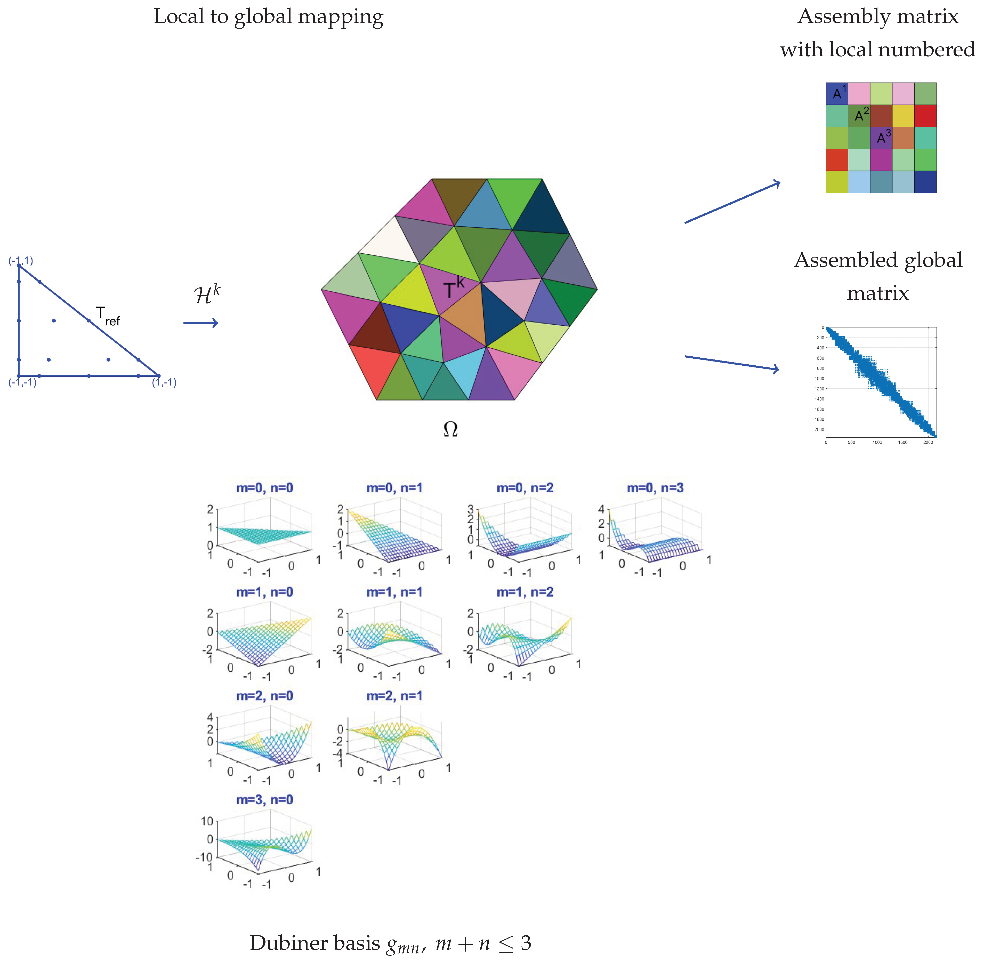
Figure 2.
The exact velocity field (left) and the onvergence of the velocity field error in -norm as a function of N(right).
Figure 2.
The exact velocity field (left) and the onvergence of the velocity field error in -norm as a function of N(right).
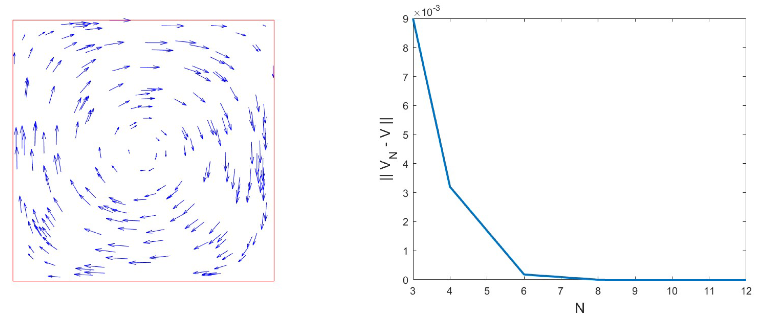
Figure 3.
Computational domain representing a river channel with an embedded islet, discretized into 119 triangular spectral elements.
Figure 3.
Computational domain representing a river channel with an embedded islet, discretized into 119 triangular spectral elements.
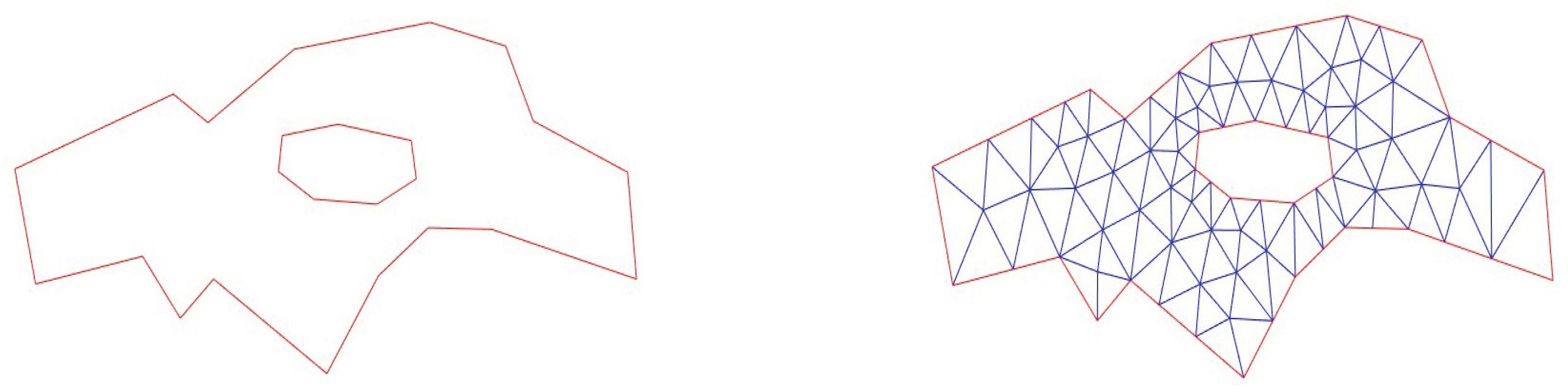
Figure 4.
Computed steady-state velocity field for . The islet generates recirculating vortices and strong velocity gradients near its boundary.
Figure 4.
Computed steady-state velocity field for . The islet generates recirculating vortices and strong velocity gradients near its boundary.
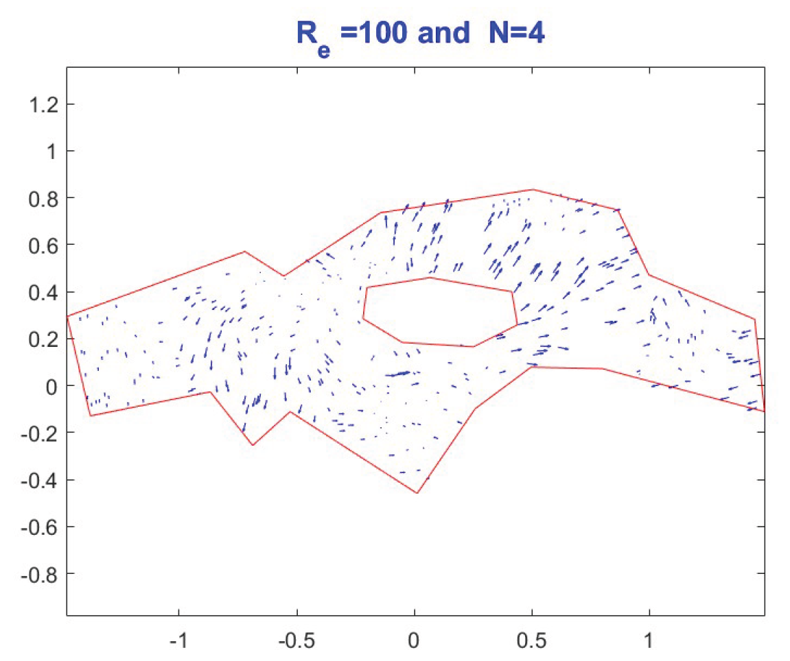
Figure 5.
Time evolution of pollutant concentration for and . The plume exhibits combined effects of advection and nonlinear reaction.
Figure 5.
Time evolution of pollutant concentration for and . The plume exhibits combined effects of advection and nonlinear reaction.
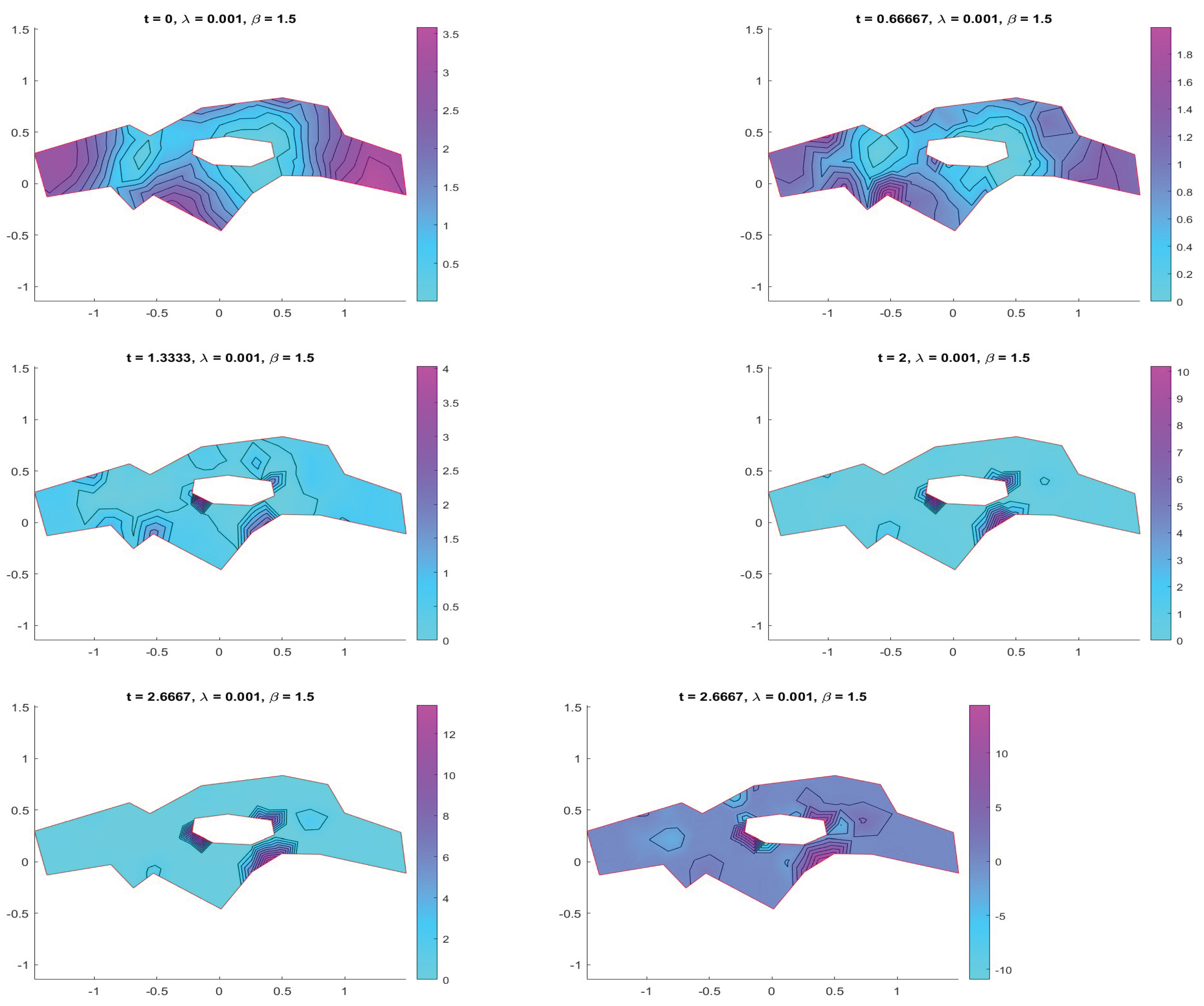
Figure 6.
Pollutant distribution at for (left) and (right).
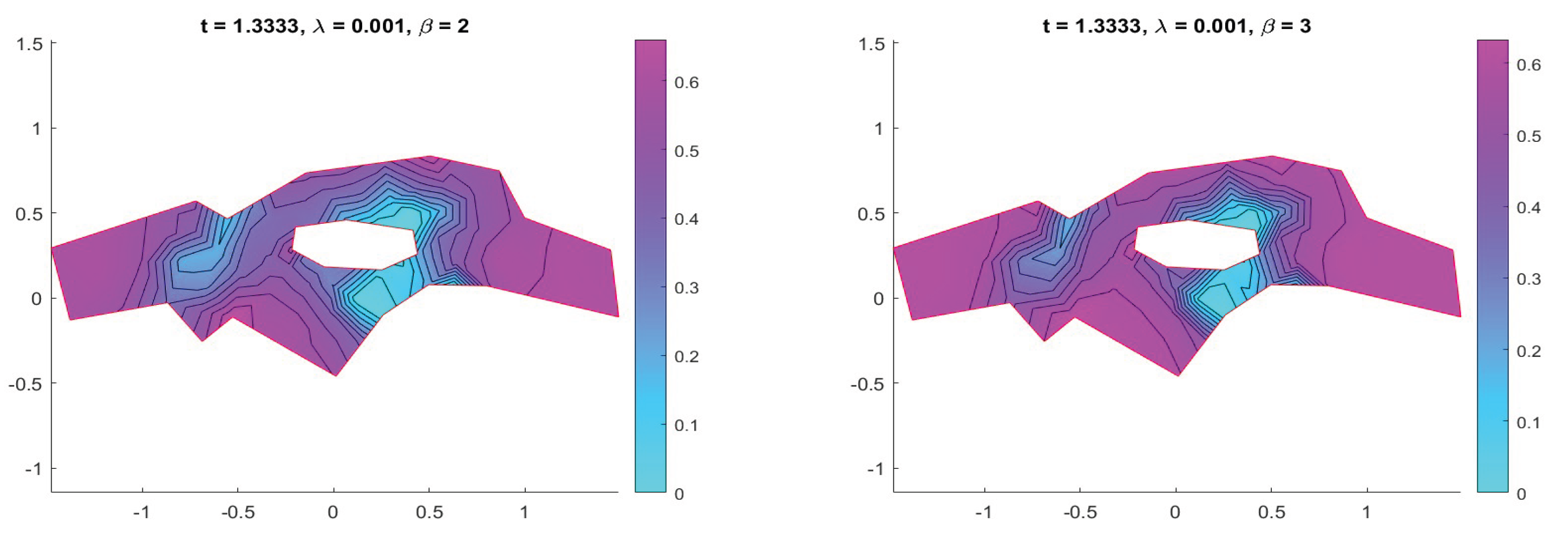
Figure 7.
Pollutant distribution at for (left) and (right).
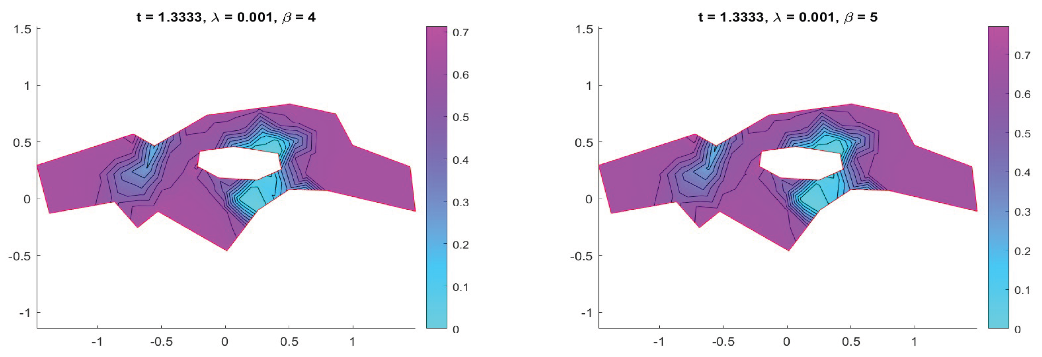

Table 1.
errors for velocity field vs polynomial degree N.
| N | 4 | 6 | 8 | 10 |
|---|---|---|---|---|
Disclaimer/Publisher’s Note: The statements, opinions and data contained in all publications are solely those of the individual author(s) and contributor(s) and not of MDPI and/or the editor(s). MDPI and/or the editor(s) disclaim responsibility for any injury to people or property resulting from any ideas, methods, instructions or products referred to in the content. |
© 2025 by the authors. Licensee MDPI, Basel, Switzerland. This article is an open access article distributed under the terms and conditions of the Creative Commons Attribution (CC BY) license (http://creativecommons.org/licenses/by/4.0/).
Copyright: This open access article is published under a Creative Commons CC BY 4.0 license, which permit the free download, distribution, and reuse, provided that the author and preprint are cited in any reuse.


