
Submitted:
08 September 2025
Posted:
11 September 2025
You are already at the latest version
Abstract
In this study, we introduce a Transformer-based forecasting tool termed EXPERT (EXchange rate Prediction using Encoder Representation from the Transformers) and apply it to the domain of exchange rate forecasting. To achieve this, we first developed and trained the Transformer-based forecasting model; we then evaluated its performance on a diverse set of 9 currency pairs with various characteristics. Finally, we benchmarked its effectiveness against six established and respected forecasting models: Linear Regression, Random Forests, Stochastic Gradient Descent, XGBoost, Bagging Regression, and Long Short-Term Memory. Our dataset covers the period from 1999 to 2022. The models were evaluated for their ability to predict the next day's closing price using three performance metrics. In addition, the EXPERT system was evaluated for extending forecast horizons and as the core of a trading strategy. The universal robustness of the proposed model was tested using the Multiple Comparisons with the Best (MCB) on five samples of our dataset.
Keywords:
Exchange rates
; Time series forecasting
; Deep Learning
; Transformers
1. Introduction
The Foreign Exchange (FOREX) market, a global behemoth in financial exchange, facilitates the continuous, 24/5, trade of currencies across diverse participants and time zones, thereby acting as a vital conduit for international trade, investment, and risky speculation.
The FOREX ecosystem involves a multitude of actors, including multinational corporations engaged in cross-border trade, governments making strategic interventions, central banks shaping monetary policies, financial institutions providing liquidity and market-making services, and individual traders venturing into the online arena. Despite its complexity and inherent volatility, the FOREX market attracts traders and investors due to features like short trading and leverage. FOREX allows short selling, which is the act of selling a currency that the agent does not currently own, with the commitment to buy it in the near future.
Exchange rates, reflecting the relative value of one currency compared to another, can be classified based on their regime (fixed or floating) and type (nominal or real). Fixed exchange rates, dictated by governments or central banks, remain constant, while floating rates are determined by supply and demand. Nominal exchange rates represent the current market value of a currency pair, while real exchange rates account for inflation. The flexibility of floating rates allows currencies to adapt to changing economic conditions, facilitating trade and investment flows, promoting price stability, and maintaining external balance. The exchange rates of major reserve currencies such as the US dollar (USD), the Euro (EUR), the Japanese Yen (JPY), the British Pound Sterling (GBP) hold significant importance in the global economic landscape due to their crucial role in international trade and financial transactions.
Accurate exchange rate forecasts are crucial for various market participants, including traders, investors, businesses, and policymakers. These predictions inform decisions about currency trades, asset allocation, and risk management, ultimately impacting portfolio performance. Businesses and policymakers rely on these models to plan and execute international transactions, manage foreign currency exposure, and mitigate risks associated with currency fluctuations. Additionally, they play a role in formulating effective monetary and fiscal policies aimed at achieving macroeconomic stability, managing inflation, and fostering sustainable economic growth.
Traditionally, exchange rate forecasting relied on fundamental and technical analysis. Fundamental analysis involves studying economic indicators like interest rates, inflation, GDP growth, trade balances, and even geopolitical developments to understand the underlying factors driving currency movements. Technical analysis, on the other hand, focuses on historical price data, chart patterns, and technical indicators to identify trends and predict future price movements. It is important to note that expert opinions, intuition, and qualitative judgments are sometimes used. However, their success rate can vary dramatically.
In recent years, a paradigm shift has occurred, with advanced computational techniques like machine learning (ML) and artificial intelligence (AI) making inroads into exchange rate forecasting. These approaches leverage big data analytics, deep learning, and neural networks to process vast amounts of financial data, identify complex patterns, and generate precise predictions. Deep learning models have proven particularly effective, demonstrating superior predictive capabilities compared to traditional methods [1]. Their ability to capture non-linear relationships, temporal dependencies, and high-dimensional features inherent in financial time series data sets them apart. Classic architectures like Convolutive Neural Networks (CNN) and Recurrent Neural Networks (RNN) have limitations. For instance, CNN pooling layers disregard crucial part-whole correlations and lose valuable data, while RNNs are prone to gradient vanishing or exploding issues during backpropagation.
Addressing these challenges, Vaswani et al., (2017) [29] introduced the Transformer, a novel deep learning model. This model, originally excelling in natural language processing (NLP) tasks, replaces traditional CNN and RNN frameworks with an attention mechanism. Unlike the sequential structure of RNN and LSTM, the Transformer’s self-attention mechanism can be trained in parallel and requires less complexity to gather global information.
While Transformer architectures have revolutionized NLP tasks such as machine translation and language modeling, financial institutions are exploring its ability to tackle the complexities of financial time series forecasting. This integration holds immense potential due to the inherent challenges associated with predicting financial market behavior. Additionally, advancements in computing technology and data availability have facilitated the widespread adoption of Transformer-based models by academic researchers seeking an edge in currency trading and investment strategies.
Advancements in technology alone are not a panacea, especially when considering the recent complexities in the FOREX market, such as the fluctuations caused by the COVID-19 pandemic and the Russia-Ukraine conflict. These events posed significant challenges for traders in predicting currency pair movements, as economic factors, sentiment, and geopolitical developments all played a significant role in shaping exchange.
Inspired by the success of Transformers in modeling sequential data in NLP, the same concept is employed in this study to forecast the evolution of exchange rates in the FOREX market. While recent studies have explored their use for trading purposes [2,3,4,5], we focus on the use of Transformers for next-day closing price prediction, which to the best of our knowledge is the first effort of its kind in the FOREX.
In their analysis, Fisher et al., [4] examine Transformer models with time embeddings for FX-Spot forecasting, comparing results with traditional models like LSTM for major currency pairs (EUR/USD, USD/JPY, GBP/USD) from November 2020 to January 2022. Their method includes both univariate and multivariate models, utilizing historical prices along with technical and fundamental data. Findings reveal that Transformers significantly outperform LSTM. Transformers demonstrated strength in noisy, high-frequency environments, proving effective for complex financial series.
Gradzki & Wojcik [3] focus on high-frequency Forex trading with Transformers, comparing them to ResNet-LSTM across six currency pairs and five time intervals (60 to 720 minutes). This study employs a Transformer architecture for forecasting, enhanced by technical analysis for improved accuracy. The findings indicate that Transformers slightly outperform ResNet-LSTM, especially in longer intervals (480, 720 minutes). However, transaction costs significantly impact performance in shorter intervals (e.g., 60 minutes), underscoring the necessity for realistic backtesting.
Exploring a Transformer Encoder model for minute-level Forex trading, [5] specifically focus on EURUSD and GBPUSD. The model integrates Exponential Moving Averages (EMA) with varying smoothing factors to better capture price trends. Trained on data from July 2023, it achieves a cross-entropy loss below 0.2, indicating strong predictive accuracy. However, profitability is limited by high-frequency trading costs, as spreads can negate gains, demonstrating that real-world outcomes are significantly affected by transaction costs.
In a significant contribution, Kantoutsis et al., [2] presents the Momentum Transformer, an attention-based deep learning model that outperforms traditional momentum and mean reversion strategies, as well as LSTM-based models. By leveraging attention mechanisms, it captures long-term dependencies and adapts to market shifts, such as those seen during the SARS-CoV-2 crisis. Back-testing from 1995 to 2020 reveals superior performance, particularly in recent years and during significant market events. While the hybrid Temporal Fusion Transformer (TFT) performed best overall, pure attention models also demonstrated strong performance. The study suggests an ensemble approach for improved results across asset classes and highlights the model’s robustness in commodities trading.
In our approach we test the forecasting ability of our Transformer-based model, called EXPERT on 9 currency pairs: EUR/USD, AUD/CAD, EUR/AUD, EUR/CAD, GBP/AUD, NZD/USD, USD/JPY, USD/MXN, BRL/USD and evaluate it against six widely used forecasting models: the Stochastic Gradient Descent (SGD), the Bagging Regression (BGR), the Extreme Gradient Boosting (XGB), the Random Forests (RF), the Linear Regressor, and the Long Short-Term Memory (LSTM) model.
Each dataset for these 9 currency pairs has been individually used in every forecasting model, using the classic training - testing scheme. The training set is utilized to fine-tune the parameters of the model; the performance of the trained models is evaluated on the testing set. All models predict the closing price for the next day. The estimated value is then evaluated with the actual values.
The paper is organized as follows. Section 2 reviews related work, while Section 3 presents the collected dataset. Every aspect of the EXPERT model is analyzed in Section 4. The alternative forecasting models are briefly introduced in Section 5. Section 6 presents the evaluation metrics used. The forecasting performance of the EXPERT model against the competition is presented in Section 7. In the same section, we present the performance of the EXPERT model for larger forecasting horizons and evaluate its performance using the Multiple Comparisons with the Best method on five samples from our dataset. In Section 8, we evaluate the success of a Transformer-based automatic trading system against other similar systems, and in Section 9, we conclude the paper.
2. Related work
A systematic review of the existing literature was conducted to gain a comprehensive understanding of machine learning prediction models in exchange rates [6,7,8,10].
The improvements reported for neural networks in the paper by Islam et al., [10] focus on a hybrid GRU-LSTM model that outperforms standalone GRU and LSTM models, as well as a simple moving average (SMA) model, across several performance metrics, including the MSE, RMSE, MAE, and R2 score. Comparisons were made against these benchmarks to demonstrate the efficacy of the proposed model. The models were tested on historical foreign exchange data for four major currency pairs: EUR/USD, GBP/USD, USD/CAD, and USD/CHF, using a data set that spans from January 1, 2017, to June 30, 2020. The hybrid model was specifically applied to predict the closing prices of these currency pairs for both 10-minute and 30-minute timeframes, highlighting its superior predictive capabilities.
In their study on exchange rate prediction, Panda et al., [8] reveal that a hybrid GRU-LSTM model effectively predicts future closing prices in the FOREX market. Applied to major currency pairs (EUR/USD, GBP/USD, USD/CAD, USD/CHF), this model outperformed standalone GRU, LSTM, and simple moving average (SMA) models in terms of MSE, RMSE, and MAE for 10-minute intervals, and excelled with GBP/USD and USD/CAD in 30-minute intervals. It also achieved a higher score, indicating a lower prediction risk. Using a dataset of closing prices from January 1, 2017, to June 30, 2020, the model showed strong predictive capabilities, though it struggled during sudden price fluctuations. Future enhancements are planned, including applications to more currency pairs and shorter timeframes.
The key findings of the paper [7] emphasize the significant advantages of machine learning algorithms over traditional stochastic models in financial market forecasting. After surveying more than 150 relevant articles, the study demonstrates that machine learning algorithms generally outperform stochastic methods by effectively capturing nonlinear dynamics in financial time series across various asset classes and market geographies. Recurrent neural networks (RNNs) exhibit superior performance compared to feedforward neural networks and support vector machines, likely because of their ability to leverage temporal dependencies.
The paper of Seze et al., [6] reviews significant advancements in deep learning (DL) models for financial time series forecasting, showcasing their superiority over traditional machine learning approaches. Long Short-Term Memory (LSTM) networks are favored for their effectiveness in handling time-varying data and capturing temporal dependencies. More than half of the studies surveyed focus on recurrent neural networks (RNNs) for price trend predictions, while deep multilayer perceptrons (DMLPs) are often used for classification tasks. In addition, there is increasing interest in deep reinforcement learning (RL) for algorithmic trading, offering new opportunities to integrate behavioral finance insights.
Fletcher [9] demonstrates that machine learning techniques can theoretically be applied to make accurate currency predictions. Their findings indicate that it is possible to forecast the direction of movement (up, down, or within the bid-ask spread) of the EUR/USD pair between 5 and 200 seconds into the future, with accuracy rates ranging from 90% to 53%, respectively. Additionally, they have shown that it is feasible to predict price turning points for a basket of currencies in a way that can be profitably exploited.
Goncu [20] applied machine learning regression methods—Ridge, decision tree, support vector, and linear regression—to predict monthly average exchange rates, focusing on the USD/TRY (Turkish Lira). Key macroeconomic factors, such as domestic money supply, interest rates, and the prior month’s exchange rate, are used for prediction. Among the tested models, Ridge regression delivers the most accurate forecasts, with relative errors under 60 basis points. Out of sample back-testing over various time periods confirms Ridge’s superior performance, suggesting it effectively balances accuracy and overfitting. The model can also be used for scenario analysis, helping policymakers and investors assess the impact of interest rate changes on exchange rates.
Research by Qi et al., [18] introduces event-driven features to improve Forex trading predictions by identifying trend changes and retracement points for optimal trade entry. The authors tested deep learning models, including LSTM, BiLSTM, and GRU, against a baseline RNN, with GRU and BiLSTM outperforming the others across various currency pairs. The best model, GRU with 60 timesteps for EUR/GBP, achieved an RMSE of 1.50x and a MAPE of 0.12%, surpassing previous studies. These findings show that the proposed models, combined with event-driven features, can provide accurate, low-risk trading strategies.
The development of more advanced models has been proposed from Islam & Hosssain [19] where they introduced a network combining the GRU with the LSTM for improved FOREX rate prediction.
3. The Dataset
In this study, our objective is twofold: a) to create a Transformer-based model (EXPERT) for forecasting exchange rates and b) to test it against a set of well-known forecasting methodologies. To ascertain the overall most accurate forecasting model, we must test them on a rich and diverse dataset that includes exchange rates with different characteristics. Testing our models on multiple pairs helps to mitigate the risk of overfitting to the specific market characteristics present in a single currency pair, increasing the model’s reliability and applicability to real-world trading scenarios. The dataset was compiled using the Metatrader application and comprises two major, five minor, and three exotic exchange rates, spanning the period from January 1999 to March 2022 for the weekdays. Each entry in the dataset contains the Open, High, Low, and Close values.
The dataset was divided into training, validation, and testing sets. The first 86% of the data was used for training, with an internal validation split of 10%, meaning that 68.8% of the total dataset was used for training and 17.2% for validation. The remaining 14%, which is our testing subset, was used as a validation (out-of-sample) data to evaluate the models’ ability to generalize to new, unseen data. A sliding window approach was applied to create sequences for both the training and testing phases, allowing the model to capture temporal dependencies. This data-splitting strategy provided a robust evaluation of the model’s performance across both the training and out-of-sample data.
The currency pairs exchange rates were categorized as major, minor, or exotic based on the European Securities and Markets Authority (ESMA). In this context, the currency pairs in our datasets are classified as:
Major Currency Pairs:
- EUR/USD (Euro/US Dollar)
- USD/JPY (US Dollar/Japanese Yen)
Minor Currency Pairs (Cross Currency Pairs):
- 3.
- EUR/AUD (Euro/Australian Dollar)
- 4.
- EUR/CAD (Euro/Canadian Dollar)
- 5.
- AUD/CAD (Australian Dollar/Canadian Dollar)
- 6.
- GBP/AUD (British Pound/Australian Dollar)
- 7.
- NZD/USD (New Zealand Dollar/US Dollar)
Exotic Currency Pairs:
- 8.
- USD/MXN (US Dollar/Mexican Peso)
- 9.
- BRL/USD (Brazilian Real/US Dollar)
The major currency pairs are the most widely traded currencies globally. According to ESMA the major currencies are currency pairs comprising any two of the following currencies: US Dollar (USD), the Euro (EUR), the Japanese Yen (JPY), the British Pound (GBP) and the Canadian Dollar (CAD). All other currencies are considered non-major. Exotic currency pairs involve one major currency and one currency from a smaller or emerging economy; they generally have higher volatility and higher spreads compared to major and minor pairs.
Table 1 provides a summary of the essential descriptive statistics for each currency pair, helping to capture the main characteristics of their price series: minimum and maximum value, mean and standard deviation, first () and third () quartile, skewness, and kurtosis.

Table 1.
Descriptive statistics for the currency pairs
| Min | Max | Mean | St.D. | Skewness | Kurtosis | |||
| AUD/CAD | 0.75 | 1.07 | 0.95 | 0.05 | 0.92 | 1.00 | -0.46 | 0.18 |
| EUR/AUD | 1.16 | 2.08 | 1.54 | 0.15 | 1.44 | 1.64 | 0.04 | 0.52 |
| EUR/CAD | 1.21 | 1.72 | 1.46 | 0.09 | 1.40 | 1.53 | -0.17 | -0.37 |
| EUR/USD | 0.82 | 1.59 | 1.19 | 0.15 | 1.10 | 1.31 | -0.13 | -0.33 |
| GBP/AUD | 1.44 | 2.64 | 1.81 | 0.21 | 1.67 | 1.91 | 0.65 | 0.30 |
| NZD/USD | 0.39 | 0.88 | 0.66 | 0.11 | 0.61 | 0.74 | -0.63 | -0.25 |
| USD/JPY | 75.81 | 134.72 | 107.11 | 12.51 | 102.27 | 116.22 | -0.77 | 0.12 |
| USD/MXN | 9.86 | 25.34 | 15.93 | 3.58 | 12.90 | 19.13 | 0.19 | -1.29 |
| BRL/USD | 0.23 | 0.65 | 0.42 | 0.11 | 0.33 | 0.52 | 0.05 | -1.17 |
For each currency, a dataset was compiled consisting of the Open, High, Low and Close values (open is the price at the start of the period, close is the price at the end of the period, high is the highest price traded during the period and low is the lowest price traded during the period). All timeseries were normalized to the 0-1 range using the classic MinMax normalization. In every case, lagged values of the four time series were employed to forecast the closing price at time instance . The optimal lags for each currency pair were identified through an exhaustive trial and error search for lag values up to 20 and can be found in Table 2.
4. The EXPERT model
The Transformer model, first introduced by Vaswani et al. [29], revolutionized Natural Language Processing (NLP) by outperforming Recurrent Neural Networks (RNNs) and Convolutional Neural Networks (CNNs) in tasks like machine translation. This architecture’s key innovation is the self-attention mechanism, which enables the model to capture long term dependencies and analyze input sequences more comprehensively.
In time series forecasting, decision making processes across sectors like finance, retail, and industry often rely on multivariate time series data. Traditionally, statistical models such as Vector Autoregression (VAR) [24], and Autoregressive Moving Average (ARMA) [23] have been used to forecast time series data. Recently, machine learning and particularly deep learning models such as RNNs and CNNs have been explored for this purpose [26,27]. In parallel, the Transformer model was tested as an alternative and promising approach for time series forecasting [25]. Our study lies in the same methodological path.
4.1. Architecture Modifications and Network Structure
The overall architecture for time series forecasting draws inspiration from the Transformer Encoder structure but includes several adjustments, likely based on a combination of good practices in the literature and insights from studies like [25].
Self Attention and Layer Normalization: Each encoder block starts with layer normalization, a technique that stabilizes the training process by standardizing the input across each layer, ensuring numerical stability and faster convergence. This is followed by multi head self attention, a mechanism that enables the model to focus on different parts of the input sequence simultaneously. Unlike traditional models that process sequences step by step, self attention allows the model to capture diverse temporal patterns by analyzing all positions in the sequence at once. For time series data, the self attention layers are adapted to capture relationships between time points, focusing on temporal dependencies rather than word to word associations, as seen in natural language processing (NLP) models.
Residual Connections and Feedforward Networks: To maintain the flow of important information through the network and address the vanishing gradient problem—where gradients become too small during training, impeding learning—residual connections are employed. These connections add the input of a layer directly to its output, preserving information from earlier layers. After the self attention step, a feedforward neural network (FFN) processes the output, enabling the model to learn complex, nonlinear relationships within the time series. The FFN often includes convolutional layers that scan over input data and ReLU (Rectified Linear Unit) activations, which introduce nonlinearity and help the model detect intricate temporal patterns. This combination of techniques draws from the original Transformer model by Vaswani et al. [29], and has been adapted for time series analysis [25].
Regularization Techniques: To prevent overfitting, where the model performs well on training data but poorly on unseen data, dropout regularization is applied. Dropout randomly "turns off" a fraction of neurons during training, forcing the model to learn more robust features. This regularization is used both after the feedforward layers and within the multi layer perceptron (MLP) used for forecasting. By improving the model’s ability to generalize, these techniques enhance its robustness in handling unseen time series data.
A comprehensive discussion of these terms is provided in Section 4.4.
4.2. Output Processing and Forecasting
Once the input sequence has passed through the encoder blocks, the output is aggregated using global average pooling. This operation condenses the sequence into a fixed length vector by summarizing information across all positions, making it easier for the model to focus on key features.
The pooled representation is then fed into an MLP for final processing. The MLP consists of a fully connected layer with Exponential Linear Unit (ELU) activation, followed by a linear output layer, which directly regresses the target values, suitable for continuous time series prediction. The linear activation function in the output layer is critical for regression tasks where the goal is to predict real valued outputs.
4.3. EXPERT Unique Features Architecture
The proposed EXPERT model builds upon the core concepts of the Transformer architecture, but incorporates several key modifications to address the specific demands of time series forecasting, particularly in financial data. The original Transformer model, designed primarily for Natural Language Processing (NLP) tasks, includes components such as positional encodings, a decoder, and causal masking that are unnecessary for time series forecasting. Below, we outline the unique aspects of our architecture, focusing on how the EXPERT model diverges from the standard Transformer model and why these changes are necessary for accurate forecasting.
No Positional Encoding
In the original Transformer, positional encoding is applied to account for the lack of inherent order information in input sequences. However, for time series data, where sequential order is inherent, this additional encoding is redundant. Therefore, the EXPERT model omits positional encodings, relying on the inherent structure of the time series to capture temporal relationships. This simplification reduces computational complexity while preserving the time dependent characteristics of the data.
Encoder Only Architecture
While the classical Transformer consists of both an encoder and a decoder, the EXPERT model uses an encoder only structure, as forecasting tasks do not require output sequences to be generated (e.g., in machine translation). The encoder processes the historical time series data, and no decoder is necessary, as the output is a single future prediction rather than a sequence. This architectural choice focuses all learning capacity on extracting meaningful patterns from past data, which is critical for making accurate time series forecasts.
No Masking in Attention Mechanism
In NLP tasks, causal masking is applied in the decoder to ensure the model does not access future tokens when making predictions. However, since time series forecasting only involves predicting future values based on past data, the EXPERT model does not require masking. The attention mechanism is free to focus on any part of the input sequence, optimizing its ability to capture long range dependencies and interactions within the historical data.
Global Average Pooling for Temporal Feature Aggregation
Our EXPERT model applies Global Average Pooling (GAP) to aggregate the sequence of hidden states generated by the encoder. This aggregation provides a condensed representation of the entire time series, summarizing its overall trend and relevant features. GAP is well suited for time series tasks, as it reduces the sequence into a single feature vector that captures the most salient information for forecasting.
Use of Convolutional Layers in Feed Forward Networks
While the original Transformer applies fully connected layers in the feed forward networks, the EXPERT model employs Conv1D layers to capture local temporal dependencies between adjacent time steps. Convolutional layers are more effective in extracting short term patterns, which are crucial for tasks like financial forecasting where trends and relationships evolve over time. By using Conv1D, the EXPERT model is able to learn finer grained local structures in the data while still maintaining the benefits of the multi head self attention mechanism.
Customized Dropout Rates to Mitigate Overfitting
The EXPERT model incorporates custom dropout rates tailored to different layers of the architecture. Specifically, dropout is applied in both the encoder blocks and the Multilayer Perceptron (MLP) layers. This differentiation helps prevent overfitting, particularly when dealing with highly volatile financial time series data, where overfitting can lead to poor generalization performance. In contrast, the classical Transformer applies uniform dropout across layers, which may not be optimal for time series forecasting.
Data Normalization and Numerical Embedding
In contrast to the word embeddings used in NLP tasks, the EXPERT model applies MinMax scaling to normalize the numerical time series data. This normalization ensures that all input features are on the same scale, which is critical for stabilizing training and improving model performance when forecasting values that vary widely in magnitude. The use of this preprocessing step further highlights the model’s adaptation to the specific challenges posed by financial time series data.
These modifications demonstrate that the EXPERT model is uniquely optimized for time series forecasting, particularly for financial applications where patterns, trends, and long range dependencies must be carefully captured. The encoder only architecture and adjustments to the attention and feed forward layers enable the model to make accurate predictions of future exchange rates based on historical data.
4.4. The EXPERT Architecture
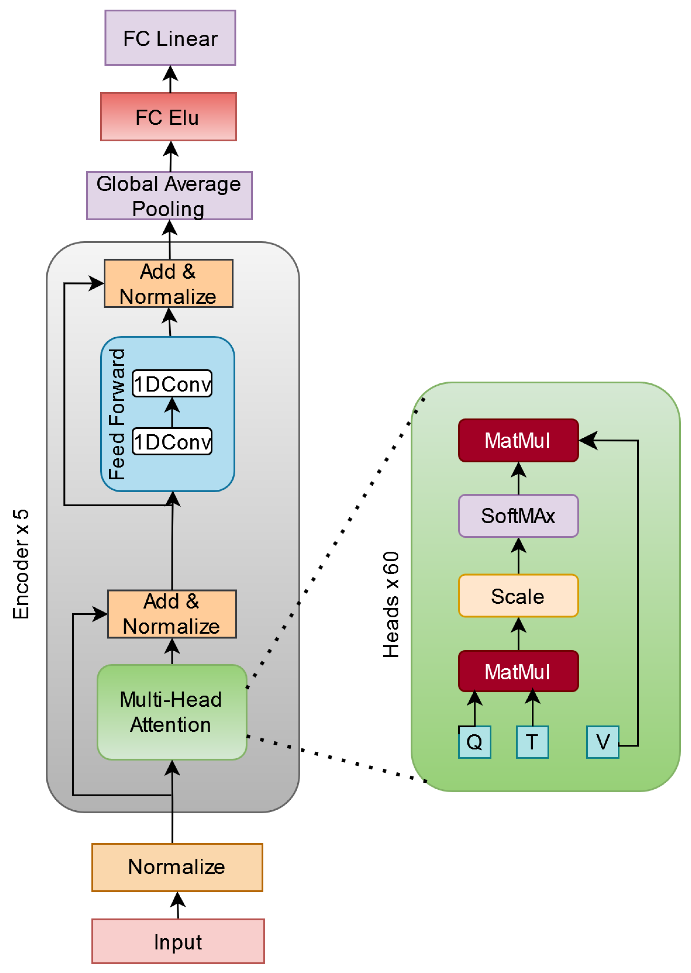
Initially, the EXPERT model receives input data in the form of historical currency exchange rate values. Each input sequence represents historical exchange rates for a specific currency pair over a period of time. This input data is passed through an embedding layer, converting it into numerical vectors that the model can understand. The embedded input sequences are then passed through multiple transformer encoder layers, each consisting of multi head self attention mechanisms 1 and feed forward neural networks. After processing through these layers, the model generates output sequences.
The model is trained using historical currency financial data, adjusting its parameters to minimize the difference between its predictions and the actual data. Once the model is trained, it attempts to predict the next day’s closing price for the exchange rates mentioned in this paper.
The EXPERT architecture consists of the following components:
Figure 1.
Encoder based model architecture of EXPERT.
Embedding Layer
The embedding layer initiates with data normalization, a technique essential for stabilizing the training process by standardizing the input data. This is achieved using Layer Normalization, which normalizes the input data as follows:
where:
and is a small constant for numerical stability, and d is the dimension of the input features.
Encoder
The core of the EXPERT model is the encoder, which takes the input time series data and transforms it into a sequence of hidden states. This is done using a stack of encoder blocks. Each encoder block consists of two sublayers:
- Self attention layer: This layer allows the model to learn long range dependencies in the input data. A key part of this is the residual connection, which ensures that the input is passed forward while also allowing the model to learn relationships:
- Feed forward network: The feed forward network allows the model to learn non linear relationships between the input data and the output value. Mathematically, this is computed as:where , , , , and
d represents the dimensionality of the input and output of the FFN. It is typically the hidden size of the input sequence after processing by the encoder. It remains consistent throughout the architecture, f represents the dimensionality of the intermediate layer within the FFN. This is usually larger than d, providing the network with a greater capacity to model complex transformations.
Global Average Pooling
The global average pooling layer takes the sequence of hidden states from the encoder and converts it into a single vector. This vector represents the overall trend of the input time series data. The operation is defined as:
where n is the sequence length. The pooling operation compresses the sequence, allowing the model to focus on global trends.
Multilayer Perceptron (MLP)
The MLP takes the output of the global average pooling layer as input and predicts the output value. Each layer of the MLP performs the following transformation:
where and are the weights and biases, and ELU is the activation function applied at each layer.
Output Layer
The final output layer applies a linear transformation to predict the output value. This is represented by the following equation:
where and are the weights and biases of the output layer.
Encoder Based Model - Hyperparameter Values
The optimization of the benchmarks in this study was focused on hyperparameter tuning to improve model performance. Key hyperparameters considered for optimization included the number of attention heads, feed forward network dimension, the number of transformer blocks, learning rate scheduling, and dropout rates. These parameters were chosen due to their significant impact on the performance of transformer based models.
The corresponding value range for each hyperparameter were delineated as follows:
- Number of attention heads: Tested values ranged from 2 to 60 heads.
- Feedforward network dimension: It varied between 128 and 1024 units.
- Number of transformer blocks: The number of transformer layers varied between 2 to 7 blocks.
- Learning rate: A custom learning rate scheduler was implemented to progressively increase the learning rate during the initial warm up period (30 epochs), followed by gradual decay over 100 epochs. The base learning rate was set at , with a minimum learning rate of .
- Dropout rates: Applied to both the transformer layers and the fully connected layers, dropout rates ranged between 0.1 and 0.48 to prevent overfitting.
The search for optimal hyperparameters was carried out using a combination of grid search and manual tuning, informed by early experimental results and prior knowledge. Grid search was employed for discrete parameters such as the number of attention heads and transformer blocks, while a more manual approach was applied for parameters like learning rate and dropout, as these often required finer control during training iterations. Additionally, we tested various training dataset ranges, from 75% to 96%, with the remaining portion of the data reserved for testing. This allowed us to assess the model’s performance across different training set sizes.
The implementation leveraged TensorFlow and Keras libraries for deep learning, with specific reliance on Keras’ Sequential API and the MultiHeadAttention and Conv1D layers for constructing EXPERT model architecture. The MinMaxScaler from scikit-learn was used for feature scaling, and early stopping with learning rate scheduling was implemented using Keras callbacks to prevent overfitting and optimize the learning process.
Table 2 presents the hyperparameter configurations used for different currency pairs in our EXPERT models. While the general structure of the model remains consistent across different setups, key parameters such as the number of attention heads, feedforward dimension, and batch size vary depending on the specific dataset. The proposed architecture consists of multiple stacked transformer blocks, each incorporating a self attention mechanism with varying head sizes and feedforward layers. The MLP layer contains 256 units for all currency pairs. To prevent overfitting, dropout is applied to both the MLP layers and the encoder blocks, with an MLP dropout rate varying per experiment, while the encoder dropout remains fixed at 0.1 for all cases. A global average pooling layer aggregates sequence level representations, which are subsequently passed through fully connected layers to generate the final forecasting output. The model is trained using adaptive optimizers, such as ADAM and ADAMW, with batch sizes optimized for each currency pair to ensure robust performance.
5. Alternative Forecasting Models
5.1. Linear Regression
The Linear Regression model is one of the most fundamental and widely utilized statistical instruments for predictive analysis. It operates by establishing a linear relationship between input features and the target variable. Essentially, the model fits a straight line to the data points such that the sum of the squared deviations between the observed and the predicted values is minimized. Linear Regression is particularly advantageous for revealing the relationship between two continuous variables and making predictions based on this correlation.
Notwithstanding its simplicity, Linear Regression is frequently the preferred option for regression tasks. The model’s analytical form is particularly suited for economic and financial interpretation and for deriving policy implications. Its low computational cost renders it ideal for large datasets or systems with limited computing power, with results being immediate. The principal limitation of linear regression is its assumption of a linear relationship, which may not precisely encapsulate complex real world phenomena. Moreover, outliers can significantly affect the model’s performance.
5.2. Random Forest
Random Forest constitutes a versatile and extensively utilized machine learning framework that combines the predictions of multiple decision trees to enhance accuracy introduced by Breiman [11]. By training on randomized subsets of data and incorporating stochasticity at each decision node, it overcomes the limitations inherent in solitary decision trees and mitigates overfitting. This adaptable model is effective for both classification and regression tasks, rendering it a favored option across diverse machine learning applications. During the implementation of the Random Forest Regressor model, the emphasis is placed on optimizing two crucial parameters: maximum depth and minimum sample split. In our experiments, we examined maximum depths reaching up to 50 and minimum sample split values of 5 or 10. To ascertain the optimal parameter combination (maximum depth, minimum sample split), grid search and 5 fold cross validation were employed.
The main concept of Random Forest, which involves integrating numerous regressors into a unified system, renders it an ideal and resilient choice capable of effectively managing noise and outliers. Typically, the model averts overfitting and delivers precise predictions. A notable disadvantage of Random Forest is its inability to provide an interpretable model representation. Moreover, as the number of regressors within the forest escalates, the computational cost correspondingly increases at a rapid pace.
5.3. Stochastic Gradient Descent
The Stochastic Gradient Descent (SGD) Regressor is a widely used optimization algorithm employed in the training of linear regression models [12]. Its operational mechanism involves the iterative update of model parameters in a direction that reduces the error between predicted and actual values, all while employing a subset of the training data in each iteration. This attribute renders it computationally efficient and well suited for large datasets. The algorithm based on gradient descent possesses the ability to traverse local minima, facilitating the attainment of a global minimum.
The SGD Regressor is exceptionally useful for large scale and sparse datasets, providing adaptability concerning the choice of the loss function and regularization methods, thereby establishing itself as a good instrument for regression tasks in the field of machine learning. Conversely, SGD exhibits suboptimal performance in noisy environments and demands meticulous adjustment of hyperparameters, along with a pronounced sensitivity to feature scaling.
5.4. XGBoost
The XGBoost Regressor represents a sophisticated enhancement of the gradient boosting algorithm, explicitly engineered for optimal speed and performance introduced by Chen & Guestrin [13]. XGBoost, which stands for eXtreme Gradient Boosting, has achieved significant acclaim within machine learning competitions and practical applications, attributed to its exceptional accuracy and efficiency. The model functions through the sequential augmentation of predictors while minimizing errors via gradient descent optimization. The XGBoost Regressor offers numerous benefits, such as its capacity for handling missing data, implementing regularization, and facilitating parallel processing, thereby making it an ideal option for regression tasks where precision and computational speed are paramount. However, it should be noted that the model performs poorly with sparse and unstructured data.
5.5. Bagging Regression
The Bagging Regression model, introduced by Breiman [14], abbreviated from Bootstrap Aggregating, represents an ensemble learning approach designed to enhance the stability and accuracy of regression models. This technique operates by training multiple base regressors on random subsets of the training data, with replacement. The potential base regressors include a variety of regression algorithms, such as Decision Trees, Support Vector Machines, or Linear Regression. During the prediction phase, the Bagging Regression model synthesizes the predictions of all base regressors, typically by averaging, to arrive at the final output. By mitigating variance and reducing overfitting, the Bagging Regression method significantly enhances overall predictive performance, thus establishing itself as a good method for regression within the field of machine learning. In our study, a specific application of the Bagging Regressor was implemented, employing 100 base regressors as part of the ensemble learning process.
Bagging regression is a low variance approach that yields robust models. It is capable of managing high dimensional datasets and mitigating overfitting. The training process can be executed through parallel processing, which reduces computational time; nonetheless, the computational cost can be substantial, as it correlates with the number of constituent models. The effectiveness of the model is enhanced when the base models exhibit diversity; however, this diversity obstructs the possibility of producing models that are easily interpretable.
5.6. Long Short Term Memory
Long Short Term Memory (LSTM) constitutes a subset of recurrent neural network (RNN) architectures that are specifically designed to address the vanishing gradient problem associated with traditional RNNs, and are capable of capturing long term dependencies within sequential data. The model was introduced by Hochreiter & Schmidhuber[15]. In contrast to standard RNNs, LSTMs exhibit a more elaborate architecture, marked by a persistent cell state that spans the entire sequence, and three gating mechanisms: the input gate, the forget gate, and the output gate. The input gate manages the access of new information into the cell state, the forget gate determines which information should be eliminated from the cell state, and the output gate governs the information to be emitted based on the cell state. This sophisticated gating mechanism endows LSTMs with the capacity to effectively maintain and utilize long term dependencies within sequential data, thus making them highly applicable for an array of tasks including time series forecasting, natural language processing, and speech recognition.
The primary benefit of LSTM networks lies in their capacity for long term dependency, enabling the model to retain information throughout the training phase over extended durations. Conversely, its complexity exceeds that of preceding models, rendering it susceptible to overfitting if not accurately trained and validated.
6. Evaluation Metrics
To assess the performance of the forecasting models created for this paper, we used the Mean Absolute Percentage Error (MAPE), the Mean Absolute Error (MAE) and the Mean Squared Error (MSE) metrics.
MAPE is the average of the absolute percentage differences between the actual and predicted values, and it is calculated as follows:
The MAPE is easy to understand because it expresses the accuracy of the model as a simple percentage. In addition, MAPE is scale invariant, making it optimal for comparing the different exchange rates in our data set. The main shortcoming of the MAPE metric is that it is sensitive to values close to zero.
MAE is the average of the absolute errors (the differences between the actual and the predicted values), and is calculated as follows:
MAE is easy to implement and understand. However, MAE is not scale invariant and punishes large errors more than small ones, making it sensitive to outliers.
MSE is the average of the squared differences between the actual and predicted values. It is calculated as follows:
7. Model’s Performance
7.1. Next Day Forecasting
In this section, we assess the forecasting performance of the proposed EXPERT model against six alternative forecasting models, namely Linear Regression, Random Forests, SGD, XGB, Bagging Regression and LSTM on 9 exchange rates: EUR/USD, AUD/CAD, GBP/AUD, NZD/USD, USD/JPY, EUR/AUD, EUR/CAD, USD/MXN, BRL/USD, covering the dynamics of various currency pairs on the next day forecasting.
Table 3 showcase the efficacy of each forecasting model for every currency exchange rate. The bold values show the optimal model, and the underlined values show the second best one.
Upon analysis of the reported results, several key conclusions can be drawn: a) all methodologies demonstrate high levels of accuracy in their predictions, with MAPE values consistently below 1%, b) the MAE values align well with MAPE, enhancing confidence in the conclusions, and c) the proposed Transformer based EXPERT model consistently outperformed all other methodologies. However, in the BRL/USD pair, the LIN methodology exhibited a lower MAE compared to the EXPERT model, despite the latter maintaining superior overall performance with lower MAPE and MSE values. The forecasting accuracy of EXPERT as counted by the MAPE ranged from 0.449% in the case of the NZD/USD to 0.275% in the case of USD/JPY.
The LSTM model achieved the second best performance in most cases, including EUR/USD, AUD/CAD, EUR/AUD, GBP/AUD and USD/JPY. Linear regression (LIN) ranked second in exchange rate BRL/USD in terms of MAPE, achieving the second lowest MAPE value, and also ranked second in the USD/MXN exchange rate based on MAE and MSE. Additionally, other models like SGD and XGB occasionally demonstrated close competition across the datasets.
In Table 4 we present the relative performance gain using the EXPERT model over the second best forecasting model.
The forecasting accuracy gain achieved by the EXPERT model over the second best method ranges from 3.21% in the case of the OLS forecasting model for the BRL/USD exchange rate to 18.29% in the case of the LSTM model for the NZD/USD exchange rate.
Figure 2 and Figure 3 present a series of scatter plots comparing actual versus forecasted prices, offering a comprehensive visual assessment of the model’s predictive performance across different scenarios. These plots illustrate the degree of correlation between observed and predicted values, highlighting trends and potential discrepancies in the forecasts.
7.2. Longer Forecasting Horizon
To further assess the proposed EXPERT methodology, we tested its predicting power at multiple forecasting horizons ranging from two days up to fourteen days ahead for the EUR/USD currency pair.
Static Forecasting
Initially, a static forecasting scenario was examined wherein the independent variables were restricted to historical values up to the time instance t, while the target values remained . For each forecasting horizon, the EXPERT model was re-trained following the identical procedure applied for the next day forecast. For instance, when evaluating a forecasting horizon of +3, data up to time instance t were utilized during model training to predict the value observed at time instance .
Dynamic Forecasting
In the second scenario, we employed the next day forecasting model in a recursive manner to dynamically extend the forecasting horizon. In this approach, the independent variables were confined to historical values up to instance t. However, predicted values obtained in were utilized to make forecasts for , and similarly, predicted values in were used to anticipate , and so forth.
Table 5 shows the performance of the Static and the Dynamic Forecasting scenarios for various horizons.
As expected, the accuracy decreases as the forecasting horizon distance increases. However, the forecasting error is acceptable even for the fourteen days ahead forecasting model, reaching just 3.5%. The performance of the dynamic forecast is more accurate than the static forecast for every forecasting horizon, yielding very close to the static forecast after 14 days.
7.3. Multiple Comparisons with the Best Evaluation
Hsu’s MCB method [28] is a multiple comparison approach to identify factor levels that are best, insignificantly different, or significantly different from the best (the best is defined as either the highest or lowest mean). When employed with a trained model, it provides precise analysis of level mean differences. It constructs a confidence interval for the difference between each level mean and the best among others.
In this section, we aim to evaluate the performance reliability of the EXPERT model across distinct parts of the EUR/USD dataset. To achieve this, five discrete samples, each comprising 20 data points, were extracted. These samples are chosen to reflect different market conditions, allowing the evaluator to determine how well the EXPERT model performs under varying market scenarios.
- Sample 1: December 28, 2018, to January 24, 2019.
- Sample 2: May 2, 2019, to May 29, 2019.
- Sample 3: February 6, 2020, to March 4, 2020.
- Sample 4: February 3, 2021, to March 2, 2021.
- Sample 5: January 5, 2022, to February 1, 2022.
The evaluation of the EXPERT model’s performance was conducted using the MAE between the predicted and the actual values:
where m is the sample size (in our case ) and k is the index of the first observation in the current sample.
To determine the statistical significance of performance differences across samples Hsu’s Multiple Comparisons with the Best (MCB) method was applied with an alpha value of 0.05. In our context, the "best" refers to the sample with the smallest mean, against which other samples are compared.
The differences between the mean of each period and the mean of the "best" period are used to calculate confidence intervals for each period. These intervals determine if the difference between each group and the best group is statistically significant or not according to the following rules shown in Table 6:
In our case, the smallest mean (the best case) is identified in the second sample; Results are shown in Table 7.
Our analysis employing MCB shows that the proposed model performed similarly to the best sample across different samples. This is a hint of consistency and uniformity in the results, underscoring the reliability of our findings. We can suggest that the EXPERT model will yield accurate, reliable, and equivalent outcomes across diverse scenarios.
8. Trading Scenario
To assess the practical applicability of the proposed model, we used it in the core of a trading strategy, which was subsequently tested on the EUR/USD currency pair from December 2018 to March 2022. The strategy driven by the model operates by a straightforward principle: it initiates a purchase when the forecasted price exceeds the current market price and initiates a sale when the forecasted price is lower than the market price. Such model driven strategies are prevalent in algorithmic trading and quantitative finance due to their simplicity and efficacy in capturing short term market trends. Prior research has shown that machine learning based forecasts can substantially enhance decision making in trading strategies [6,21]. The EXPERT model based trading strategy was compared against a simplistic buy and hold strategy and Random strategy. The buy and hold approach involves investing the initial capital into EUR/USD at the commencement and maintaining this investment without executing further trades. Its performance reflects the cumulative return that would occur if the investor does not trade. The Random strategy opens orders randomly without any criteria.
- Step 1:
-
Initial Conditions:
- The initial capital allocation (initial_cash) is set at $10,000, with no initial position to the EUR/USD currency pair (i.e., the number of contracts held is zero).
- Each iteration (trading day) evaluates whether the model’s prediction suggests a buy, sell or hold action.
- Step 2:
-
Trading Rules:
- Buy Signal: The strategy generates a buy signal when there is available cash in the investing portfolio and the model’s predicted price for the currency pair on a given day exceeds the previous day’s closing price. In this case, all available cash is allocated to purchase contracts.
- Sell Signal: A sell signal occurs when the portfolio contains currency contracts and the predicted price is less than the previous day’s closing price. The strategy responds by selling all held contracts, converting these positions back to cash. The return on investment is calculated by determining the relative difference in the exchange rate between the purchase price and the sale price, which generates a profit or loss.
-
Hold Signal: The strategy implicitly holds its current position in two scenarios:
- (a)
- After Buying: Once contracts are purchased, the strategy continues to hold them until a sell signal is triggered, regardless of further predicted price increases. There is no incremental buying or position scaling.
- (b)
- With Cash: If no buy signal is triggered (i.e., the prediction indicates a price decrease or no significant change), the strategy holds cash and waits for a favorable buy signal.
This decision making framework reflects a simple, rule based "all in, all out" approach, where the entire capital is either fully invested in contracts or held entirely in cash, depending on the model’s prediction. Such an approach aligns with similar strategies discussed in quantitative finance and algorithmic trading research [16,17]. - Step 3:
-
Portfolio Value Evaluation:
-
The performance of the trading strategy is evaluated based on the profit and loss achieved in each executed trade. The outcome of a trade is determined by comparing the exit price, i.e., the price at which the currency pair is sold, to the entry price, i.e., the price at which the currency pair is bought.A trade is classified as profitable if the exit price is higher than the entry price and as a loss if the exit price is lower than the entry price. The profit and loss for a trade is calculated as follows:At each step, the portfolio value is computed based on the state of the portfolio, which can be in one of two mutually exclusive conditions:
- (a)
- All Cash: If no contracts are held, the portfolio value equals the cash balance.
- (b)
- All Contracts: If a position is held, the portfolio value equals the market value of the position.
-
- Step 4:
-
Comparison Strategies:
- Buy and Hold Strategy: The buy and hold approach invests the initial capital in the currency at the start and holds it without further trades. Its performance reflects the cumulative return if the investor had not traded based on predictive signals.
- Random Strategy: The Random Strategy generates buy, sell, or hold signals randomly, without relying on any price data or indicators. The execution follows predefined conditions buying only when no position is held and selling only when a position is available. Portfolio value, winning and losing trades, and annualized returns are tracked to compare performance against model driven approache.
- Step 5:
-
Performance Metrics:
- Annualized Returns: To gauge each strategy’s effectiveness, we compute annualized returns based on cumulative returns and the number of trading days (assuming 252 trading days per year). The annualized return metric provides insight into the average yearly performance of each approach. The trading scenario has been tested for the period from December 2018 to March 2022.
Table 8.
Trading Performance of Different Strategies
| Strategy | Performance |
|---|---|
| EXPERT | 2.36% |
| Buy-and-Hold | -0.77% |
| Random | -2.34% |
8.1. Strategy Performance Analysis
The performance analysis of the tested trading strategies reveals that the EXPERT Strategy achieved the highest annualized return, yielding a profit of 2.36%. This result notably surpasses the other strategies, each of which underperformed over the evaluation period. Specifically, the Buy and Hold Strategy closely trailed at -0.77% while the Random Strategy resulted in an annualized return of -2.34%, demonstrating that purely random trading decisions led to a net loss rather than serving as a neutral benchmark. These findings underscore the superior predictive capability of the EXPERT model in optimizing trading decisions compared to traditional or stochastic approaches.
9. Conclusion
This paper is a study evaluating the ability of a Transformer based model called EXPERT to forecast exchange rates on a daily basis. The study compares the performance of the EXPERT model to that of six other widely used forecasting models: Linear Regression, Random Forests, Stochastic Gradient Descent, XGBoost, Bagging Regression, and LSTM. The dataset employed in the study encompasses a temporal span from 1999 to 2022 and comprises 9 currency pairs exhibiting diverse characteristics. The models were evaluated using the MAPE, MAE and MSE metric in forecasting the subsequent day’s closing price.
- The EXPERT model demonstrated superior performance compared to the other forecasting models in all cases, indicating its efficacy in predicting exchange rates on a daily basis. This underscores the efficacy of the attention mechanism and the capacity of the EXPERT model to capture long term dependencies in financial time series data.
- The precision of the EXPERT model in the 14 day ahead forecasting setup for the EUR/USD exchange rate demonstrates its potential for longer term predictions. This is of particular value to traders, investors, and businesses that require the ability to plan and execute international transactions and manage foreign currency exposure.
- The presented methodology contributes to the ongoing discussion on the use of ML and, in particular the branch of ML that employs recurrent mechanisms, such as the GRU and the LSTM, to capture complex patterns and dependencies in financial time series. It demonstrates that the Transformer paradigm can also be employed to address the problem of time series forecasting.
Overall, the study demonstrates the effectiveness of the EXPERT model for exchange rate forecasting and highlights the potential of advanced computational techniques in this field. The findings have implications for traders, investors, businesses, and policymakers who rely on accurate exchange rate forecasts for decision making and risk management.
Author Contributions
Conceptualization, E.B., K.D. and K.G.; methodology, E.B., T.P. and K.D.; software, E.B.; validation, E.B.; formal analysis, E.B., K.D. and T.P.; investigation, E.B.; resources, E.B.; data curation, E.B.; writing—original draft preparation, E.B.; writing—review and editing, E.B., K.D. and T.P.; visualization, E.B.; supervision, T.P., K.D. and K.G.; project administration, K.G.; funding acquisition, No. All authors have read and agreed to the published version of the manuscript.
Funding
This research received no external funding.
Data Availability Statement
Restrictions apply to the availability of these data. Data were obtained from the MetaTrader platform (MetaQuotes Ltd.) via the Alpari demo server. The data are available from the authors upon request or by registering for a free demo account with Alpari at https://alpari.com.
Acknowledgments
During the preparation of this manuscript, the authors used ChatGPT (OpenAI, GPT-4) to assist with grammar and language editing. The authors have reviewed and edited the output and take full responsibility for the content of this publication.
Conflicts of Interest
The authors declare no conflicts of interest.
References
- Huang, J.; Chai, J.; Cho, S. Deep learning in finance and banking: A literature review and classification. Front. Bus. Res. China 2020, 14.
- Wood, K.; Giegerich, S.; Roberts, S.; Zohren, S. Trading with the Momentum Transformer: An intelligent and interpretable architecture. arXiv 2022, arXiv:2112.08534. Available online: https://arxiv.org/abs/2112.08534.
- Gradzki, P.; Wójcik, P. Is attention all you need for intraday Forex trading? Expert Syst. 2023, 41.
- Fischer, T.; Sterling, M.; Lessmann, S. Fx-spot predictions with state-of-the-art transformer and time embeddings. Expert Syst. Appl. 2024, 249, 123538.
- Kantoutsis, K.; Mavrogianni, A.; Theodorakatos, N. Transformers in High-Frequency Trading. J. Phys. Conf. Ser. 2024, 2701, 012134.
- Sezer, O.; Gudelek, M.; Ozbayoglu, A. Financial time series forecasting with deep learning: A systematic literature review: 2005–2019. Appl. Soft Comput. 2020, 90, 106181.
- Ryll, L.; Seidens, S. Evaluating the performance of machine learning algorithms in financial market forecasting: A comprehensive survey. arXiv 2019, arXiv:1906.07786. Available online: http://arxiv.org/abs/1906.07786.
- Panda, M.; Panda, S.; Pattnaik, P. Exchange rate prediction using ANN and deep learning methodologies: A systematic review. Proceedings of the 2020 Indo–Taiwan 2nd International Conference on Computing, Analytics and Networks (Indo-Taiwan ICAN), 2020, 1–6.
- Fletcher, T. Machine learning for financial market prediction. Doctoral Thesis, University College London, 2012.
- Islam, M.; Hossain, E.; Rahman, A.; Hossain, M.; Andersson, K. A review on recent advancements in FOREX currency prediction. Algorithms 2020, 13, 186.
- Breiman, L. Random forests. Mach. Learn. 2001, 45(1), 5–32.
- Chen, X.; Lee, J. D.; Tong, X. T.; Zhang, Y. Statistical inference for model parameters in stochastic gradient descent. Ann. Stat. 2020, 48(1), 251–273.
- Chen, T.; Guestrin, C. XGBoost: A scalable tree boosting system. In Proceedings of the 22nd ACM SIGKDD International Conference on Knowledge Discovery and Data Mining; ACM: New York, NY, USA, 2016; pp. 785–794.
- Breiman, L. Bagging predictors. Mach. Learn. 1996, 24(2), 123–140.
- Hochreiter, S.; Schmidhuber, J. Long short-term memory. Neural Comput. 1997, 9(8), 1735–1780.
- Avellaneda, M.; Stoikov, S. High-frequency trading in a limit order book. Quant. Finance 2008, 8(3), 217–224.
- Krauss, C.; Do, X. A.; Huck, N. Deep neural networks, gradient-boosted trees, random forests: Statistical arbitrage on the S&P 500. Eur. J. Oper. Res. 2017, 259(2), 689–702.
- Qi, L.; Khushi, M.; Poon, J. Event-driven LSTM for Forex price prediction. In Proceedings of the 2020 IEEE Asia-Pacific Conference on Computer Science and Data Engineering (CSDE); IEEE: Sydney, Australia, 2020.
- Islam, M.; Hossain, E. Foreign exchange currency rate prediction using a GRU-LSTM hybrid network. Soft Comput. Lett. 2021, 3.
- Goncu, A. Prediction of exchange rates with machine learning. In Proceedings of the International Conference on Artificial Intelligence, Information Processing and Cloud Computing; 2019.
- Hiransha, M. A.; Al-Khasawneh, M. A.; Khan, S. U. R.; Khan, Z. Stock market trend prediction using deep learning approach. Comput. Econ. 2018, 53(1), 123–135.
- Nelson, B. Time series analysis using autoregressive integrated moving average (ARIMA) models. Acad. Emerg. Med. 1998, 5, 739–744.
- Benjamin, M.; Rigby, R.; Stasinopoulos, D. Generalized autoregressive moving average models. J. Am. Stat. Assoc. 2003, 98, 214–223.
- Freeman, J.; Williams, J.; Lin, T. Vector autoregression and the study of politics. Am. J. Polit. Sci. 1989, 33, 842–875.
- Wu, N.; Green, B.; Ben, X.; O’Banion, S. Deep transformer models for time series forecasting: The influenza prevalence case. arXiv 2020, arXiv:2001.08317. Available online: http://arxiv.org/abs/2001.08317.
- Liu, J.; Liu, X.; Lin, H.; Xu, B.; Ren, Y.; Diao, Y.; Yang, L. Transformer-based capsule network for stock movements prediction. In Proceedings of the First Workshop on Financial Technology and Natural Language Processing; 2019; pp. 66–73.
- Vargas, M. R.; Anjos, C. E. M. D.; Bichara, G. L. G.; Evsukoff, A. G. Deep learning for stock market prediction using technical indicators and financial news articles. In Proceedings of the International Joint Conference on Neural Networks (IJCNN); IEEE: Rio de Janeiro, Brazil, 2018. [CrossRef]
- Hsu, J. C. Multiple Comparisons, Theory and Methods; Chapman & Hall/CRC: Boca Raton, FL, USA, 1996.
- Vaswani, A.; Shazeer, N.; Parmar, N.; Uszkoreit, J.; Jones, L.; Gomez, A. N.; Kaiser, L.; Polosukhin, I. Attention is all you need. In Advances in Neural Information Processing Systems; Curran Associates, Inc.: Red Hook, NY, USA, 2017.
| 1 | "Self Attention" refers to the mechanism that allows the model to weigh the importance of different elements in the input sequence when computing a representation of that sequence. Each element can attend to other elements to capture dependencies and contextual relationships within the sequence."Multi head" indicates that the self attention mechanism is executed multiple times (in parallel but independently) with different sets of learned parameters (heads). Each head has access to different representation subspaces, allowing the model to capture diverse patterns or relationships in the data. The results from these multiple heads are then concatenated and combined to form a comprehensive representation of the input sequence. |
Figure 2.
Performance of the EXPERT Model in Predicting Out of Sample currency prices (Actual vs. Predicted) (part A)
Figure 2.
Performance of the EXPERT Model in Predicting Out of Sample currency prices (Actual vs. Predicted) (part A)
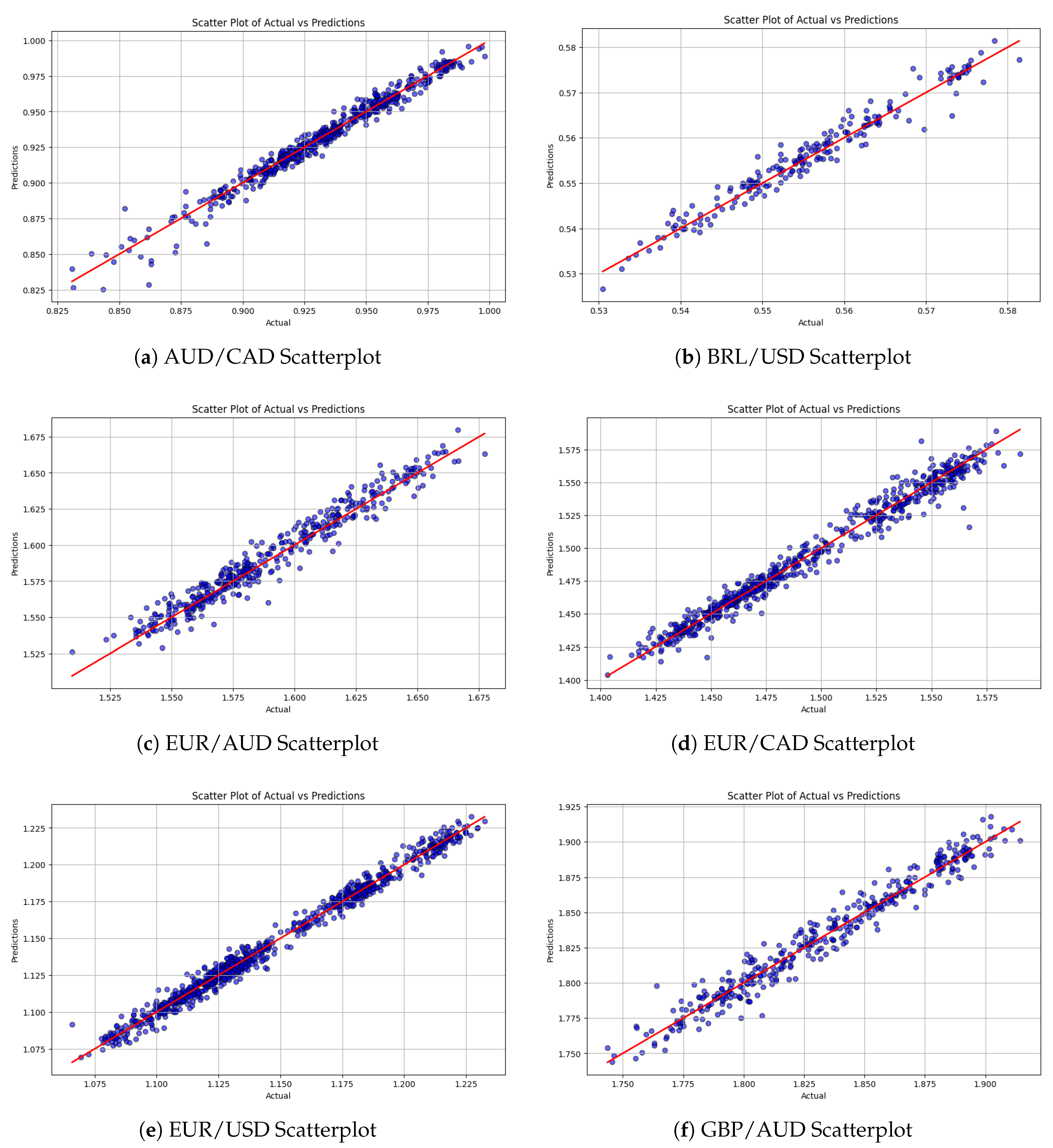
Figure 3.
Performance of the EXPERT Model in Predicting Out of Sample currency prices (Actual vs. Predicted) (part B)
Figure 3.
Performance of the EXPERT Model in Predicting Out of Sample currency prices (Actual vs. Predicted) (part B)
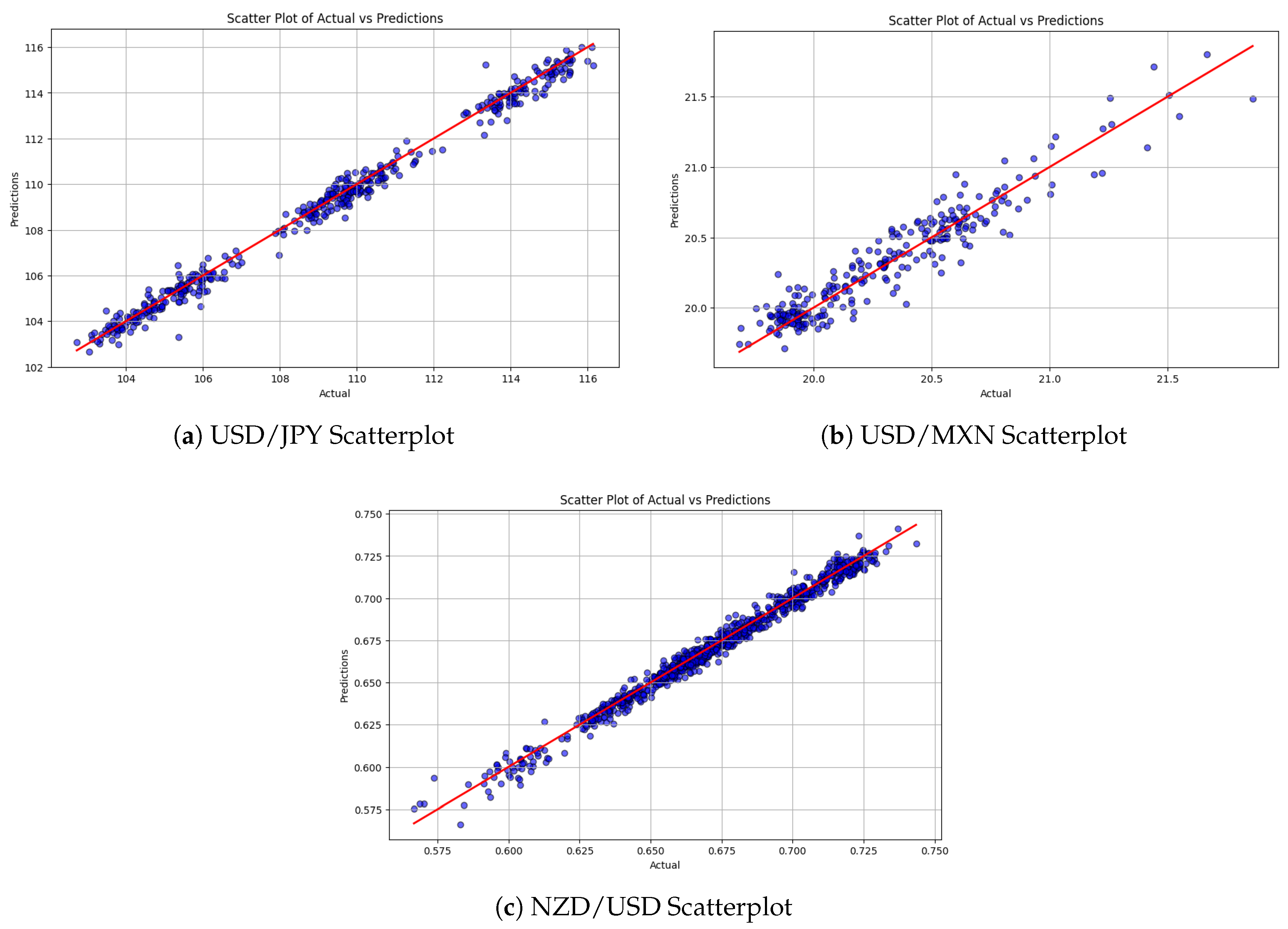
Table 2.
Hyperparameter configurations for different currency pairs in the EXPERT model.
| Currency Pair | Lag | Optimizer | Batch Size | Head Size | Heads | FF Dim | Blocks | MLP Dropout |
|---|---|---|---|---|---|---|---|---|
| AUDCAD | 20 | ADAM | 20 | 46 | 60 | 256 | 5 | 0.25 |
| EURUSD | 8 | ADAMW | 18 | 19 | 34 | 512 | 2 | 0.48 |
| EURAUD | 9 | ADAM | 20 | 46 | 60 | 256 | 5 | 0.25 |
| EURCAD | 11 | ADAMW | 27 | 105 | 13 | 827 | 6 | 0.28 |
| GBPAUD | 20 | ADAM | 20 | 46 | 60 | 256 | 5 | 0.25 |
| NZDUSD | 13 | ADAMW | 17 | 121 | 2 | 1024 | 7 | 0.34 |
| USDJPY | 20 | ADAM | 20 | 46 | 60 | 256 | 5 | 0.2 |
| USDMXN | 9 | ADAM | 20 | 46 | 60 | 256 | 5 | 0.2 |
| BRLUSD | 7 | ADAM | 20 | 46 | 60 | 256 | 5 | 0.2 |
* FF Dim column represents the Feedforward Dimension.
Table 3.
Forecasting performance of each model
| EUR/USD | AUD/CAD | EUR/AUD | |||||||
|---|---|---|---|---|---|---|---|---|---|
| Model | MAPE | MAE | MSE | MAPE | MAE | MSE | MAPE | MAE | MSE |
| LIN | 0.440 | 0.528 | 0.006 | 0.443 | 0.414 | 0.004 | 0.448 | 0.696 | 0.010 |
| SGD | 0.485 | 0.578 | 0.007 | 0.446 | 0.417 | 0.004 | 0.485 | 0.750 | 0.011 |
| XGB | 0.483 | 0.580 | 0.007 | 0.477 | 0.445 | 0.005 | 0.492 | 0.759 | 0.012 |
| BGR | 0.485 | 0.581 | 0.007 | 0.491 | 0.459 | 0.005 | 0.515 | 0.800 | 0.013 |
| RF | 0.477 | 0.572 | 0.007 | 0.480 | 0.449 | 0.005 | 0.511 | 0.793 | 0.013 |
| LSTM | 0.322 | 0.369 | 0.003 | 0.398 | 0.368 | 0.003 | 0.398 | 0.650 | 0.008 |
| EXPERT | 0.298 | 0.341 | 0.002 | 0.328 | 0.304 | 0.002 | 0.362 | 0.576 | 0.005 |
| EUR/CAD | GBP/AUD | NZD/USD | |||||||
| Model | MAPE | MAE | MSE | MAPE | MAE | MSE | MAPE | MAE | MSE |
| LIN | 0.418 | 0.613 | 0.007 | 0.459 | 0.838 | 0.014 | 0.579 | 0.384 | 0.003 |
| SGD | 0.431 | 0.631 | 0.007 | 0.489 | 0.894 | 0.017 | 0.616 | 0.410 | 0.003 |
| XGB | 0.432 | 0.633 | 0.007 | 0.481 | 0.880 | 0.016 | 0.627 | 0.416 | 0.003 |
| BGR | 0.444 | 0.653 | 0.008 | 0.505 | 0.925 | 0.018 | 0.634 | 0.421 | 0.003 |
| RF | 0.441 | 0.648 | 0.007 | 0.497 | 0.908 | 0.017 | 0.626 | 0.416 | 0.003 |
| LSTM | 0.347 | 0.520 | 0.005 | 0.387 | 0.717 | 0.009 | 0.504 | 0.336 | 0.002 |
| EXPERT | 0.342 | 0.512 | 0.005 | 0.337 | 0.616 | 0.007 | 0.449 | 0.301 | 0.001 |
| Model | MAPE | MAE | MSE | MAPE | MAE | MSE | MAPE | MAE | MSE |
| USD/JPY | USD/MXN | BRL/USD | |||||||
| Model | MAPE | MAE | MSE | MAPE | MAE | MSE | MAPE | MAE | MSE |
| LIN | 0.437 | 46.89 | 42.21 | 0.593 | 9.662 | 2.198 | 0.311 | 0.122 | 0.058 |
| SGD | 0.448 | 48.08 | 45.24 | 0.632 | 10.429 | 2.486 | 0.519 | 0.208 | 0.091 |
| XGB | 0.477 | 50.98 | 48.42 | 0.665 | 10.693 | 2.515 | 0.454 | 0.179 | 0.077 |
| BGR | 0.485 | 52.00 | 51.27 | 0.633 | 10.329 | 2.243 | 0.474 | 0.188 | 0.102 |
| RF | 0.476 | 50.99 | 49.74 | 0.630 | 10.293 | 2.258 | 0.449 | 0.178 | 0.090 |
| LSTM | 0.315 | 34.30 | 24.16 | 0.574 | 11.74 | 2.450 | 0.327 | 0.182 | 0.056 |
| EXPERT | 0.275 | 29.83 | 15.80 | 0.469 | 9.566 | 1.552 | 0.310 | 0.173 | 0.051 |
* MAPE, MAE and MSE are counted as a percentage.
Table 4.
The relative gain of the EXPERT versus the second best methodology
| Currency Pair | 2nd best model | Relative MAPE Gain (%) |
|---|---|---|
| EUR/USD | LSTM | 7.45 |
| AUD/CAD | LSTM | 1.44 |
| EUR/AUD | LSTM | 12.70 |
| EUR/CAD | LSTM | 17.59 |
| GBP/AUD | LSTM | 12.92 |
| NZD/USD | LSTM | 18.29 |
| USD/JPY | LSTM | 9.05 |
| USD/MXN | LSTM | 10.91 |
| BRL/USD | OLS | 3.21 |
Table 5.
Static and Dynamic Forecasting Performance for various Horizons
| Static Forecasting | Dynamic Forecasting | |
| Forecasting Horizon | MAPE | MAPE |
| 1 | 0.298 | 0.298 |
| 2 | 1.674 | 0.975 |
| 3 | 1.989 | 1.060 |
| 4 | 2.065 | 1.255 |
| 5 | 2.153 | 1.664 |
| 6 | 2.200 | 1.875 |
| 7 | 2.282 | 1.996 |
| 8 | 2.406 | 2.229 |
| 9 | 2.448 | 2.336 |
| 10 | 2.731 | 2.395 |
| 11 | 3.008 | 2.477 |
| 12 | 3.178 | 2.861 |
| 13 | 3.336 | 3.220 |
| 14 | 3.547 | 3.501 |
* MAPE is counted as a percentage.
Table 6.
Evaluation Criteria for Hsu’s Multiple Comparisons with the Best
| Smallest is Best | |
|---|---|
| No difference from best | |
| Worse than best | |
| Better than other groups |
Table 7.
D-TEST (Min) Evaluation Results
| Group | Mean | Center | Lower | Upper | Evaluation |
|---|---|---|---|---|---|
| Sample 1 | 0.0045 | 0.0028 | -0.0002 | 0.0058 | No difference from best |
| Sample 2 | 0.0017 | -0.0018 | -0.0080 | 0.0043 | No difference from best |
| Sample 3 | 0.0029 | 0.0012 | -0.0050 | 0.0074 | No difference from best |
| Sample 4 | 0.0034 | 0.0017 | -0.0045 | 0.0079 | No difference from best |
| Sample 5 | 0.0040 | 0.0023 | -0.0039 | 0.0085 | No difference from best |
Disclaimer/Publisher’s Note: The statements, opinions and data contained in all publications are solely those of the individual author(s) and contributor(s) and not of MDPI and/or the editor(s). MDPI and/or the editor(s) disclaim responsibility for any injury to people or property resulting from any ideas, methods, instructions or products referred to in the content. |
© 2025 by the authors. Licensee MDPI, Basel, Switzerland. This article is an open access article distributed under the terms and conditions of the Creative Commons Attribution (CC BY) license (http://creativecommons.org/licenses/by/4.0/).
Copyright: This open access article is published under a Creative Commons CC BY 4.0 license, which permit the free download, distribution, and reuse, provided that the author and preprint are cited in any reuse.


