Submitted:
07 September 2025
Posted:
08 September 2025
You are already at the latest version
Abstract
Humans learn new tasks without forgetting, but neural networks suffer catastrophic forgetting when trained sequentially.
Dynamic expandable networks attempt to address this by assigning each task its own feature extractor and freezing previous ones to preserve past knowledge.
While effective for retaining old tasks, this design leads to rapid parameter growth, and frozen extractors never adapt to future data, often producing irrelevant features that degrade later performance.
To overcome these limitations, we propose Task-Sharing Distillation (TSD), which reduces the number of extractors by allowing multiple tasks to share one extractor and consolidating them through distillation. We study two strategies: (1) Grouped Rolling Consolidation, which groups consecutive tasks and consolidates them into a shared extractor, and (2) Fixed-Size Pool with Similarity-Based Consolidation, where new tasks are merged into the most compatible extractor in a fixed pool according to prototype similarity.
Experiments on CIFAR-100 and ImageNet-100 show that TSD maintains strong performance across tasks, demonstrating that careful feature sharing is more effective than simply adding more extractors. The idea also has potential relevance for large language models, where continual and multi-domain adaptation face similar challenges of parameter growth and redundancy.
Keywords:
class incremental learning
; catastrophic forgetting
; knowledge distillation
1. Introduction
Humans learn new tasks without forgetting what they already know, but neural networks trained on sequential tasks typically suffer catastrophic forgetting [1], especially when access to old data is limited or only a few exemplars are available. Regularization-based methods add penalties that discourage changes to parameters deemed important for previous tasks. Rehearsal-based methods store a small subset of old examples for replay during new-task training. Knowledge distillation is also widely used; for example, iCaRL [2] freezes the model learned up to stage and uses it as a teacher to transfer old-task knowledge to the model at stage t. These approaches help, yet continual learning with a single shared backbone remains challenging.
Dynamic-network methods expand the model by assigning a dedicated feature extractor to each task. After training a task, its extractor is frozen, and a new extractor is allocated for the next task (see Figure 1, left). This prevents interference with parameters of previous tasks, but the number of extractors increases linearly with the number of tasks. For example, in methods such as DER, a full CNN backbone is added for every new task, so after M tasks the model contains M extractors. At test time, each input is processed by all extractors, and the resulting features are concatenated and fed into a global classifier. However, since early extractors are trained only on their original task data, their outputs are often irrelevant for later tasks. Consequently, concatenating features from all extractors introduces redundancy and noise, which reduces accuracy. For example, as shown in Table 1, on CIFAR-100, dividing 100 classes into 10 tasks requires 10 extractors and yields accuracy with DER. When the dataset is instead split into 20 tasks, the number of extractors doubles to 20, but the accuracy drops to . This demonstrates that increasing the number of extractors does not guarantee better performance, and excessive extractors can harm generalization by amplifying redundancy.
These observations highlight a key limitation: dedicating one extractor per task is inefficient. We therefore ask whether extractors can be shared across tasks to reduce their total number, mitigate interference from redundant extractors, and still preserve the benefits of dynamic networks. To this end, we propose Task Sharing Distillation(TSD), which reduces the number of extractors by allowing tasks to share them. We study two variants.
Grouped rolling consolidation. Consecutive tasks are grouped and merged to share a single extractor by distillation. For example, tasks 1–2 may share one extractor and tasks 3–4 another (see Figure 1, middle). The group size does not need to be fixed; different extractors may cover different numbers of tasks depending on the experimental setup.
Fixed-Size Pool with Similarity-Based Consolidation. We first set a maximum number of extractors. Early tasks each initialize a new extractor until this limit is reached. For every subsequent task, we train a temporary extractor and then merge it into the most compatible existing extractor through distillation. Compatibility is determined by prototype similarity: the new task’s feature prototypes are compared with those maintained by each existing extractor, and the task is merged into the extractor with the highest similarity. This strategy encourages feature reuse among related tasks while keeping the overall number of extractors bounded (see Figure 1, right).
To further ensure that different extractors maintain independent feature subspaces, we impose a feature distinctness constraint during training. When a new extractor is introduced, we add an explicit constraint that encourages its features to remain distinct from those of existing extractors. This constraint guides the new extractor toward representations that are discriminative with respect to previously learned subspaces, so that each extractor specializes in a subset of task subspaces and different subsets remain independent.
Compared with DER, our approach substantially reduces the number of backbone parameters. In particular, using only three extractors, our methods achieve higher accuracy than DER, which relies on ten extractors.
Although our experiments focus on vision tasks, the underlying idea is more general. Large language models (LLMs) are widely applied in continual and multi-domain settings, where assigning a separate adapter to each task similarly leads to parameter growth and redundancy. Our proposed Task-Sharing Distillation (TSD) offers a promising way to consolidate and share modules in such scenarios, highlighting its potential relevance for scaling LLMs efficiently.
Our main contributions are:
1. We analyze the relationship between the number of extractors and model performance. Increasing the number of extractors not only inflates parameters but also reduces generalization.
2. We propose Task-Sharing Distillation, which reduces the number of extractors by allowing tasks to share them and by consolidating multiple extractors through distillation. We present two practical strategies: grouped rolling consolidation, which groups consecutive tasks into a shared extractor, and Fixed-Size Pool with similarity based consolidation, which allocates a fixed number of extractors and assigns new tasks to the most similar one.
3. Our methods achieve superior accuracy and parameter efficiency compared with state-of-the-art methods such as DER. In particular, our methods outperform DER while using only three extractors, whereas DER requires ten.
2. Related Works
Incremental learning can be categorized into three main types [3,4]: task-incremental, domain-incremental, and class-incremental learning. In task-incremental learning, the model receives the task ID during evaluation and only classifies within the given task. Domain-incremental learning uses the same set of classes across tasks but with different domains [5,6]. Class-incremental learning assigns different classes to each task without providing the task ID at test time, so the model must classify across all classes.
To reduce forgetting, regularization methods such as EWC [1,7] constrain parameter updates based on their importance to previous tasks. Knowledge distillation methods [2,8,9,10,11,12,13] transfer knowledge from old feature extractors and exemplars, using distillation [14] to guide new models. Other works [15,16] address old-class forgetting caused by the imbalance between old and new samples. However, a single shared extractor remains limited. To improve capacity, AANets [17] combine stable and plastic blocks, and DualNet [18] incorporates complementary fast and slow learning systems [19]. GAN-based approaches [20,21] generate old samples to alleviate data scarcity, while auto-encoder based methods [22] learn class-specific subspaces for classification.
Dynamic network methods expand the architecture by adding feature extractors for new tasks. DER [23] assigns a new extractor to each task and freezes old ones. DyTox [24] introduces a transformer encoder-decoder with dynamic task tokens. TagFex [25] captures task-agnostic features and merge them with task-specific ones. FOSTER [26] learns new extractors inspired by gradient boosting and distills both old and new extractors into a unified network. MEMO [27] extend selected blocks instead of full extractors. SEED [28] employs a fixed number of feature extractors and models each class with a Gaussian distribution to select suitable extractors for learning new tasks.
3. Methodology
3.1. Problem Setup and Method Overview
In this section, we first define the class incremental learning task, then introduce dynamic-network-based approaches, and finally motivate our two methods that share feature extractors.
Class Incremental Learning Task. The goal of incremental learning is to train on a sequence of tasks and, after completing all tasks, maintain strong performance across all learned classes. Let the total number of tasks be T. For task , the dataset is with class set . The class sets are disjoint, i.e., for . Let denote the number of classes in task t. Each sample belongs to one of these classes.
Dynamic-Network Methods. Traditional incremental learning often uses a single backbone for all tasks, which risks severe forgetting. Dynamic-network methods address this by assigning a dedicated feature extractor to each task. We denote the extractor for task t as . A representative baseline, DER, trains on task t and then freezes its parameters. For the next task, a new extractor is introduced. At inference time, an input x is processed by all extractors, and their features are concatenated before being classified by a global head g:
Freezing prevents interference with past knowledge and improves performance compared with a single shared backbone. However, this design introduces two major issues. First, the number of parameters grows linearly with the number of tasks. Second, since learning is sequential, an extractor () never observes data from a future task , making its features irrelevant or even harmful for later tasks.
These limitations raise an important question: can we reduce the number of extractors while still retaining the benefits of dynamic networks? To address this, we introduce Task-Sharing Distillation (TSD), which progressively merges task knowledge into shared extractors through distillation. Building on TSD, our two methods, Grouped Rolling Consolidation and Fixed-Size Pool with Similarity-Based Consolidation, effectively control parameter growth, reduce redundancy, and maintain accuracy on both past and future tasks.
3.2. Grouped Rolling Consolidation (GRC)
Given T tasks, we partition them into groups , where each group contains a contiguous subset of tasks. The group size is not fixed in advance; different groups may cover different numbers of tasks depending on the schedule. After completing the first group , we freeze a consolidated extractor . For later groups, task-specific extractors are temporarily maintained, progressively merged by distillation into a rolling extractor , and finally frozen as at the end of the group. Importantly, denotes a single consolidated extractor obtained from tasks to t, not a concatenation of multiple extractors.
Training inside a group (, ).
Let be the first task in . All frozen extractors from previous groups are denoted by and remain fixed.
Case A (first task ). A new extractor and a temporary classifier head are instantiated. The classifier input concatenates frozen features with the new feature:
and the cross-entropy loss is
No consolidation is performed since there is only one new extractor in this group.
Case B (subsequent tasks ). For each new task, we instantiate an extractor and a temporary head . The current-group teacher feature is defined as
The full teacher feature is
and predicts over .
We first optimize and using the cross-entropy loss on :
After this step, and are frozen, and consolidation is applied.
Immediate consolidation at step t ().
We merge the current-group extractors into a rolling extractor with head , while keeping fixed. The student features are
Teacher and student logits are
.
Logit distillation with temperature is applied:
After optimization, the temporary teachers forming are discarded, and the rolling extractor is kept.
End of a group.
When the last task in is completed, the rolling extractor is frozen as the group extractor:
Thus, after K groups we obtain .
Inference.
After completing task , prediction uses the concatenation of all frozen group extractors and the current rolling extractor (if the group is not finished):
If t is the last task in , inference uses the frozen extractors only:
Worked example.
For instance, if tasks are grouped as , the procedure yields four frozen extractors .
3.3. Method 2: Fixed-Size Pool with Similarity-Based Consolidation
GRC controls parameter growth effectively, but it does not exploit task similarity. This raises a natural question: should similar tasks share extractors to further reduce redundancy? Since task similarity cannot be determined in advance under incremental learning, we adopt a simplified setting: we first allocate extractors to the initial N tasks, forming a fixed-size pool of N extractors. Subsequent tasks are then integrated by sharing with the most related extractor in this pool. The overall framework is illustrated in Figure 2.
Initialization with N extractors.
We predefine the number of available extractors as N. For the first N tasks, each task is assigned a new extractor and a classifier . During training, all previous extractors are frozen, and only and are updated. The classifier input concatenates features from all frozen extractors and the new one:
After training the N-th task, we retain the extractors .
Beyond N tasks: triggering consolidation.
When a new task arrives, we instantiate a temporary extractor and a classifier . The classifier takes as input the concatenation of features from all N frozen extractors and the new extractor :
The model is trained with cross-entropy over all classes from tasks 1 through t:
After training, the temporary extractor must be consolidated into one of the existing N extractors to keep the pool size fixed.
Similarity-based target selection.
For each class in the new task , we compute its prototype on extractor , with :
where denotes the set of samples from class .
For extractor and its own task , the prototype of class is
where denotes the exemplar set of class c from task .
The similarity score for class on is
Summing over all classes in task t, we obtain the task-to-extractor similarity
We select the extractor with the maximum similarity score as the consolidation target:
To avoid overusing a single extractor, we further enforce balanced selection among extractors. If an extractor is chosen for the current task, it is temporarily excluded from the next selection, and the consolidation target is chosen from the remaining extractors.
Consolidation training.
We copy the selected extractor and unfreeze it for optimization, while keeping the remaining extractors frozen. The teacher logits are produced by the classifier applied to the concatenation of features from all N frozen extractors and the frozen temporary extractor :
The student always maintains exactly N extractors. It replaces with its trainable copy and introduces a trainable head :
We minimize the distillation loss:
where is the temperature.
After optimization, we update and discard , ensuring that the extractor pool size remains N.
3.4. Training Objective
For each new task t, the learnable feature extractor and its task-specific classifier are optimized with a standard cross-entropy loss as Eq. 3, Eq. 6, Eq. 14 and Eq. 16. To further encourage feature space separation across extractors, we enhance the training of each newly added extractor using contrastive learning [33]. Specifically, memory samples from old tasks, processed by frozen extractors, are incorporated as additional negatives to guide toward a distinct representation space.
For a sample from the current task in the minibatch, the positive set consists of embeddings from augmented views of the same class, extracted by the current feature extractor . The negative set includes two sources: (i) embeddings from different classes in the same minibatch under , and (ii) embeddings of old classes in the minibatch extracted by the frozen extractors .
Let , where denotes a projection head [33] applied to the feature extractor output. The contrastive loss for a minibatch of size B from task is
Overall Objective.
The overall loss for task t is
where balances the two terms.
4. Experiments
4.1. Datasets and Settings
We evaluate our methods on CIFAR-100[34] and ImageNet-100. ImageNet-100 is a subset of ImageNet[35] with 100 classes. The evaluation covers multiple incremental learning settings. Following DER, we adopt two standard protocols on ImageNet-100:
(1) B0S10: 10 classes per task, for a total of 10 tasks;
(2) B50S5: the initial task has 50 classes and each new task adds 5 classes, for a total of 11 tasks.
For CIFAR-100, we consider four variants:
(1) B0S10: 10 classes per task, for a total of 10 tasks;
(2) B0S5: 5 classes per task, for a total of 20 tasks;
(3) B50S5: 50 classes in the initial task, followed by 5 classes per task, for a total of 11 tasks;
(4) B50S2: 50 classes in the initial task, followed by 2 classes per task, for a total of 26 tasks.
Following DER, we use the herding selection strategy [36] to choose and retain old samples. For the B0 setting, we save a total of 2000 samples, while for the B50 setting, we retain 20 samples per class.
Under DER, each task is assigned a separate feature extractor, so the number of extractors grows linearly with the number of tasks. In contrast, our two methods—Fixed-Size Pool and Grouped Rolling Consolidation—use significantly fewer extractors. We first compare our approaches with DER and other baselines under the same settings, and show that using fewer extractors can even surpass the strong baseline DER. For clarity in the experimental tables, we denote our methods as and , where N indicates the maximum number of extractors used.
For , unless otherwise specified, we assume that all groups (except possibly the last one) share the same number of tasks. For example, with 10 tasks and , tasks 1–3 share one extractor, tasks 4–6 share another, tasks 7–9 share another, and task 10 uses its own extractor.
Following [23,26], we use ResNet18 [37] as the feature extractor on ImageNet100 with a batch size of 256. For CIFAR-100, we employ a modified ResNet32 as the feature extractor with a batch size of 128. The initial learning rate is set to 0.1, and we use a cosine annealing scheduler, running for a total of 170 epochs. We use SGD with a momentum of 0.9. Weight decay is 5e-4 when learning new feature extractors. We set the weight decay to 0 during the distillation phase, and a temperature scalar of 2. Following [33], is set to 0.07.
Evaluation Metrics.
Following DER, we evaluate models using average accuracy, last-step accuracy, and backward transfer (BWT).
Average accuracy. After completing step i, let denote the average accuracy over tasks 1 to i. With a total of N tasks, the metric is defined as
Last-step accuracy. The accuracy after the final task, i.e., .
Backward transfer (BWT). Let denote the accuracy on the test set of task after learning task . Then BWT is defined as
where T is the total number of tasks. A negative BWT indicates forgetting of previously learned tasks.
4.2. Results on ImageNet100
On the ImageNet100-B0S10 setting, DER uses 10 feature extractors. Our two methods require only 3 extractors yet outperform DER, as shown in Table 2, achieving more than higher average accuracy and over higher last-step accuracy. With 6 extractors, our methods achieve even higher accuracy.
On the ImageNet100-B50-S5 setting, DER uses 11 extractors, while our method uses only 8, yet achieves higher average accuracy than DER, and also consistently outperforms DER in terms of top-5 accuracy, as shown in Table 3
4.3. Results on CIFAR-100
For CIFAR-100 B0S10, our methods achieve higher accuracy with only six extractors than DER with ten extractors, as shown in Table 4. We further examine the effect of increasing the number of extractors. As shown in Figure 3, both average accuracy and last-step accuracy improve consistently as the number of extractors increases. This result suggests that the benefit of adding new extractors outweighs the adverse effect of redundant information, thereby alleviating the stability–plasticity dilemma. We further compare the per-task accuracy after learning 10 tasks, as shown in Figure 4. DER suffers from a significant drop in accuracy on the first three tasks, whereas our methods, even with only five extractors, maintain clear advantages on these early tasks. This demonstrates that reducing the number of extractors and enforcing distinct feature subspaces among them is more effective in alleviating forgetting of early tasks. We further provide a visualization. As shown in Figure 6, DER produces more compact clusters within each class, but several clusters overlap in the central region. In contrast, achieves clearer separation between classes despite using fewer extractors.
On the CIFAR100-B0S5 setting, both and achieve clear improvements over DER with 20 extractors, as shown in Table 5. We also analyze the effect of extractor numbers on accuracy. As shown in Figure 5, accuracy increases as the number of extractors grows.
On the CIFAR100-B0S5 setting, both and achieve clear improvements over DER with 20 extractors, as shown in Table 5. We also analyze the effect of extractor numbers on accuracy. As shown in Figure 5, accuracy grows as the number of extractors increases. For the fix method, increasing the number of extractors from 12 to 15 results in negligible improvement in average accuracy. In contrast, the grc method continues to benefit as more extractors are added.
On the CIFAR100-B50S5 setting, DER employs 11 extractors. Our two methods achieve higher accuracy with only 4 extractors, as shown in Table 6. We further analyze the effect of extractor numbers on accuracy. As shown in Figure 7, accuracy improves significantly when the number of extractors increases from 4 to 7. Beyond 7 extractors, the gain becomes marginal, and using 11 extractors does not yield the best accuracy.
On the CIFAR100-B50S2 setting with 26 tasks, DER uses 26 extractors. Our two methods achieve higher accuracy with far fewer extractors, reaching clear advantages with only 7 extractors, as reported in Table 7.
In this setting, more extractors do not always yield better accuracy. As shown in Figure 8, the best results are obtained with about 7 extractors. When the number of extractors increases further, accuracy drops significantly, indicating that too many extractors cause interference across tasks and lead to degradation. This suggests that while preserving task-specific extractors helps retain old knowledge, an excessive number of extractors introduces redundant and noisy information, which can interfere with learning new tasks and degrade overall performance.
4.4. Ablation Study
We conduct an ablation study on . As shown in Table 8, consistently improves accuracy by enforcing separation across different extractors, making their representations more discriminative. Maintaining distinct feature spaces is particularly important for the fix method, since it selects extractors by assigning similar tasks. With , fix achieves clearer feature separation and larger performance gains.
4.5. BWT
We report the BWT results in Table 9. Compared with DER, our methods exhibit stronger resistance to forgetting. We further analyze the relationship between BWT and the number of extractors without . The results show that using 10 extractors causes more forgetting compared with using 5 extractors. This observation suggests that simply increasing the number of extractors is not beneficial if their boundaries are not well maintained. The term strengthens the boundaries of individual extractors and reduces the interference introduced by redundant extractors.
4.6. Sensitive Study of Hyperparameters
We evaluate the effect of the hyperparameter on the setting, are shown in Table 11. We set .

Table 10.
Backward Transfer (BWT, %) on CIFAR-100 B0-S10 without .
| Method | BWT |
|---|---|
| Fix5 (w/o ) | -12.41 |
| Fix10 (w/o ) | -13.38 |
Table 11.
Effect of the hyperparameter on average accuracy (Avg %).
| Avg (%) | |
|---|---|
| 2.0 | 76.70 |
| 1.0 | 77.03 |
| 0.7 | 77.15 |
| 0.5 | 77.40 |
| 0.1 | 76.92 |
5. Conclusions
In this work, we analyzed the impact of extractor growth in dynamic-network methods. We showed that old extractors, which never observe new classes, introduce noise and cause interference, while model parameters continue to grow with the number of tasks. To address these issues, we proposed two strategies for sharing extractors: Grouped Rolling Consolidation (GRC), which groups consecutive tasks to share a consolidated extractor, and Fixed-Size Pool with Similarity-Based Consolidation, which first learns N extractors and then allows subsequent tasks to share the most similar one. Furthermore, we encouraged each extractor to preserve discriminative and independent features. Both approaches achieve higher accuracy than the strong baseline DER while requiring significantly fewer extractors. While our study focuses on vision tasks, the idea of Task-Sharing Distillation is also meaningful for large language models. In continual and multi-domain settings, consolidating and sharing adapters could reduce parameter overhead while retaining knowledge transfer, pointing to a promising direction for future work.
Author Contributions
Methodology, M.D.; software, M.D. and R.L.; validation, M.D. and R.L.; formal analysis, M.D.; investigation, M.D.; resources, M.D.; data curation, M.D. and R.L.; writing—original draft preparation, M.D., R.L. and F.L.; writing—review and editing, M.D., R.L. and; visualization, M.D.; supervision, F.L.; project administration, F.L.. All authors have read and agreed to the published version of the manuscript.
Funding
This research received no external funding.
Institutional Review Board Statement
Not applicable.
Informed Consent Statement
Not applicable.
Data Availability Statement
The source code can be accessed from [https://github.com/mingdd522/TSD].
Acknowledgments
We extend our gratitude to the editors and reviewers who have invested their time and effort in reviewing this article.
Conflicts of Interest
The authors declare no conflicts of interest.
References
- Kirkpatrick, J.; Pascanu, R.; Rabinowitz, N.; Veness, J.; Desjardins, G.; Rusu, A.A.; Milan, K.; Quan, J.; Ramalho, T.; Grabska-Barwinska, A.; et al. Overcoming catastrophic forgetting in neural networks. Proceedings of the National Academy of Sciences 2017, 114, 3521–3526. [Google Scholar] [CrossRef] [PubMed]
- Rebuffi, S.A.; Kolesnikov, A.; Sperl, G.; Lampert, C.H. iCaRL: Incremental Classifier and Representation Learning. In Proceedings of the 27th IEEE/CVF Conference on Computer Vision and Pattern Recognition (CVPR); 2017; pp. 5533–5542. [Google Scholar] [CrossRef]
- van de Ven, G.; Tuytelaars, T.; Tolias, A. Three types of incremental learning. Nature Machine Intelligence 2022, 4, 1185–1197. [Google Scholar] [CrossRef] [PubMed]
- Zhou, D.W.; Wang, Q.W.; Qi, Z.H.; Ye, H.J.; Zhan, D.C.; Liu, Z. Class-Incremental Learning: A Survey. IEEE Transactions on Pattern Analysis and Machine Intelligence 2024, 46, 9851–9873. [Google Scholar] [CrossRef] [PubMed]
- Smith, J.S.; Karlinsky, L.; Gutta, V.; Cascante-Bonilla, P.; Kim, D.; Arbelle, A.; Panda, R.; Feris, R.; Kira, Z. CODA-Prompt: COntinual Decomposed Attention-Based Prompting for Rehearsal-Free Continual Learning. In Proceedings of the 36th IEEE/CVF Conference on Computer Vision and Pattern Recognition (CVPR), Los Alamitos, CA, USA; 2023; pp. 11909–11919. [Google Scholar]
- Zhou, D.W.; Cai, Z.W.; Ye, H.J.; Zhang, L.; Zhan, D.C. Dual Consolidation for Pre-Trained Model-Based Domain-Incremental Learning. 2025; arXiv:cs.CV/2410.00911. [Google Scholar]
- Chaudhry, A.; Dokania, P.K.; Ajanthan, T.; Torr, P.H.S. Riemannian Walk for Incremental Learning: Understanding Forgetting and Intransigence. In Proceedings of the 14th European Conference on Computer Vision (ECCV); Ferrari, V.; Hebert, M.; Sminchisescu, C.; Weiss, Y., Eds., Cham; 2018; pp. 556–572. [Google Scholar]
- Lee, K.; Lee, K.; Shin, J.; Lee, H. Overcoming Catastrophic Forgetting With Unlabeled Data in the Wild. In Proceedings of the 27th IEEE/CVF International Conference on Computer Vision (ICCV); 2019; pp. 312–321. [Google Scholar] [CrossRef]
- Douillard, A.; Cord, M.; Ollion, C.; Robert, T.; Valle, E. PODNet: Pooled Outputs Distillation for Small-Tasks Incremental Learning. In Proceedings of the 16th European Conference on Computer Vision (ECCV); Vedaldi, A.; Bischof, H.; Brox, T.; Frahm, J.M., Eds., Cham; 2020; pp. 86–102. [Google Scholar]
- Hou, S.; Pan, X.; Loy, C.C.; Wang, Z.; Lin, D. Lifelong Learning via Progressive Distillation and Retrospection. In Proceedings of the Computer Vision – ECCV 2018; Ferrari, V.; Hebert, M.; Sminchisescu, C.; Weiss, Y., Eds., Cham; 2018; pp. 452–467. [Google Scholar]
- Buzzega, P.; Boschini, M.; Porrello, A.; Abati, D.; Calderara, S. Dark Experience for General Continual Learning: A Strong, Simple Baseline. In Proceedings of the 34th Conference on Neural Information Processing Systems (NeurIPS 2020); 2020; pp. 15920–15930. [Google Scholar]
- Boschini, M.; Bonicelli, L.; Buzzega, P.; Porrello, A.; Calderara, S. Class-Incremental Continual Learning into the Extended Der-Verse. IEEE Transactions on Pattern Analysis and Machine Intelligence 2022. [Google Scholar] [CrossRef]
- Dhar, P.; Singh, R.V.; Peng, K.C.; Wu, Z.; Chellappa, R. Learning without Memorizing. 2019; arXiv:cs.CV/1811.08051. [Google Scholar]
- Hinton, G.; Vinyals, O.; Dean, J. Distilling the Knowledge in a Neural Network. 2015; arXiv:stat.ML/1503.02531. [Google Scholar]
- Wu, Y.; Chen, Y.; Wang, L.; Ye, Y.; Liu, Z.; Guo, Y.; Fu, Y. Large Scale Incremental Learning. In Proceedings of the 32nd IEEE/CVF Conference on Computer Vision and Pattern Recognition (CVPR); 2019; pp. 374–382. [Google Scholar]
- Zhao, B.; Xiao, X.; Gan, G.; Zhang, B.; Xia, S.T. Maintaining Discrimination and Fairness in Class Incremental Learning. In Proceedings of the 33rd IEEE/CVF Conference on Computer Vision and Pattern Recognition (CVPR); 2020; pp. 13205–13214. [Google Scholar]
- Liu, Y.; Schiele, B.; Sun, Q. Adaptive Aggregation Networks for Class-Incremental Learning. In Proceedings of the 34th IEEE/CVF Conference on Computer Vision and Pattern Recognition (CVPR); 2021; pp. 2544–2553. [Google Scholar] [CrossRef]
- Pham, Q.; Liu, C.; Hoi, S.C. DualNet: continual learning, fast and slow. In Proceedings of the 35th International Conference on Neural Information Processing Systems, Red Hook, NY, USA, 2021; NIPS ’21. [Google Scholar]
- Mcclelland, J.; Mcnaughton, B.; O’Reilly, R. Why There are Complementary Learning Systems in the Hippocampus and Neocortex: Insights from the Successes and Failures of Connectionist Models of Learning and Memory. Psychological review 1995, 102, 419–57. [Google Scholar] [CrossRef] [PubMed]
- Shin, H.; Lee, J.K.; Kim, J.; Kim, J. Continual Learning with Deep Generative Replay. In Proceedings of the 31st Conference on Neural Information Processing Systems (NeurIPS 2017), Red Hook, NY, USA, 2017; NIPS’17; pp. 2994–3003. [Google Scholar]
- Xiang, Y.; Fu, Y.; Ji, P.; Huang, H. Incremental Learning Using Conditional Adversarial Networks. In Proceedings of the 32nd IEEE/CVF International Conference on Computer Vision (ICCV); 2019; pp. 6618–6627. [Google Scholar] [CrossRef]
- Chen, H.; Wang, Y.; Fan, Y.; Jiang, G.; Hu, Q. Reducing Class-wise Confusion for Incremental Learning with Disentangled Manifolds. 2025; arXiv:cs.LG/2503.17677. [Google Scholar]
- Yan, S.; Xie, J.; He, X. 34th IEEE/CVF Conference on Computer Vision and Pattern Recognition (CVPR). In Proceedings of the 34th IEEE/CVF Conference on Computer Vision and Pattern Recognition (CVPR); 2021; pp. 3013–3022. [Google Scholar]
- Douillard, A.; Ramé, A.; Couairon, G.; Cord, M. DyTox: Transformers for Continual Learning with DYnamic TOken eXpansion. In Proceedings of the 35th IEEE/CVF Conference on Computer Vision and Pattern Recognition (CVPR); 2022; pp. 9275–9285. [Google Scholar]
- Zheng, B.; Zhou, D.W.; Ye, H.J.; Zhan, D.C. Task-Agnostic Guided Feature Expansion for Class-Incremental Learning. 2025; arXiv:cs.CV/2503.00823. [Google Scholar]
- Wang, F.Y.; Zhou, D.W.; Ye, H.J.; Zhan, D.C. FOSTER: Feature Boosting and Compression for Class-Incremental Learning. In Proceedings of the 17th European Conference on Computer Vision (ECCV). Springer; 2022; pp. 398–414. [Google Scholar]
- Zhou, D.W.; Wang, Q.W.; Ye, H.J.; Zhan, D.C. A Model or 603 Exemplars: Towards Memory-Efficient Class-Incremental Learning. In Proceedings of the 11th International Conference on Learning Representations (ICLR); 2023. [Google Scholar]
- Rypeść, G.; Cygert, S.; Khan, V.; Trzcinski, T.; Zieliński, B.; Twardowski, B. Divide and Not Forget: Ensemble of Selectively Trained Experts in Continual Learning. In Proceedings of the 12th International Conference on Learning Representations (ICLR); 2024. [Google Scholar]
- Wang, Z.; Zhang, Z.; Ebrahimi, S.; Sun, R.; Zhang, H.; Lee, C.Y.; Ren, X.; Su, G.; Perot, V.; Dy, J.; et al. DualPrompt: Complementary Prompting for Rehearsal-Free Continual Learning. In Proceedings of the 17th European Conference on Computer Vision (ECCV). Springer; 2022; pp. 631–648. [Google Scholar]
- Wang, Y.; Huang, Z.; Hong, X. S-Prompts Learning with Pre-Trained Transformers: An Occam’s Razor for Domain Incremental Learning. In Proceedings of the 36th Conference on Neural Information Processing Systems (NeurIPS); 2022. [Google Scholar]
- Wang, Z.; Zhang, Z.; Lee, C.Y.; Zhang, H.; Sun, R.; Ren, X.; Su, G.; Perot, V.; Dy, J.; Pfister, T. Learning to Prompt for Continual Learning. In Proceedings of the 35th IEEE/CVF Conference on Computer Vision and Pattern Recognition (CVPR); 2022; pp. 139–149. [Google Scholar]
- Wang, L.; Xie, J.; Zhang, X.; Huang, M.; Su, H.; Zhu, J. Hierarchical decomposition of prompt-based continual learning: rethinking obscured sub-optimality. In Proceedings of the 37th International Conference on Neural Information Processing Systems, Red Hook, NY, USA, 2023; NIPS ’23. [Google Scholar]
- Khosla, P.; Teterwak, P.; Wang, C.; Sarna, A.; Tian, Y.; Isola, P.; Maschinot, A.; Liu, C.; Krishnan, D. Supervised Contrastive Learning. In Proceedings of the 34th Conference on Neural Information Processing Systems (NeurIPS); 2020; pp. 18661–18673. [Google Scholar]
- Krizhevsky, A.; Hinton, G. Learning Multiple Layers of Features from Tiny Images. Technical Report 2009. CIFAR-100 dataset.
- Russakovsky, O.; Deng, J.; Su, H.; Krause, J.; Satheesh, S.; Ma, S.; Huang, Z.; Karpathy, A.; Khosla, A.; Bernstein, M.; et al. ImageNet Large Scale Visual Recognition Challenge. International Journal of Computer Vision 2015, 115, 211–252. [Google Scholar] [CrossRef]
- Welling, M. Herding Dynamical Weights to Learn. In Proceedings of the 26th International Conference on Machine Learning (ICML); 2009; pp. 417–424. [Google Scholar]
- He, K.; Zhang, X.; Ren, S.; Sun, J. Deep Residual Learning for Image Recognition. In Proceedings of the 29th IEEE Conference on Computer Vision and Pattern Recognition (CVPR); 2016; pp. 770–778. [Google Scholar] [CrossRef]
- Rajasegaran, J.; Hayat, M.; Khan, S.; Khan, F.S.; Shao, L. Random Path Selection for Incremental Learning. In Proceedings of the 33rd Conference on Neural Information Processing Systems (NeurIPS 2020), 2019.
- Wang, F.Y.; Zhou, D.W.; Liu, L.; Ye, H.J.; Bian, Y.; Zhan, D.C.; Zhao, P. BEEF: Bi-Compatible Class-Incremental Learning via Energy-Based Expansion and Fusion. In Proceedings of the The 11th International Conference on Learning Representations (ICLR); 2023. [Google Scholar]
- Tao, X.; Chang, X.; Hong, X.; Wei, X.; Gong, Y. Topology-Preserving Class-Incremental Learning. In Proceedings of the 16th European Conference on Computer Vision (ECCV); Vedaldi, A.; Bischof, H.; Brox, T.; Frahm, J.M., Eds., Cham; 2020; pp. 254–270. [Google Scholar]
- Zhou, D.W.; Ye, H.J.; Zhan, D.C. Co-Transport for Class-Incremental Learning. In Proceedings of the 29th ACM International Conference on Multimedia, New York, NY, USA, 2021; MM ’21. [CrossRef]
Figure 1.
(Left) Baseline dynamic expansion – each task has its own feature extractor , leading to high-dimensional concatenated features and potential feature confusion. (Middle) Grouped Rolling Consolidation – tasks are pre-assigned to share specific extractors (e.g., share ), reducing dimensionality. (Right) Fixed-size pool with similarity based consolidation – new tasks are assigned to the most similar existing extractor (e.g., joins to form ), promoting discriminative and compact representations.
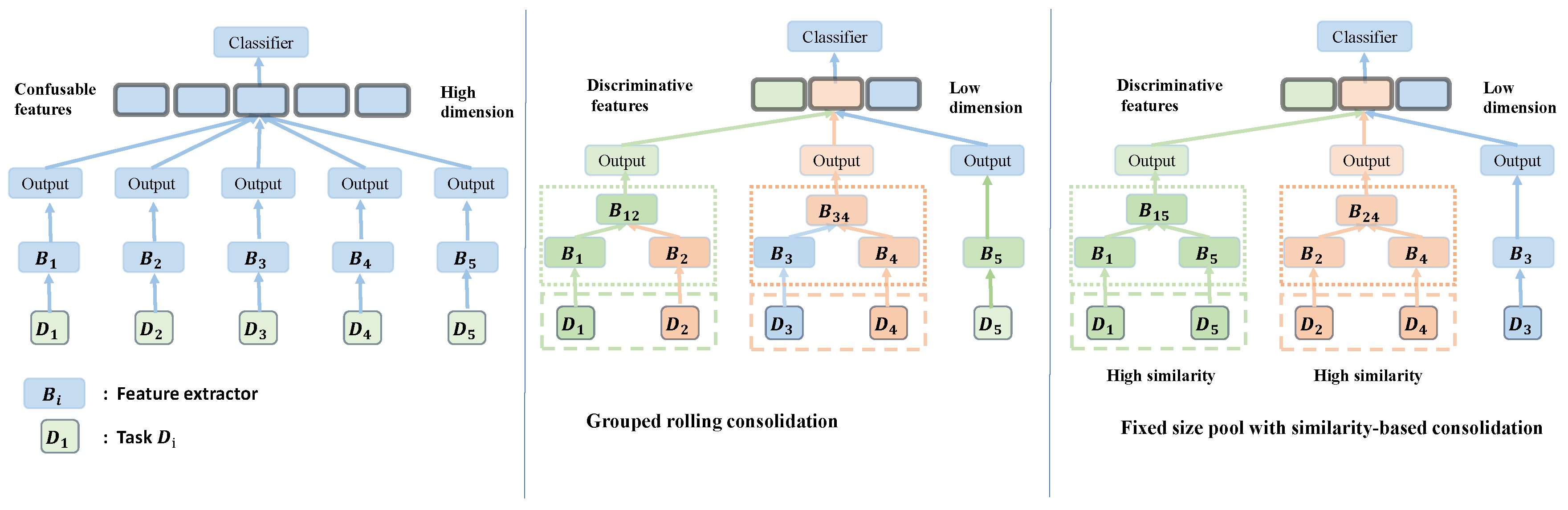
Figure 2.
Overview of Fixed-size pool with similarity-based consolidation.
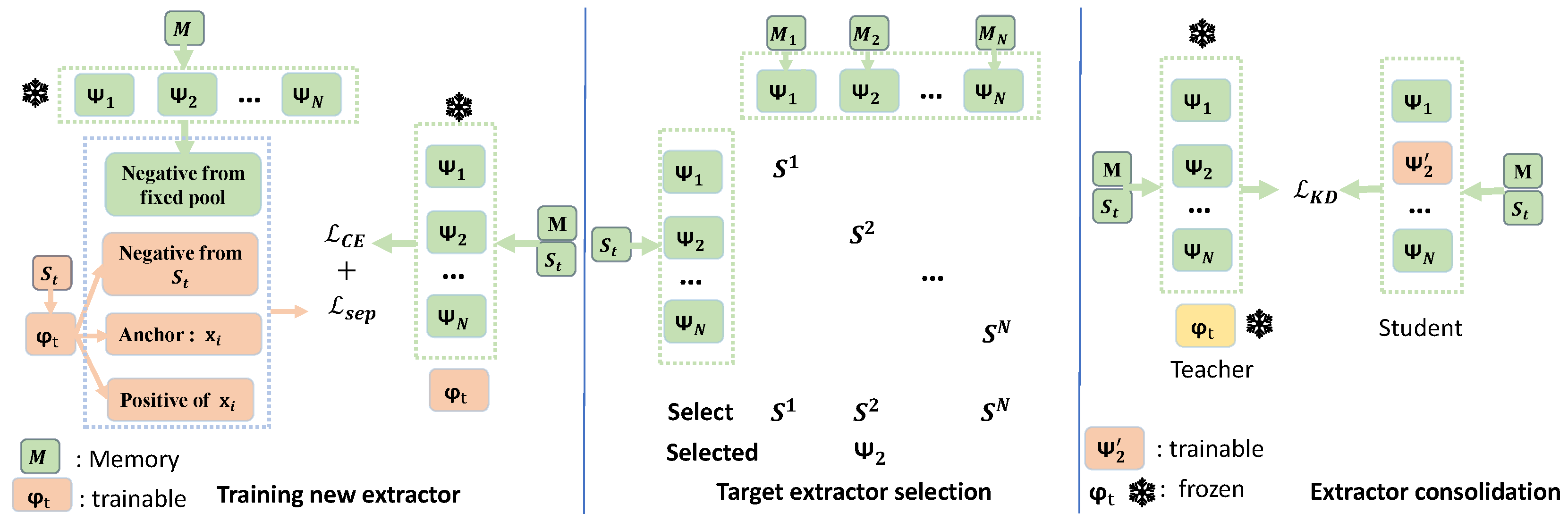
Figure 3.
Accuracy on CIFAR-100 B0S10 with different numbers of extractors. We compare our methods, fixN and grcN, with the DER baseline. Left: last-step accuracy. Right: average accuracy.
Figure 3.
Accuracy on CIFAR-100 B0S10 with different numbers of extractors. We compare our methods, fixN and grcN, with the DER baseline. Left: last-step accuracy. Right: average accuracy.
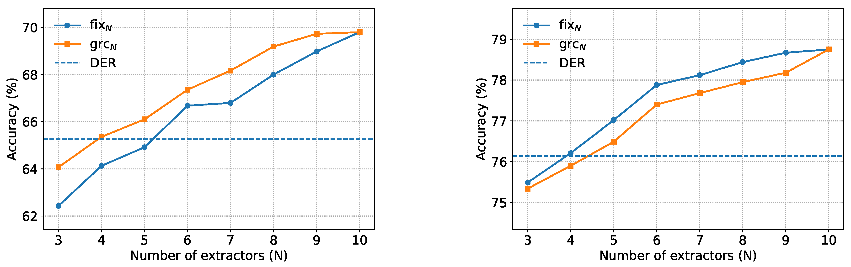
Figure 4.
Accuracy of each step on CIFAR100B0S10. We compare our methods, fixN and grcN, with the DER baseline.
Figure 4.
Accuracy of each step on CIFAR100B0S10. We compare our methods, fixN and grcN, with the DER baseline.
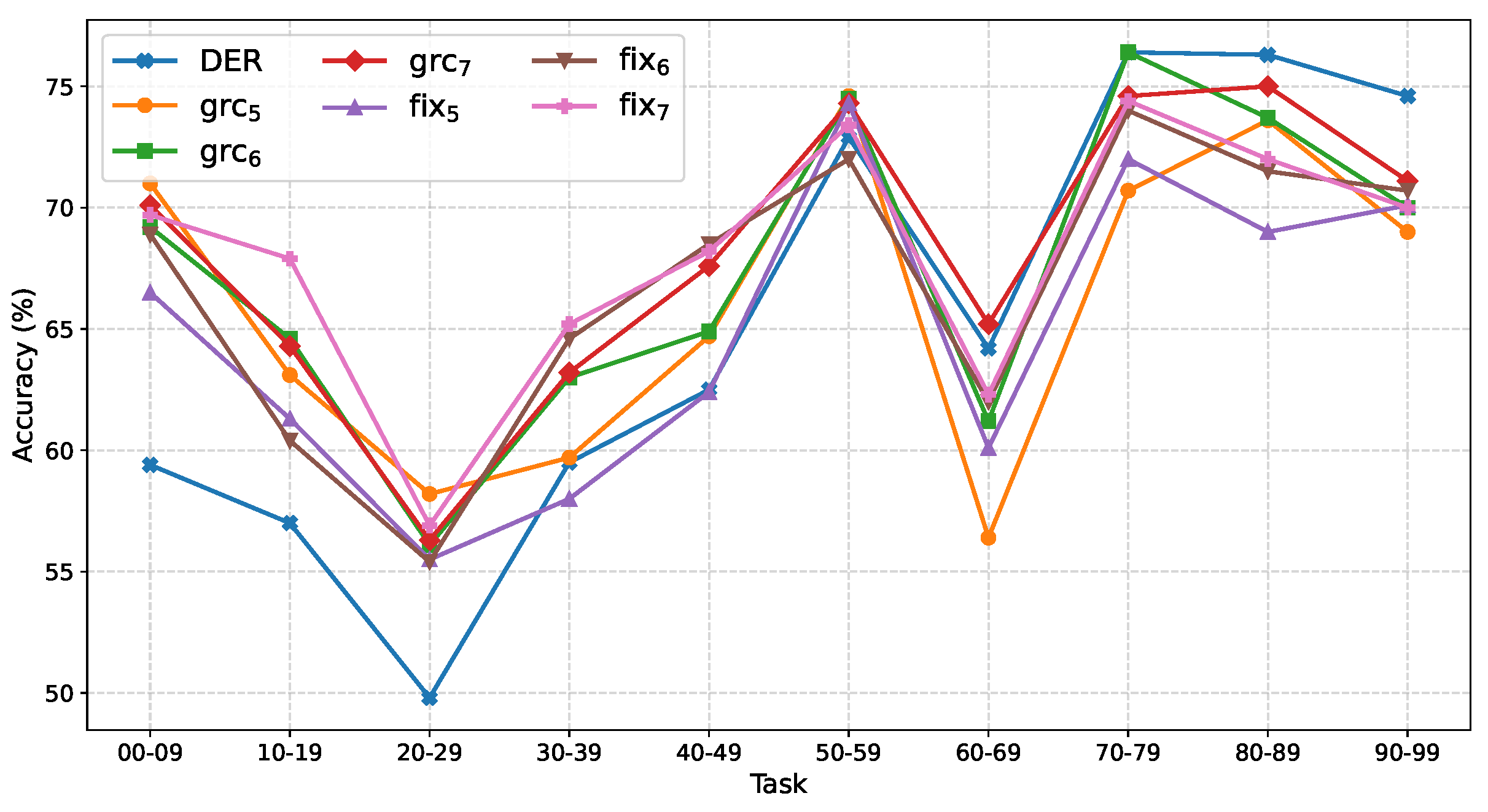
Figure 5.
Accuracy on CIFAR-100 B0S5 with different numbers of extractors. We compare our methods, fixN and grcN, with the DER baseline. Left: last-step accuracy. Right: average accuracy.
Figure 5.
Accuracy on CIFAR-100 B0S5 with different numbers of extractors. We compare our methods, fixN and grcN, with the DER baseline. Left: last-step accuracy. Right: average accuracy.
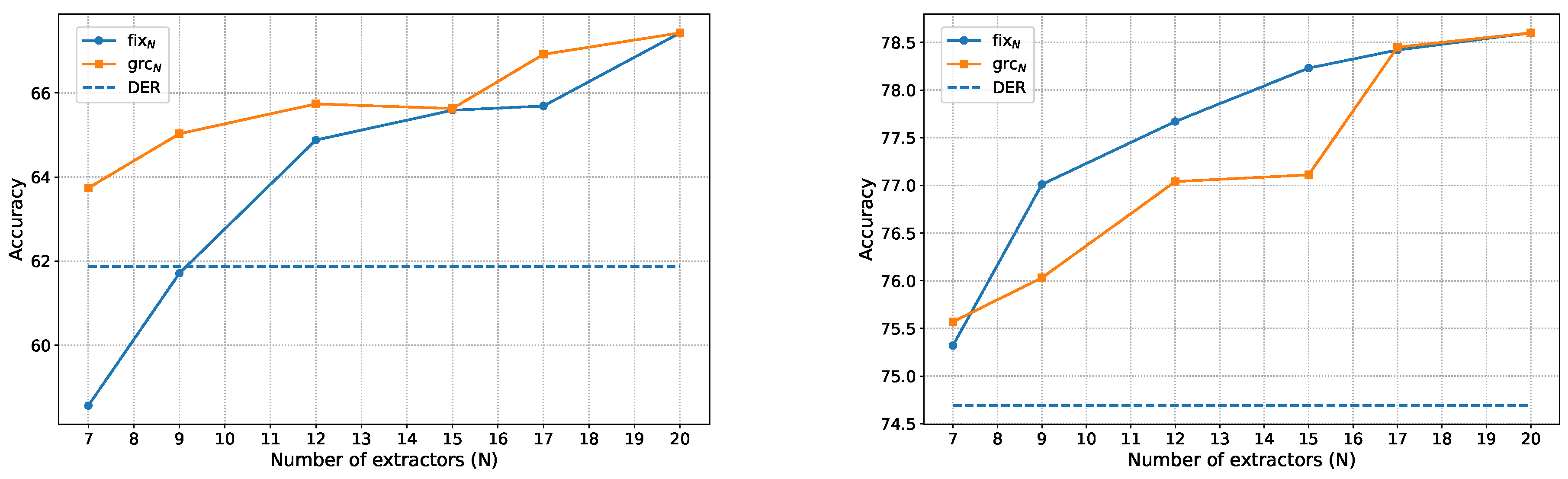
Figure 6.
t-SNE visualization on CIFAR-100. We randomly select 12 classes for visualization. Left: DER. Right: .
Figure 6.
t-SNE visualization on CIFAR-100. We randomly select 12 classes for visualization. Left: DER. Right: .
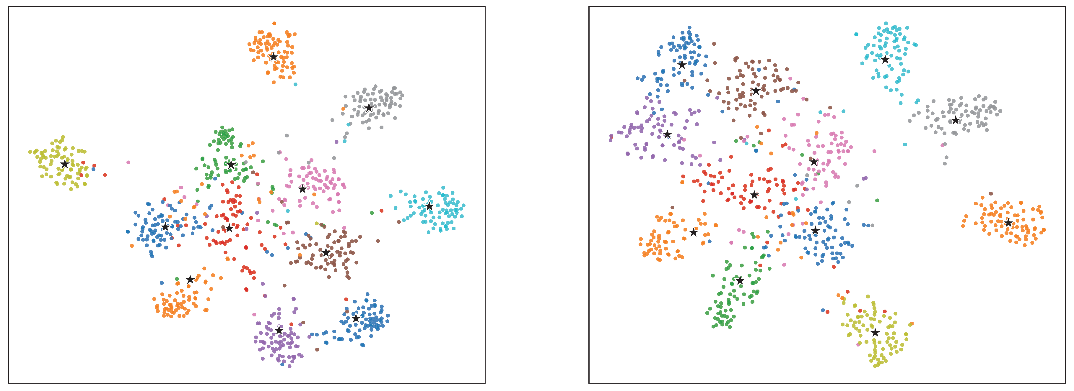
Figure 7.
Accuracy on CIFAR-100 B50S5 with different numbers of extractors. We compare our methods, fixN and grcN, with the DER baseline. Left: last-step accuracy. Right: average accuracy.
Figure 7.
Accuracy on CIFAR-100 B50S5 with different numbers of extractors. We compare our methods, fixN and grcN, with the DER baseline. Left: last-step accuracy. Right: average accuracy.
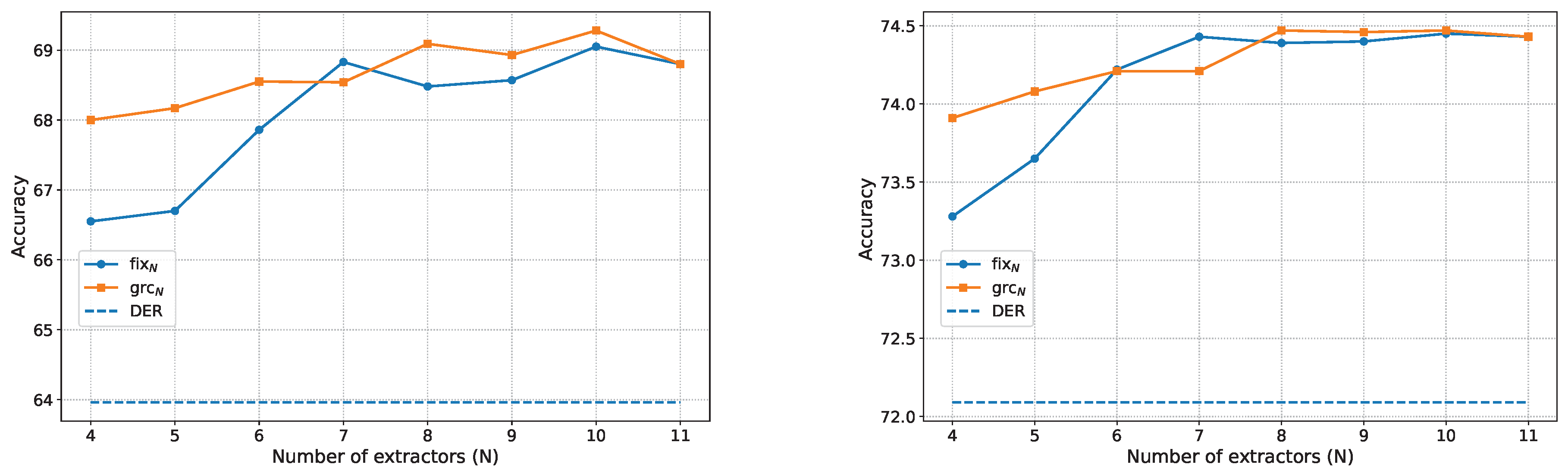
Figure 8.
Accuracy on CIFAR-100 B50S2 with different numbers of extractors for . Left: last-step accuracy. Right: average accuracy.
Figure 8.
Accuracy on CIFAR-100 B50S2 with different numbers of extractors for . Left: last-step accuracy. Right: average accuracy.
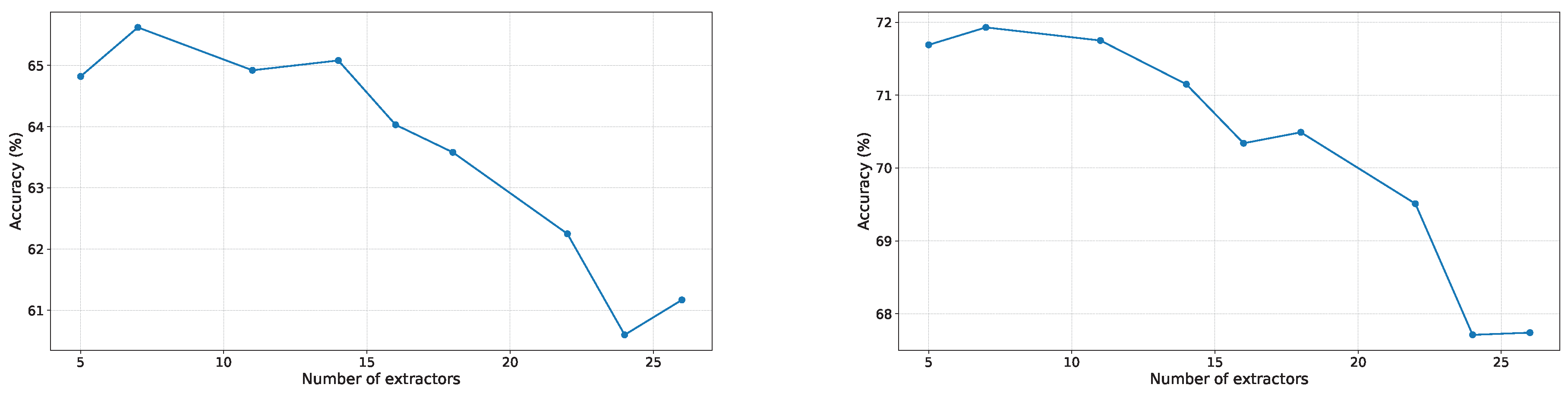
Table 1.
Last step accuracy of DER on CIFAR-100. Each task is assigned one extractor, so the number of tasks equals the number of extractors. Accuracy is reported after learning all 100 classes.
Table 1.
Last step accuracy of DER on CIFAR-100. Each task is assigned one extractor, so the number of tasks equals the number of extractors. Accuracy is reported after learning all 100 classes.
| Setting | Tasks Number | Classes per Task | Last Acc. (%) |
|---|---|---|---|
| B0S10 | 10 | 10 | 65.26 |
| B0S5 | 20 | 5 | 61.87 |
Table 2.
Results on ImageNet-100 B0S10. Results of the comparison methods are reported from [23,24,28]. The results of DyTox are based on the official corrected version.
| ImageNet-100 B0S10 | ||||
|---|---|---|---|---|
| Method | Top-1 | Top-5 | ||
| Avg | Last | Avg | Last | |
| iCaRl [2] | - | - | 83.60 | 63.80 |
| RPSNet [38] | - | - | 87.90 | 74.00 |
| BiC [15] | - | - | 90.60 | 84.40 |
| WA [16] | - | - | 91.00 | 84.10 |
| SEED [28] | - | - | - | |
| DyTox [24] | 71.85 | 57.94 | 90.72 | 83.52 |
| FOSTER [26] | 78.40 | 69.91 | - | - |
| BEEF [39] | 77.62 | 68.78 | 93.66 | 89.32 |
| DER [23] | 77.18 | 66.70 | 93.23 | 87.52 |
| 79.93 | 70.54 | 95.08 | 91.64 | |
| 79.90 | 69.78 | 94.92 | 91.44 | |
| 80.59 | 72.36 | 95.20 | 92.04 | |
| 81.01 | 71.38 | 95.36 | 91.84 | |
Table 3.
Results of the comparison methods are reported from [23,24,28]. The results of DyTox are based on the official corrected version.
| ImageNet-100 B50S5 | ||||
|---|---|---|---|---|
| Method | Top-1 | Top-5 | ||
| Avg | Last | Avg | Last | |
| UCIR [10] | 68.09 | 57.30 | - | - |
| PODNet [9] | 74.33 | - | - | - |
| TPCIL [40] | 74.81 | 66.91 | - | - |
| SEED [28] | - | - | - | |
| FOSTER [26] | 77.54 | - | - | - |
| DER [23] | 78.20 | 74.92 | 94.20 | 91.30 |
| 79.15 | 73.82 | 95.13 | 93.04 | |
| 79.08 | 74.14 | 95.30 | 93.12 | |
Table 4.
Results on CIFAR100-B0S10. Results of the comparison methods come from DyTox [24] and DER [23]. Average accuracy is recorded as Avg (%). Last step accuracy is recorded as Last (%).
| Method | Avg | Last |
|---|---|---|
| iCaRl[2] | 50.74 | |
| UCIR [10] | 43.39 | |
| BiC [15] | 53.54 | |
| WA [16] | 53.78 | |
| PODNet [9] | 41.05 | |
| RPSNet [38] | 68.60 | 57.05 |
| DyTox [24] | ||
| FOSTER [26] | 72.90 | - |
| BEEF [39] | 71.94 | 60.98 |
| BEEF-Compress [39] | 72.93 | 61.45 |
| DER [23] | 76.14 | 65.26 |
| 77.40 | 67.36 | |
| 77.88 | 66.68 |
Table 5.
Results on CIFAR100B0S5. Results of the comparison methods come from DyTox [24] and DER [23]. Average accuracy is recorded as Avg (%). Last step accuracy is recorded as Last (%).
| Method | Avg | Last |
|---|---|---|
| iCaRl [2] | 43.75 | |
| UCIR [10] | 40.63 | |
| BiC [15] | 47.02 | |
| WA [16] | 47.31 | |
| PODNet [9] | 35.02 | |
| RPSNet [38] | - | - |
| DyTox [24] | ||
| FOSTER [26] | 70.65 | - |
| BEEF [39] | 69.84 | 56.71 |
| BEEF-Compress [39] | 71.69 | 57.06 |
| DER [23] | 74.69 | 61.87 |
| 75.57 | 63.74 | |
| 77.20 | 63.22 |
Table 6.
Accuracy on CIFAR-100B50S5. Average accuracy is recorded as Avg (%). Last-step accuracy is recorded as Last (%).
Table 6.
Accuracy on CIFAR-100B50S5. Average accuracy is recorded as Avg (%). Last-step accuracy is recorded as Last (%).
| Method | Avg | Last |
|---|---|---|
| iCaRL [2] | 53.78 | - |
| BiC [15] | 53.21 | - |
| WA [16] | 57.57 | - |
| COIL[41] | 59.96 | - |
| PODNet [9] | 63.19 | - |
| Foster [26] | 69.20 | 60.42 |
| DER [23] | 72.09 | 63.96 |
| 73.91 | 68.00 | |
| 73.28 | 66.55 | |
| 74.21 | 68.55 | |
| 74.22 | 67.86 |
Table 7.
Average incremental accuracy on CIFAR-100B50S2. Average accuracy is recorded as Avg (%). Last-step accuracy is recorded as Last (%).
Table 7.
Average incremental accuracy on CIFAR-100B50S2. Average accuracy is recorded as Avg (%). Last-step accuracy is recorded as Last (%).
| Method | Avg | Last |
|---|---|---|
| iCaRL [2] | 50.60 | - |
| BiC [15] | 48.96 | - |
| WA [16] | 54.10 | - |
| PODNet [9] | 60.72 | - |
| Foster [26] | 65.99 | 56.58 |
| DER [23] | 71.45 | 63.81 |
| 71.90 | 65.36 | |
| 71.75 | 64.21 |
Table 8.
Ablation study on . Average accuracy is denoted as Avg (%), and last-step accuracy as Last (%).
Table 8.
Ablation study on . Average accuracy is denoted as Avg (%), and last-step accuracy as Last (%).
| Method | Avg (%) | Last (%) |
|---|---|---|
| DER | 76.14 | 65.26 |
| (w/o ) | 75.53 | 64.07 |
| (w/ ) | 77.40 | 67.36 |
| (w/o ) | 74.25 | 61.56 |
| (w/ ) | 77.88 | 66.68 |
Table 9.
Backward Transfer (BWT, %) comparison on CIFAR-100B0S10.
| Method | BWT |
|---|---|
| DER | -10.76 |
| GRC5 | -10.36 |
| Fix5 | -10.44 |
| GRC8 | -9.19 |
| Fix8 | -8.93 |
Disclaimer/Publisher’s Note: The statements, opinions and data contained in all publications are solely those of the individual author(s) and contributor(s) and not of MDPI and/or the editor(s). MDPI and/or the editor(s) disclaim responsibility for any injury to people or property resulting from any ideas, methods, instructions or products referred to in the content. |
© 2025 by the authors. Licensee MDPI, Basel, Switzerland. This article is an open access article distributed under the terms and conditions of the Creative Commons Attribution (CC BY) license (http://creativecommons.org/licenses/by/4.0/).
Copyright: This open access article is published under a Creative Commons CC BY 4.0 license, which permit the free download, distribution, and reuse, provided that the author and preprint are cited in any reuse.


