Submitted:
07 September 2025
Posted:
08 September 2025
You are already at the latest version
Abstract
Condition monitoring and fault diagnosis of electrical equipment are essential for ensuring the reliability and safety of modern energy and industrial systems. This paper proposes an artificial intelligence-based method for equipment fault diagnosis by integrating Quantum-Inspired Dynamic Variational Mode Decomposition (QD-VMD) with a lightweight convolutional neural network (L-CNN). QD-VMD adaptively determines the number of modes (K) and the penalty factor (α) through a quantum-state probability model with phase-guided updates, thereby enabling stable decomposition of nonstationary signals under noisy conditions. Statistical features derived from the decomposed modes in both time and frequency domains are combined into multi-scale feature tensors, which are then classified by an L-CNN employing depthwise separable convolutions and channel attention. The proposed method achieves 99.95% accuracy on the CWRU bearing dataset with approximately 55,000 parameters and 1.04 × 10⁻³ GFLOPs, while maintaining an average inference latency of about 2.5 ms on embedded hardware, supporting real-time edge deployment. Cross-domain evaluations on datasets from power systems and new energy vehicles yield precision, recall, and F1-scores all greater than or equal to 0.987, demonstrating strong robustness across heterogeneous operating conditions. Reconstruction experiments further show that QD-VMD preserves critical fault-related structures with a low global mean squared error (MSE). These results confirm that combining robust signal decomposition with compact learning architectures provides an effective AI-based solution for fault diagnosis of electrical equipment, with potential applicability to insulation monitoring and related reliability tasks.
Keywords:
Variational Mode Decomposition
; Quantum-Inspired Algorithm
; Lightweight Convolutional Neural Network
; Fault Diagnosis
; Edge Intelligence
1. Introduction
Fault signal extraction, analysis, and diagnosis in industrial equipment are critical for ensuring production safety and improving operational efficiency. These challenges are pervasive across a broad spectrum of domains, including rotating machinery, power systems, and new energy equipment. For example, vibration signals from rolling bearings in rotating machinery, transient electrical signals in power transmission lines, and multiphysics coupling signals in the drivetrains of new energy vehicles all share common characteristics such as non-stationarity, strong noise interference, and feature ambiguity. These shared traits pose significant challenges to the accurate identification of early-stage faults across various sectors, including rotating machinery, power systems, and electric vehicles [1]. Timely and effective fault diagnosis not only mitigates economic losses caused by unexpected downtime but also helps prevent catastrophic safety incidents, thereby playing a vital role in intelligent manufacturing and predictive maintenance paradigms [2].
The primary bottleneck in fault diagnosis arises from the inherent complexity of vibration signals. On one hand, these signals are typically nonlinear and non-stationary, often influenced by diverse and mixed sources of noise present in real-world industrial environments. As noted by Mohd Ghazali and Rahiman [3], dynamic variations in operational speed, load, and fault conditions are key contributors to signal non-stationarity, posing substantial challenges to conventional signal processing techniques. Furthermore, noise often masks critical fault-related frequencies, complicating the extraction of discriminative features. For instance, impact characteristics of bearing vibration signals may be buried in broadband noise; high-frequency decay components in power system fault transients can be easily mixed with harmonic interference; and vibration-electrical coupled signals in new energy drivetrains may involve complex multiphysical-field disturbances [4]. On the other hand, although fault signals from different domains share certain statistical and structural properties, their specific manifestations can differ significantly. Mechanical systems are primarily characterized by the distribution of vibration energy, power systems depend on transient variations in voltage and current, and new energy vehicles require integration of multidimensional information such as motor speed, torque, and vibration. This heterogeneity places stringent demands on the generalization capability of fault diagnosis methods across different application domains [5].
Despite significant advancements, current fault diagnosis techniques still exhibit notable limitations when addressing the aforementioned challenges. At the signal processing level, traditional methods such as the Fast Fourier Transform (FFT) identify fault characteristic frequencies by transforming time-domain sequences into frequency-domain representations [6]. However, because FFT assumes signal stationarity, it fails to effectively capture the time-varying features of non-stationary signals, often leading to inaccurate feature extraction. The Short-Time Fourier Transform (STFT) improves upon this by segmenting signals and applying FFT within a sliding window to produce time-frequency representations [7]. Although STFT provides some capability for handling non-stationary signals, its effectiveness is constrained by the fixed window size, resulting in a trade-off between time and frequency resolution that limits its performance under dynamic conditions.
Wavelet Transform (WT), which employs scalable and translatable wavelet basis functions for multiresolution analysis [8], partially overcomes the limitations of STFT by providing better localization of transient events in the time-frequency domain. However, its effectiveness heavily depends on the proper selection of the wavelet basis; inappropriate choices may introduce significant deviations in the analysis results. Empirical Mode Decomposition (EMD), an adaptive decomposition technique [9], decomposes signals into a series of Intrinsic Mode Functions (IMFs) without requiring predefined basis functions. EMD is well-suited for nonlinear and non-stationary signals, enabling extraction of features across multiple frequency scales. Nevertheless, it suffers from mode mixing and endpoint effects, which can degrade the accuracy of the decomposition.
To address these issues, techniques such as Ensemble Empirical Mode Decomposition (EEMD) and Complementary Ensemble Empirical Mode Decomposition with Adaptive Noise (CEEMDAN) have been developed, introducing white noise to suppress mode mixing [10,11]. However, these approaches may still leave residual noise, limiting their effectiveness in real-world applications. Variational Mode Decomposition (VMD), an emerging signal decomposition technique, addresses many of the drawbacks of EMD by decomposing a signal into a set of band-limited intrinsic mode functions. VMD formulates the decomposition as a constrained variational optimization problem, minimizing the sum of the bandwidths of the modes while ensuring that their sum reconstructs the original signal. Supported by solid mathematical foundations, VMD exhibits strong robustness in noisy environments, making it highly attractive for fault diagnosis tasks. For example, Dibaj et al. [12] demonstrated its effectiveness in isolating fault features in rotating machinery.
However, the performance of VMD is highly sensitive to its key parameters, specifically the number of modes (K) and the penalty factor (α). Improper selection can result in over-decomposition or under-decomposition, negatively impacting the quality of extracted features. Traditional parameter selection typically relies on empirical knowledge or extensive trial-and-error, which lacks systematic guidance and can be computationally inefficient.
At the model level, deep learning techniques--particularly Convolutional Neural Networks (CNNs)--have made significant advances in fault diagnosis due to their ability to automatically learn hierarchical features from raw or preprocessed vibration signals, thereby reducing reliance on manual feature engineering and domain expertise. For example, Azamfar et al. [13] highlighted the superior capability of CNNs in capturing complex signal patterns. Researchers have developed various CNN architectures tailored to vibration signal characteristics, such as transforming time-domain signals into two-dimensional time–frequency images for classification via 2D CNNs [14], or employing 1D CNNs to directly process time-series data [15].
However, conventional CNNs typically require large amounts of labeled data for training and are computationally intensive, with model sizes often exceeding 10⁶ parameters. This high computational demand limits their suitability for deployment on resource-constrained edge devices. With the advancement of Industry 4.0, edge computing has become increasingly important in industrial applications. By processing data locally near the source, edge computing significantly reduces network latency and enhances real-time responsiveness, enabling localized monitoring and rapid fault diagnosis. It also decreases dependence on cloud infrastructure, lowers bandwidth requirements, and improves data privacy.
Nevertheless, edge devices are inherently limited in computational power, memory, and energy capacity. Deep CNNs with large parameter counts and deep architectures are challenging to deploy in such environments, as their high computational cost and memory usage hinder real-time inference. Additionally, deep learning models are sensitive to data quality--noise can bias feature learning--and they generally lack interpretability, which is a critical concern in industrial applications that demand transparent decision-making.
To address these challenges, lightweight CNN architectures such as MobileNet and EfficientNet have been proposed [16]. These models reduce parameter count and computational load through techniques like depthwise separable convolutions and global average pooling, and further improve efficiency via model quantization and hardware acceleration. While these methods enhance suitability for edge deployment, achieving a balance between diagnostic accuracy and computational efficiency remains a challenge for fault diagnosis tasks.
To overcome the threefold challenge of (1) non-stationary and noisy vibration signals, (2) computational inefficiency of deep models on edge platforms, and (3) limited model generalization, this study proposes a bearing fault diagnosis method that integrates Quantum-Inspired Optimization for Variational Mode Decomposition (QD-VMD) with a Lightweight Convolutional Neural Network (L-CNN). The proposed method first applies VMD to decompose vibration signals into intrinsic mode functions (IMFs). A quantum-inspired optimization algorithm is then used to adaptively optimize the critical VMD parameters, including the number of modes (K) and the penalty factor (α), ensuring high-quality decomposition even under noisy conditions. Compared with traditional optimization approaches, quantum-inspired methods explore the parameter space more efficiently and are less susceptible to local optima.
Next, a feature matrix is constructed from the decomposed IMFs, containing both time-domain features (e.g., kurtosis and skewness) and frequency-domain features (e.g., spectral amplitude and peak frequency). These features are input to a lightweight CNN designed with depthwise separable convolutions, global average pooling, channel attention mechanisms, and batch normalization, substantially reducing computational complexity while maintaining high diagnostic accuracy. Furthermore, the model is optimized using mixed-precision quantization and TensorRT acceleration, minimizing inference latency and enabling efficient deployment on resource-constrained edge devices.
To validate the effectiveness and generalizability of the proposed method, a multi-level experimental framework is employed. Core experiments are conducted on the Case Western Reserve University (CWRU) bearing dataset, serving as the primary benchmark. Through analysis of parameter optimization trajectories, quantitative evaluation of decomposition performance, and assessment of classification accuracy, the QD-VMD–L-CNN method is validated in terms of diagnostic accuracy, computational efficiency, and model compactness. Results are compared against baseline models such as conventional CNNs to demonstrate relative performance gains.
In addition, generalization experiments are performed using the IEEE PES Transmission Line Fault Dataset (IEEE PES Dataset) and the New Energy Vehicles Transmission System Dataset (NEV Dataset). These experiments involve cross-domain transfer testing to evaluate the method’s adaptability to heterogeneous signal types. Metrics such as Precision, Recall, and F1-score are quantitatively analyzed, and real-time inference performance on edge devices is assessed to confirm the model’s cross-domain generalization capability. By combining both domain-specific validation and cross-scenario testing, this experimental setup provides a comprehensive verification of the practical applicability of the QDVMD–L-CNN framework in complex industrial environments.
The main contributions of this study are as follows:
(1) Systematic Construction of the QDVMD-LCNN Framework:
A novel fault diagnosis algorithm is proposed that integrates Quantum-Inspired Optimization, Variational Mode Decomposition (VMD), and a Lightweight Convolutional Neural Network (L-CNN) into a unified framework, termed QDVMD-LCNN. This approach bridges the gap between signal processing and classification in traditional methods, enhancing feature extraction robustness under strong noise and improving deployment efficiency on edge devices through the cross-domain fusion of quantum-inspired mechanisms and deep learning.
(2) Quantum-Inspired Optimization for VMD (QD-VMD):
A quantum-inspired optimization strategy is developed to adaptively determine the key VMD parameters--the number of modes (K) and the penalty factor (α)--which significantly improves decomposition quality and robustness under noisy conditions.
(3) Lightweight Convolutional Neural Network Architecture:
A low-complexity L-CNN architecture is designed using depthwise separable convolutions, global average pooling, and model quantization, enabling high-accuracy fault diagnosis with substantially reduced computational complexity and memory usage, making it well-suited for real-time inference on resource-constrained edge devices.
(4) Validation of Effectiveness and Generalizability Across Multiple Scenarios:Experiments on the CWRU bearing dataset demonstrate high classification accuracy, extremely low false positive rates, and minimal inference latency, fully meeting the demands of real-time industrial diagnostics. Furthermore, cross-domain evaluations with diverse datasets validate the model’s generalization capability across heterogeneous data and multi-physical domains, laying a foundation for the development of unified and scalable health monitoring platforms.
The aforementioned contributions systematically address three common challenges: (1) the difficulty of feature extraction caused by signal non-stationarity and strong noise interference; (2) the high computational resource demands of deep learning models, which hinder deployment on edge devices; and (3) limited cross-domain generalization capability. This work establishes a comprehensive technical pipeline of “adaptive parameter optimization--lightweight modeling--cross-domain validation,” which simultaneously enhances the robustness of signal decomposition via a quantum-inspired mechanism, overcomes resource constraints for edge deployment through a lightweight architecture, and verifies the method’s universal applicability through multi-domain validation. Together, these advances represent a systematic breakthrough that overcomes key bottlenecks in existing technologies.
The main chapters of this work are organized as follows:
Chapter 1 reviews related work, elucidates the mathematical principles of VMD and its applications across multiple domains, and discusses the core mechanisms of Convolutional Neural Networks (CNNs) along with recent advances in lightweight model design, thus laying the theoretical foundation for the proposed method.
Chapter 2 details the technical aspects of the proposed diagnostic algorithm, including quantum-inspired VMD parameter optimization based on quantum sampling and rotation gate mechanisms, as well as the architecture design, regularization strategies, and deployment optimizations of the lightweight CNN.
Chapter 3 presents core experiments on the CWRU bearing dataset, analyzing parameter optimization trajectories, evaluating signal decomposition quality, and validating classification performance to demonstrate effectiveness within a single domain.
Chapter 4 conducts cross-domain generalization tests on datasets from power system transient signals and new energy vehicle transmission systems, verifying the method’s adaptability to heterogeneous scenarios.
Chapter 5 discusses the advantages, limitations, and future research directions of the method, analyzes practical application challenges, and proposes potential improvements.
Chapter 6 concludes the work by summarizing the core contributions and highlighting the algorithm’s efficacy and its support for multi-domain equipment health monitoring.
2. Related Work
2.1. VMD
VMD is an adaptive signal decomposition method designed to decompose non-stationary signals into a set of band-limited IMFs, with each IMF representing characteristic components at specific frequency scales. The core idea of VMD lies in formulating and solving a variational optimization problem, which aims to minimize the sum of the bandwidths of all modes while ensuring that the reconstructed signal remains consistent with the original input. The mathematical formulation is expressed as follows:
Here, denotes the -th IMF, represents its corresponding center frequency,and is the original input signal. refers to the Dirac delta function,while denotes the convolution operator.VMD solves the variational problem via an iterative scheme based on the Alternating Direction Method of Multipliers (ADMM), enabling effective separation of modes.
Compared with EMD, VMD offers stronger mathematical rigor and superior resistance to mode mixing, particularly exhibiting higher robustness in noisy environments. It does not require predefined basis functions, making it well-suited for the decomposition of nonlinear and non-stationary signals. As a result, VMD has been widely applied in the analysis of vibration signals in scenarios such as rotating machinery and gearboxes.
2.2. CNN
CNN are a class of deep learning models that have been widely applied in fields such as image recognition and speech processing. The core architecture of CNN typically consists of convolutional layers, pooling layers, and fully connected layers. The convolutional layer extracts local features from the input data using a sliding window mechanism, which can be mathematically expressed as:
Here, represents the input signal, is the convolution kernel (filter), denotes the convolution output (feature map), refers to the kernel size.This operation is particularly well-suited for capturing temporal features in vibration signal time series. The pooling layer reduces the dimensionality of feature maps to lower computational cost, while the fully connected layer is used for classification or regression tasks.In the context of mechanical fault diagnosis, CNN are capable of automatically extracting high-level features from raw vibration signals or their time-frequency representations--such as spectrograms generated via Short-Time Fourier Transform (STFT) or wavelet transform--thus significantly reducing reliance on hand-crafted feature engineering.
Compared with traditional fault diagnosis methods, CNN can automatically extract high-level semantic features from raw vibration signals or their time-frequency representations (e.g., spectrograms generated via STFT or wavelet transform), thereby reducing the reliance on manual feature engineering. CNN-based approaches have achieved high classification performance on publicly available mechanical fault datasets. The convolutional mechanism, characterized by local receptive fields and parameter sharing, offers translation invariance and enables efficient feature compression.
3. Methodology
Building upon the aforementioned works, this paper proposes a fault diagnosis algorithm that integrates Quantum-Inspired Parameter Optimization (QIPO), Variational Mode Decomposition (VMD), and a Lightweight Convolutional Neural Network (L-CNN). The overall framework is illustrated in Figure 1.
The diagram illustrates the end-to-end process from parameter optimization to fault classification. The algorithm is divided into three phases:
Phase I: A parameter optimization module based on quantum bit mechanics (QIPO) adaptively searches for the optimal configuration of key VMD parameters--specifically, the number of modes (K) and the penalty factor (α).
Phase II: The optimized parameters are then input into the VMD module to perform multi-modal decomposition of non-stationary signals and construct multi-scale feature representations.
Phase III: A lightweight convolutional neural network (L-CNN) is employed to classify the resulting feature tensor and identify fault categories.
This method establishes a closed-loop structure encompassing parameter search, signal decomposition, and model decision-making. It is characterized by high adaptability, strong scalability, and compatibility with embedded deployment, making it well-suited for complex signal recognition tasks in industrial environments.3.1. Subsection
3.1. Phase I: QIPO Process
To address the limitations of Variational Mode Decomposition (VMD)--particularly its reliance on manually defined parameters and its limited adaptability to complex operating conditions--this phase introduces a Quantum-Inspired Parameter Optimization (QIPO) mechanism based on quantum probability modeling. The QIPO framework comprises three key steps: quantum state probability modeling, probability updating driven by reward feedback, and phase-guided local convergence via quantum rotation gates.
Step 1: Quantum State Probability Modeling
In this study, the parameter space is encoded as a finite-dimensional discrete set of quantum states, and a probability vector of length is constructed, where is the number of qubits, corresponding to available states. Each quantum state is uniquely mapped to a combination of VMD parameters (, ).
At the initial stage, the quantum state vector is modeled using a uniform distribution:
Here, denotes the probability of the -th quantum state, and i is the state index ranging from 0 to . This strategy is conceptually analogous to the Hadamard transform in quantum computing, which produces an unbiased superposition across the entire parameter space, serving as a basis for global exploration. The initialization scheme, inspired by the Hadamard Transform [17], can be regarded as generating a uniform coverage of the parameter space, providing a broad foundation for subsequent optimization.
To implement the mapping between quantum states with uniform distribution as defined in Equation (3) and VMD parameters, a discretized parameter space is constructed physically on the upper level. Since continuous hyperparameters are difficult to directly associate with discrete quantum states in a one-to-one manner, this study discretizes the number of modes K and the penalty factor α into the intervals and , respectively, and divides them into and segments. This forms a two-dimensional search grid of size . Each grid cell is uniquely mapped to a quantum state , ensuring a one-to-one correspondence between the discretized parameter space and the quantum state space of size. This mapping provides physical support for the quantum initialization defined in Equation (3), and underpins the reward-driven probability update mechanism introduced in Step 2.
This step establishes a one-to-one correspondence between the quantum states and the VMD core parameters (number of modes K and penalty factor α) through uniform probability initialization and mapping. It lays the foundation for efficient search and optimal determination of VMD parameters in the subsequent machine-driven optimization process.
Step 2: Probability Update Driven by Reward Feedback
To evaluate the quality of each parameter combination, a VMD decomposition metric based on an energy criterion is introduced:
Here, denotes the sum of the bandwidth energy across all modes, is the -th mode component, and is the number of modes. A smaller indicates better mode compactness and decomposition performance.
To balance decomposition quality and model complexity, the following reward function is constructed:
where is the reward score, is a small positive constant (typically 0.0001), and
is the penalty factor. ,,are the weights for the three components of the evaluation metric. This reward function penalizes energy and model complexity to prevent overfitting.
After obtaining the reward score for each quantum state, the probability vector is updated using a sampling mechanism that favors states with higher rewards. To this end, a normalized softmax-like function is adopted to adjust the state probabilities as follows:
Here, is the updated probability of the -th state, reflecting its optimization result. is the previous probability before updating. The scaling factor controls the strength of selection. If the distribution becomes overly concentrated, a sampling mechanism based on probability truncation is used to suppress overfitting and maintain exploratory diversity across the search space.
In this step, the decomposition index (Equation 4) is used to quantify VMD performance. Combined with the reward score (Equation 5), the parameter pair (K,α) is comprehensively evaluated. Through probability updates based on Equation (6), superior parameter combinations are sampled with higher probability, enabling adaptive search convergence and enhanced parameter clustering.
Step 3: Phase-Guided Local Convergence via Quantum Rotation Gates
In the post-exploration phase, a Quantum Rotator mechanism is introduced to simulate phase rotation, thereby refining the search direction and convergence efficiency. In this mechanism, a phase direction vector is defined for each quantum state, where the state amplitude is represented as a complex number . The phase controls the interference direction in the search space. The quantum rotation operation updates the amplitude according to:
Here, is the updated amplitude of the -th quantum state, reflecting the optimization effect. is the amplitude before updating. The rotation angle is determined by the reward score and the learning rate . To implement the strategy of “coarse exploration first, fine exploitation later,” a staged decay strategy is adopted for :
Here, is the time-dependent learning rate,
denotes the turning point from global to local search, and is the decay coefficient. This mechanism enables broad search in the early stage, while gradually narrowing the search scope and enhancing exploitation ability as rewards accumulate.
Under the action of the quantum rotation gate, the amplitude and phase of each state’s solution probability are recalculated. After that, normalization is applied using the following update rule:
This update process effectively simulates the constructive and destructive interference mechanisms observed in quantum systems: states with higher reward values experience larger phase shifts, leading to constructive interference in the superposition state and significantly increasing their sampling probabilities; in contrast, states with lower rewards are gradually suppressed due to destructive interference. This results in adaptive guidance of the search direction, thereby enhancing the sampler’s local convergence capability and its ability to escape local optima in complex non-convex spaces.
In this step, quantum rotation gates (Equations 7–8) are used to adjust the phase of each quantum state. Constructive interference is employed to strengthen the sampling probability of high-reward VMD parameter pairs (K,α) (as formulated in Equation 9), enabling fine-grained optimization and stable convergence of the parameter search process, ultimately leading to the determination of the optimal VMD parameter configuration.
3.2. Phase II: VMD Process
In this phase, the VMD parameter configuration obtained from Phase I is used to decompose the original signal into intrinsic mode components and to construct a corresponding feature tensor. This structured output is designed to serve as input for downstream neural network models. The process is divided into two steps:mode decomposition and feature construction, and signal reconstruction with fidelity constraints.
Step1: Mode Decomposition and Feature Tensor Construction
For the input signal , the VMD algorithm is employed to decompose it into Intrinsic Mode Functions (IMFs), denoted as . VMD achieves mode clustering and frequency band separation through the optimization objective in Equation (1). The decomposition is performed using an iterative Alternating Direction Method of Multipliers (ADMM), ensuring convergence to a stable spectral decomposition result.
Upon completion of the decomposition, statistical features in the frequency domain are extracted from each IMF to form a feature vector ,including metrics such as energy, entropy, mean square root,etc. All feature vectors are then sorted in descending order according to the center frequency of the corresponding modes, and stacked to construct a two-dimensional feature tensor:
Here, X serves as the final feature representation tensor for input into neural networks. It has advantages in structural regularity, information compactness, and frequency consistency, facilitating stable and efficient downstream modeling.
Step 2: Signal Reconstruction and Structural Fidelity Design
To verify whether the constructed features retain frequency separation while accurately reconstructing the original signal characteristics, a reconstruction mechanism is designed to assess fidelity. Each IMF is summed over time to reconstruct the signal, expressed as:
Here, denotes the signal reconstructed from the IMFs. The reconstruction accuracy is evaluated by comparing it with the original signal , using Mean Squared Error (MSE) as the metric to measure structural fidelity.
Here, denotes the signal length, and the MSE represents the average deviation between the reconstructed signal and the original signal. This metric reflects the effectiveness of the reconstruction process in preserving the signal’s dynamic characteristics. A lower MSE indicates greater information retention during IMF decomposition, resulting in more reliable and expressive representations. Furthermore, this structure enables verification of both the frequency stability of the modal sequence and inter-sample consistency, thereby providing a semantically interpretable and controllable input foundation for subsequent convolutional modeling.
3.3. Phase III: L-CNN
After multi-scale modal feature extraction by QD-VMD, an efficient classifier is needed to achieve high-precision fault identification across different modalities and scenarios. Given that real-world industrial deployments often rely on resource-constrained edge devices (e.g., NVIDIA Jetson Nano), this study proposes a Lightweight Convolutional Neural Network (L-CNN) to balance diagnostic speed, energy efficiency, and classification accuracy.
3.3.1. Network Architecture Design
The overall architecture of the proposed L-CNN is illustrated in Figure 2, which outlines the modular structure and feature flow of the network. This facilitates understanding of parameter connectivity and information propagation across different stages of the model.
As shown in Figure 2, the input to the model is a modal fusion feature tensor of size (512,K,1), where 512 denotes the number of time steps, and K is the number of modes extracted by QD-VMD. The architecture is designed as follows:
(1) Layer: The input tensor is processed by a SeparableConv2D layer with a kernel size of 3×3, 32 output channels, and ‘same’ padding. This layer decouples spatial and channel-wise convolutions, significantly reducing the number of parameters and computational cost while maintaining effective feature perception.
(2) Layer: The extracted feature maps are normalized to accelerate training and improve numerical stability. This is followed by a Swish activation function, which enhances non-linear representation capabilities. Its smooth derivative characteristics help mitigate gradient vanishing in lightweight models.
(3) Layer: A depthwise convolution is applied to each channel independently, allowing for enhanced modeling of local patterns within each mode and further improving computational efficiency. The output is then reshaped into a one-dimensional sequence via a Reshape Layer to align with the subsequent temporal processing steps.
(4) Layer: A max pooling operation with a pool size of 2 is used to downsample the sequence, retaining salient features and reducing redundancy and model complexity. To further improve responsiveness to key features, a lightweight Channel Attention Mechanism is introduced, dynamically enhancing fault-relevant information by learning the importance weights of each channel.
(5) Layer: In the aggregation stage, global average pooling is applied across all channels, replacing fully connected layers to compress features, reduce parameter redundancy, and improve robustness to input variations. A Dense Layer with 128 units is then used, activated by the Swish function and regularized with an L2 penalty (coefficient: 1e-4), enhancing feature fusion while preventing overfitting. To further improve generalization under small-sample conditions, a Dropout Layer (dropout rate: 0.4) is applied to simulate input noise and increase training robustness.
(6) Output Layer: A Dense output layer with 10 units and a Softmax activation is used to produce the final classification results, mapping high-dimensional features to probabilities over ten bearing fault categories.
To support the architectural design, Table 1 lists the parameter settings and output dimensions of each layer in L-CNN, clearly indicating the model compression path and key computational stages,where K is the number of models.
3.3.2. Regularization and Model Compression
To prevent overfitting and control model size, L-CNN incorporates regularization and compression mechanisms in the fully connected layers. Specifically, L2 regularization is applied via kernel_regularizer=tf.keras.regularizers.l2(1e-4) to penalize large weights, promote network sparsity, and reduce storage overhead.
Additionally, strategic Dropout with a rate of 0.4 is introduced after the Dense layer to enhance generalization capability. Unlike some studies that apply dropout directly to convolutional layers, this design restricts dropout to the fully connected layers, effectively avoiding interference with feature extraction efficiency while significantly reducing inference computational cost.
3.3.3. Overall Architectural Optimization
The L-CNN architecture employs a hierarchical feature extraction strategy, progressing from shallow to deep layers to incrementally aggregate both local and global information. As illustrated in Figure 2, the initial layers use SeparableConv2D to extract localized receptive features, followed by DepthwiseConv2D and a channel attention mechanism to enhance feature representation. Final classification is performed using GlobalAveragePooling1D and Dense layers.
Additionally, L-CNN supports multi-branch inputs, enabling parallel processing of various feature types extracted by QD-VMD, such as time-domain features (e.g., peak value, kurtosis) and frequency-domain features (e.g., spectral magnitude, peak frequency). Select layers incorporate a weight-sharing mechanism to reuse parameters across branches, improving both training and inference efficiency. This design allows L-CNN to flexibly adapt to a wide range of fault diagnosis scenarios, including--but not limited to--bearings, gearboxes, and power equipment in industrial systems.
3.3.4. Quantization and Deployment Optimization
To meet the latency and power constraints of edge devices, L-CNN is designed to be fully compatible with INT8 quantization. All convolutional layers are coupled with Batch Normalization and Swish activation functions to maintain inference accuracy after quantization. Intermediate feature tensor dimensions are carefully reduced--for example, from (512, K, 32) to lower channel dimensions--to minimize memory access and energy consumption.
At inference, computational complexity is controlled to approximately 0.00104 GFLOPs, ensuring strict adherence to low-latency and low-power requirements for industrial edge deployment.
With this design, the final L-CNN model supports joint modeling of multi-modal vibration and electrical signal features extracted by QD-VMD. The total parameter count is approximately 5.5 × 10⁴, with a memory footprint of about 0.21 MB, demonstrating strong model compactness and adaptability. The architecture integrates depthwise separable convolutions, Batch Normalization, Swish activation, channel attention, and global pooling-based classification, achieving an effective balance between computational efficiency and expressive capability.
4. Core Experiments: Bearing Fault Diagnosis
4.1. Experimental Design
This section systematically verifies the feasibility and effectiveness of the proposed integrated model through step-by-step experiments, encompassing the entire pipeline from quantum-inspired optimization to feature extraction and fault classification. To ensure the objectivity and reproducibility of the experimental results, detailed descriptions of the experimental platform configuration and dataset construction are provided as the foundation for the subsequent procedures.
4.1.1. Experimental Setup
The experimental platform was designed to balance computational performance with deployment adaptability. During training, a high-frequency multi-threaded CPU and high-speed storage were employed to meet the data throughput and caching requirements of feature extraction and model iteration. For inference, the system targeted edge deployment, utilizing toolchains optimized for deep learning inference to ensure stable performance of the lightweight model under resource-constrained conditions.
The core model was developed using TensorFlow and Keras, with GPU acceleration provided by CUDA/cuDNN, significantly accelerating training convergence. Signal processing tasks were implemented with the SciPy and Librosa libraries for filtering and time-frequency analysis, respectively, supporting effective feature extraction from vibration signals. To meet deployment and application requirements, TensorRT was integrated for INT8 quantization, enabling latency control and memory optimization for energy-efficient, high-performance operation on edge devices.
Visualization of experimental results was conducted using Matplotlib 3.6.2 [18] and Seaborn 0.12.2 [19], two widely used Python libraries for data visualization, to support comprehensive performance comparison and algorithm evaluation.
All signal features were normalized during feature engineering and visualization to unify the units of various statistical metrics. The unit “a.u.” (arbitrary unit) denotes dimensionless normalized values, while “a.u.²” represents energy-related metrics, facilitating consistent comparison and visualization across different signal dimensions.

Table 2.
Experimental Configuration Details.
| Category | Subcategory | Specific Configuration | Main Purpose |
| Hardware | Training Platform | Intel Core i7-11800H (8 cores, 16 threads, base frequency 3.2 GHz) + 16 GB DDR4 + SSD (≥ 3500 MB/s) | Supports signal preprocessing and model training with high-performance computing resources |
| Software | Algorithm/Tool chain | Python 3.8 + TensorFlow 2.12 + Keras + CUDA 11.6 / cuDNN 8.3 | Builds lightweight models and accelerates training and inference via GPU |
| Signal Processing | SciPy 1.9.1 (filtering) + Librosa 0.9.1 (time-frequency analysis) | Performs denoising, feature extraction, and spectral transformation | |
| Visualization | Matplotlib 3.6.2 + Seaborn 0.12.2 | Plots experimental result figures and comparison charts | |
| Quantization | TensorRT 8.4.3(INT8 optimization) | Compresses model size and reduces latency for edge-device deployment |
4.1.2. Dataset Construction
The Case Western Reserve University (CWRU) bearing dataset is used in this experiment. As a globally recognized benchmark for rolling bearing fault diagnosis, it is widely utilized in research on health monitoring of rotating machinery. Detailed information is provided in Table 3. This study focuses on the 12 kHz Drive End subset, collected under a 1-horsepower motor load with a sampling rate of 12 kHz, reflecting typical industrial operating conditions.
The dataset comprises 10 condition classes (1 normal and 9 faulty states), with a total of 934 samples collected via an accelerometer at the drive end. It includes three fault types--inner race, roller, and outer race--across three damage levels. The sample distribution is balanced within ±1%, ensuring reliable generalization testing. Signal preprocessing involves robust scaling to suppress noise and quantile normalization to ensure high-frequency retention and unit consistency across all signals.
4.2. Sub-Experiment 1: Stepwise Evaluation of the Bearing Fault Diagnosis Pipeline
This section focuses on the three core stages of the proposed method described in Section 3, with independent experiments conducted for each stage. By systematically validating the parameter modeling strategy, mode decomposition and feature extraction mechanism, and fault classification model deployment, this section highlights the key performance outcomes and internal processes of QD-VMD and L-CNN in the context of bearing fault diagnosis.
4.2.1. Stage I: Stepwise Validation of Quantum-Inspired Parameter Optimization
This stage presents an in-depth analysis and quantitative evaluation of the quantum-inspired VMD parameter optimization mechanism. Key intermediate performance metrics--including the reward function trajectory, energy convergence curve, parameter update behavior, and probability evolution--are systematically examined and visualized.
Step 1: Quantum State Modeling of Parameters
Following the procedure described in Section 3.1 Step 1, the QIPO module encodes the optimization parameters using a two-dimensional quantum state model during initialization. The number of modes, K, is discretized over the interval [2,10], and the penalty factor, α, over [1000, 8000], resulting in two probability vectors of length 9 and 8, respectively. Both vectors are initialized with a uniform distribution to ensure comprehensive global coverage at the outset, laying a solid foundation for subsequent probability evolution and convergence.
To ensure the stability of the optimization process and the quality of input signals, the experiment utilizes 12 kHz drive-end vibration signals from the CWRU bearing dataset under a 1-horsepower load, encompassing 10 condition classes and a total of 934 raw samples. To address potential distributional bias and amplitude inconsistencies, forward filling is applied for missing data, followed by robust scaling and quantile normalization to standardize the signal scale and enhance feature expressiveness.
The processed signals are segmented using a sliding window approach, generating 1868 short sequence samples with a window length of 512 and a stride of 256. Each sample is represented as a 1D tensor of shape (512,), serving as the input for the VMD module.
For dataset partitioning, stratified sampling is used to construct a training set (1494 samples) and a validation/test set (374 samples), ensuring balanced class distribution and robust generalization performance.
Step 2: Reward and Energy Results with Analysis
Following the procedure outlined in Section 3.1 Step 2, relevant experiments were conducted, and the following results were obtained:
(1) Experimental Results
The distribution of reward values and their moving average are shown in Figure 3a, while the energy convergence curve and its moving average are displayed in Figure 3b.
In Figure 3a, the blue scatter points represent the reward values across iterations, and the red curve shows their 10-iteration moving average. During the first 200 iterations, the reward increases rapidly from approximately 0.4 to 1.3, and gradually stabilizes between 1.3 and 1.4 after 400 iterations.
In Figure 3b, the green scatter points represent the VMD decomposition energy. The energy significantly decreases from around 5000 in the early iterations and gradually converges to below 100 after 400 iterations.
(2) Result Analysis
Analysis of the results in Figure 3 indicates that the upward trend in the reward function reflects the algorithm’s ability to effectively eliminate low-quality solutions and progressively focus on high-quality parameter combinations. The energy metric exhibits a strong negative correlation with the reward value (Pearson correlation coefficient ≈ –0.91), which is consistent with the VMD optimization objective of minimizing decomposition energy to enhance feature quality.
Additionally, the exponential decay mechanism applied during the local optimization phase enables fine-grained rotation adjustments, thereby accelerating convergence within the parameter space. These results validate the effectiveness of the QIPO algorithm in guiding parameter search and refinement.
Step 3: Quantum Probability Distribution Evolution and Analysis
Following the approach described in Section 3.1 Step 3, the relevant experiments were conducted, and the following results were obtained:
(1) Experimental Results
The evolution of the probability distributions for the number of modes K and the penalty factor α during the optimization process is shown in Figure 4.
From Figure 4a, we observe that the initial probability distribution of K is approximately uniform. After 200 iterations, the probabilities for K=5 to K=7 increase significantly (with the maximum exceeding 0.2), while the probabilities of other values rapidly decay to below 0.02.From Figure 4b, the distribution of α gradually concentrates within the interval [3000,6000], with the cumulative probability in this range exceeding 0.3 by the 400th iteration.
(2) Result Analysis
Further analysis shows that the concentration of probability around specific values of K indicates that the optimization process effectively suppresses both under-decomposition (e.g., K < 5) and over-decomposition (e.g., K > 7), which can otherwise lead to mode mixing or noise amplification. This enhances mode separation, which is particularly beneficial for analyzing bearing vibration signals with coexisting fault sources. Meanwhile, the convergence of α values to the range [3000, 6000] is consistent with the observed trend of energy minimization, indicating that this range achieves an optimal balance between decomposition precision and high-frequency noise suppression. As a result, the robustness of the extracted features and the generalization performance of the model are significantly improved.
Overall, guided by the reward function, the quantum rotation gate mechanism steers the parameter probability distributions to gradually converge toward performance-optimal regions. This clearly demonstrates the effectiveness of the quantum-inspired search strategy in navigating high-dimensional parameter spaces.
In summary, the quantum-inspired parameter optimization approach--through quantum state modeling, reward-driven updates, and fine-tuning via rotation gates--ultimately identifies the optimal parameter ranges for VMD in bearing fault signal decomposition:
Number of modes, K = 5 to 7, and penalty factor, α = 3000 to 6000.
These results provide precise and reliable parameter support for subsequent signal decomposition, ensuring the effective extraction of fault-relevant features.
4.2.2. Stage II: Stepwise Evaluation of the VMD Decomposition Process
In this experiment, each 512-point vibration signal segment is subjected to Variational Mode Decomposition (VMD) enhanced by quantum-inspired parameter optimization (QD-VMD). The number of modes K and penalty factor α are dynamically adjusted during the process.
Step 1: IMF Decomposition Characteristics and Frequency Band Energy Distribution
This section applies the optimal parameter ranges determined in Stage I to configure the VMD process and performs complete modal decomposition and analysis across all samples.
(1) Experimental Results
The experiment analyzes the energy distribution across Intrinsic Mode Function (IMF) components for different fault types, as illustrated in the heatmap shown in Figure 5. In this figure, the x-axis denotes IMF component indices (1 to 9), while the y-axis corresponds to fault conditions. For faulty samples, each condition is labeled as fault_location_damage_size, where the location specifies inner race, outer race, or rolling element, and the damage sizes are 0.007, 0.014, and 0.021 inches, respectively. The color scale represents the energy magnitude in a.u.² (arbitrary units squared, i.e., normalized energy), ranging from purple (low) to yellow (high), thereby reflecting the varying energy densities across different conditions.
From Figure 5, several key patterns can be observed: Under normal conditions, energy is mainly concentrated in IMF1 to IMF4, with smooth transitions between modes. For inner race faults, there is a marked increase in energy in IMF3 and IMF8, indicating strong high-frequency activation. For outer race faults, energy is primarily concentrated in IMF2 and IMF5, corresponding to mid-frequency responses. For rolling element faults, energy is clearly elevated between IMF2 and IMF6, reflecting a broadband impact pattern.
(2) Result Analysis
The energy distribution results presented in Figure 5 reveal clear distinctions among fault types, as detailed below:
①Normal conditions: Energy is predominantly confined to the low-order IMFs (IMF1–IMF4), with relatively low overall energy and smooth modal transitions, reflecting a stable vibration state.
②Inner race faults: Substantially higher energy is observed in IMF3 and IMF8, indicating typical high-frequency activation and strong impact responses with sharp spectral features.
③Outer race faults: Energy is primarily concentrated in IMF2 and IMF5, corresponding to mid-frequency excitation associated with interactions between the outer race and rolling elements.
④Rolling element faults: The energy distribution spans multiple modes, particularly IMF2 and IMF6, demonstrating broader frequency coverage and modulation features characteristic of unstable rolling impacts.
⑤Feature separability and modeling value: The differentiated energy profiles across IMF components for various fault types confirm the frequency separation capability of VMD. When combined with time-frequency features into high-dimensional tensors, this enhances modal structure contrast, improves the expressive robustness of the lightweight classification model, and provides highly discriminative input for fault classification.
In summary, this experiment further validates the adaptability and high fidelity of the QD-VMD approach in activating relevant frequency bands for different fault types, effectively supporting the lightweight neural network in modeling complex vibration features with high efficiency and precision.
Step2: Verification of Reconstruction Performance and Error Evaluation
To verify whether the constructed IMF modes preserve the main structure of the signal while achieving frequency separation, a signal reconstruction experiment was conducted.
(1) Experimental Results
Figure 6 presents a comparison of the time-domain waveforms between the original signal and the VMD-reconstructed signal for a representative inner race fault sample. In the figure, the horizontal axis corresponds to the sample index, and the vertical axis indicates normalized amplitude (in arbitrary units, a.u.). The blue solid line depicts the original signal, while the green dashed line represents the reconstructed signal.
As shown in Figure 6, the reconstructed signal closely matches the original signal in terms of waveform shape, impact location, and amplitude dynamics, with no significant distortion observed. The reconstructed signal is slightly smoother than the original, effectively suppressing certain high-frequency noise and making the main pulse features more prominent.
The MSE of signal reconstruction across the entire dataset is 0.0716, with minimal variation among different fault categories.
(2) Result Analysis
The low reconstruction error indicates that the selected mode parameter configuration achieves effective frequency decoupling while preserving the core structural characteristics of the original signal. The successful suppression of high-frequency noise further clarifies key features and reduces interference from irrelevant information during model training.
4.2.3. Stage III: Training and Deployment Performance of the L-CNN
The L-CNN model used in this stage adopts the architecture outlined in Section 3.3 (refer to Figure 2 and Table 1). This experiment evaluates both the model’s training dynamics and deployment efficiency.
During training, categorical cross-entropy is used as the loss function, and the model is optimized with the Adam optimizer, starting from an initial learning rate of 1×10⁻³. A dynamic learning rate adjustment strategy is employed: if the validation loss does not decrease for five consecutive epochs, the learning rate is halved, down to a minimum of 1×10⁻⁶. If there is no improvement for ten consecutive epochs, EarlyStopping is triggered to terminate training. The maximum number of training epochs is set to 200, though convergence is typically achieved within 60 epochs. The batch size is set to 64. Additionally, a ModelCheckpoint callback is used to automatically save the model weights with the highest validation accuracy, ensuring stability and consistency in evaluation.
(1) Experimental Results
Figure 7, Figure 8, Figure 9, Figure 10 and Figure 11 illustrate the model’s training loss and accuracy curves, ROC and PR curves, performance comparisons, inference latency distribution, and confusion matrix, offering an intuitive overview of L-CNN’s performance balance between high precision and low resource consumption.
① Figure 7 shows the training and validation loss and accuracy curves for the L-CNN model. The horizontal axis represents training epochs, and the vertical axes represent loss and accuracy, respectively, in dimensionless units (a.u.).
From Figure 7, the model converges rapidly within the first 30 epochs, with a sharp decrease in loss and a stable increase in validation accuracy. The training and validation trends are largely consistent.
② Figure 8 shows the ROC curves for each fault class. The x-axis indicates false positive rate (FPR), and the y-axis shows true positive rate (TPR), both expressed as percentages.
As seen in Figure 8, most curves approach the upper-left corner. Both micro-average and macro-average AUC values are close to 1, indicating strong classification capability across categories, even under complex background conditions.
③ Figure 9 presents the precision-recall (PR) curves, with recall on the x-axis and precision on the y-axis, both in percentage terms.
From Figure 9, it can be observed that the average precision (AP) for most fault categories exceeds 0.99.
④ Figure 10 shows the inference latency distribution of the L-CNN model when deployed on an NVIDIA Jetson Nano embedded platform. The x-axis is the inference time per sample (in ms), and the y-axis represents frequency.
From Figure 10, the average inference latency is approximately 2.5 ms, corresponding to a frame rate of about 20 FPS, which meets the requirements of real-time industrial applications.
⑤ Figure 11 displays the confusion matrix for the 10-class fault classification task, where the x-axis indicates predicted labels, and the y-axis shows true labels, in terms of sample count.
As seen in Figure 11, the model exhibits minimal misclassification across all fault types, with clear class boundaries, especially excelling at identifying subtle faults in outer race and rolling elements.
(2) Result Analysis
The results presented in Figure 7, Figure 8, Figure 9, Figure 10 and Figure 11 demonstrate that the L-CNN model, through optimized network architecture and training strategies, achieves high-accuracy classification of bearing faults with exceptionally low computational cost. Its stable training dynamics and efficient deployment further confirm the strong compatibility of the network with QD-VMD features, completing the closed-loop from signal decomposition to fault diagnosis.
Overall, the L-CNN architecture maintains high recognition accuracy while compressing the model size to approximately 5.5 × 10⁴ parameters, reducing computational complexity to 0.00104 GFLOPs, and achieving millisecond-level inference latency. These results validate its effectiveness for high-accuracy fault diagnosis in resource-constrained environments. This balance between efficiency and accuracy makes the proposed L-CNN architecture particularly well-suited for real-time industrial deployment, providing robust support for intelligent monitoring systems.
4.3. Sub-Experiment 2: Comparative Study with Baseline Algorithms
To comprehensively assess the performance of the proposed QDVMD-LCNN algorithm in fault identification tasks, this section conducts comparative experiments from three perspectives: diagnostic accuracy, model compactness, and inference efficiency. Several representative models are selected as baselines for reference.
For consistency, all models are trained and tested on the CWRU bearing dataset, using identical data preprocessing and partitioning methods as in previous experiments to ensure fair and reproducible comparisons. Deployment tests are conducted on the NVIDIA Jetson Nano edge platform to evaluate inference efficiency under resource-constrained conditions.
The following baseline models are included for comparison:
(1) Traditional CNN [20]: A standard deep learning model without structural optimization.
(2) GJO-VMD + CNN [21]: A decomposition–classification model that combines VMD, optimized by the Gravitational Search Algorithm (GJO), with a CNN classifier.
(3) Lite CNN and ResNet50 [22,23]: Representative lightweight and deep convolutional architectures, respectively.
(4) MADCNN [24]: A CNN augmented with multi-attention mechanisms, focusing on enhanced feature selection and relevance.
All baseline models are trained and evaluated on the same dataset to ensure a consistent and rigorous testing environment.
(1) Experimental Results
A detailed comparison of each model’s accuracy, parameter count, and computational complexity (in FLOPs) is presented in Table 4.
As shown in Table 4, QDVMD-LCNN achieves diagnostic accuracy on par with state-of-the-art lightweight (Lite CNN) and deep models (ResNet50), with all models attaining accuracy above 99.95%. However, QDVMD-LCNN offers clear advantages in model size and inference efficiency: the parameter count is only 55,000, representing a reduction of 94% compared to Lite CNN and 99% compared to ResNet50. Computational complexity is reduced to just 0.00104 GFLOPs, significantly lower than that of the other models.
In deployment tests on the Jetson Nano platform, QDVMD-LCNN achieves an average inference latency of 2.5 ms (equivalent to approximately 400 FPS), with 95% of samples processed within 2.3–2.7 ms.
(2) Result Analysis
Analysis of these results reveals three main contributors to the superior performance of QDVMD-LCNN:
① The QIPO-guided parameter optimization process improves the alignment between VMD decomposition and fault characteristics, thereby enhancing feature sensitivity and representation accuracy.
② The L-CNN architecture, employing depthwise separable convolutions and global average pooling, reduces model complexity while preserving expressive capacity, meeting the dual requirements of low latency and high robustness for industrial deployment.
③ QDVMD-LCNN achieves an excellent balance between diagnostic performance and deployability, maintaining high classification accuracy while significantly reducing computational cost and model size. This provides a strong foundation for future modular generalization and cross-platform migration.
4.4. Summary
The core experimental results demonstrate that QDVMD-LCNN achieves 99.95% accuracy on the CWRU dataset, with low model complexity and inference latency. These results confirm its effectiveness for mechanical vibration-based fault diagnosis and its potential for real-time industrial deployment.
5. Generalization Experiments: Power System Diagnosis and New Energy Vehicle Drivetrain Diagnosis
To further evaluate the practical generalization capability of the proposed method in real industrial scenarios, cross-domain auxiliary experiments were conducted in addition to the core experiments. Specifically, transient electrical signals from the IEEE PES fault database and the multimodal drivetrain dataset of new energy vehicles were selected, representing typical cases of electrical fault detection and electromechanical coupling fault detection, respectively. Through transfer experiments on these heterogeneous datasets, QDVMD-LCNN was systematically assessed for its transferability, noise robustness, and real-time edge deployment capability across different physical domains, signal types, and operating conditions.
The following sections detail the construction of the auxiliary experimental datasets, the experimental procedures, and the analysis of results, further demonstrating the universality and efficiency of the proposed method in multi-domain industrial applications.
5.1. Dataset Construction
This experiment employs a cross-domain design by utilizing both the power system (IEEE PES fault database) and the new energy vehicle drivetrain (NEV multimodal dataset) to systematically evaluate the generalizability of the proposed method across mechanical fault diagnosis, electrical signal analysis, and multiphysics collaborative scenarios.
(1) IEEE PES Fault Database:
A simplified version of the IEEE PES Transmission Line Fault Dataset, containing two typical fault scenarios, is used in this study. Detailed information is provided in Table 5.
The dataset includes measurements of three-phase current and voltage instantaneous values, with data sequences capturing the entire transient process of faults (200 ms duration). It encompasses a range of power fault scenarios, enabling comprehensive validation of diagnostic algorithm adaptability in the context of electrical signals. Standardized preprocessing procedures are applied to ensure data quality, thereby supporting the reliability assessment of diagnostic models.
(2) NEV Drivetrain System Dataset:
The dedicated fault diagnosis dataset for new energy vehicle drivetrain systems is detailed in Table 6.
The dataset comprises 12 types of signals, including three-phase voltage and current, motor speed, and vibration acceleration, thereby integrating multiphysics data. It encompasses three categories of faults: motor winding short-circuit, inverter IGBT open-circuit, and battery SOC imbalance, with fault severity classified according to the SAE J3016 standard. Comprehensive operational data from key subsystems of new energy vehicles are included, with standardized fault grading and data collection across multiple operating conditions. This provides abundant validation scenarios for cross-physics diagnostic models and supports enhanced generalization capability under complex and variable operating environments.
5.2. Experimental Design and Results
This section evaluates the cross-domain fault diagnosis performance of QDVMD-LCNN using the IEEE PES power fault dataset and the new energy vehicle drivetrain dataset.
To ensure a fair comparison, the following baseline algorithms were included:
(1) Wa-Svm [25], which combines wavelet transform with support vector machines;
(2) IVMD-DCNN [26], which utilizes improved variational mode decomposition and deep convolutional neural networks;
(3) Wa-Bagging [27], which integrates wavelet transform with the Bagging ensemble method;
(4) Traditional_vmd-wvd-cnn [28], which employs conventional VMD and Wigner-Ville distribution combined with CNN.
All models were trained and evaluated on the same hardware platform (Intel Core i7 + NVIDIA GPU) and software environment (TensorFlow 2.12 + CUDA 11.6), using the same hyperparameter optimization strategy as QDVMD-LCNN (learning rate 1×10⁻³, batch size 64). Precision, Recall, and F1-score were used as evaluation metrics on the test set. The implementation of baseline algorithms followed the approaches in [6,8], with window size and feature extraction parameters adapted for each dataset.
5.2.1. Results and Analysis of Power System Diagnosis Dataset
In the cross-domain generalization experiments, the IEEE PES power fault dataset was first used to evaluate the adaptability and diagnostic capability of QDVMD-LCNN in electrical signal analysis. The experiments focused on typical power system faults, including two-phase short-circuit and single-phase grounding faults. By benchmarking against mainstream algorithms, both the diagnostic accuracy and edge deployment efficiency of the model were quantitatively assessed. Detailed performance comparisons are provided in Table 7.
As shown in Table 7, QDVMD-LCNN achieved scores of 0.9965 in Precision, 0.9964 in Recall, and 0.9966 in F1-score, which are significantly higher than those of baseline methods such as Wa-Svm, IVMD-DCNN, Wa-Bagging, and Traditional_vmd-wvd-cnn. Specifically, compared with Traditional_vmd-wvd-cnn, QDVMD-LCNN improved these metrics by 4.26%, 5.05%, and 5.11%, respectively, and also achieved further improvements over Wa-Bagging. In deployment evaluation, the model size is 17.5703 KB, with an average latency of 0.0045 ± 0.0014 ms (maximum 0.0172 ms, minimum 0.0041 ms).
Further analysis reveals that the superior performance of QDVMD-LCNN is primarily attributable to the adaptive decomposition capability of QD-VMD and the efficient feature extraction of L-CNN, which significantly enhance the model’s ability to identify complex electrical fault features and its robustness to noise. Moreover, the model demonstrates exceptionally low latency and a compact size in edge deployment scenarios, fully meeting practical industrial requirements.
5.2.2. Diagnosis Results and Analysis of New Energy Vehicle Drivetrain Systems
To further assess the model’s generalization capability in the presence of electromechanical coupling and multiphysics signals, this study conducted experiments using the new energy vehicle drivetrain dataset. This dataset encompasses a broad range of typical operating conditions and complex fault types, offering diverse scenarios for evaluating the robustness and practical applicability of diagnostic models. Detailed performance comparisons are provided in Table 8.
As shown in Table 8, QDVMD-LCNN achieved outstanding results, with Precision and Recall both at 0.9873 and an F1-score of 0.9872, outperforming mainstream algorithms such as Wa-Svm and Traditional_vmd-wvd-cnn. Notably, compared to Traditional_vmd-wvd-cnn, the improvements reached 115%, 80%, and 105% for Precision, Recall, and F1-score, respectively. In terms of deployment, the model size is 18.5781 KB, with an average inference latency of 0.0047 ± 0.0002 ms (maximum 0.0069 ms, minimum 0.0045 ms), fully satisfying the real-time requirements of new energy vehicle systems.
Further analysis shows that the synergistic integration of quantum-inspired dynamic VMD-based signal decomposition and lightweight CNN feature extraction substantially improves both diagnostic accuracy and generalization capability in complex environments. The compact model size and ultra-low inference latency ensure the algorithm fully meets the stringent demands of real-time deployment in new energy vehicle applications.
5.3. Summary
The results of the transfer experiments indicate that the algorithm achieves performance metrics exceeding 0.996 on the IEEE PES Dataset and 0.987 on the new energy vehicle dataset, consistently outperforming baseline methods. With a model size of approximately 18 KB and millisecond-level inference latency, the algorithm is well-suited for edge deployment, demonstrating both strong cross-domain generalization and real-time diagnostic capabilities.
6. Discussion
The proposed QDVMD-LCNN algorithm exhibits significant advantages in bearing fault diagnosis and cross-domain generalization. Nevertheless, as a novel hybrid approach, several technical and practical aspects warrant further investigation. The following discusses key limitations and potential directions for future optimization from the perspectives of core module boundaries and the stability of module interactions.
(1) Mechanism Characteristics and Potential Challenges of QIPO
QIPO achieves structured parameter encoding and efficient search through quantum state probability modeling and phase interference in rotation gates. Its qubit-based representation enhances the modeling of parameter coupling and leads to superior convergence in non-convex spaces. However, this mechanism is currently applied to low-dimensional parameter spaces (two dimensions in this study). Extension to higher-dimensional scenarios may encounter “quantum state explosion,” resulting in sharply increased computational complexity. Effectively balancing rotation gate updates and avoiding local minima remains a challenging issue.
(2) Dual Functions and Scenario Adaptation Boundaries of VMD
VMD serves not only as a tool for signal denoising and frequency decomposition but also as the backbone for organizing feature tensors, thereby impacting downstream model performance. By tuning its parameters, VMD produces structurally differentiated IMFs that capture essential frequency components. However, its ability to handle non-periodically modulated signals (e.g., hydraulic system pulse noise) is limited. Future research could explore variational hierarchical wavelets or multi-scale VMD to improve adaptability to complex, nonlinear, and mixed-frequency signals.
(3) Efficiency–Accuracy Trade-off in L-CNN
L-CNN achieves extreme model compactness (with only 5.5 × 10⁴ parameters) through depthwise separable convolutions and global pooling, supporting the hypothesis that well-structured features allow shallow networks to perform effective classification. However, when feature coupling is strong, overly shallow architectures may create classification bottlenecks. Investigating dynamic network architectures, such as adaptive depth adjustment based on input complexity, could further enhance model adaptability.
(4) Robustness and Chain Risks in the Three-Stage Interactive Structure
The strong coupling among the optimization, decomposition, and modeling modules forms a positive feedback loop, where parameter optimization improves decomposition quality and simplifies downstream learning. Nevertheless, performance degradation in any single module (e.g., QIPO being trapped in a local optimum) can trigger cascading failures. Strengthening inter-module feedback mechanisms, such as refining VMD parameters based on classification loss, is necessary to enhance overall system robustness.
These limitations do not detract from the effectiveness of the algorithm; rather, they highlight promising directions for further improvement. By advancing parameter optimization dimensionality, enhancing signal decomposition adaptability, developing dynamically adjustable network architectures, and reinforcing module interaction stability, the potential of QDVMD-LCNN for deployment in complex industrial environments can be further realized.
7. Conclusion
This study presents a novel algorithm, QDVMD-LCNN, which synergistically integrates quantum-inspired optimization, variational mode decomposition, and a lightweight convolutional neural network into a unified diagnostic framework. By systematically addressing the core limitations of traditional fault diagnosis approaches--namely, the robustness of feature extraction, deployment efficiency on edge devices, and cross-domain generalization--QDVMD-LCNN establishes an end-to-end pipeline encompassing quantum-inspired parameter optimization, multi-scale feature decomposition, and lightweight classification modeling. The fusion of quantum-inspired mechanisms with deep learning not only enhances the extraction of salient features in noisy environments but also enables efficient deployment on resource-constrained edge platforms, thus providing a scalable and reusable technical paradigm for intelligent fault diagnosis across diverse industrial domains.
Experimental results on the CWRU bearing dataset demonstrate that the proposed algorithm achieves a classification accuracy of 99.95%, with a misclassification rate below 0.05%, fully satisfying the stringent requirements of real-time industrial diagnostics. Moreover, the superior performance observed on the IEEE PES power system fault dataset and the new energy vehicle drivetrain dataset highlights the algorithm’s adaptability to heterogeneous signal modalities. This cross-domain generalization is attributable to the capability of VMD to extract domain-invariant frequency features and the adaptive focus of LCNN on task-specific characteristics, thereby laying a solid foundation for the development of universal diagnostic platforms.
In summary, the modular design of QDVMD-LCNN achieves an optimal balance between diagnostic accuracy and deployment efficiency. Nonetheless, further research is warranted to enhance its performance under high-dimensional parameter optimization and extreme noise conditions. Future work will explore cross-platform migration, adaptation to more complex operational environments, and the integration of advanced quantum algorithms for end-to-end optimization, thereby supporting the continued evolution of diagnostic systems toward greater generalization and lightweight design.
Supplementary Materials
The following supporting information can be downloaded at the website of this paper posted on Preprints.org, Figure S1: title; Table S1: title; Video S1: title.
Author Contributions
Conceptualization, Ming Gao and Yuanfa Cen; methodology, Ming Gao; software, Ming Gao and Youxiang Liu; validation, Ming Gao, Yuanfa Cen, Zhiming Zeng, Xiaorou Huo, and Zhixi Zhao; formal analysis, Ming Gao, Zhiming Zeng, Xiaorou Huo, and Zhixi Zhao; investigation, Ming Gao, Yuanfa Cen, Zhiming Zeng, Xiaorou Huo, Zhixi Zhao, and Youxiang Liu; resources, Yuanfa Cen; data curation, Ming Gao, Yuanfa Cen, Zhiming Zeng, Xiaorou Huo, Zhixi Zhao, and Youxiang Liu; writing—original draft preparation, Ming Gao; writing—review and editing, Ming Gao, Yuanfa Cen, Zhiming Zeng, Xiaorou Huo, and Ling Yuan; visualization, Ming Gao, Zhiming Zeng, Xiaorou Huo, and Ling Yuan; supervision, Yuanfa Cen; project administration, Yuanfa Cen; funding acquisition, none. All authors have read and agreed to the published version of the manuscript.
Funding
This research received no external funding.
Institutional Review Board Statement
Not applicable
Informed Consent Statement
Not applicable.
Data Availability Statement
The datasets analyzed in this study are publicly available. The CWRU bearing dataset can be accessed at https://engineering.case.edu/bearingdatacenter. The IEEE PES Transmission Line Fault Dataset is available at https://www.kaggle.com/datasets/esathyaprakash/electrical-fault-detection-and-classification/data?select=detect_dataset.csv. The New Energy Vehicle (NEV) drivetrain system dataset is available at https://www.kaggle.com/datasets/willianoliveiragibin/new-energy-vehicles. No new data were generated in this study.
Acknowledgments
Not applicable.
Conflicts of Interest
The authors declare no conflicts of interest.
Abbreviations
The following abbreviations are used in this manuscript:
| QD-VMD | Quantum-Inspired Dynamic Variational Mode Decomposition |
| L-CNN | Lightweight Convolutional Neural Network |
| QIPO CWRU |
Quantum-Inspired Parameter Optimization Case Western Reserve University |
| IEEE PES Dataset | IEEE PES Transmission Line Fault Dataset |
| NEV Dataset | New Energy Vehicles Transmission System Dataset |
| STFT | Short-Time Fourier Transform |
| WT | Wavelet Transform |
| EMD | Empirical Mode Decomposition |
| IMFs | Intrinsic Mode Functions |
| EEMD | Ensemble Empirical Mode Decomposition |
| CEEMDAN | Complementary Ensemble Empirical Mode Decomposition with Adaptive Noise |
| VMD | Variational Mode Decomposition |
| CNNs | Convolutional Neural Networks |
| ADMM | Alternating Direction Method of Multipliers |
| MSE | Mean Squared Error |
| a.u. | arbitrary unit |
| FPR | false positive rate |
| TPR | true positive rate |
| PR | precision-recall |
| AP | average precision |
References
- Zhang, W.; Peng, G.; Li, C.; Chen, Y. A new deep learning model for fault diagnosis with good anti-noise and domain adaptation ability on raw vibration signals. Sensors 2017, 17, 425. [Google Scholar] [CrossRef]
- Lei, Y.; Li, N.; Guo, L.; Li, N.; Yan, T.; Lin, J. Machinery health prognostics: A systematic review from data acquisition to RUL prediction. Mech. Syst. Signal Process. 2020, 139, 104761. [Google Scholar] [CrossRef]
- Ghazali, M.H.; Rahiman, W. Vibration analysis for machine monitoring and diagnosis: A systematic review. Shock Vib. 2021, 2021, 9469318. [Google Scholar] [CrossRef]
- Li, C.; Zhang, X.; Ma, J.; Zhang, X.; Zhang, S. A review of deep learning-based diagnosis approaches for rotating machinery and electric power systems. Mech. Syst. Signal Process. 2020, 138, 106647. [Google Scholar] [CrossRef]
- Peng, Y.; Dong, M.; Zuo, M.J. Current status of machine prognostics in condition-based maintenance: A review. Int. J. Adv. Manuf. Technol. 2010, 50, 297–313. [Google Scholar] [CrossRef]
- Zhao, R.; Yan, R.; Chen, Z.; Mao, K. Deep learning and its applications to machine health monitoring. Mech. Syst. Signal Process. 2019, 115, 213–237. [Google Scholar] [CrossRef]
- Boashash, B. Time–Frequency Signal Analysis and Processing: A Comprehensive Reference; Academic Press: Cambridge, MA, USA, 2015. [Google Scholar] [CrossRef]
- Addison, P.S. The Illustrated Wavelet Transform Handbook, 2nd ed.; CRC Press: Boca Raton, FL, USA, 2017. [Google Scholar] [CrossRef]
- Huang, N.E.; Shen, Z.; Long, S.R.; Wu, M.C.; Shih, H.H.; Zheng, Q.; Yen, N.C.; Tung, C.C.; Liu, H.H. The empirical mode decomposition and the Hilbert spectrum for nonlinear and non-stationary time series analysis. Proc. R. Soc. Lond. A 1998, 454, 903–995. [Google Scholar] [CrossRef]
- Wu, Z.; Huang, N.E. Ensemble empirical mode decomposition: A noise-assisted data analysis method. Adv. Data Anal. Classif. 2009, 1, 1–41. [Google Scholar] [CrossRef]
- Yeh, J.R.; Shieh, J.S.; Huang, N.E. Complementary ensemble empirical mode decomposition: A novel noise enhanced data analysis method. Adv. Data Anal. Classif. 2010, 2, 135–156. [Google Scholar] [CrossRef]
- Dibaj, A.; Ettefagh, M.M.; Hassannejad, R. Fine-tuned variational mode decomposition for fault diagnosis of rotary machinery. Struct. Health Monit. 2020, 19, 1453–1470. [Google Scholar] [CrossRef]
- Azamfar, M.; Singh, J.; Bravo-Imaz, I.; Lee, J.; Ardakani, H.D. Multisensor data fusion for machinery fault diagnosis using deep convolutional neural networks. J. Manuf. Syst. 2020, 56, 317–332. [Google Scholar] [CrossRef]
- Zhang, Y.; Wang, K.; Chen, W. Intelligent fault diagnosis based on 1-D CNN and multi-sensor signals. Sensors 2021, 21, 4174. [Google Scholar] [CrossRef]
- Xie, L.; Liu, B.; Liang, W.; Li, H. A lightweight 1D-CNN model for real-time bearing fault diagnosis. IEEE Access 2020, 8, 89435–89445. [Google Scholar] [CrossRef]
- Sandler, M.; Howard, A.; Zhu, M.; Zhmoginov, A.; Chen, L.C. MobileNetV2: Inverted residuals and linear bottlenecks. In Proceedings of the IEEE/CVF Conference on Computer Vision and Pattern Recognition (CVPR), Salt Lake City, UT, USA, 18–23 June 2018; pp. 4510–4520. [Google Scholar] [CrossRef]
- Jayathilake, A.A.C.; Perera, A.A.I.; Chamikara, M.A.P. Discrete Walsh–Hadamard transform in signal processing. Int. J. Res. Inf. Technol. 2013, 1, 80–89. [Google Scholar]
- Hunter, J.D. Matplotlib: A 2D graphics environment. Comput. Sci. Eng. 2007, 9, 90–95. [Google Scholar] [CrossRef]
- Waskom, M.L. Seaborn: Statistical data visualization. J. Open Source Softw. 2021, 6, 3021. [Google Scholar] [CrossRef]
- Hoang, D.T.; Kang, H.J. Rolling element bearing fault diagnosis using convolutional neural network and vibration image. Cogn. Syst. Res. 2019, 53, 42–50. [Google Scholar] [CrossRef]
- Wang, H.; Zhang, K.; He, X.; Ma, Y.; Wang, J. Bearing fault diagnosis based on VMD optimized by improved GJO and CNN. IEEE Access 2021, 9, 98492–98503. [Google Scholar] [CrossRef]
- Yu, S.; Wu, Y.; Zhang, C.; Li, X.; Zhang, Y. A lightweight convolutional neural network for fault diagnosis of rolling bearing. IEEE Trans. Instrum. Meas. 2022, 71, 5500110. [Google Scholar] [CrossRef]
- Zhang, L.; Gao, R.X. Deep learning-based fault diagnosis using ResNet-50 with transfer learning. IEEE Trans. Ind. Inform. 2020, 16, 2193–2201. [Google Scholar] [CrossRef]
- Zhao, R.; Yan, R.; Wang, J.; Mao, K. Deep learning and its applications to machine health monitoring. Mech. Syst. Signal Process. 2019, 115, 213–237. [Google Scholar] [CrossRef]
- Sun, J.; Zhang, D.; Zhao, R. A novel bearing fault diagnosis method based on improved wavelet packet transform and support vector machine. J. Intell. Manuf. 2017, 28, 1393–1406. [Google Scholar] [CrossRef]
- Wang, R.; Xu, L.; Liu, F. Bearing fault diagnosis based on improved VMD and deep convolutional neural network. J. Vibroeng. 2020, 22, 1055–1068. [Google Scholar] [CrossRef]
- Saufi, S.R.; Abdul Hamid, M.Y.; Leong, M.S.; Lim, M.H. Motor bearing fault diagnosis using an enhanced bagging ensemble approach with wavelet packet decomposition. Appl. Sci. 2019, 9, 947. [Google Scholar] [CrossRef]
- Liu, X.; Sun, W.; Li, H.; Zhu, Y.; Zhang, X. A rolling bearing fault diagnostic model based on VMD-WVD and SSA-DBN: A comparative study with traditional methods. Measurement 2022, 169, 108509. [Google Scholar] [CrossRef]
Figure 1.
Workflow of the QD-VMD-LCNN Framework.
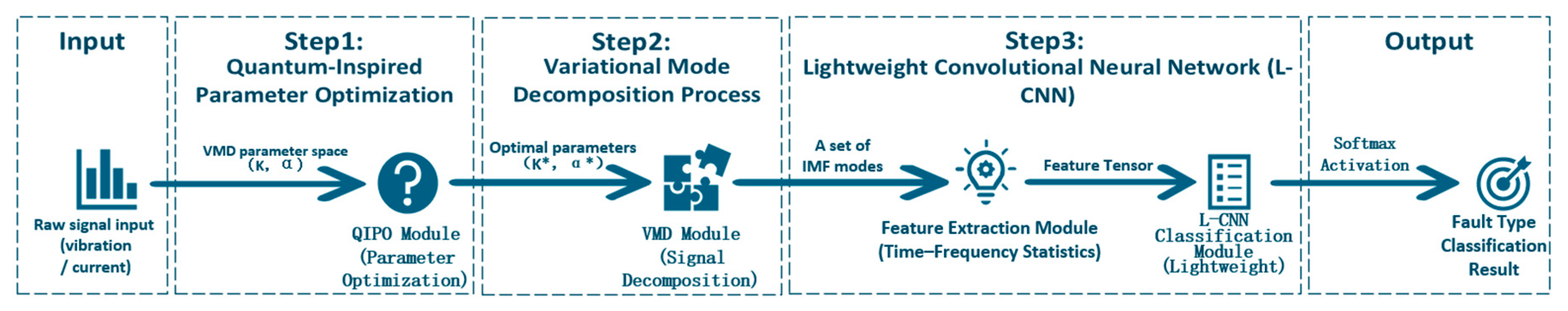
Figure 2.
Architecture of the L-CNN.
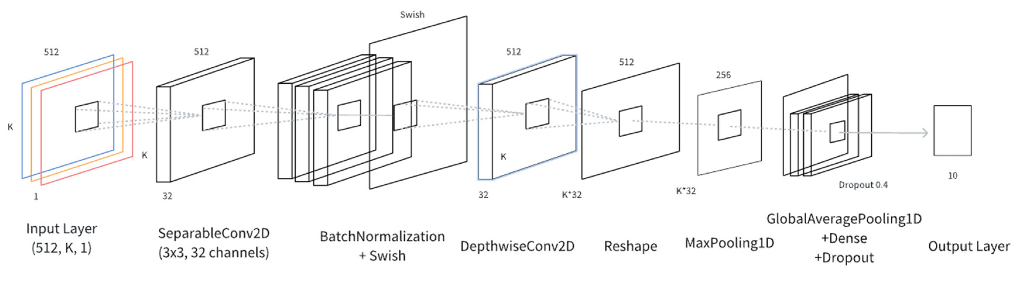
Figure 3.
(a) Distribution of reward values and their 10-iteration moving average (red curve) across iterations. (b) VMD decomposition energy and its 10-iteration moving average (purple curve) during optimization.
Figure 3.
(a) Distribution of reward values and their 10-iteration moving average (red curve) across iterations. (b) VMD decomposition energy and its 10-iteration moving average (purple curve) during optimization.
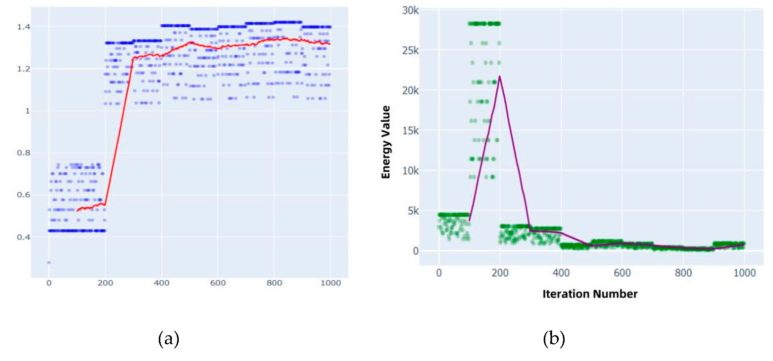
Figure 4.
(a) Evolution of the probability distribution for the number of VMD modes K during optimization.(b) Evolution of the probability distribution for the penalty factor α over iterations.
Figure 4.
(a) Evolution of the probability distribution for the number of VMD modes K during optimization.(b) Evolution of the probability distribution for the penalty factor α over iterations.
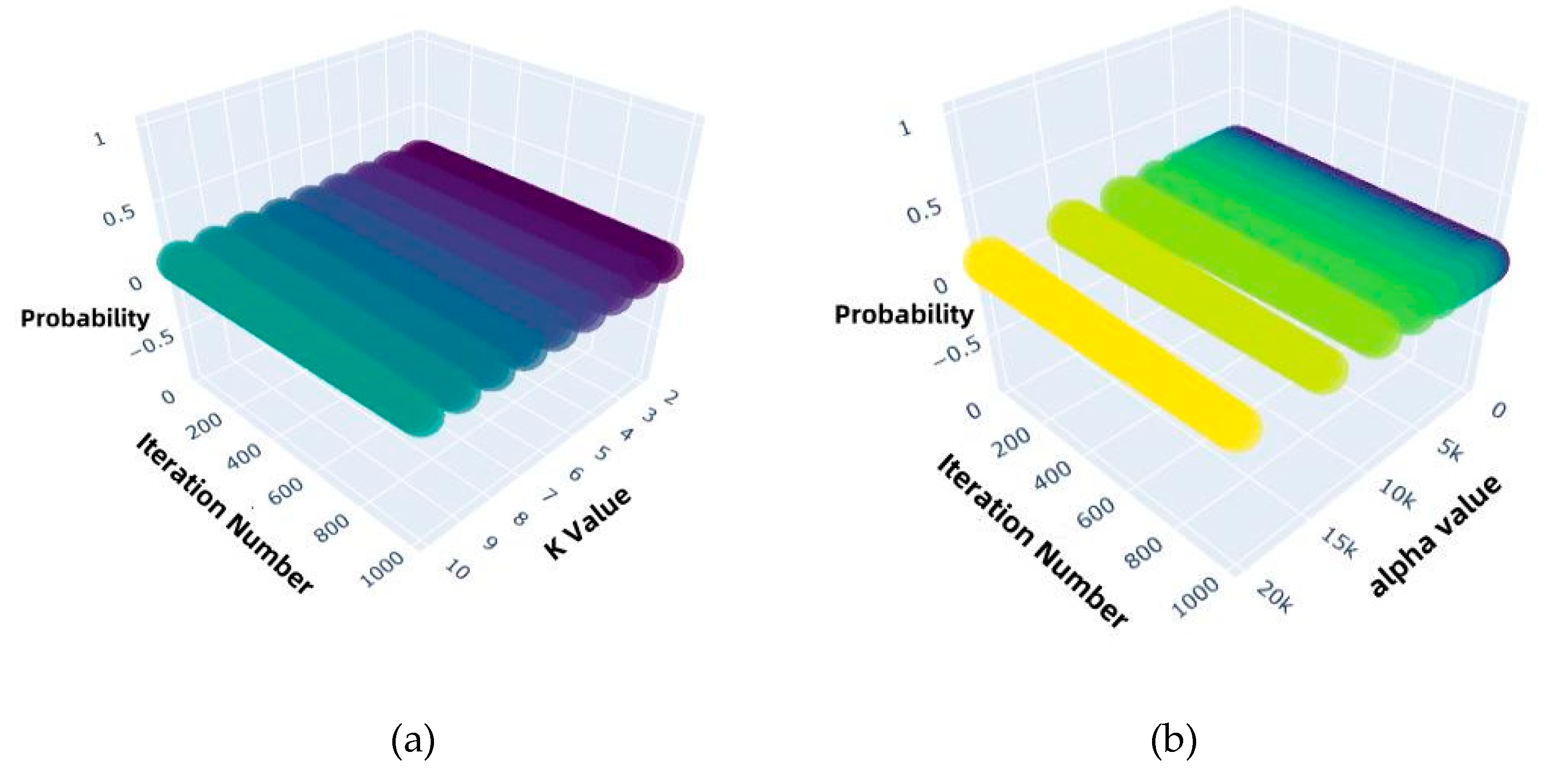
Figure 5.
The heat map of energy distribution of different fault type samples across each IMF component.
Figure 5.
The heat map of energy distribution of different fault type samples across each IMF component.
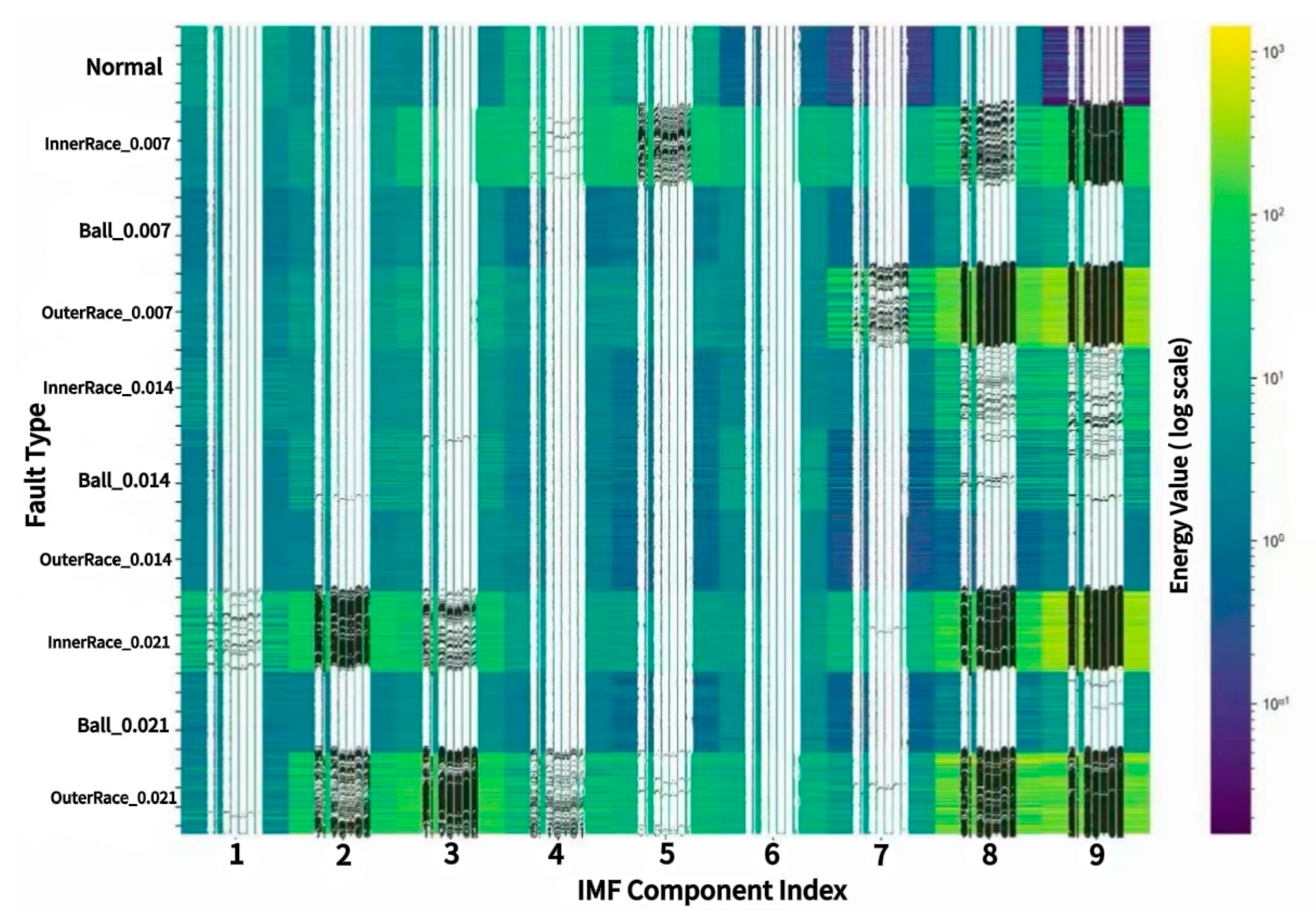
Figure 6.
Energy distribution heatmap of IMF components for different fault types.
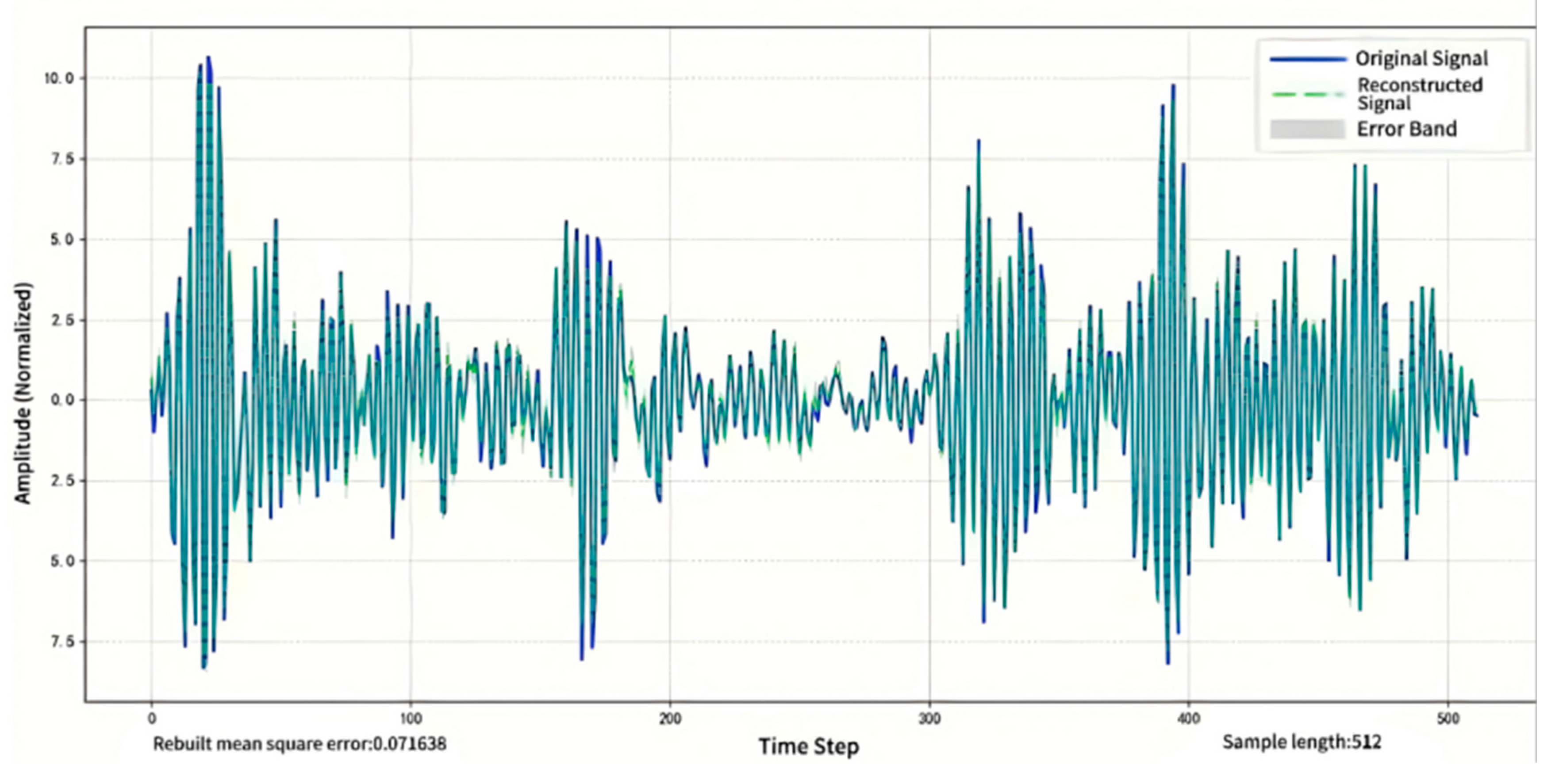
Figure 7.
Loss and accuracy curves during L-CNN training.
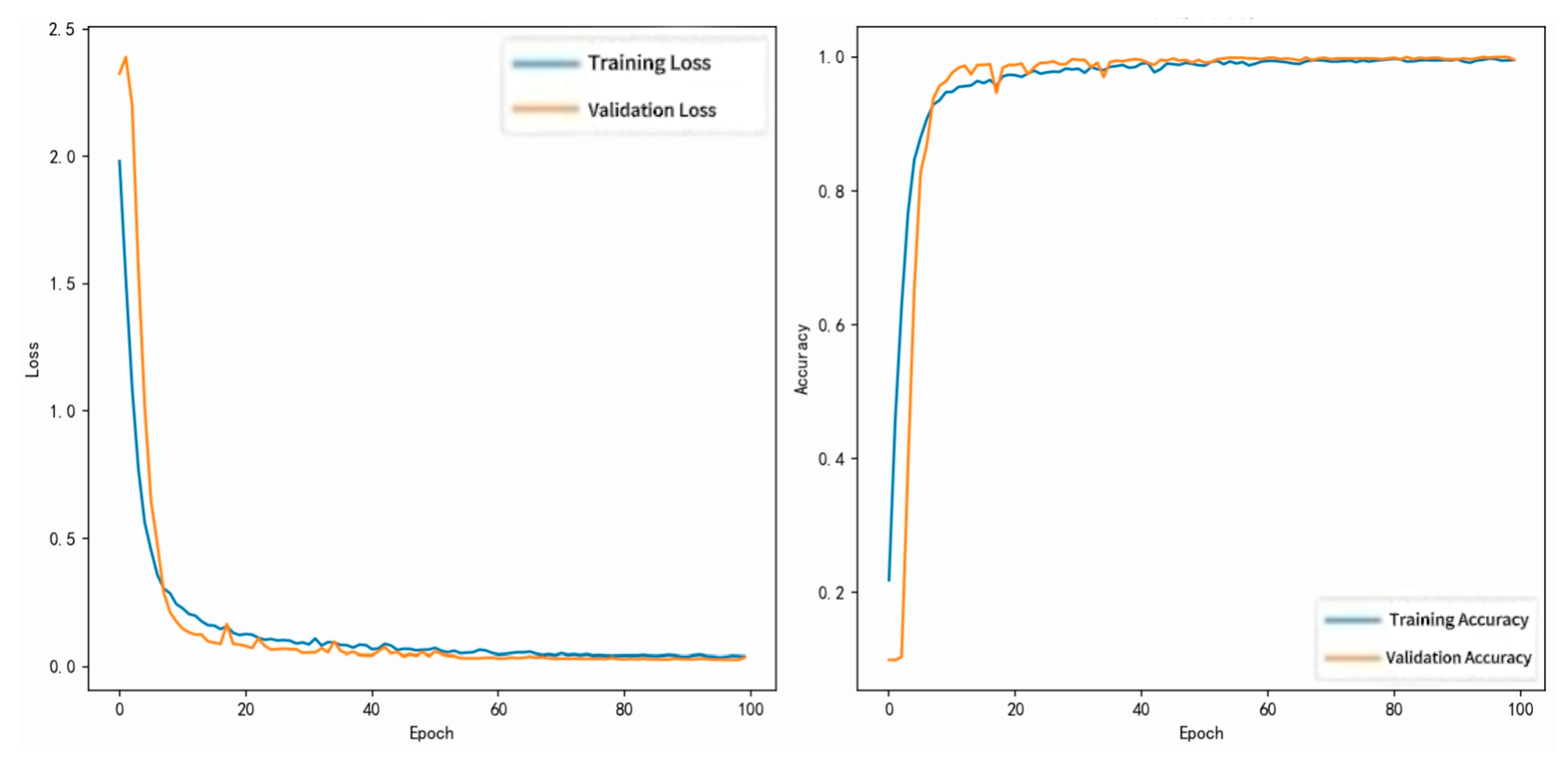
Figure 8.
ROC curves for L-CNN on multi-class fault classification.
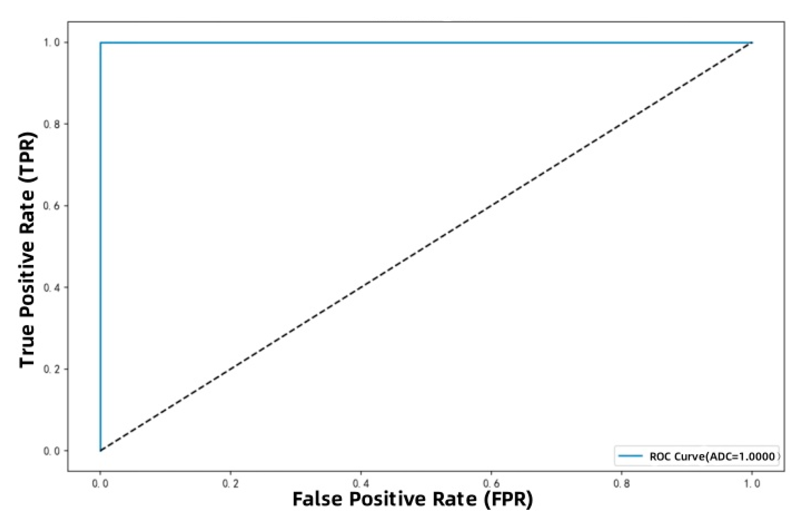
Figure 9.
PR curves during L-CNN training.
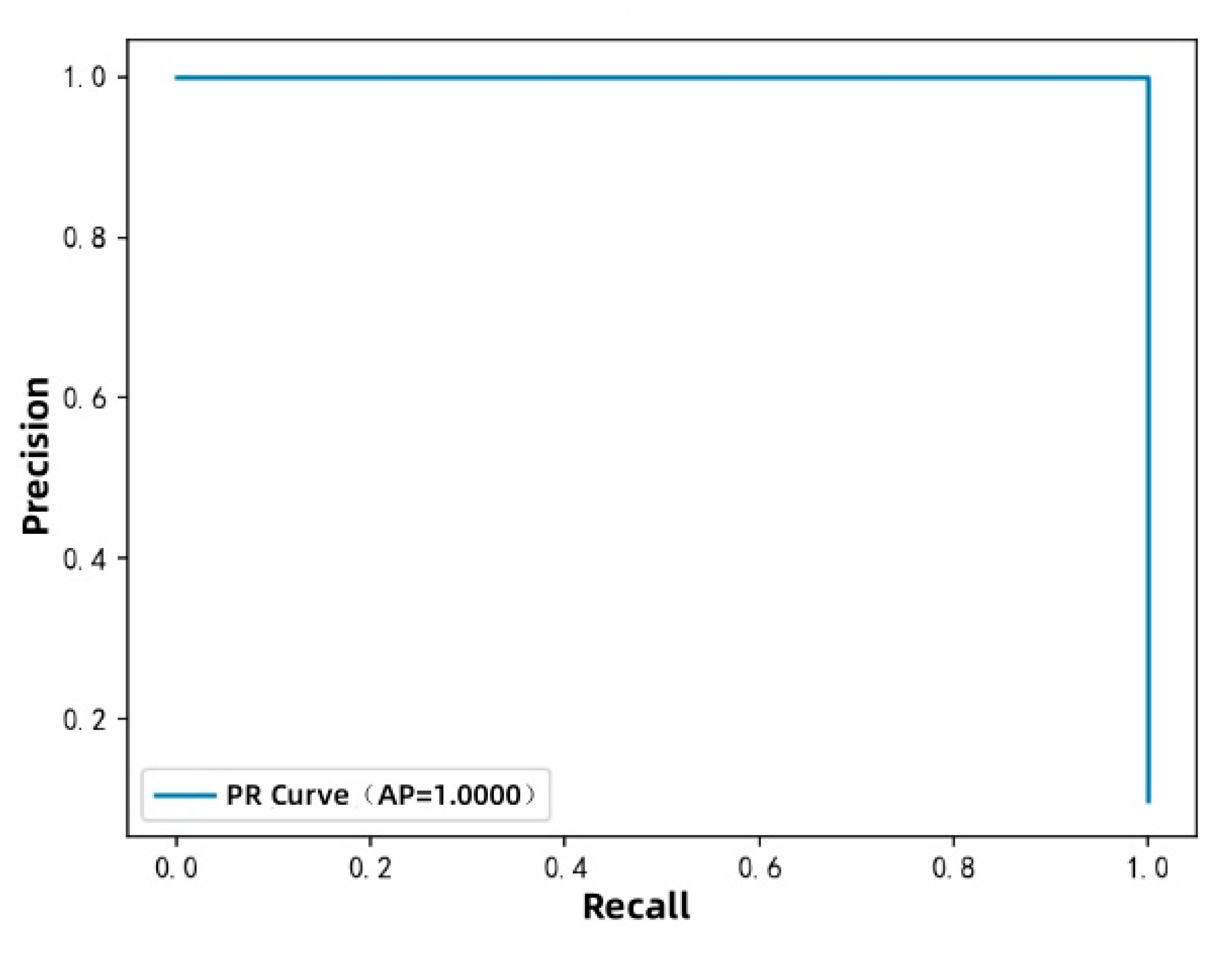
Figure 10.
Inference latency distribution of L-CNN on embedded platform.
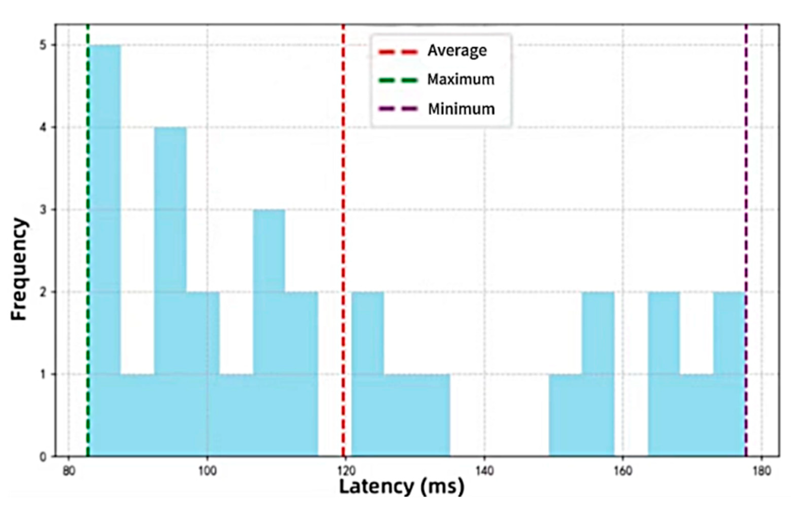
Figure 11.
Confusion matrix for L-CNN on 10-class bearing fault diagnosis.
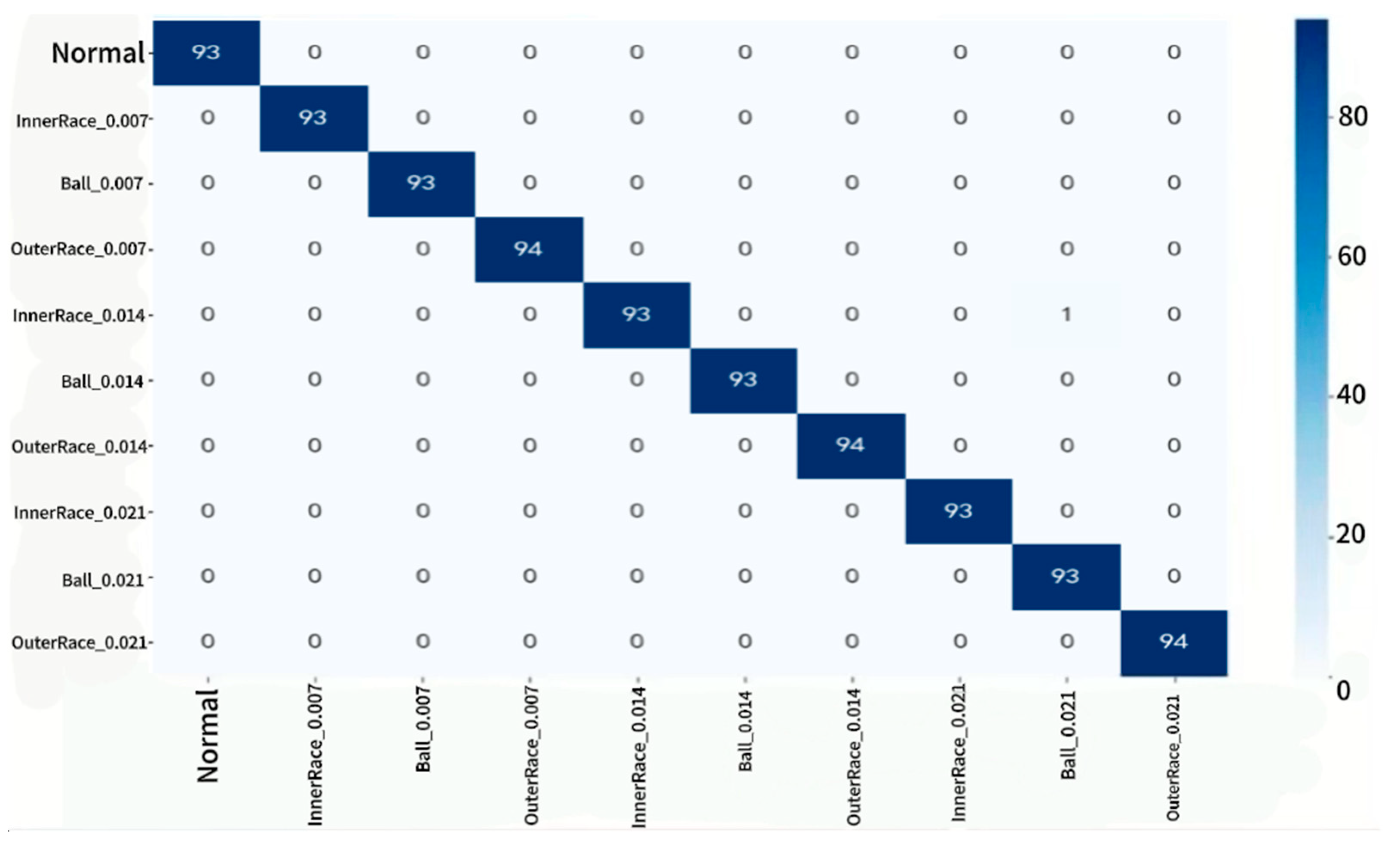
Table 1.
Layer-wise Configuration of L-CNN.
| Layer Type | Layer Parameters | Output Features |
| Input Layer | (512, K, 1) | (512, K, 1) |
| SeparableConv2D | (3,3), 32 channels, padding=‘same’ | (512, K, 32) |
| BatchNormalization | - | (512, K, 32) |
| Activation | swish | (512, K, 32) |
| DepthwiseConv2D | (3,3), padding=‘same’ | (512, K, 32) |
| Reshape | to 1D | (512, K32) |
| MaxPooling1D | pool_size=2 | (256, K32) |
| Channel Attention Mechanism | - | (256, K32) |
| GlobalAveragePooling1D | - | K32 |
| Dense | 128 units, swish activation, l2 regularization |
128 |
| Dropout | 0.4 | 128 |
| Dense (Output Layer) | 10 units, softmax activation | 10 |
Table 3.
Details of the CWRU Bearing Dataset.
| Fault Type | Damage Size | Sample Count | Signal Characteristics |
| Normal | – | 93 | Stationary vibration, no significant impulsive components |
| Inner Race Fault | 0.007 inch | 93 | High-frequency shocks, characteristic frequency ≈ 162 Hz |
| Inner Race Fault | 0.014 inch | 93 | Stronger impacts, wider frequency band |
| Inner Race Fault | 0.021 inch | 94 | Intense impact response, multiple harmonic components |
| Roller Fault | 0.007 inch | 93 | Periodic intermittent impacts, characteristic ≈ 108 Hz |
| Roller Fault | 0.014 inch | 94 | Shortened impact intervals, concentrated energy |
| Roller Fault | 0.021 inch | 93 | Wideband vibration, with harmonics |
| Outer Race Fault | 0.007 inch | 94 | Low-frequency impacts, characteristic frequency ≈ 60 Hz |
| Outer Race Fault | 0.014 inch | 93 | Energy shift toward low frequency |
| Outer Race Fault | 0.021 inch | 93 | Strong low-frequency vibration, significant noise suppression |
Table 4.
Performance Comparison of QDVMD-LCNN and Baseline Models .
| Method | Accuracy | Parameter Count | FLOPs (G) |
| Traditional CNN | 95.12% | 668,787 | 0.718 |
| GJO-VMD + CNN | 97.80% | – | – |
| Lite CNN | 99.97% | 903,000 | 0.0177 |
| ResNet50 | 99.97% | 47,187,000 | 0.718 |
| MADCNN | 99.70% | – | – |
| QDVMD-LCNN | 99.95% | 55,000 | 0.00104 |
Table 5.
Dataset Details of the Power System (IEEE PES Fault Database).
| Category | Fault Types | Number of Samples | Sampling Frequency | Fault Location |
| Details | Line-to-line (LL), single line-to-ground (LG) faults (including 0 Ω / 50 Ω / 100 Ω transition resistances) | 12,001 sets | 1kHz | Midpoint of transmission line |
Table 6.
Dataset Details of the New Energy Vehicle Drivetrain System – Multimodal Dataset.
| Category | Operating Conditions Covered | Number of Samples | Sample Ratio |
| Details | Urban driving (NEDC) and highway conditions (WLTC) | 22,000 sets | Normal : Fault = 1:1 |
Table 7.
Comparison of the Proposed Method and Other Algorithms on the IEEE PES Power Fault Dataset.
Table 7.
Comparison of the Proposed Method and Other Algorithms on the IEEE PES Power Fault Dataset.
| Algorithm | precision | recall | f1-score |
| WA-SVM | 0.8282 | 0.7484 | 0.7245 |
| IVMD-DCNN | 0.9561 | 0.9534 | 0.9531 |
| Wa-Bagging | 0.9798 | 0.9792 | 0.9791 |
| Traditional_vmd-wvd-cnn | 0.9539 | 0.9459 | 0.9455 |
| QDVMD-LCNN | 0.9965 | 0.9964 | 0.9966 |
Table 8.
Comparison of the Proposed Method and Other Algorithms on the NEV New Energy Vehicle Dataset.
Table 8.
Comparison of the Proposed Method and Other Algorithms on the NEV New Energy Vehicle Dataset.
| Algorithm | precision | recall | f1-score |
| Wa-Svm | 0.9837 | 0.9836 | 0.9836 |
| Traditional_vmd-wvd-cnn | 0.4594 | 0.5477 | 0.4811 |
| QDVMD-LCNN | 0.9873 | 0.9873 | 0.9872 |
Disclaimer/Publisher’s Note: The statements, opinions and data contained in all publications are solely those of the individual author(s) and contributor(s) and not of MDPI and/or the editor(s). MDPI and/or the editor(s) disclaim responsibility for any injury to people or property resulting from any ideas, methods, instructions or products referred to in the content. |
© 2025 by the authors. Licensee MDPI, Basel, Switzerland. This article is an open access article distributed under the terms and conditions of the Creative Commons Attribution (CC BY) license (http://creativecommons.org/licenses/by/4.0/).
Copyright: This open access article is published under a Creative Commons CC BY 4.0 license, which permit the free download, distribution, and reuse, provided that the author and preprint are cited in any reuse.


