3. Methods
The quantification of refractive index
along the line of the sight must be precisely addressed when the beam ray experiences different refraction conditions with respect to the atmospheric variations in each medium. This might occur several times during time of the measurement. Therefore, the error model for optimization of the systematic error caused by atmospheric effects, from Equation 1, can be rewritten as follows:
where,
refers to the refracted range, refracted vertical angle and refracted horizontal angle, respectively. To reduce the complexity of the problem, it was suggested that accurate observations of atmospheric conditions at both terminals of the sight line are measured, and then the mean calculation of the refractive index is applied as the real refractive index [
1]. These correction factors are referred to as the first velocity correction, and its comparison with the reference refractive index
is the second velocity correction for range measurements. The second velocity correction is typically implemented in order to ensure the required precision for estimation of refractive index (at least better than
). Note, in most cases, for either end, the defaulted value within the instrument is assumed as the reference refractive index [
3,
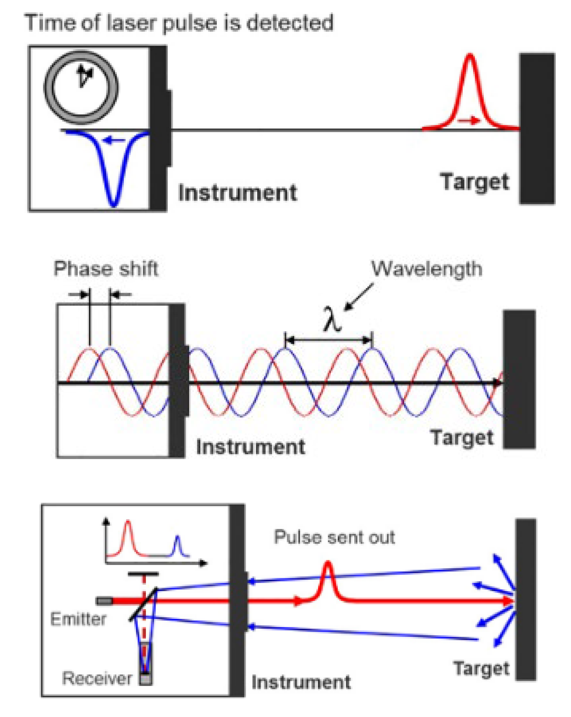
31]. Since TOF is the scanning mechanism behind long-range scanners for range measurements, the first and second velocity correction factors must be simultaneously substantiated after precise observations of atmospheric variables, through a physical refractive index model.
As discussed earlier, there are a number of physical refractive index models. Among all sets of calculations, Ciddor’s parameterisations provide more robust results than the previous versions [
22,
23]. Under this formulation, it was noticed that this setup is appropriate over a broader range of wavelengths (within
). Additionally, Ciddor physical model supports more flexibilities under extreme environmental conditions [
26,
27]. To implement Ciddor’s refraction model, the three following steps must be implemented:
- 1.
The first step is to differentiate the phase refractive indices
1 of standard air
2 and water vapor
as the function of the wavelength and irrespective of atmospheric variables:
Here, the wave number in is reciprocal of wavelength (.
The correction factor = is considered (dimensionless).
The group refractive indices are also computed as below:
- 2.
Next step is to compute the refractive index based on the atmospheric conditions, density components of the dry air and , and the moist air and with corresponding values of compressibility of air COM:
where,
is temperature
is the pressure
, is the water vapor pressure component of the air depending on the humidity
(as three major atmospheric components for this contribution),
is the molar mass of water vapour containing
of
,
is the molar mass of water vapor
, and
is the gas constant (
. Then, compressibility
based on each air conditions - either standard dry air or pure water vapor - are computed:
Here, is the temperature in
- 3.
Ultimately, the combined evaluation of both refractive indices - under dry air and water vapor component - is determined by [
22,
23]:
Ciddor’s parameterisations have been later adopted by the International Association of Geodesy (IAG) in 1999, as the standard equation for calculating index of refraction for geodetic instruments operating within the visible and near infrared waves [
24]. The principle is referred to as the Closed Formula model. IAG’s proposal provides more accurate results under more extreme temperature, pressure and humidity conditions through simplification of the Ciddor’s principles and less computational skills. Thus, the methods to achieve the group refractive index
as a function of
in
is straightforward as follows:
Afterwards, the group refractive index
under either standard air condition or water vapour is computed:
Given each model, either the Ciddor or Closed Formula, three spatial variations of the refractive index
in 3D Cartesian coordinates can be parameterised as the gradient of the refractive index
:
The elements on the horizontal plane
affecting the horizontal directions are called horizontal gradients of refraction, while
refers to the vertical gradient of refractive index impacting the vertical directions. Therefore, the gradient of refractive index is rewritten as the function of the atmospheric variables:
where,
or
and
are horizontal and vertical gradient of air temperature, atmospheric pressure and humidity of air, respectively [
32].
To investigate different gradient components of the refractive index, the stable stratification of the atmosphere - based on air temperature - is sometimes supposed in analytical studies. The stable stratification condition is defined when air temperature decreases gradually with height. In contrast, unstable stratification occurs when the air temperature decreases rapidly with height, or changes irregularly with height. The vertical temperature gradient is generally described as the variation of temperature vertically under stable stratification conditions. In the following studies [
29,
33], different layers of the atmosphere - with respect to the height from ground level, from
(directly above the ground) to over
- were categorised, and the corresponding practices for computing the vertical temperature gradient were presented. In summary, vertical temperature gradients are substantially intense in the layers close to the ground surface within a range of
to
(between
and
) and drops to the small value
at the highest assumed level.
Alternatively, the variation of temperature horizontally or laterally, impacting the horizontal direction of refractive index is the horizontal temperature gradient. There have been several methodologies to determine the horizontal temperature gradient. For example, B. G. Bomford [
2] assumed that for an approximate distances of
horizontally and
vertically, with
temperature rise between the terminals, the difference in average horizontal temperature gradient is nearly
(i.e., the increase of
per kilometer in lateral difference). Another theory in the lowest layer of atmosphere – where a line of sight is two meters above the ground level with the vertical temperature gradient of
- the horizontal temperature gradient is checked, and it is assumed negligible.
Comparing these two gradients, the effect of atmospheric variables horizontally is trivial. Therefore, Equation 24 depicts the relationship between vertical gradient of refractive index
and the vertical temperature gradient
as well as the vertical pressure gradient
and vertical humidity gradient
[
27]:
As discussed earlier, the primary contributor to the vertical gradient of refraction is the vertical temperature gradient, with minimal influence from other vertical gradients. Further developments regarding the pressure and humidity vertical gradients are presented in
Appendix B.
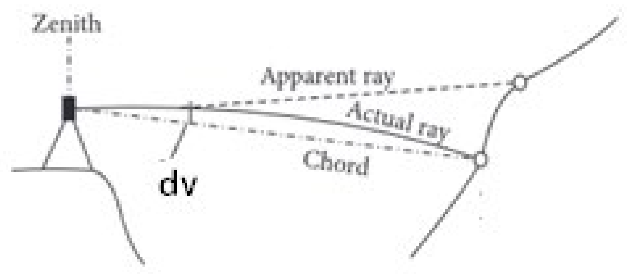
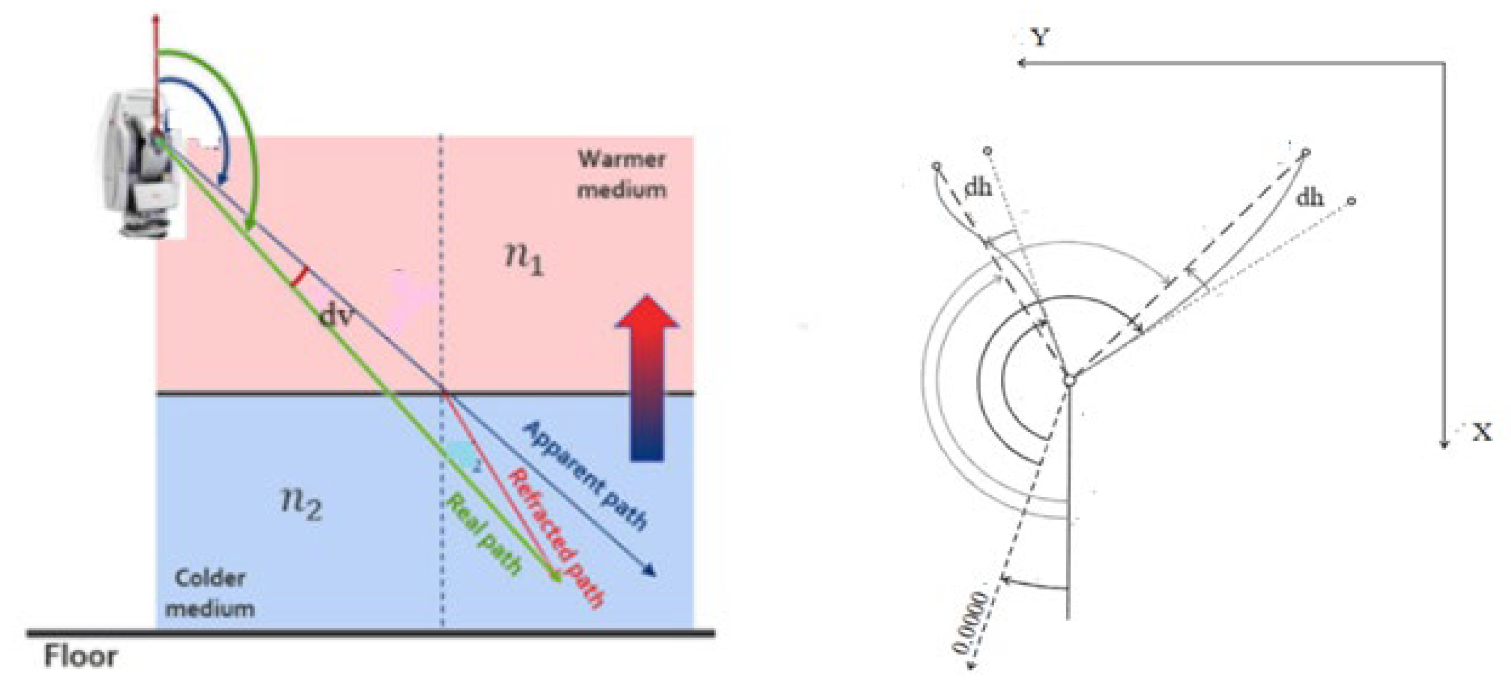
Consequently, under these assumptions, the corrected range
and corrected vertical angle
can be expressed in terms of the refracted range
and refracted vertical angle
, respectively. These are derived by integrating of the refractive index effects over the entire length of actual ray (observed range
) (
Figure 1):
Also, a refracted horizontal angle
is reparametrized in terms of horizontal gradient of refractive index
Accordingly, to achieve an optimal performance of the refractive index correction through a physical model, the refractive index is approximated by the averaged values obtained at both terminals of the line of sight
and
[
1]. This means that refractive index is expressed as (
Section 5.1):
However, the imposed simplification underestimates the potential non-linear vertical variations of the atmosphere along the actual ray path, as the laser beam experiences multiple refraction abnormalities when traversing different atmospheric layers. Therefore, in this research, a more accurate physical model is proposed to account for the varying vertical gradients of the refractive index along the propagation path – referred to as advanced physical refractive index model. According to Equation 25, it can be rewritten in the following expression:
where
represents the height profile along the laser path, with
being the counter that moves between
and
. The refractive index is approximated as the nonlinear function to the range rather than applying the mean value between two refractive indices:
Therefore, from Equation 26, the refracted vertical angle
can be (
Section 5.2):
Note, in either case, to guarantee millimetre- or sub-millimetre-accuracy for the observations, a precision of at least
must be accomplished for the estimation of refractive index [
1]. Then, it enables reducing sensitivity to the spatial variations in the refractive index and enhancing the overall accuracy of 3D point coordinates.
To represent refractivity along the entire line of sight, the illustrated techniques on physical model establish a reasonable relationship between environmental parameters (e.g., in-situ atmospheric recordings) and wave number (i.e., scanner wavelength) as the inputs, and the real-world refractivity along the beam path as the output. However, to achieve rigorous precision and consistency in TLS-based physical refractive index modeling, a hybrid physical-data-driven model is proposed as a follow-up. This hybrid model integrates results from the advanced physical model with a neural network approach, and its function is justified through field-validated outcomes from previously established physical models. It guarantees optimal millimeter-level accuracy in 3D point coordinates and enables consistency checks across two long-range scanners under varying atmospheric conditions (
Section 5.3).
In short, a neural network is a machine learning algorithm simulated from the structure of the human brain. It generally consists of a variety of layers from interconnected neurons, which each one collects the inputs and interacts with the result to the next consecutive layers to generate rigorous outputs. These neurons utilize certain mathematical algorithms and adjust internal weights during each training interval to minimize the prediction errors for both datasets, according to the received residuals [
34]. The minimization of residuals of 3D spherical coordinates signifies the lowest ultimate uncertainty for the 3D point coordinates (on the order of millimetre or sub-millimetre relative precision). It ultimately ensures the robust prediction by the most accurate output - refractive index and its spatial gradients along the laser path.
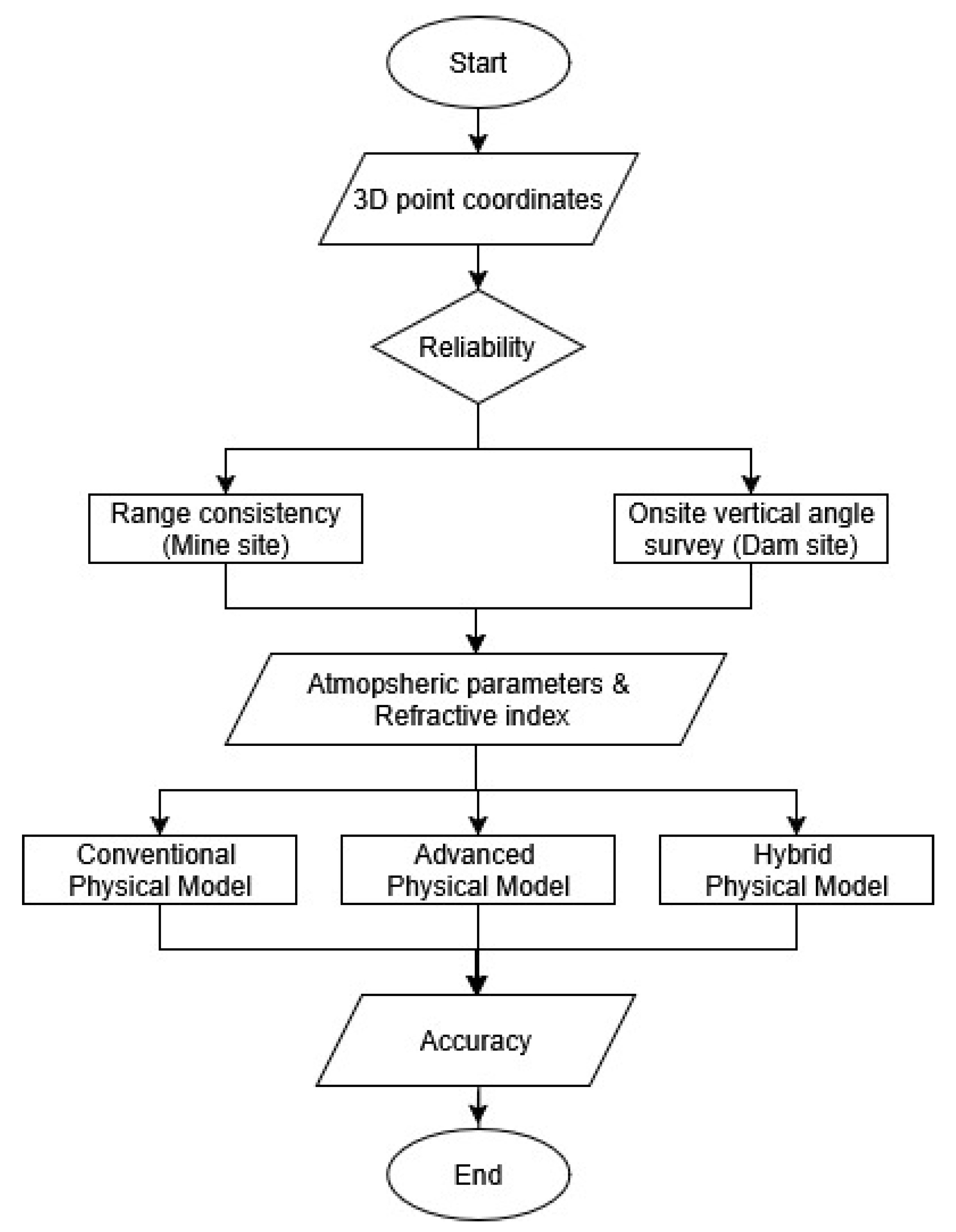
In summary, three different methods are tested to improve calibration uncertainty (
Table 1). To achieve high-precision calibration setups, two geodetic test fields, mine site and dam site, were established within a calibrated network using post-processed GPS control points and onsite terrestrial surveys, delivering
accuracy in range and
in vertical angle observations. In addition, in-situ atmospheric observations were collected at each scan station to improve refractive index modeling. Using the proposed approaches, refractive index estimation with high precision is implemented prior to 3D point coordinate accuracy assessments.
4. Data Experiments
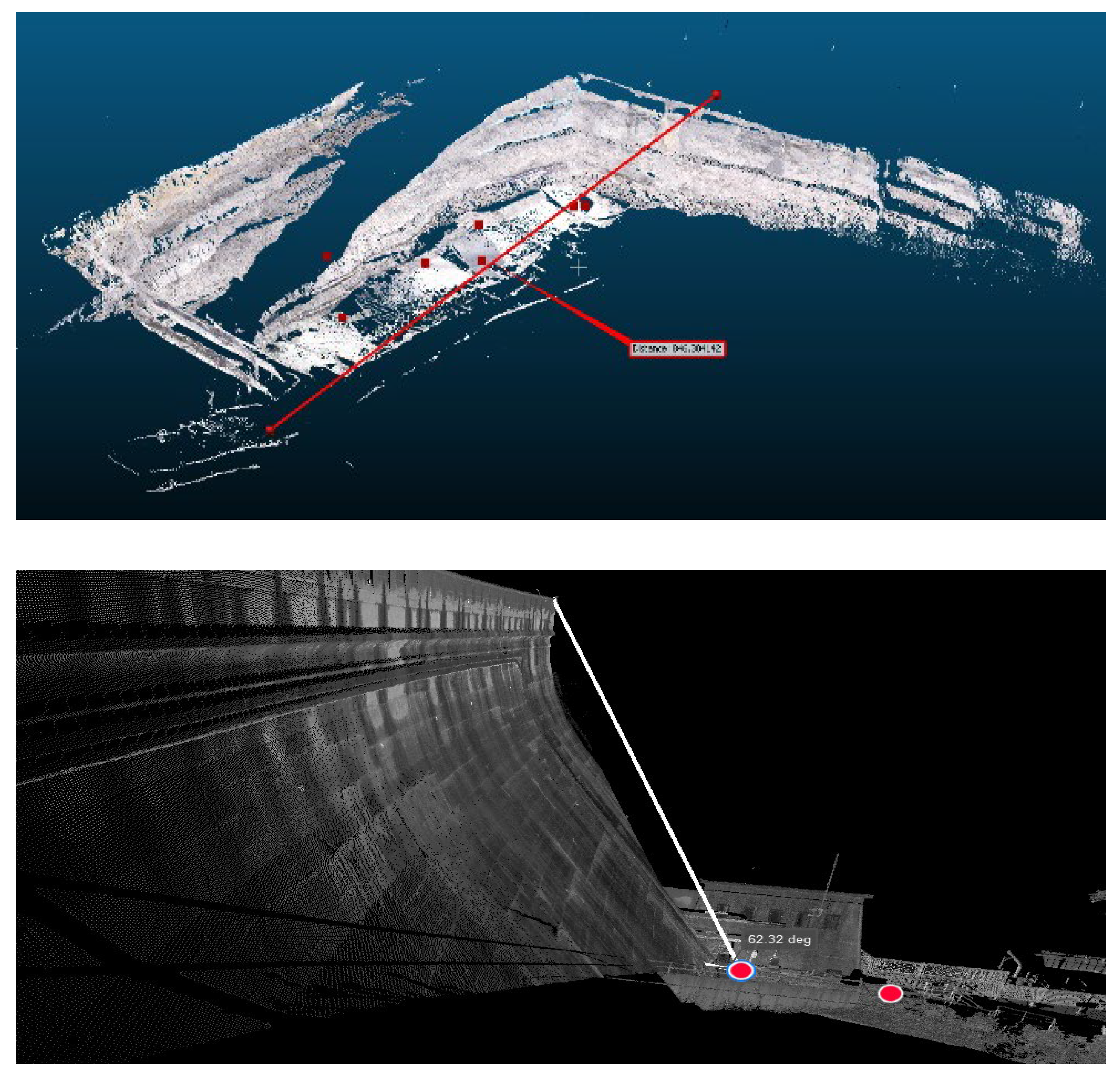
The above theoretical developments were tested on real case studies acquired from a mine site and a dam site (
Figure 5). The mine site experimental test field examines long-range scanning with the maximum range of
, while the dam site experimental test field provides the flexibility for investigation of a steep vertical angle from the bottom of the dam to the dam crest (maximum vertical angle captured on-the-site is
). At the mine site, the data field capture was set up within a calibrated network using eight GPS control points distributed at different elevations across the site (red points shown in
Figure 5). The reason for distributing the control points at varying heights is to investigate the varying vertical gradient of refractive indices across different horizontal stratifications of the atmosphere for the advanced hybrid model (e.g.,
for Station 1,
for Station 2, and
for Station 3 (
Table A2 in
Appendix C)). At the dam site, a Leica Nova MS60 MultiStation was used to measure
black and white targets established on the semi-vertical dam walls (i.e., range and angular accuracies of the Leica MS60 are
and
, respectively
3).
Furthermore, GPS control points for the mine site were collected on-the-site using static mode and have been post processed after the field collection at the office to reduce to the highest accuracy within
to
. GPS control coordinates and survey control marks for both datasets are listed in
Table A2 and
Table A3 in the
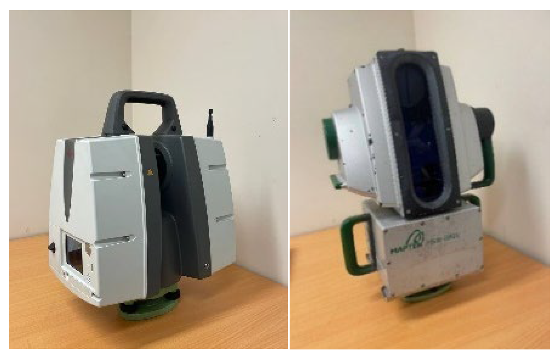
Appendix C, respectively. For scanning, two long-range scanners - Leica ScanStation P50 (measurement range
) and Maptek I-Site 8820 (measurement range
) were employed (
Figure 6), and
Table 2 indicates technical specifications of the scanners, reported by the manufacturers, and contains the scanning characteristics used in this research.
The datasets from three nominal scanner stations were captured under identical filed instructions on the 10th of December 2024 (mine site) and the 15th of February 2025 (dam site), during working hours from
to
. During scanning, long-range mode within the scanners was activated, and all default correction factors including instrumental atmospheric refraction were switched off. At least two scans from each station with the maximum possible instrumental resolution were acquired (
Table 2) (i.e., each with different horizontal orientation).
The environmental conditions of the sites were precisely recorded during scanning time using a Kerstal 2500 weather meter sensor. The reported precisions for the temperature and pressure are
and
, respectively. The link regarding technical provisions of the thermometer was provided
6.
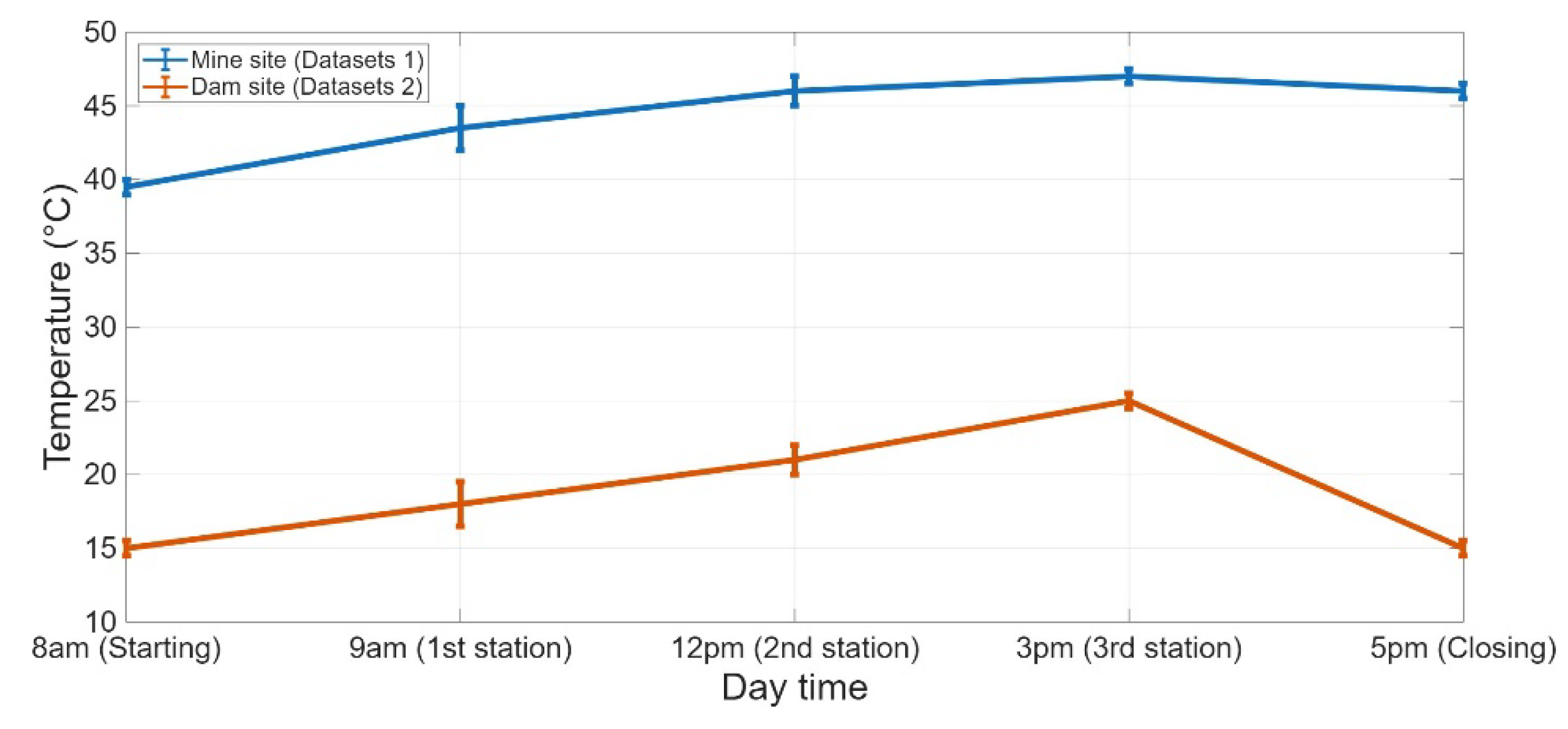
Figure 7 compares two different temperature recordings across two geodetic sites.
To optimally comprehend the level of atmospheric variations across the field, the atmospheric recordings were achieved by at least two weather meter sensors, and the measurements were initiated from the surrounding of each scanner station and continued onsite close to every target location – from the nearest to furthest target location - during scanning time. For example, at when the scanner was set up at the first station, the observed temperature close to the station was at the mine site. Across the entire test field, the temperature varied by relative to the station’s record (i.e., the atmospheric data attached to each scanner station). By , however, the temperature had increased to across the whole site. In addition to temperature recordings, the atmospheric pressure of both sites was observed using the same sensor. Compared to temperature, the atmospheric pressure across the areas was considerably stable during the observation time (and for the mine and dam site, respectively).
5. Data Analysis and Discussions
The datasets from both scanners were collected in the calibrated test field under uncontrolled environmental conditions. For the mine site dataset, the range consistency calibration method is implemented, while for the dam site dataset, on-the-site calibrated angle measurements using terrestrial surveying are undertaken. In short, the range consistency method provides the geometric accuracy as the result of verifying the ranges between each pair of corresponding control points remain invariant across multiple scanner stations [
35,
36,
37]. The existence of eight control points for the mine site dataset delivers
Euclidean ranges for each station, and 14 targets for the dam site dataset offer the same number of angles per scanner setup. Total redundancy for each dataset is six times those numbers (depending on the number of scans). Then, the following step is the accuracy assessment of different proposed physical models in long-range terrestrial laser scanning.
After importing scanned data for each instrument separately using Maptek PointStudio 2024.1.1
7 and Leica Register 360 software
8, each of the corresponding control points was manually selected, and spherical coordinates using the developed MATLAB codes were determined. There was no software registration implemented for the calibration arrangement. The reason is that either software registration (automatic point-to-point or cloud-to-cloud) or manual registration imposes an additional root mean square error (RMSE), originated from the software comparison between the clouds. Importantly, the in-situ atmospheric recordings were attached to each scanner station (
Figure 7).
Primarily, the reliability of the datasets is examined using hypothesis tests. The objective is to eliminate the measurements containing outliers due to the manual target selection and reducing the potential propagation of noise, which might otherwise degrade the precision of refractive index estimation, leading to lower accuracy of 3D point coordinates. The hypothesis test compares the weighted
sum of the squares of the residuals
against the chi-square distribution
, with redundancy numbers
, and the significance level
. Given the assumed significance level at least
for both datasets and corresponding redundancy, the test fails if
is greater than critical value of the distribution (outliers exist in the measurements), or if this is smaller than the critical value, the test passes (better precision than prescribed) [
38] (where,
and
are residuals and standard deviation, respectively).
The underlying assumption of the hypothesis test is that outliers can be detected in a reasonable manner (internal reliability), and the impacts of other undetected outliers are insignificant (external reliability). Then, given either physical refractive index model (the Ciddor or the Closed Formula model), the refractive index is determined at the maximum level of precision, optimally reflecting the real-world atmospheric conditions along the sightline. Subsequently, using Equations either 25, 26 or 28, the estimated precision of the refractive index directly affects the accuracy of the 3D spherical coordinates. The uncertainty of the 3D Cartesian coordinates
is evaluated using the principle of propagation error, representing the posteriori accuracy of the advanced model - whether physically or hybrid:
Here,
represent the posteriori accuracy of the 3D spherical coordinates. However, the accuracy assessment is interpreted as relative precision, given the accuracy of the control network
and
). Note that identical data analysis procedures are followed for both datasets.
Figure 8 highlights a broad summary of the proposed calibration methodologies, considering the mentioned criteria.
5.1. Physical Refractive Index Model: Conventional Approach
The mine site dataset examines long-range scanning within a calibrated network through a distribution of eight control points. To initiate the data analysis, the computed inter-target ranges from selected targets in each station’s point cloud are determined and validated against control points through a range consistency method (i.e., a total number of 168 ranges for the entire network). The range consistency calibration method ensures that the ranges between each pair of corresponding control points in the scanned data remain consistent across different scanner stations [
35,
36,
37].
For pre-processing of the physical model, reliability test on selected targets is recognized (using the hypothesis test Equation 32), resulting in 18 measurements for Leica ScanStation P50 and 12 measurements for Maptek I-Site 8820 being detected as the outliers and eliminated from the dataset.
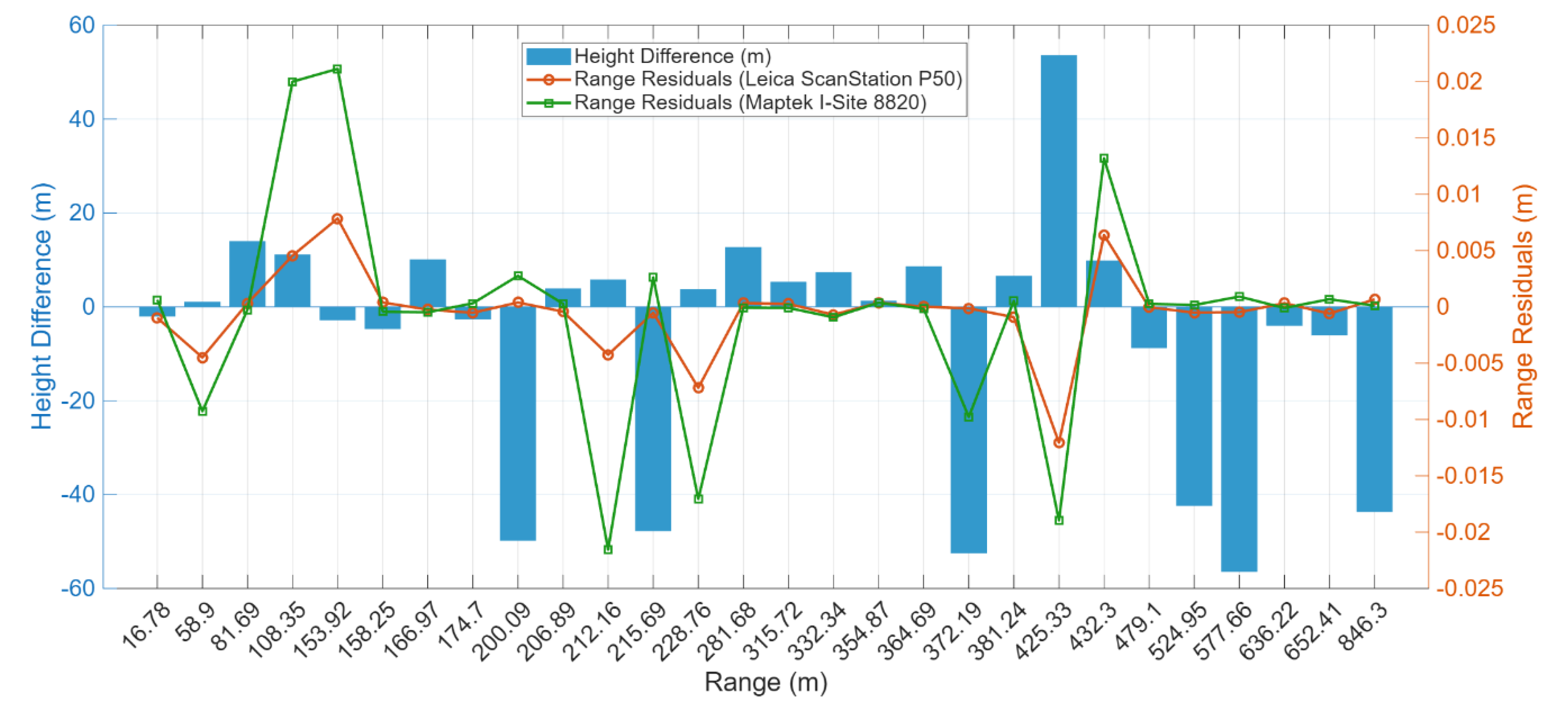
Figure 9 shows the results of comparing each pair of control ranges with the average residuals, considering their height differences (i.e., the average ranges are derived from observations made at multiple scanner stations).
The comparison above underlines that after applying the lowest significance level for hypothesis test (
), the residuals experience the noticeable variations. However, the obtained standard deviations of the measured ranges are
for the Leica ScanStation P50 and
for the Maptek I-Site 8820. Note, with the Maptek device, the larger standard deviation had been anticipated since the scanner has been operated in open pit mining sites and has not recently been under the uncertainty assessment. Additionally, the nonlinear relationship between the ranges and the residuals, for both scanners, highlights the complexity of atmospheric modelling for long-range terrestrial laser scanning. To date, conventional refractive index correction models for range measurements have typically been assumed to be linear, based on the relative consistency of the refractive index along a horizontal path, using the mean value from both ends of the sightline (Equations 25 and 28) [
1,
27].
The following reasons elaborate on the limitations of the conventional approach of the physical model. Firstly, vertical stratifications of atmospheric air conditions are substantiated and play a vital role in the atmospheric correction modelling of terrestrial laser scanners [
29,
33]. M. Sabzali et al. [
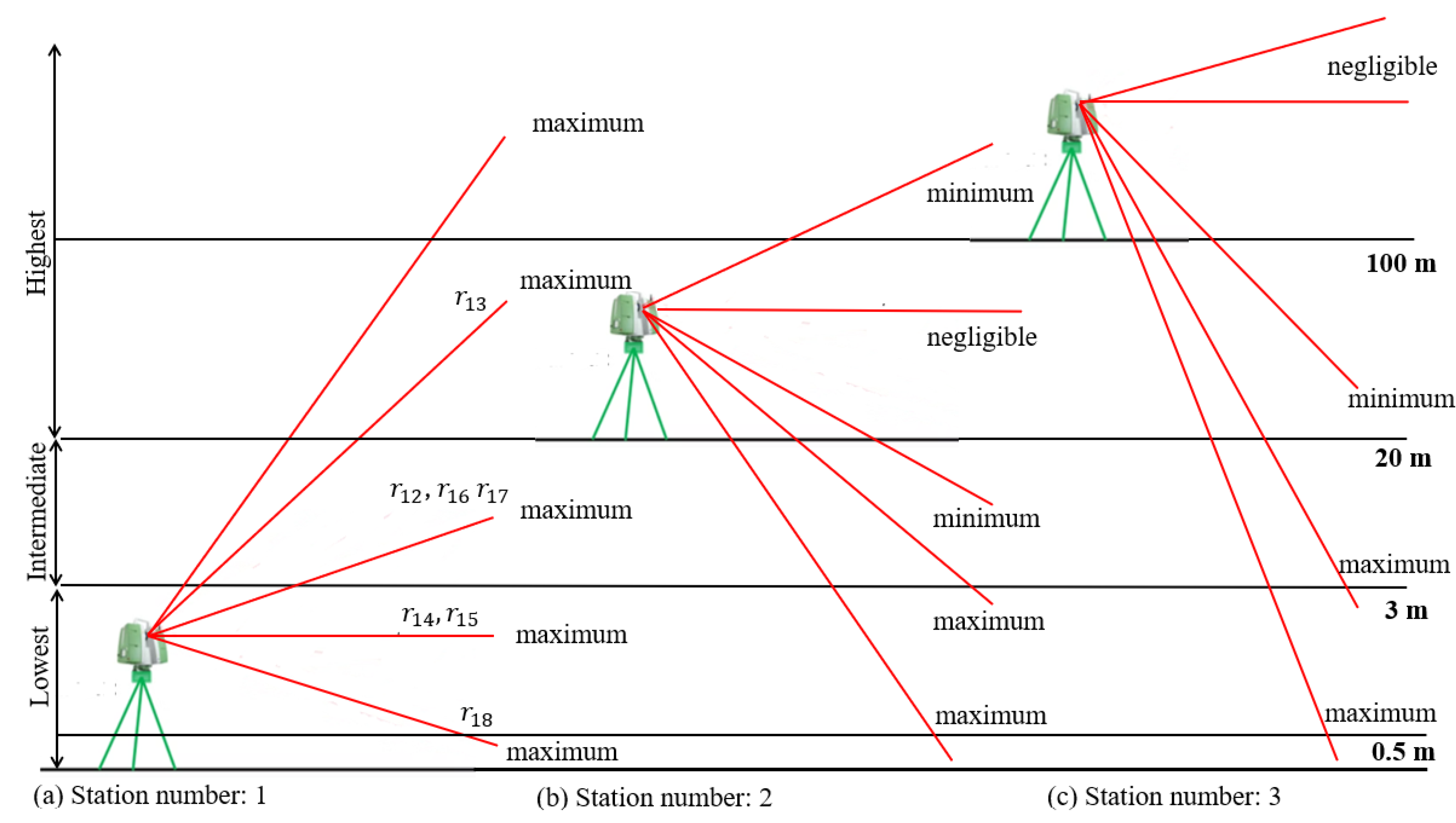
29] introduced different horizontal layers for the atmosphere depending on the height from ground level, according to the vertically stratified atmosphere. These layers commence from the layer closest to the ground surface, from zero to
(lowest layer, with the most influential variations in terms of atmospheric conditions),
(intermediate layer),
, and above
(highest layer, with the least influence in terms of atmospheric variations) (
Figure 6). It is acknowledged that the vertical variation of the atmosphere does not remain stable for the laser path passing within those layers, particularly for vertical temperature gradients. This vertical stratification of the atmosphere is a key consideration for improving current TLS atmospheric correction models. Due to the extended vertical field of view of terrestrial laser scanners (
Table 1), a large number of points are observed close to or at the zenith and nadir when the vertical field of view is maximized, dissimilar to the terrestrial surveying in which more points are captured through the limited vertical field of view near the horizon. Therefore, the observed ranges from terrestrial laser scanners experience varying atmospheric gradients along the path - the varying vertical gradient of refractive index - impacting not only the range but also the vertical angle at different horizontal layers of the atmosphere.
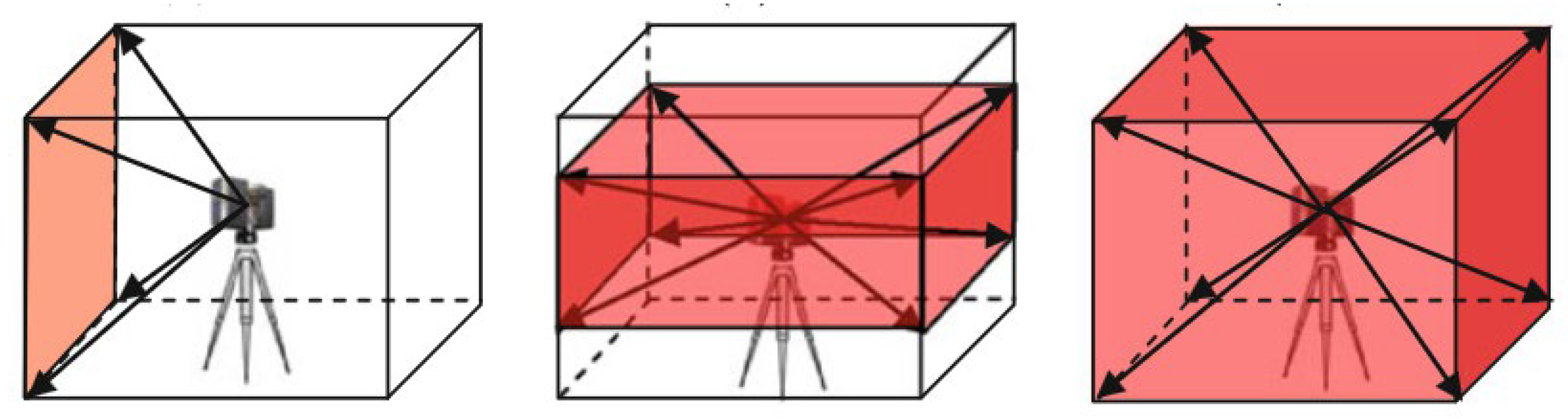
Figure 6.
Different conditions of refractive index modelling in TLS. Note, scale is not preserved in this figure (The list of control points is available in
Table A2 and
Table A4 in
Appendix C).
Figure 6.
Different conditions of refractive index modelling in TLS. Note, scale is not preserved in this figure (The list of control points is available in
Table A2 and
Table A4 in
Appendix C).
Thus, points at different height levels receive variable residuals, regardless of their measured ranges. For instance, three peak residuals correspond to different height differences and range observations (i.e.,
for the
,
for
and
for
). The first two are located within short- and mid-range observation, but their height differences indicate that both terminals of these lengths lie within the lowest atmospheric layer (
to
), and between the lowest and the intermediate atmospheric layers, respectively (
). Whereas, for the latter pair of points, the travelling path extends from the lowest to the highest atmospheric layer. Hence, the sightline travels from the layers close to the ground, with substantially noticeable atmospheric variations, to the highest layer with considerably insignificant atmospheric influences (
Figure 6, condition (a)).
In contrast, each pair of points at the highest layer or above (
Figure 6, condition (b) and (c)), regardless of their elevation and range, is less affected by atmospheric components, such as the ranges
,
,
,
, and
encompassing varying height differences (
Table A4 in the
Appendix C). The minimum, maximum, and negligible cases, as shown in
Figure 6, represent the bounds of refractive index correction that must be applied in the advanced model.
Given the arguments above, Z-coordinates of points observed at greater vertical viewing angles relative to the station require more significant atmospheric corrections than those of the X- and Y-coordinates at similar angles (e.g.,
Figure 6, the maximum cases). Nevertheless, for the points observed at smaller vertical angles - such as those lying close to same horizontal atmospheric layer as the scanner station - the atmospheric correction is often negligible (e.g.,
Figure 6, negligible cases). This simplification leads to an underestimation of atmospheric effects in conventional surveying tasks.
To investigate the introduced sensitivity in the vertical direction, the second dataset from the dam site provides significant vertical angle variations from three nominated scanner stations - from the bottom of the dam wall (lowest layer of atmosphere) to the survey targets on the dam wall and the dam crest (highest layer of atmosphere). In this experiment, 14 survey targets were positioned within a shorter range of scanning but at the higher vertical viewing angle (ranging from
to
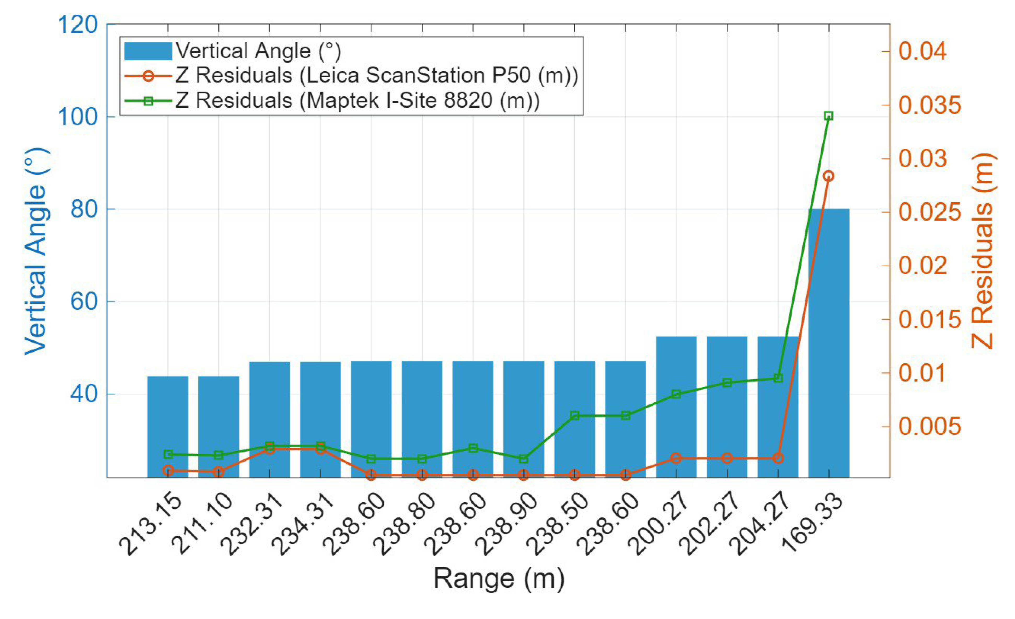
). The spherical coordinates were determined and validated against on-site survey data (i.e., in total, 84 vertical angles were derived for the entire network). After identifying seven and eleven outliers for the Leica ScanStation P50 and Maptek I-Site 8820, respectively, the results are depicted to compare the on-site surveyed vertical angles with the averaged Z-coordinate residuals (extracted from the average of measured coordinates), considering their measured ranges (
Figure 7).
Figure 7.
Control vertical angles, the ranges and the Z residuals (Dataset 2: dam site).
Figure 7.
Control vertical angles, the ranges and the Z residuals (Dataset 2: dam site).
The large vertical angles are associated with increased Z residuals (i.e., the standard deviations of the measured vertical angles are
for the Leica ScanStation P50 and
for the Maptek I-Site 8820). This outlines that observations at vertical angles beyond
exhibit greater sensitivity to atmospheric refraction effects than those within
(such as, Dataset 1: mine site).
Figure 6 illustrates the maximum cases of vertical gradient of refractive indices under condition (a), highlighting variations from the lowest to either the intermediate or the highest atmospheric layers.
In summary, when both ends of the sightline are located within the intermediate or higher atmospheric layers, refraction effects remain stable in relatively same horizontal layer (negligible cases;
Figure 6, conditions (b) and (c)). However, when either end of the sightline is placed within the intermediate or the lower atmospheric layers, the impact of atmospheric refraction becomes more significant and variant with respect to the vertical gradient of refractive index (maximum cases;
Figure 6, conditions (a) and (c)). Since terrestrial laser scanners typically transmit signals from one end of the sightline, the systematic error in relation to refractivity increases with the rise in the vertical angle from the horizontal plane in a nonlinear manner. This comparative discussion underscores the requirement for a physical model to account for the variability of temperature gradient along the laser path. The advanced physical model addresses this by incorporating varying vertical temperature gradients (Equations 29 and 31) for the points observed with a long-range baseline (greater than
) and a steep vertical angle (larger than
) [
27]. Consequently, the interdependence of spatial gradients of refractive index can be resolved through the high-precision determination of the refractive index along the travelling path [
28].
5.2. Physical Refractive Index Model: Advanced Approach
To overcome the limitations of the conventional physical model, the advanced physical model was introduced. The conventional approach of physical model, which assumes a uniform refractive index based on the average of two terminals, underestimates refraction impacts along the path with varying vertical gradients of refractive index, particularly at long ranges and steep vertical angles. The advanced model aims to incorporate vertical variations in refractive index, thus accounting for the nonlinear influence of refractivity along the propagation path (Equations 29 and 31). In practice, the model assumes different segmentations of a straight-line sight path through different atmospheric layers, with each layer characterized by its corresponding vertical temperature gradient and vertical refractive index gradient. This approach depicts the vertical stratification of the atmosphere more realistically, especially for the TLS observations near the zenith and nadir where sensitivity to vertical temperature gradients is maximal. Accordingly, the required vertical temperature gradients for each layer are summarized in
Table 3. Using Equation 24, the corresponding vertical gradient of refractive index can be computed. These provide the foundation for improved TLS atmospheric correction – referred to as the advanced refractive index model.
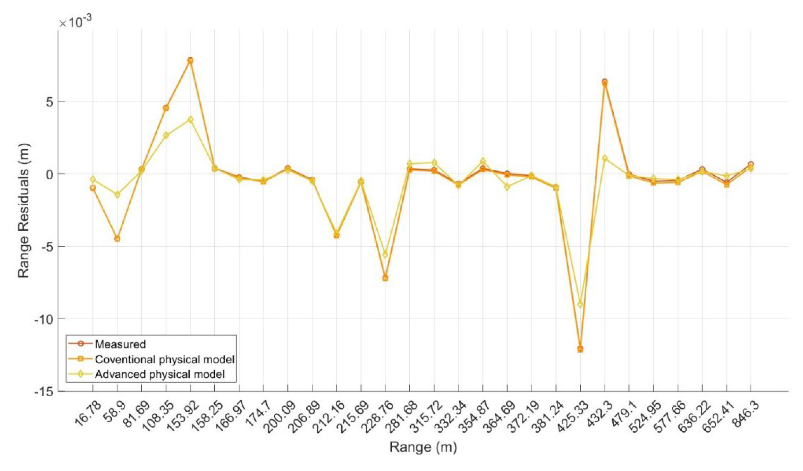
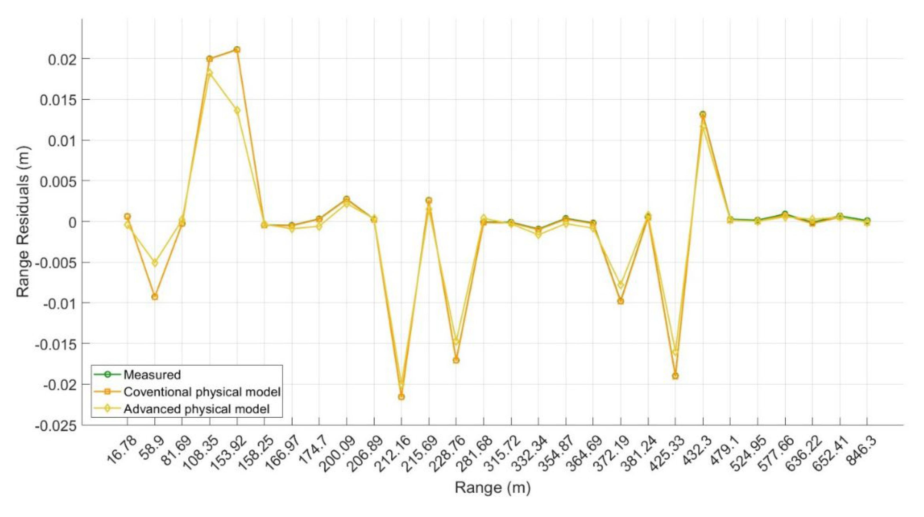
By integrating these vertical gradients along the propagation path, the advanced model provides corrected ranges and vertical angles that more accurately reflect real-world atmospheric conditions, bridging the gaps of the conventional approach. The results from the advanced model are then compared with those obtained from the conventional physical model (i.e., priori residuals represent the computed residuals after applying the conventional Ciddor refractive index model, while posteriori residuals correspond to the computed residuals after implementing the advanced Ciddor refractive index model (
Figure 8)).
Table 4 also compares the priori and posteriori uncertainties of the range observations in the range consistency method, expressed as root mean square error (RMSE) values. These highlight the improvements accomplished through the advanced model over the physical model.
Figure 8.
Comparison of range residuals in the range consistency method for the Leica ScanStation P50
( (Dataset 1: mine site)
9.
Figure 8.
Comparison of range residuals in the range consistency method for the Leica ScanStation P50
( (Dataset 1: mine site)
9.
Results indicate that the conventional physical refractive index model, based on average refractive indices at both endpoints of the range, results in consistency of the refractive index correction along the path, mostly account for the horizontal layer of the atmosphere, and is not able to significantly reduce range accuracy over the long baselines. As discussed earlier, this consistency remains important and cannot be overlooked due to the sensitivity of range observations to 3D spatial gradients of the refractive index (impacting the 3D spherical coordinates). However, a more advanced refractive index model, which accounts for the height profile within each vertically stratified atmospheric layer, less sensitive to the spatial gradients, leads to improved accuracy by approximately and 16% for the Leica ScanStation P50 and Maptek I-Site 8820, respectively. Note, both physical models provide identical RMSE values (priori uncertainties). This confirms the suitability of both physical models for TLS atmospheric correction.
Moreover, the moderate improvements in the range consistency method does not necessarily guarantee an identical level of improvements in 3D point coordinates accuracy. Due to the existence of large baselines and limited vertical viewing angles (i.e., the maximum vertical angle in mine site is approximately 14°), the sensitivity between vertical gradient of refractive index
and range refractive index
cannot be identified. Supporting this fact, the accuracy of the vertical angle is checked before and after applying the advanced model and realized to remain unchanged (
for the Leica ScanStation P50 and
Maptek I-Site 8820, with a slight sub-arcsecond improvement). However, the sensitivity between the two other horizontal gradients of refractive index
and range refractive index
for the points located within those limited fields-of-view is partially resolved (
and
accuracy improvement in X-coordinates and Y-coordinates, respectively (
Table 5)).
Generally, points observed at shallow vertical viewing angles exhibit reduced sensitivity to refraction effects. However, the absence of noticeable improvement in the Z-coordinates offers a stronger sensitivity between the vertical refractive index gradient
and the range refractive index
, which becomes more prominent at steeper vertical viewing angles (
Table 6). This behavior reflects the directional dependence of 3D point coordinate accuracy on the vertical gradients of the refractive index, depending on the vertical observed angle. Conventionally, the impact of atmospheric refraction on the X- and Y-coordinates is minimal for the points near the zenith, whereas Z-coordinates are more influenced by refraction changes (i.e.,
in Equation 1).
Results underscore that shorter baselines combined with larger vertical angles (dataset 2: dam site) are more influenced by atmospheric distortions than longer baselines integrated with smaller vertical angles (dataset 1: mine site). It is implied that the improved correction model not only enhances the accuracy of the vertical angle (
Table 6), but it also upgrades the range accuracy (due to diminished sensitivities (
Table 7)). Those mutual effects exceed the overall 3D point coordinate accuracy. Accordingly, the advanced physical model expands corrections along 3D point coordinates consistently, where higher percentage of improvement is expected for X- and Z-direction than Y-direction. It also acknowledges that the impact of the horizontal gradients of the refractive index on the overall accuracy of 3D point coordinates is minimum, in comparison with the maximum impact of the vertical gradient of the refractive index on 3D point coordinates.
In summary, the findings indicate a moderate level of improvement with the advanced physical refractive index model, Ciddor’s model (Equations 19 and 24), where 3D point coordinate accuracies were enhanced from the centimeter to the millimeter level for the Leica ScanStation P50, and predominantly in the Y-coordinate for the Maptek I-Site 8820. However, two major concerns remain and are worth further investigation: (1) the limited parameterization of
physical refractive index models for practical long-range terrestrial laser scanning (whether the Ciddor or the Closed Formula), and (2) the potential unreliability of 3D spatial gradients of atmospheric parameters, particularly vertical temperature gradients across stratified atmospheric layers, when applied to estimate refractive index gradients along the entire path in the
advanced physical refractive index model. These limitations have likely contributed to the insufficient improvements reported in
Table 7. To overcome these issues, hybrid physical–data-driven neural network models are proposed, supported by validated outcomes from physical modeling and cross-referenced with the control network.
5.3. Hybrid Refractive Index Model
The argued insights into physical refractive index modelling highlighted that a moderate reduction in the uncertainty of 3D point coordinates can be optimized, provided that the maximum possible precision for the estimation of the refractive index is assigned along the travelling path, with the least potential sensitivity between its spatial gradients.
Following this principle, a hybrid refractive index model is proposed. This approach enables the model to assign variable weights to the 3D spatial gradients of the refractive index, performing as a comprehensive solution to compensate for the inherent limitations of physical algorithms and to accurately evaluate atmospheric refraction along the line of sight. Consequently, the results aid in validating the field results obtained from advanced physical models and improving the overall 3D point coordinate accuracy (i.e., consistent millimeter level relative precision for the 3D point coordinates) through the nonlinear treatment of refractivity along the path across different scanning environments and using various scanners.
To support accurate prediction through this data-driven approach, it is recommended that remaining systematic errors be eliminated from both field datasets. However, they are expected to be insignificant in comparison to the priori standard deviation of observations – referring to
Table 1. Generally, the following steps must be taken:
Generate vectors of in-situ atmospheric recordings (e.g., air temperature, atmospheric pressure, and/or relative humidity and their spatial gradients) and intrinsic scanner characteristics (wavelength number, range, and angular accuracy) as the input data, to predict the refractive index as the output.
Implement the training of a neural network for the output function of refractive index and its spatial gradients.
Perform symbolic regression on the neural network outputs using physical interpretation of basis functions, such as Ciddor (Equations 13–19, 24, and 30) [
22,
23].
Derive closed-form symbolic expressions for refractive index, applicable to new atmospheric input conditions (optional) (For illustration, the MATLAB implementation of these steps is presented in the
Appendix D.).
Through symbolic expressions derived from the neural network, the increased precision for the estimation of refractive index and its gradients further reduces the sensitivity to spatial gradients of the refractive index. The posteriori uncertainties in range from the mine site dataset and vertical angle from the dam site dataset were reduced to
and
for the Leica ScanStation P50, and
and
for the Maptek I-Site 8820. Additionally, those consistently diminish the uncertainty of 3D point coordinates to reliable millimeter level (
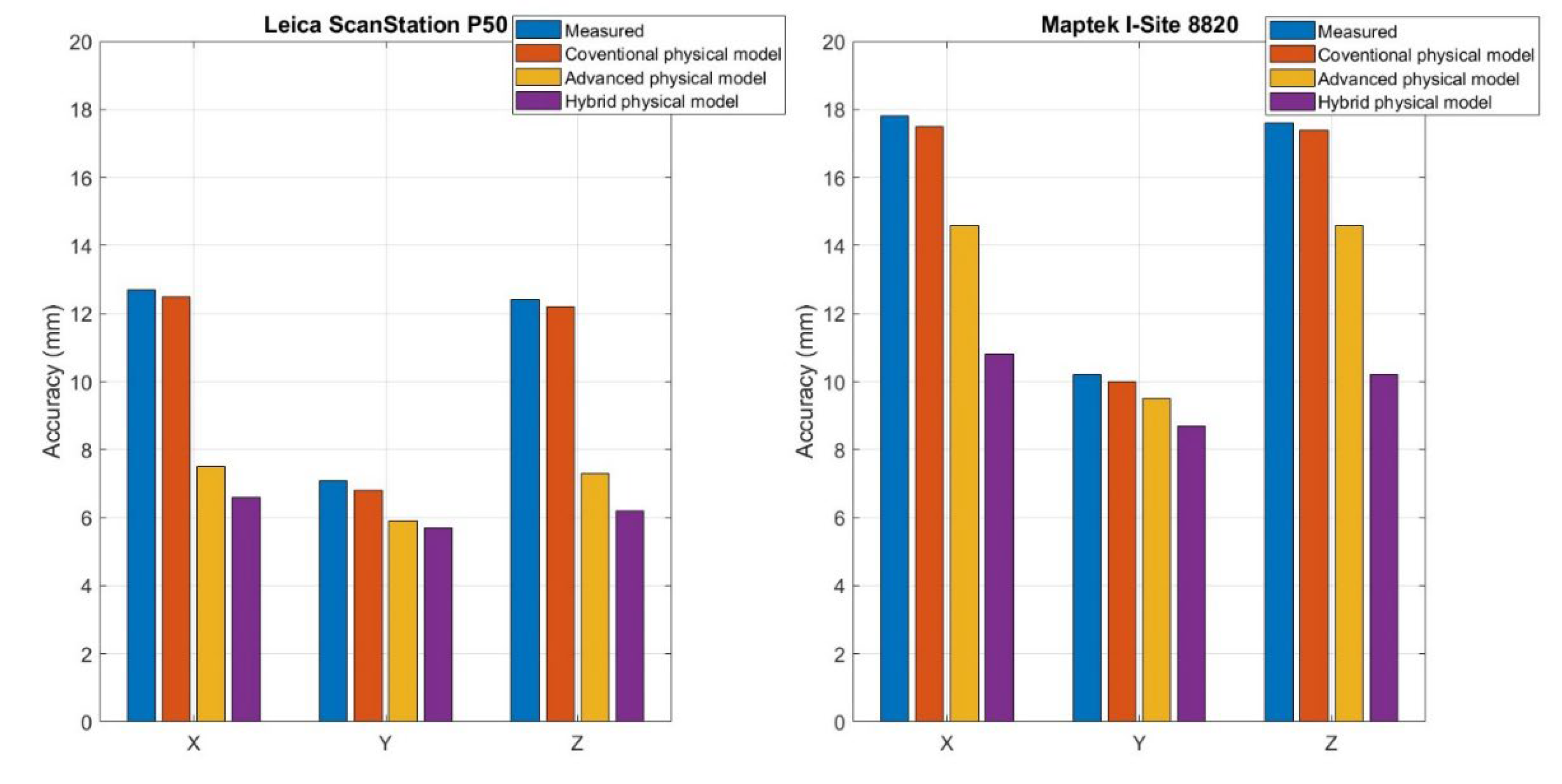
Figure 9).
Figure 9.
Accuracy comparison of 3D point coordinates under the three proposed methods.
Figure 9.
Accuracy comparison of 3D point coordinates under the three proposed methods.
Figure 9 illustrates the improvement in 3D point coordinate accuracy obtained through hybrid atmospheric correction models based on Ciddor developments - advancing refractive index estimation precision along the laser path and reducing uncertainty from the centimeter to the reliable millimeter level for the 3D point coordinates consistently. Worth emphasizing, both models, the advanced physical model and the hybrid model, consistently enhance 3D point coordinates accuracy, with particularly notable improvements in the X- and Z-coordinates. These results confirm the effectiveness of the proposed models in mitigating atmospheric errors in long-range terrestrial laser scanning compared to conventional physical refractive index modelling.
5.4. Discussions on Atmospheric Refraction Corrections
Previously, the impact of atmospheric refraction on the 3D point coordinates was investigated at two monitoring sites in terms of range and vertical angle refraction variations. Given
Table 5 and
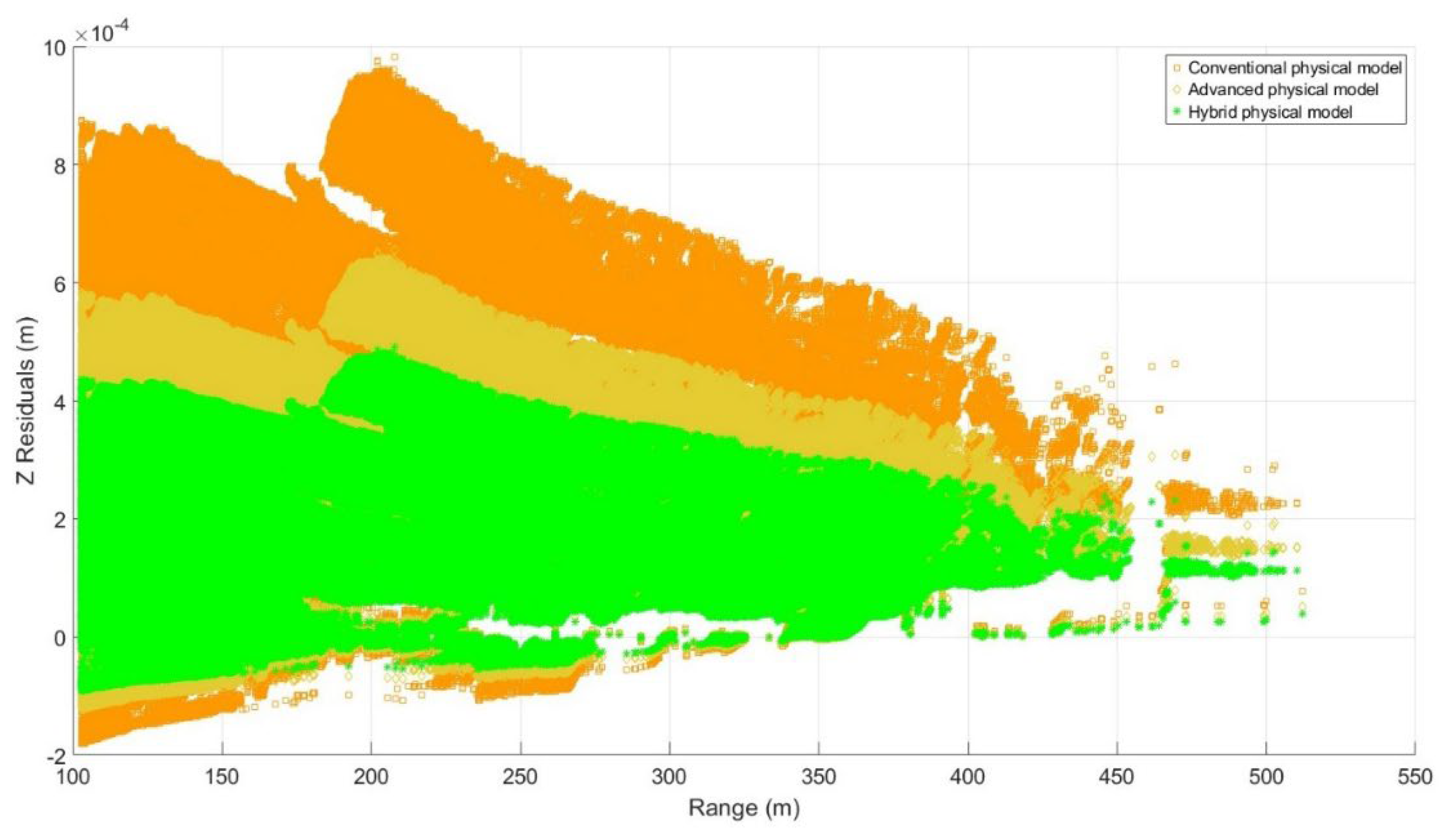
Table 7, it was shown that the improved atmospheric correction model primarily affects the Z-coordinates, with the maximum impact for the points close to the zenith, while the X- and Y-coordinates are minimally influenced for points close to the horizon and negligible changes close to the zenith. In the discussion section, the comparison of all observed points in each dataset with their corresponding ranges, vertical angles, and Z-residuals - obtained through three proposed refractive index models - is presented (
Figure 10 and
Figure 11). This further enables visualization of the behavior of the entire 3D point cloud after applying the atmospheric correction models for the dam site dataset, acquired by the Leica ScanStation P50 with extended simulated scanning ranges.
The results from the mine site demonstrate that the hybrid physical model substantially outperforms both the conventional and advanced physical models. As outlined before, the required corrections are at a sub-millimeter level for the observed ranges. Furthermore, the conventional model shows significant variations in atmospheric corrections, particularly at longer baselines than , while the advanced model reduces overall systematic bias for the entire range datasets consistently. Note, the larger variation in conventional methods is caused as the result of linear assumption of refractive index modelling which was addressed by weighted gradient indices in advanced and hybrid methods.
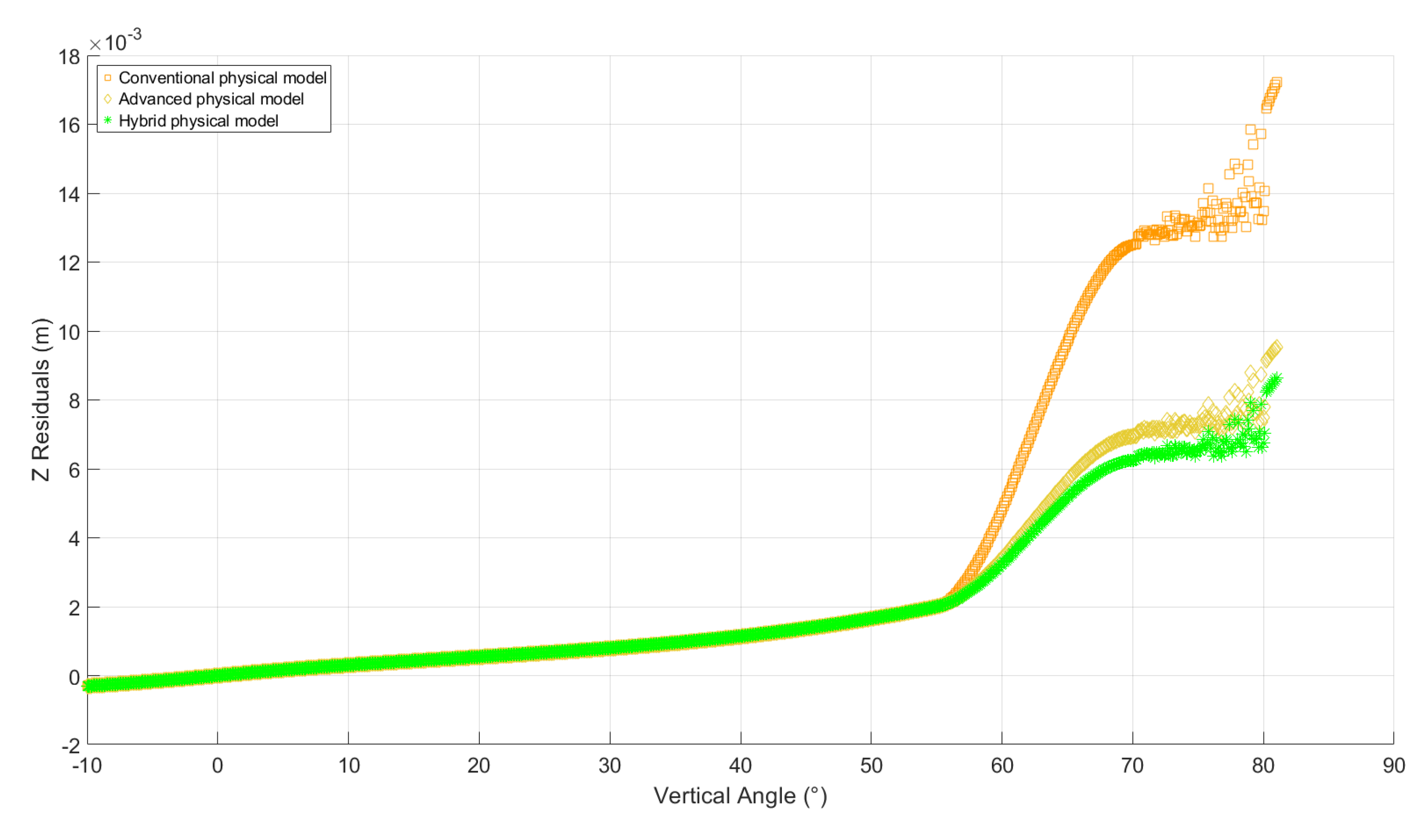
The analysis of the second dataset also reveals that the observations at larger vertical angles (particularly greater than
have a considerably higher impact than the observations at shallower vertical angles on the overall accuracy of the 3D point coordinates. This outcome arises due to the increasing sensitivity between range refraction and vertical gradient refraction, representing that the vertical gradient of refractive index dominates long-range TLS atmospheric error modelling, compared to the range refractive index in the mine site dataset. Importantly, the requirement to account for non-uniform atmospheric stratification and the anisotropic distribution of noise at larger vertical viewing angles is essential. Therefore, based on the successful results accomplished from advanced refractive index model, a combination of optimized weightings using the vertical gradient of refractive index into the advanced physical model provides a robust and intuitive solution to mitigate systematic atmospheric errors, allowing reliable millimeter- to sub-millimeter-level precision in 3D point cloud reconstruction for TLS-based deformation monitoring applications (
Figure 11).
Subsequently,
Figure 12 shows that, since atmospheric corrections are more significant at larger vertical angles, the high proportion of range corrections occurs from the Z-direction rather than the X- or Y-directions (i.e., the vertical angle observations are more sensitive to refractive index variations along the laser path). Consequently, this makes vertical angle corrections critical for ensuring the geometric accuracy of 3D point coordinates at long ranges (
Figure 13). To further illustrate the practical significance of atmospheric effects, comprehensive 3D point cloud simulations are conducted for the dam site dataset across three representative scanning ranges (
,
, and
(the maximum reported scanning range for the Leica ScanStation P50)), covering a vertical angle variation from
to
. The results of these simulations support the residual patterns identified in
Figure 10 and
Figure 11 (
Figure 13). At higher vertical angles (between
and
) and ranges greater than
, the atmospheric correction increases by more than a factor of two – from
to
. At the simulated maximum range of
, this correction reaches
.
6. Conclusions
The current research aimed to investigate the effect of atmospheric variations along the line of sight when long-range terrestrial laser scanning is required. The traveling laser beam through the atmosphere is predominantly affected by several optical phenomena. One of the most significant occurrences is the refraction of the optical path. Refraction causes deviations from the theoretical optical path and introduces variations in the intersection between the laser beam and the surface of the targets. This is identified as one of the systematic error sources in long-range scanning. To address the refractivity patterns along the optical path, the detailed mathematical developments of two physical refractive index models (the Ciddor and the Closed Formula) are elaborated here.
The physical model establishes the relationship between atmospheric conditions (air temperature, atmospheric pressure, and relative humidity) and the refractive index using the given wavelength. In the conventional approach, the average of refractive indices, based on the first and last terminals of the sightline, is obtained to address the linear condition of refractivity along the path. Furthermore, a higher precision on the order of
is recommended for the estimation of refractive index to ensure millimeter or sub-millimeter accuracy for the observations [
1]. For advancements of the physical models, 3D spatial gradients of the refractive index are developed in the current work, in relation to the nonlinear physical modelling where varying refractive indices along the path are demanded. These requirements are applied when the laser pulses experience the different medium (vertically stratified atmospheric layers).
In the field experiments for the atmospheric modelling, two long-range terrestrial laser scanners (Leica ScanStation P50 and Maptek I-Site 8820) were employed for quality testing under varying atmospheric conditions at two deformation monitoring sites: a mine site - enabling the long-range scanning over - and the dam site - providing the flexibility of steep vertical viewing angle close to zenith Both sites were controlled under a calibrated network arrangement, utilizing an on-site range consistency calibration method supported by GPS control points, along with field survey observations to verify vertical angle accuracy. During each scanning setup, the atmospheric conditions of air with respect to individual scanner station (in-situ atmospheric recordings attached to each station) were tracked across the entire sites.
The recognized ranges from the mine site dataset were evaluated for network reliability, and after maximizing the precision of refractive index estimation through advanced approach of physical refractive index model, the improvements of
for the Leica ScanStation P50 and 16% the Maptek I-Site 8820 in range accuracy were observed. Since a number of points were located at the shallow vertical angle in the mine site, the sensitivity to 3D spatial gradients of the refractive index – specifically, vertical gradient of refractive index across stratified atmospheric layers – was not detected, and this led to limited improvement in 3D point coordinate uncertainties. The dam site dataset demonstrates mitigation strategies for this sensitivity, particularly for points located at higher elevations (with vertical viewing angles larger than 60°). With the advanced physical model, improvements occurred not only in the a posteriori accuracy of the vertical gradient of the refractive index (44% (from
to
) for the Leica ScanStation P50 and
(from
to 19”) for the Maptek I-Site 8820), but also in the accuracies of the 3D point coordinates (reliable centimeter- to millimeter-level accuracy). The reason is that the points, located on approximately the same horizontal plane as the scanner station, are more uniformly affected by atmospheric corrections (dataset 1: mine site), while the points, located at different horizontal planes, require larger X- and Z-coordinate corrections (dataset 2: dam site). The hybrid model, referencing back to the advanced physical refractive index model, is advised to achieve higher millimeter-level relative precision in 3D point coordinates consistently. Millimeter-level accuracy is ultimately attained by reducing the range and vertical angle uncertainties to
and
for the Leica ScanStation P50, and
and
for the Maptek I-Site 8820 (
Table 6). The advantage of the proposed approaches - the advanced and hybrid physical models - is their ability to represent real-world refractivity conditions along the laser path by maximizing the precision of refractive index estimation and minimizing sensitivity to spatial gradients, achieved through a stochastic weighting of the vertical refractive index gradient within different atmospheric layers.
For future work, several pathways exist toward achieving millimeter- or sub-millimeter-level accuracy in the field calibration of long-range terrestrial laser scanning. First, additional optical effects of the laser line, such as scattering and reflection, play an integral role in determining robust radiometric and spatial calibration results. Second, the algorithmic steps presented here for the physical refractive index model are recommended to be further modified based on more accurate in-situ atmospheric observations (e.g., temperature accuracy better than ). This is particularly suggested for highly sensitive and high-risk deformation projects. Preferably, attached thermometer arrangements should enable recording of the epoch-wise atmospheric conditions of the laser. Alternatively, for advanced physical refractive index modelling, it is strongly recommended to create a temperature heat map sensitive to height profiles, as the dominating factor, to better indicate temperature variations across the monitoring test sites. Third, the use of an appropriate stochastic model for 3D spherical observations is highly advised for comprehensive system calibration of the 3D point cloud, addressing geometric error models. Finally, the relevant atmospheric correction factors should be ideally applied within the instrument, enhanced by a robust atmospheric measurement technique along the entire path which can be supported by the manufacturing principal assembly.
Figure 1.
Different techniques for range measurement (from left to right: time of flight (TOF), phase-based, and waveform digitizer (WFD)) [
5].
Figure 1.
Different techniques for range measurement (from left to right: time of flight (TOF), phase-based, and waveform digitizer (WFD)) [
5].
Figure 2.
Different techniques for angle measurements (from left to right: camera, hybrid and panoramic scanner) [
8].
Figure 2.
Different techniques for angle measurements (from left to right: camera, hybrid and panoramic scanner) [
8].
Figure 3.
Geodetic refraction over the line of the sight [
9].
Figure 3.
Geodetic refraction over the line of the sight [
9].
Figure 4.
(Left to right) vertical refraction on
plane and horizontal refraction on
plane (convex condition) [
10,
28].
Figure 4.
(Left to right) vertical refraction on
plane and horizontal refraction on
plane (convex condition) [
10,
28].
Figure 5.
Mine site (Dataset 1) and dam site (Dataset 2).
Figure 5.
Mine site (Dataset 1) and dam site (Dataset 2).
Figure 6.
(from left to right) Leica ScanStation P50, and Maptek I-Site 8820.
Figure 6.
(from left to right) Leica ScanStation P50, and Maptek I-Site 8820.
Figure 7.
Temperature recordings and their variations.
Figure 7.
Temperature recordings and their variations.
Figure 8.
Comprehensive calibration methodologies.
Figure 8.
Comprehensive calibration methodologies.
Figure 9.
Control ranges, height differences, and the residuals in the range consistency method (Dataset 1: mine site).
Figure 9.
Control ranges, height differences, and the residuals in the range consistency method (Dataset 1: mine site).
Figure 10.
Distribution of Z-residuals () with respect to range observations (), with standard deviation of for both X- and Y-coordinates resulting from the implementation of hybrid model (Dataset 1: mine site).
Figure 10.
Distribution of Z-residuals () with respect to range observations (), with standard deviation of for both X- and Y-coordinates resulting from the implementation of hybrid model (Dataset 1: mine site).
Figure 11.
Distribution of Z-residuals () with respect to vertical angle observations (), with standard deviations of and for the X- and Y-coordinates resulting from the implementation of hybrid model, respectively (Dataset 2: dam site).
Figure 11.
Distribution of Z-residuals () with respect to vertical angle observations (), with standard deviations of and for the X- and Y-coordinates resulting from the implementation of hybrid model, respectively (Dataset 2: dam site).
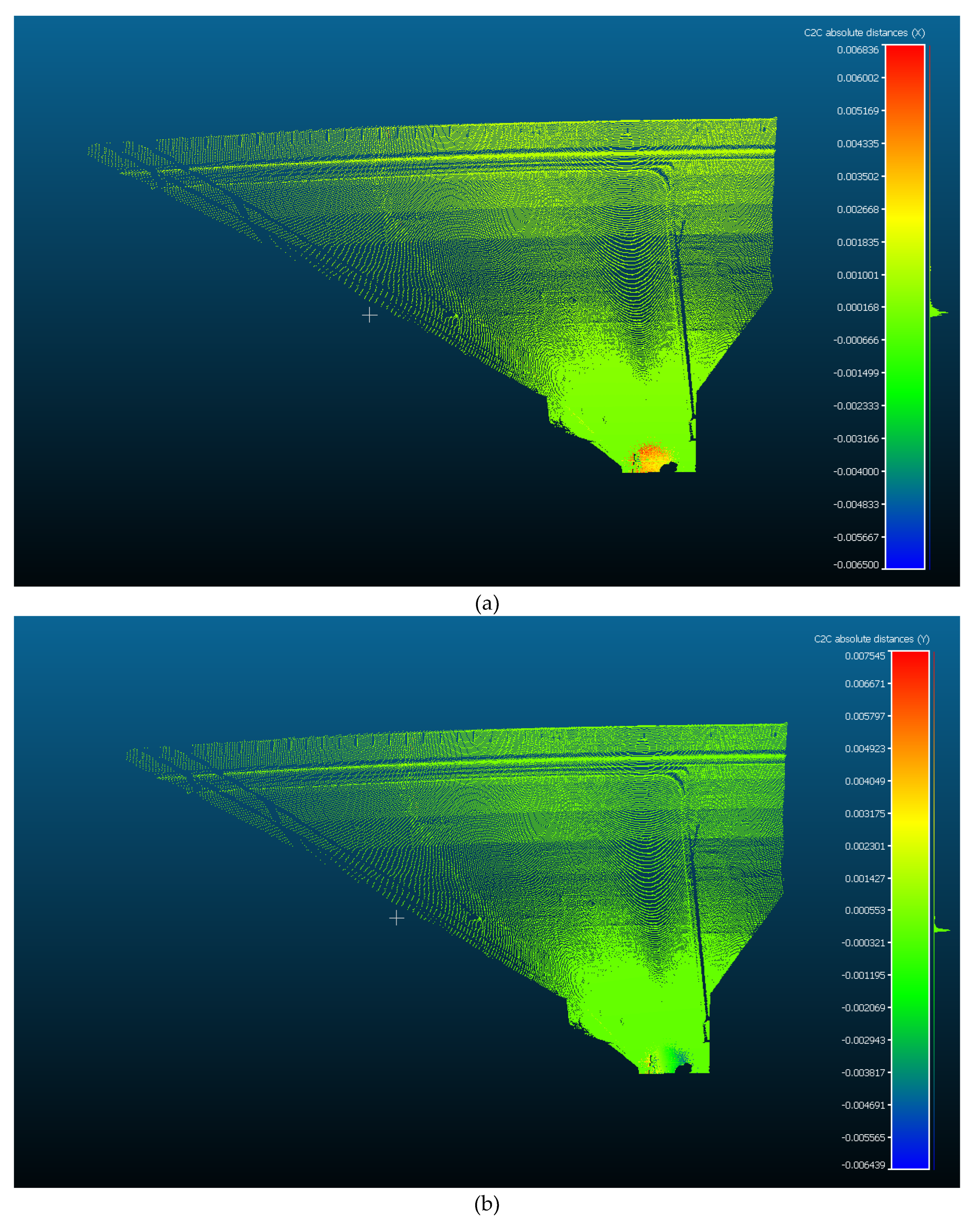
Figure 12.
Distribution of (a) X-corrections, (b) Y-corrections, (c) Z-corrections, and (d) range corrections resulting from the implementation of hybrid model (Dataset 2: real dam site).
Figure 12.
Distribution of (a) X-corrections, (b) Y-corrections, (c) Z-corrections, and (d) range corrections resulting from the implementation of hybrid model (Dataset 2: real dam site).
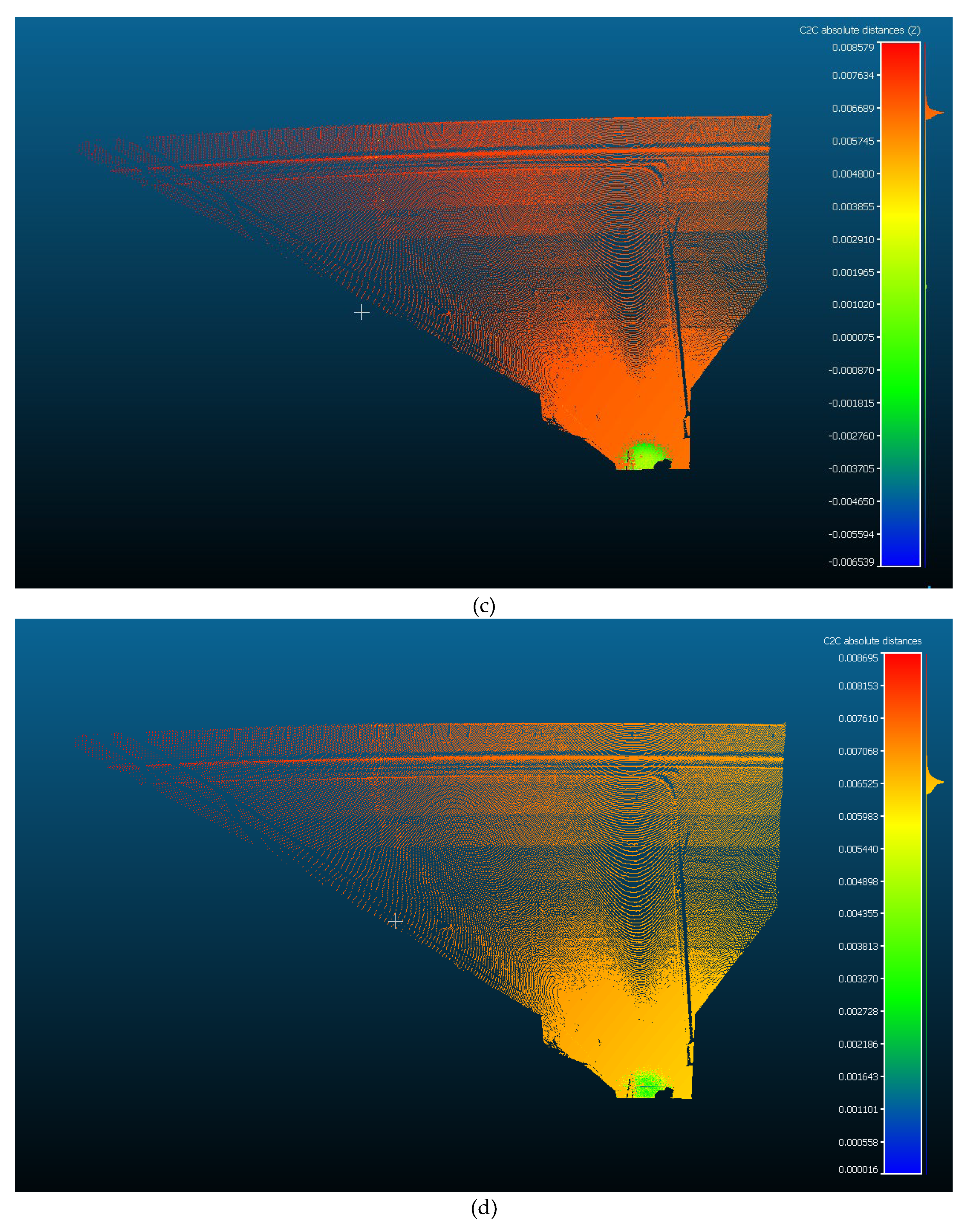
Figure 13.
Distribution of range corrections resulting from the implementation of the hybrid model (Dataset 2: simulated dam site at scanning ranges of (a) , (b) , and (c) ).
Figure 13.
Distribution of range corrections resulting from the implementation of the hybrid model (Dataset 2: simulated dam site at scanning ranges of (a) , (b) , and (c) ).
Table 1.
Proposed methods for refractive index modelling in TLS-based applications.
Table 1.
Proposed methods for refractive index modelling in TLS-based applications.
| Methods |
Refractive index models |
Approaches |
| Conventional physical model (Section 5.1) |
Ciddor and Closed Formula |
Average of refractive indices from both terminals (linear) |
Advanced physical model
(Section 5.2) |
Developed Ciddor |
Incorporating varying vertical refractive indices (non-linear) |
Hybrid physical model
(Section 5.3) |
Developed Ciddor and Neural Network |
Combination of the results from advanced model with a neural network (data-driven) |
Table 2.
Scanner specifications and undertaken scanning characteristics.
Table 2.
Scanner specifications and undertaken scanning characteristics.
| Specifications (scanner and scanning) |
Leica
ScanStation P504
|
Maptek
I-Site 88205
|
| Accuracy |
Range |
(over full range (over full range ) |
|
| Angle |
|
|
| Maximum possible range of scanning |
|
|
| Wavelength |
|
|
| Measurement techniques |
Range |
TOF |
TOF |
| Angle |
Panoramic |
Hybrid |
| Field-of-view |
Vertical |
|
|
| Horizontal |
|
|
| Instrumental resolution |
at |
fine resolution |
| Time per scan |
minutes |
minutes |
Table 3.
Vertical temperature gradient
for each vertically stratified atmospheric layer [
29].
Table 3.
Vertical temperature gradient
for each vertically stratified atmospheric layer [
29].
| Atmospheric layers |
|
| Lowest |
Variant (between and |
| Intermediate |
|
| Highest |
Variant (between and |
Table 4.
Priori and posteriori range accuracy in the range consistency method (Dataset 1: mine site).
Table 4.
Priori and posteriori range accuracy in the range consistency method (Dataset 1: mine site).
|
|---|
| TLSs |
Leica ScanStation P50 |
Maptek I-Site 8820 |
| Measured |
3.6 |
9.1 |
| Priori |
Ciddor |
3.6 |
9.1 |
| Closed Formula |
3.6 |
9.1 |
| Posteriori * |
2.4 |
7.6 |
| Improvement |
34% |
16% |
Table 5.
Priori and posteriori accuracy of 3D point coordinates (Dataset 1: mine site).
Table 5.
Priori and posteriori accuracy of 3D point coordinates (Dataset 1: mine site).
| TLSs |
3D point coordinates |
|
| Priori |
Posteriori |
Leica
ScanStation P50
|
|
10.5 |
10.3 |
|
7.8 |
7.3 |
|
27.8 |
27.8 |
Maptek
I-Site 8820
|
|
16.4 |
16.1 |
|
13.5 |
12.7 |
|
37.1 |
37.1 |
Table 6.
Priori and posteriori vertical angle accuracy (Dataset 2: dam site).
Table 6.
Priori and posteriori vertical angle accuracy (Dataset 2: dam site).
|
|---|
| TLSs |
Leica ScanStation P50 |
Maptek I-Site 8820 |
| Priori |
18” |
24” |
| Posteriori |
10” |
19” |
| Improvement |
44% |
20% |
Table 7.
Priori and posteriori accuracy of 3D point coordinates (Dataset 2: dam site).
Table 7.
Priori and posteriori accuracy of 3D point coordinates (Dataset 2: dam site).
| TLSs |
3D point coordinates |
Uncertainty
|
Improvement |
| Priori |
Posteriori |
Leica
ScanStation P50
|
|
12.7 |
7.5 |
41% |
|
7.1 |
5.9 |
17% |
|
12.4 |
7.3 |
41% |
Maptek
I-Site 8820
|
|
17.8 |
14.6 |
18% |
|
10.2 |
9.5 |
7% |
|
17.6 |
14.6 |
17% |