An Interpretation of Gardner’s Equations

Joseph Higginbotham

doi:10.20944/preprints202509.0328.v1

Submitted:

02 September 2025

Posted:

03 September 2025

You are already at the latest version

Abstract

Gardner’s equation that relates porous rock density to the P-wave velocity and is used to analyze seismic amplitude information. The exponential form of the equation is convenient for this use. However the equation was found by fitting data from basins from all over the world. Here a simple basin compaction model is used to show that the form of Gardner’s equation is due primarily to basin compaction which happens to match with variation of rock density and P-wave velocity for sandstone but often fails for shale. An alternative equation is evaluated and shown to be a better choice for single basin use. It is also shown that when Gassmann’s equations are combined with Nur’s critical porosity model the resulting equations relating the shear wave velocity to the P-wave velocity and the density to the p-wave velocity can be written in a way that does not involved the pore fluid bulk modulus. This may explain why so many mono-mineral rocks display a hyperbolic relation between the shear wave velocity and the P-wave velocity with constants independent of porosity for a given pore fluid.

Keywords:

Gardner's Equation

;

Gassman-Nur

;

critical porosity

Subject:

Environmental and Earth Sciences - Geophysics and Geology

Introduction

Gardner’s equation that relates porous rock density to the P-wave velocity has been revered as, “One of the most important empirical [relations] in seismic prospecting ….” [1]. A web search on “Gardner’s Equation” finds 371,000 results some of which are recent technical articles mentioning the equation in the title. The equation plays an important role in seismic amplitude analysis, involving the fluid factor attribute for example, and is important to velocity associated pore pressure prediction. Its accuracy is thereby connected to economics associated with reservoir development and production and aquifer evaluation. It is understood that this equation is influenced by compaction. Here evidence is presented to show how the equation depends on compaction and that it may depend strongly on the compaction characteristics of a basin in some cases. This is done using the Gassmann-Nur model for porous rock, discussed later under heading Quartz-Shale Composite Models, together with a basin compaction model following Aplin [2]. Finally evidence is presented in support of an alternative equation relating bulk density to P-wave velocity. Justification is provided for the use, with low permeability rocks, of Gassmann’s equations combined with Nur’s critical porosity model to derive the subject relations. This justification requires replacing the fluid bulk modulus with other physical quantities associated with the rock.

Gardner’s equation [3] is often used to roughly estimate rock density from the rock P-wave velocity

V_{p}

. The equation has the convenient form of

ρ = ρ_{0} V_{p}^{1 / 4}, ρ_{o} = 1741 {(k m / s)}^{\frac{- 1}{4}}

(1)

Figure 1 shows Gardner’s relation that essentially separates the sandstones, red squares, from shales, green squares digitized from Castagna et al. (1993, Fig. 9). The Violet (kaolinite) and Cyan (smectite) curves are from Mondol et al. [4].

Method

In Figure 2 is shown data, red circles, from two wells in the same basin which curve in the wrong direction to be following Gardner’s relation. In addition the black circles are a fit of the equation

ρ = \frac{C_{ρ}}{1 - {(\frac{s V_{p}}{V_{b}})}^{2}}, with V_{b} = 1500 m / s

(2)

Here the constant

V_{b}

is used to scale

V_{p}

so that

s

is a unitless constant. Equation (2), and a hyperbolic relation between

V_{p}

and

V_{s}

, are the result of combining Gassmann’s equations [5] with Nur’s critical porosity model [6,7] – called Gassmann-Nur model here.

C_{ρ}

and

s

are constant for a given mineral. Formulas for these constants that depend only on the mineral grain bulk modulus, shear modulus, fluid bulk modulus and rock critical porosity are provided by Higginbotham et al. [7].

One important difference between the data in Figure 1 and Figure 2 is that the data plotted in Figure 1 is from a variety of basins from all over the world while the data in Figure 2 is from a single basin. The goal here is to provide evidence that the major structure of Gardner’s equation is due to the compaction characteristics of the basin from which each data point was taken and that, for a given basin, equation (2) is more appropriate.

Sandstone

The curves in Figure 3 were computed from published elastic constants for quartz using a fluid density of 1.02 and a fluid bulk modulus of 2.5 GPa. The model provides an excellent fit to the data. Since both the bulk modulus

K

and the shear modulus

μ

are involved in computing the P-wave velocity

V_{p}

it is reasonable to assume that the Gassmann-Nur model works well for clean silicon sandstone even without similar data for the S-wave velocity

V_{s}

. So equation (2) should work well to describe clean silicon sandstone.

Shale

Applying Gassmann’s equations to Shale rocks presents a problem because shale is porous but not very permeable. Gassmann’s equations apply at low frequency where, quoting Mavko et al. [9], “there is sufficient time for the pore fluid to flow and eliminate wave-induced pore -pressure gradients ….”

The fluid density is not likely to change significantly due to pore pressure so the problem with Gassmann’s equations must be associated with variations in the pore fluid bulk modulus due to induced pore-pressure gradients.

Avoiding $K_{f}$

Equation (A5) of Higginbotham et al. [7] can be solved for the pore fluid bulk modulus

K_{f}

to get a definition of an effective fluid bulk modulus,

K_{f - e f f e c t i v e} = K_{m} d / (1 + d), d = ϕ_{c}' - ϕ_{c}

(3)

in terms of the mineral grain bulk modulus

K_{m}

the critical porosity of Nur,

ϕ_{c}

, and the quantity

ϕ_{c}'

. With reference to Figure 4, the quantity

ϕ_{c}

corresponds to the negative reciprocal of the slope of the rock shear modulus divided by the mineral grain shear modulus when plotted against porosity. The quantity

ϕ_{c}'

corresponds to the negative reciprocal of the slope of the rock bulk modulus divided by the mineral grain bulk modulus when plotted against porosity. The equation applies only when the porosity is less than Nur’s critical porosity, in other words for any load bearing rock matrix. The quantities defining

d

in equations (3) are well defined measurable physical quantities. They can be read directly from a graph such as the one in Figure 4.

K_{m}

is know if the mineral making up the rock matrix is known. These two physically measurable quantities replace

K_{f}

in all the equations. Although

K_{f}

ceases to exist in the equations it can be used, along with

K_{m}

, to approximate

d

,

d \approx K_{f} / (K_{m} - K_{f})

(4)

This will be a good approximation for permeable rocks. It also turns out to be a good approximation for the smectite data of Mondol et al. [4] but not quite as accurate for representing

d

for the kaolinite data and fails to predict

d

for dry rocks for kaolinite. In that case

d

must be measured from a graph as in Figure 4.

Claim: When Nur’s critical porosity model is combined with Gassmann’s equations and equation (3) is used to eliminate the explicit appearance of the fluid bulk modulus in the equations, the effects associated with fluid properties vanish to first order. Here this will be called the modified Gassmann-Nur model.

As a result this modified Gassmann-Nur model applies to a wide variety of rocks and at high frequency. The “catch” is that the physical quantity

d

is involved in the new equations and the direct connection to fluid bulk modulus is lost.

Of course this does not prevent the use of Gassmann’s equations alone for such things as fluid substitution for example. It does significantly extend the usefulness of Gassmann’s equations when combined with Nur’s model. In particular it justifies the form of equation (2) whenever

ϕ_{c}

and

ϕ_{c}'

are constant, or approximately constant for a wide variety of rocks and for shale rocks made up of Smectite or Kaolinite in particular - see Figure 4 (for further evidence see Higginbotham [12] (supplemental material slides 14-18).

Quartz-Shale Composite Models

A method of modeling overburden compacted composite rocks made up of quartz and shale is provided by Higginbotham [12] (Appendix II). This method, as used here, finds density and velocity by using Nur’s critical porosity model combined with the equation provided by Aplin [2], relating porosity to vertical effective stress through a compaction coefficient

β

. This information is then tested against equation (2) above which combines Nur’s model with Gassmann’s equations. The question is, “Will this modeling combining Nur’s model with Aplin’s relation agree with equation (2) combining Nur’s model with Gassmann’s equations? If so, what does this indicate about Gardner’s equation?”

Results

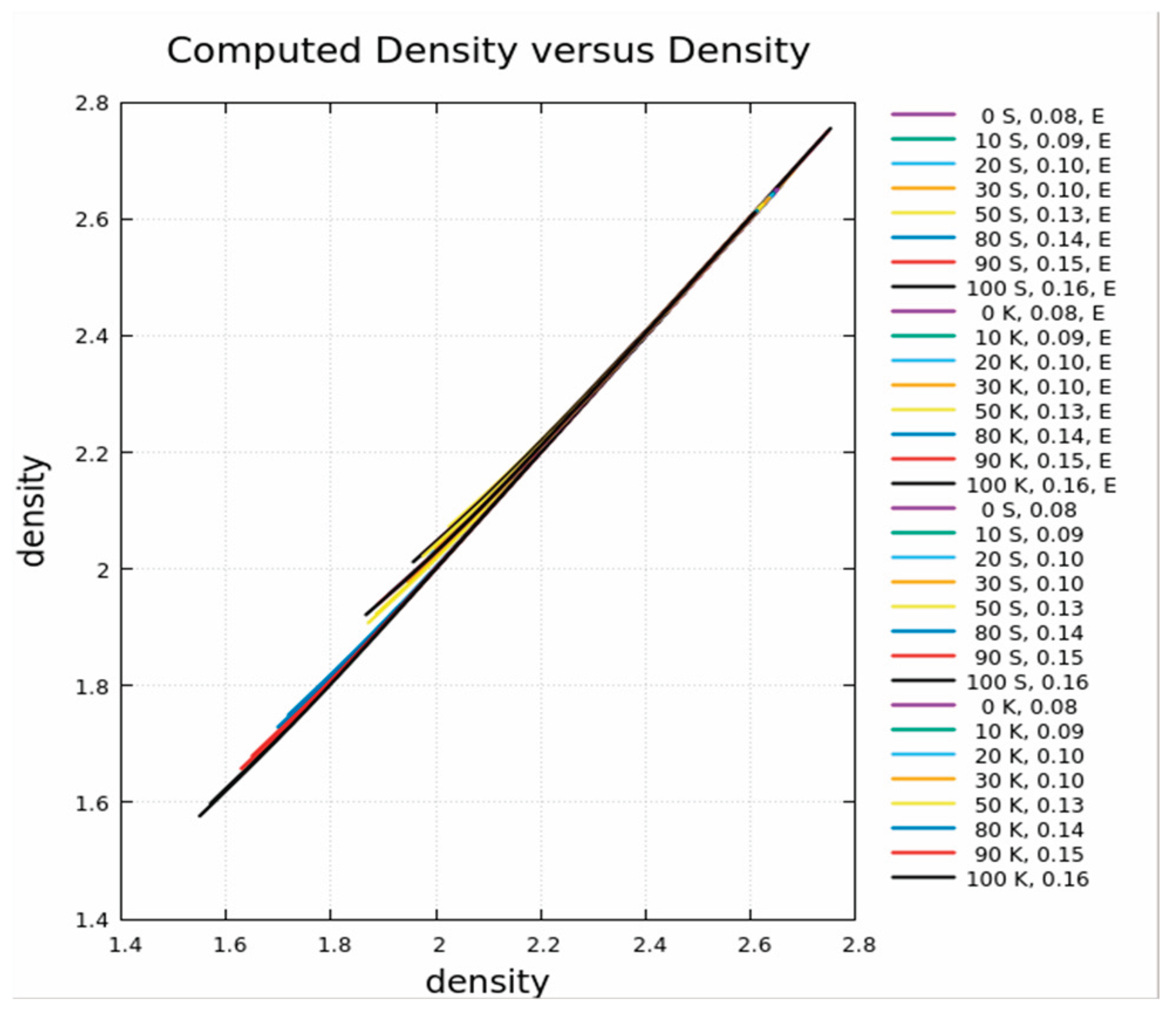
Results of modeling are shown in Figure 5 with the data points for sandstone and shale plotted in the foreground. These curves for smectite-quartz composite rocks and kaolinite-quartz composite rocks account for all of the data points that are roughly fit by Gardner's relation with the high percentage sand cases above Gardner’s relation and the low percentage sand below – also in agreement with Gardner. The modeled density matched well with the density computed using equation (2) for models represented in Figure 5, see Figure 6. Note that Figure 6 includes cases for both the effective fluid bulk modulus and for the actual fluid bulk modulus. The deviation for kaolinite-quartz composite rock was roughly twice as large as for smectite-quartz composite rock but both are small.

Conclusions

Modified Gassmann-Nur Model

An effective fluid bulk modulus replaced the actual fluid bulk modulus to implement the modified Gassman-Nur model which has no explicit dependence on the fluid bulk modulus. Combining Gassmann’s equations with Nur’s critical porosity model leads to equation (2), as well as a hyperbolic equation relating

V_{p}

to

V_{s}

, both involving constants that are independent of porosity for a given mineral and pore fluid. These two equations and the formulas representing the associated constants comprise the Modified Gassmann-Nur model. Here attention has been focused on equation (2) in an effort to better understand Gardner’s equation. The absence of the fluid bulk modulus provides justification for the use of modified Gassmann-Nur model at high frequency for low permeability rocks and also explains the fact that many rocks satisfy the hyperbolic relation between the P-wave velocity and S-wave velocity (Higginbotham [12], supplemental material, slides 3-18, and Higginbotham et al., [13]). The overwhelming evidence indicates that this is common rather than the exception. Exceptions do exist and probably correspond to cases where the quantity

d

deviates significantly from a constant value.

Gardner’s Equation

Gardner’s equation is shown to be representative of the trend associated with how density changes with velocity as basins having different compaction coefficients are compared. Figure 5 shows that the slope of Gardner’s equation and equation (2) are similar for high percentage sandstone rocks. So sandstone reservoirs can be represented by Gardner’s equation as well as by equation (2). However shale reservoirs do not match well with the slope of Gardner’s equation. For a specific reservoir, equation (2) is the more appropriate relation.

Funding

This work was funded by Z-Terra Inc., Houston, TX

Conflicts of interest

The author declares no conflict of interest.

Appendix A Path to Gassman’s Equations

A quick path to Gassmann’s equations

Note: I found some hints in text on the internet, source lost to mind now, that led me to this path to Gassmann’s equation for Bulk Modulus. So the logic is mine but the inspiration is not.

There are more rigorous derivations of Gassmann’s equations [14] that make the point that Gassmann does not assume that the shear modulus is constant (i.e., mechanically independent of the presences of the saturating fluid) which is an assumption made here near the end of this path.

Consider a uniform porous cube of mono-mineral rock that is permeable having volume

V

.

Suppose that the load bearing rock frame is fraction

β

of the volume of the porous rock with pores filled with fluid. The remaining volume fraction consists of the fluid that fills the rock pores together with any loose mineral grains within the pores more or less suspended in the fluid – at least not contributing to the rigidity of the rock frame.

Now suppose that the rock is uniformly compressed creating strain

Δ V / V

. Since the compression is uniform the fractional change in volume of the load bearing rock matrix portion and the fractional change in the volume of the fluid and suspended mineral particle portion will be the same and equal to the fractional change in volume of the full rock volume, or

{(\frac{Δ V}{V})}_{f r a m e} = {(\frac{Δ V}{V})}_{f l u i d s u s p e n s i o n} = \frac{Δ V}{V}

(1)

But the rock frame and the pore fluid will resist being compressed. The compression stress (pressure) on the rock

P

will be the sum of the stress on the load bearing rock matrix portion

P_{m}

and the stress on the fluid suspension portion

P_{s}

, weighted by the fractional amount of each

P = P_{m} + P_{s}

(2)

K_{w} \frac{Δ V}{V} = β K_{m} \frac{Δ V}{V} + (1 - β) K_{s} \frac{Δ V}{V}

(3)

with

K_{w}

representing the bulk modulus of the wet (fluid saturated) rock,

K_{m}

representing the bulk modulus of the mineral grains forming the rock frame, and with , the effective bulk modulus of the fluid suspension, to be determined .

Then

K_{w} = β K_{m} + (1 - β) K_{s}

(4)

Now consider the fluid suspension portion of the rock. This is the portion composed of the fluid under pressure

P_{f}

and loose mineral grains within this fluid. The loose mineral grains will also experience the same pressure as the pore fluid. The total change in volume for this portion of the rock will be the sum of the change in volume of the fluid and the loose mineral grains,

\frac{P_{f}}{K_{s}} = {(\frac{Δ V}{V})}_{f l u i d s u s p e n s i o n} = \frac{Δ V_{f l u i d} + Δ V_{l o o s e g r a i n s}}{V_{f l u i d s u s p e n s i o n}} = \frac{Δ V_{f l u i d}}{V_{f l u i d s u s p e n s i o n}} + \frac{Δ V_{l o o s e g r a i n s}}{V_{f l u i d s u s p e n s i o n}}

(5)

V_{f l u i d s u s p e n s i o n} = (1 - β) V

(6)

V_{f l u i d} = ϕ V

(7)

V_{l o o s e g r a i n s} = V - V_{f l u i d} - V_{f r a m e} = V (1 - ϕ - β)

(8)

Using equation (6) in equation (5) leads to,

\frac{P_{f}}{K_{s}} = \frac{Δ V_{f l u i d}}{(1 - β) V} + \frac{Δ V_{l o o s e g r a i n s}}{(1 - β) V}

(9)

Now use equations (7) and (8) to replace

V

in equation (9) to get,

\frac{P_{f}}{K_{s}} = \frac{Δ V_{f l u i d}}{(1 - β) \frac{V_{f l u i d}}{ϕ}} + \frac{Δ V_{l o o s e g r a i n s}}{(1 - β) \frac{V_{l o o s e g r a i n s}}{1 - ϕ - β}}

(10)

Then using

P_{f} / K_{f} = Δ V_{f l u i d} / V_{f l u i d}

and, recalling that the loose mineral grains experience the same pressure as the pore fluid,

P_{f} / K_{m} = Δ V_{l o o s e g r a i n s} / V_{l o o s e g r a i n s}

gives,

\frac{P_{f}}{K_{s}} = \frac{P_{f} ϕ}{(1 - β) K_{f}} + \frac{P_{f} (1 - ϕ - β)}{(1 - β) K_{m}}

or

\frac{1}{K_{s}} = \frac{1 ϕ}{(1 - β) K_{f}} + \frac{1 (1 - ϕ - β)}{(1 - β) K_{m}}

(11)

Now returning to equation (4) notice that when the fluid is drained from the pores then the fluid suspension portion, represented by the term involving

K_{s}

vanishes and

K_{w}

becomes

K_{d}

the dry or drained rock bulk modulus,

K_{d} = β K_{m}

(12)

Now solving equation (12) for

β

and equation (11) for

K_{s}

and using these in equation (4) leads to

Gassmann’s equation in the form,

K_{w} = K_{d} + \frac{{(1 - \frac{K_{d}}{K_{m}})}^{2}}{\frac{ϕ}{K_{f}} + \frac{1 - ϕ}{K_{m}} - \frac{K_{d}}{K_{m}^{2}}}

(13)

The other equation by Gassmann is,

μ_{w} = μ_{d}

(14)

which says that the fluid saturated rock shear modulus is equal to the dry (or drained) rock shear modulus. If we assume that the fluid filling the rock pores does not support shear stress then this result appears to be obvious since a shear stress on the porous rock does not change the rock volume to first order.

References

Castagna, J.P., Batzle, M.L., & Kan, T.K. (1993). Rock physics – the link between rock properties and AVO response. In J.P. Castagna & M.M. Backus (Eds.), Offset-dependent reflectivity: theory and practice of AVO Analysis. SEG, 135-171.
Aplin, A.C.; Yang, Y.; Hansen, S. Assessment of β the compression coefficient of mudstones and its relationship with detailed lithology. 2000, 12, 955–963. [Google Scholar] [CrossRef]
Gardner, G.H.F.; Gardner, L.W.; Gregory, A.R. Formation velocity and density-the diagnostic basics for stratigraphic traps. Geophysics 1974, 39, 770–780. [Google Scholar] [CrossRef]
Mondol, N.H.; Jahren, J.; Bjørlykke, K.; Brevik, I. Elastic properties of clay minerals. Lead. Edge 2008, 27, 758–770. [Google Scholar] [CrossRef]
Gassmann, F. ELASTIC WAVES THROUGH A PACKING OF SPHERES. Geophysics 1951, 16, 673–685. [Google Scholar] [CrossRef]
Mavko, G.; Mukerji, T. Comparison of the Krief and critical porosity models for prediction of porosity and VP/VS. Geophysics 1998, 63, 925–927. [Google Scholar] [CrossRef]
Higginbotham, J.H.; Macesanu, C.; Brown, M.P.; Ramirez, O.; Joanne, C. An alternative amplitude analysis theory. SEG Technical Program Expanded Abstracts 2012. LOCATION OF CONFERENCE, COUNTRYDATE OF CONFERENCE; pp. 1–5.
Nur, A., Mavko, G., Dvorkin, J., & Galmundi, D. (1998). Critical porosity: A key to relating physical properties to porosity in rocks. The Leading Edge, 357.
Mavko, G., Mukerji, T., & Dvorkin, J. (2009). The Rock Physics Handbook (2nd ed.). Cambridge University Press, New York.
Vernik, L.; Kachanov, M. Modeling elastic properties of siliciclastic rocks. Geophysics 2010, 75, E171–E182. [Google Scholar] [CrossRef]
Vernik, L.; Kachanov, M. 2010.
Higginbotham, J.H. Gassmann-Nur-Aplin Pore Pressure Prediction. SEG Annual Meeting Technical Program Expanded Abstracts. 2020. [Google Scholar]
Higginbotham, J.H.; Brown, M.P.; Ramirez, O. 2011.
Berryman, James G., (1999), Origin of Gassmann’s equations, GEOPHYSICS 64: 1627-1629.

Figure 1. A - Red squares are sandstones, B - green squares are shales, C - Dark Blue Curve is Gardners equation, D - Violet curve is the laboratory measurement for kaolinite, E - Cyan curve is the laboratory measurement for smectite.

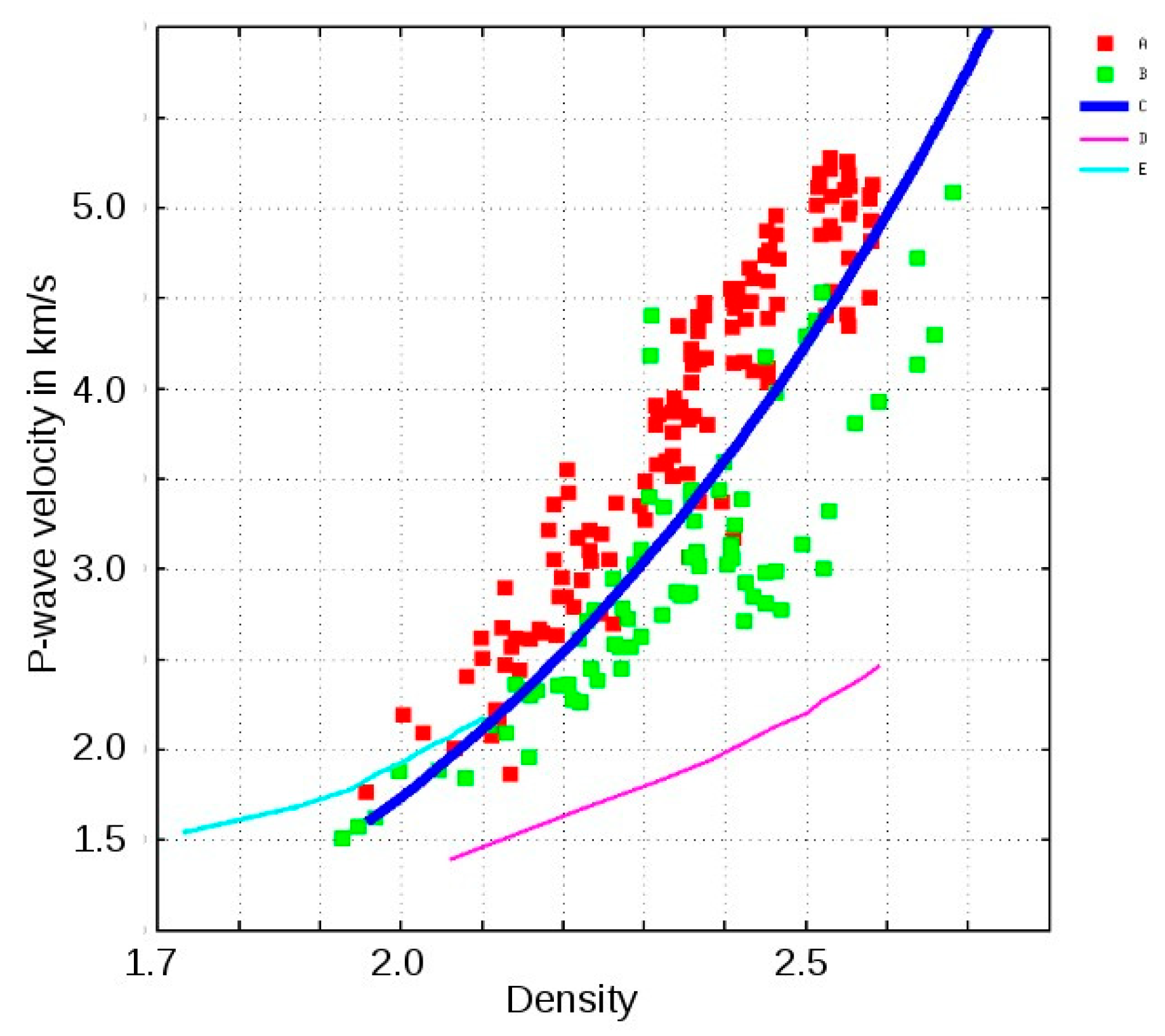
Figure 2. Red circles: Well data from a single basin - DOE Pleasant Bayou #1 and #2 wells, Brazoria Co., Texas(red circles) digitized from Castagna et al. [1] Fig. D-4, Black circles: Equation (2) from Gassmann-Nur model.

C_{ρ} = 2.0568

,

s = 0.1846

- compare with values in Higginbotham et al. [7] for shale and in Table 1.

Figure 2. Red circles: Well data from a single basin - DOE Pleasant Bayou #1 and #2 wells, Brazoria Co., Texas(red circles) digitized from Castagna et al. [1] Fig. D-4, Black circles: Equation (2) from Gassmann-Nur model.

C_{ρ} = 2.0568

,

s = 0.1846

- compare with values in Higginbotham et al. [7] for shale and in Table 1.

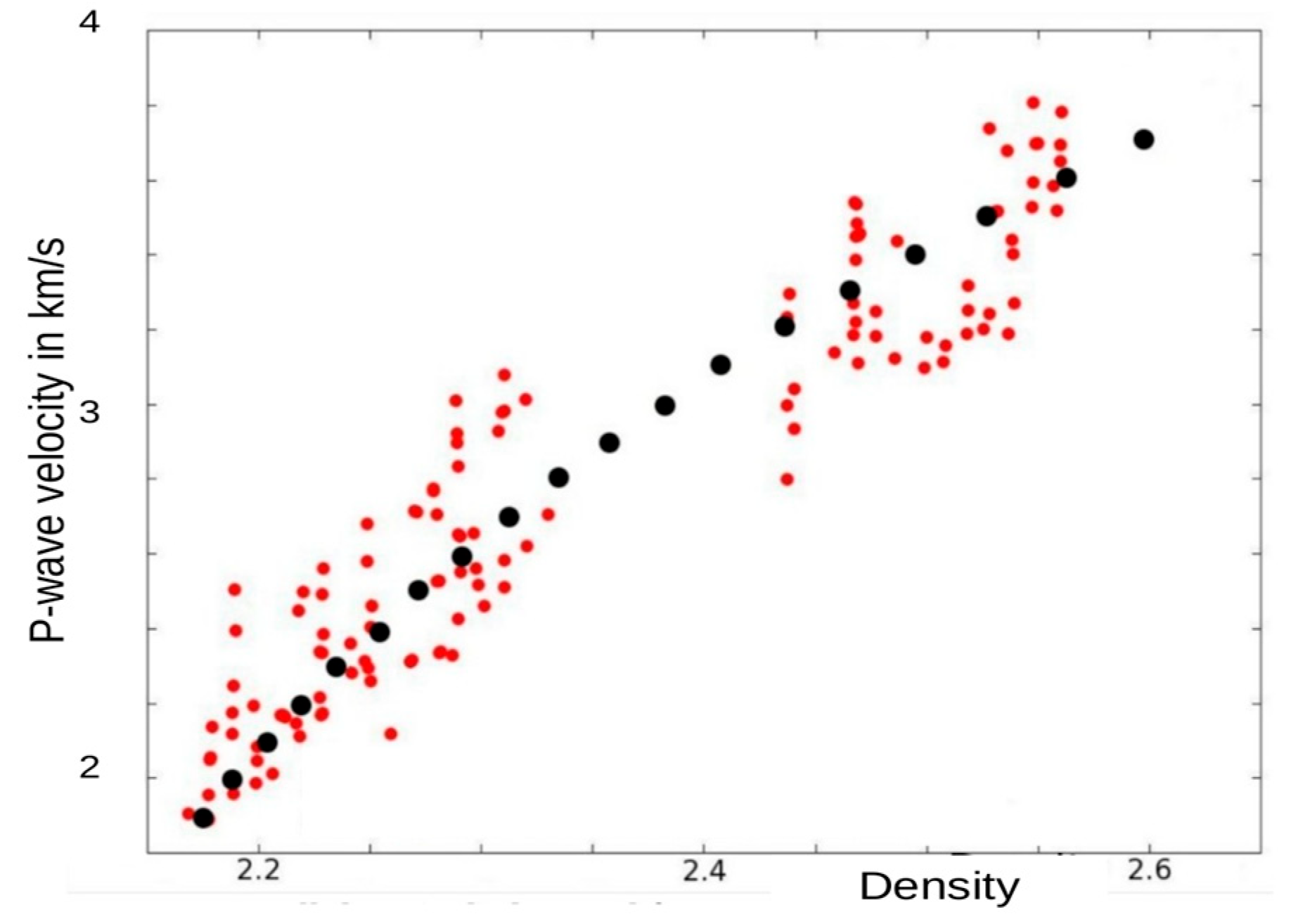
Figure 3. Velocity versus porosity measurements (purple squares) for Clean Silicon Sandstone as reported by Nur et al. [8]. The curves were computed from the GN model with critical porosity set at 0.36 and using published values for quartz elastic constants. The blue line deviating toward lower velocity is for quartz with some clay content.

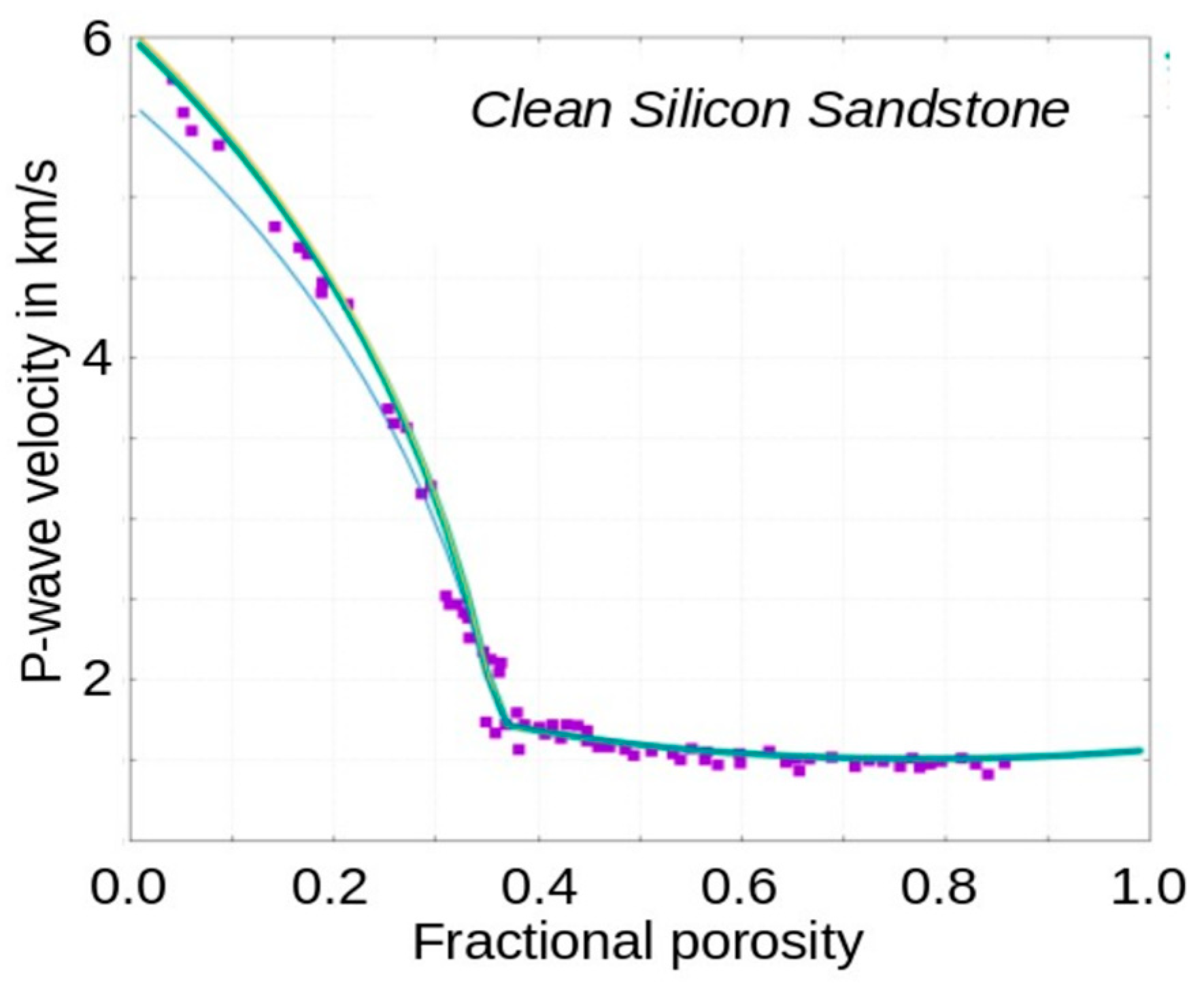
Figure 4. Here the data points of Mondol et al. (2008) for Smectite and Kaolinite are fit with two connected straight lines that meet at what I've called a "crush point porosity" which probably corresponds to the consolidation threshold porosity of Vernik and Kachanov [10,11].

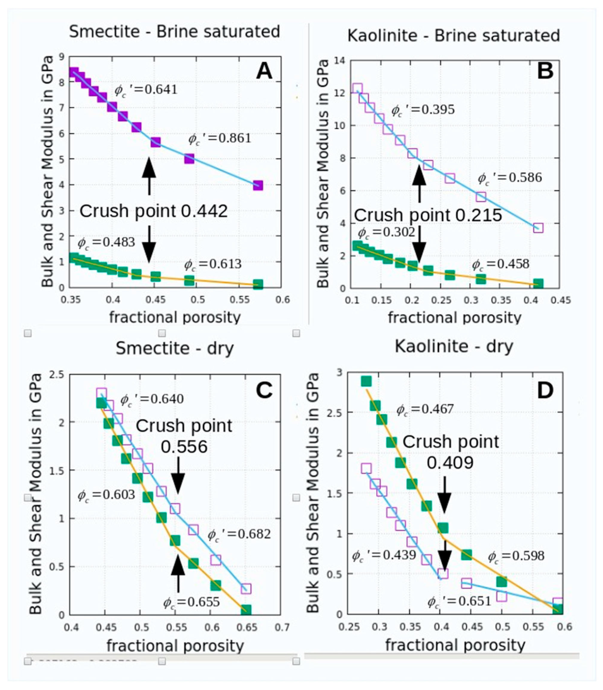
Figure 5. Red and green circles are measured values for sandstone and shale. Color lines are Quartz - Shale earth models with different values of compaction coefficient. Labeling: % smectite (S) or % kaolinite (K), followed by

β

the compaction coefficient. Thick black line is Gardner’s equation. Discontinuity in slope is associated with the crush point porosity of Figure 4.

Figure 5. Red and green circles are measured values for sandstone and shale. Color lines are Quartz - Shale earth models with different values of compaction coefficient. Labeling: % smectite (S) or % kaolinite (K), followed by

β

the compaction coefficient. Thick black line is Gardner’s equation. Discontinuity in slope is associated with the crush point porosity of Figure 4.

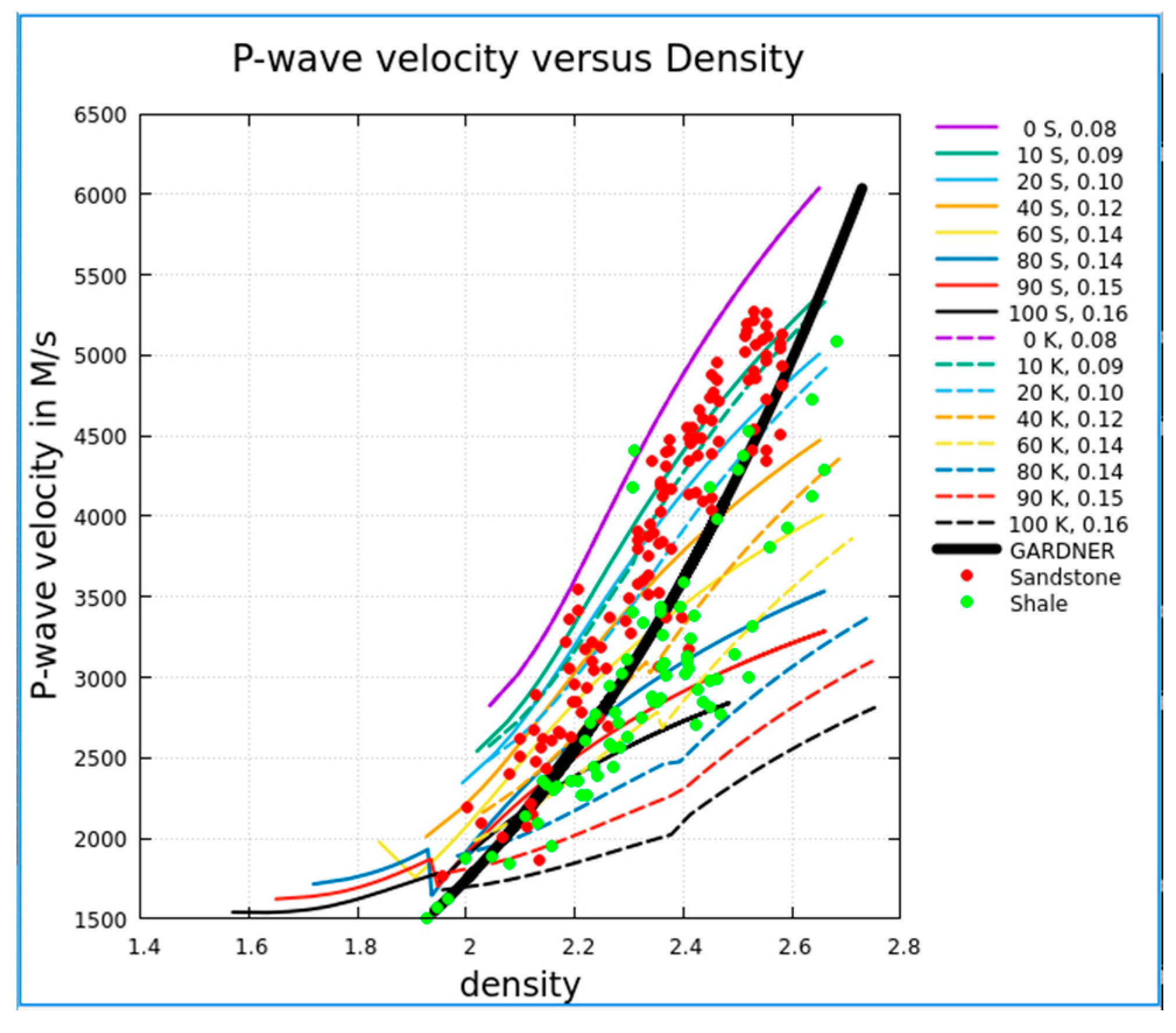
Figure 6. Here the density computed using equation (3) is plotted against the density computed by the earth models for some of the cases shown in Figure 4 as well as others. The match is very good to excellent. Labeling: % smectite (S) or % kaolinite (K), followed by

β

, E indicates the use of an effective fluid bulk modulus. Otherwise the fluid bulk modulus came from Castagna et al. [1] Figure 21.

Figure 6. Here the density computed using equation (3) is plotted against the density computed by the earth models for some of the cases shown in Figure 4 as well as others. The match is very good to excellent. Labeling: % smectite (S) or % kaolinite (K), followed by

β

, E indicates the use of an effective fluid bulk modulus. Otherwise the fluid bulk modulus came from Castagna et al. [1] Figure 21.

Disclaimer/Publisher’s Note: The statements, opinions and data contained in all publications are solely those of the individual author(s) and contributor(s) and not of MDPI and/or the editor(s). MDPI and/or the editor(s) disclaim responsibility for any injury to people or property resulting from any ideas, methods, instructions or products referred to in the content.

© 2025 by the authors. Licensee MDPI, Basel, Switzerland. This article is an open access article distributed under the terms and conditions of the Creative Commons Attribution (CC BY) license (http://creativecommons.org/licenses/by/4.0/).

Copyright: This open access article is published under a Creative Commons CC BY 4.0 license, which permit the free download, distribution, and reuse, provided that the author and preprint are cited in any reuse.

An Interpretation of Gardner’s Equations

Abstract

Keywords:

Subject:

Introduction

Method

Sandstone

Shale

Avoiding $K_{f}$

Quartz-Shale Composite Models

Results

Conclusions

Modified Gassmann-Nur Model

Gardner’s Equation

Funding

Conflicts of interest

Appendix A Path to Gassman’s Equations

References

MDPI Initiatives

Important Links

Subscribe

An Interpretation of Gardner’s Equations

Abstract

Keywords:

Subject:

Introduction

Method

Sandstone

Shale

Avoiding K f

Quartz-Shale Composite Models

Results

Conclusions

Modified Gassmann-Nur Model

Gardner’s Equation

Funding

Conflicts of interest

Appendix A Path to Gassman’s Equations

References

MDPI Initiatives

Important Links

Subscribe

Avoiding $K_{f}$