
Submitted:
01 September 2025
Posted:
03 September 2025
You are already at the latest version
Abstract
In this paper, we will try to study the automorphism and the quantum automorphism groups of some certain class of graphs, directed and undirected. In our previous work, entitled C∗-colored graph algebras, we studied a set of regulated colored locally finite directed graphs Gs with their vertices colored with three colors red, blue, and green, and studied their graph theoretical properties and put a ∗-monoid algebra structure on the set consisting of those kinds of graphs. Here, we will still follow almost the same study, but in a non-color version, and we will study their quantum symmetries. However, we made a slight change to the original graphs considered in our previous work!
Keywords:
graph algebra
; C*-graph algebra
; symmetrizable graphs
; quantum symmetries
; quantum automorphism groups
; quantum permutation groups
1. Notations
Throughout this paper, will stand for the ground field, and it will be assumed to be arbitrary unless otherwise stated.
In this paper, by an edge complement graph , we mean a graph in the usual meaning of the completion in graph theory, but without loops!
Note that in this paper, we will only study symmetries and the quantum symmetries of graphs with an even number of vertices, and if their number of vertices is not even, then we will embed them into an even-dimensional space and then will try to study their properties!
By p and q, we mean any matrices in for such that , and we will not specify them!
By we mean the quantum permutation group in the sense of Wang, generated by magic unitary matrices, and there are infinite many of them!
For and compact (matrix) quantum groups, by we mean the free product of and , and by () we mean the (free) Wreath product of and .
2. Introduction
Mathematics is all about finding patterns, symmetries, and the relations between, or even hidden in, or among the objects. It could be the usual classical ones, or the so-called quantum symmetries and the afterward relations. Starting from groups and the group actions on a vector space V (or just viewed as a set V), the symmetries of V are the self bijections on V preserving the mathematical structures of V. Here the meaning of the statement “preserving the mathematical structures of V”, varies from one structure to another. For example, for a special subset , T will be called a symmetry transformation if for every we have , or for a map , then T will be called a symmetry transformation if , for all , and there are more of these kinds. Hence a symmetry is a transformation that preserves some structures, and the set of all symmetries of any finite dimensional mathematical object O forms a group, presented by , for n the number of elements of O, that consists of automorphisms, the invertible transformations preserving the structure of O.
Now moving to the representation theory, it is not outrageous to mention the most ever important Cayley’s Theorem, where all groups can be functionally represented by a symmetric group. For example we can think about the symmetric group , as the representation of the symmetries of an equilateral triangle, and in another thinking direction, it can be used to represent any group consisting of 3 elements making it much easier to discuss theorems about all kind of groups, and there is a claim stating that every group is isomorphic to the symmetry group of an appropriate object. In order to see this, consider the Cayley graph associated with the given group G, which is constructed from the group of elements and some generating set X (which could be the entire group or a much smaller set, and it could be inverse-closed or not), by connecting elements g of group G (correspondent with the vertices of the graph) to the vertex for each generator x, with the orientation taken from g to .
Definition 1.
Let G be a group, and X be an inverse-closed subset of G. Then the Cayley graph of G relative to X, , will be a simple graph defined as follows:
- i)
- ,
- ii)
- .
Remark 1.
The exact meaning of the Definition 1, is that if and only if there is some such that .
This is exactly where the group action comes in, and by Cayley’s theorem, stating that every group G is isomorphic to a subgroup of the symmetric group on G, and the fact that to any regular action of G on a set X we can associate a Cayley graph such that its symmetry group will be equal to G, and hence we get the desired result.
3. Symmetry Group of a Graph
The symmetry group of a finite graph consists of bijections , for the set of vertices, permuting the underlying vertex set V, and preserving the proper of vertices being neighbors, or not.
Remark 2.
The symmetries of are the permutations leaving invariant the edges, and forming a subgroup of the symmetric group .
Examples 1.
- (a)
- As an introductory and basic example, which is somehow very important for our study, is the empty graph with vertex set , and the automorphism group .
- (b)
- Another example might be the simplex of dimension , for which we have .
- (c)
-
The next logical example to consider could be the polygon in n sides (). Label the set of vertices in counter clockwise order as , and let σ be the associated symmetry of the set of vertices. For example, by taking vertex 1 to the vertex i, then σ must take 2 to the vertex adjacent to i, i.e. to or , and once and are determined, then the mapping σ will be completely determined by using the fact that it has to preserve the distance between every two vertices. Hence, if σ maps 2 to , then it has to map 3 to , 4 to , and so on. And if it maps 2 to , then it has to map 3 to , 4 to , and so on. So there are exactly two symmetries , andTherefore a regular n-gon K (or a polygon of n sides) has symmetries and for , in total, and as it is already apparent, the vertex after n is 1, and hence we have when , and therefore for and , + has to be considered as addition modulo n. And as we notice, the mapping preserves the cyclic order of the vertices, and reverses the cyclic order.And if we think geometrically, will represent a rotation of the polygon about its center through an angle , and represents a reflection in the diameter lying midway between vertices 1 and i. And it is clear that is the identity permutation, and represents reflection in the diameter through vertex 1. Then the symmetries , and , for can be expressed in terms of two basic symmetries. Let us call them , and , so thatwhere α represents a rotation through angle and moves each vertex i to . For any integer represents a rotation through angle , and hence . Furthermore we have , and effect on vertices 1 and 2, it follows that . Thus the symmetries are given by , for .And it is clear that , and . And by considering , and . Hence , and therefore we have obtainedas the group of symmetries of the regular n-gon K, where α represents a rotation through an angle and β represents reflection in the group , and as it is already known, any group of elements that has the same structure as in group G, will be called the dihedral group of degree n and will be denoted by , and hence we have shown that .
- (d)
- Now let us move to that oriented n-gon, which easily could be verified that its symmetry group is , because if we choose a vertex i and denote its image , then as the permutation σ leaves invariant the edges, with their orientation, then σ must map to , to , and so on, and must be an element of the cyclic group, in remainder modulo n notation .
4. Automorphism Group of (Directed) Graphs
Every finite graph has a group of self bijections on , which is identified with , for n the number of distinct elements in . Now consider a subgroup of consisting of the mappings preserving the adjacency and the nonadjacency between the vertices , and call it the automorphism group of , and denote it by .
For example, for a graph on three vertices and three edges, we have .
Definition 2.
Define the automorphism group of a (finite) graph Γ as as a subgroup of , for the transpose of σ in .
Now by looking at any unitary matrix as a permutation so that , we can embed in such that be an injective group homomorphism.
Consider the finite graph and let be the automorphism represented by the unitary matrices in of the graph with n vertices and let be the adjacency matrix of . Then it is not too difficult to verify that .
Remark 3.
So far, until this step, we have recovered a result stating that one can look at every element of the automorphism group of the finite graph Γ on n vertices as an matrix.
4.1. Quantum permutation groups
Following a question raised by Connes “asking if there is any way of thinking about the quantum version of the usual permutations and the permutation group , and what would it be?”, in 1998, Wang came with a sophisticated positive answer saying that quantum permutation groups do really exist and could be defined as follows in the framework of the principles of noncommutative geometry and the GNS constructions, and the formal definition is as follows.
Definition 3.
The quantum symmetric (permutation) group is the compact matrix quantum group, where
Remark 4.
- i)
- Matrix with entries s from a non-trivial unital -algebra satisfying relations and , as in the Definition 3, will be called a magic unitary, such that all its entries are projections, all distinct elements of a same row or same column are orthogonal, and sums of rows and columns are equal to 1.
- ii)
- Note that from the magic unitary matrices, the ones with noncommutative entries are of quite importance to us, and in these cases, not all entries need to be noncommutative with each other. Some of them might be just 1! Of course, if in any row or column, we have 1, then the other entries have to be zero in the same row or column.
Now in order to characterize the functions from to , i.e. , we will use the same setting as in and we define
and as is a subgroup of , then by applying the contravariant functor (the function functor), we will get the surjection , where the quotient is the set of permutations that preserve adjacency, which is the requirement for the permutations contained in , and the quantized version [3], due to Banica, considered by , such that the diagram
5. Symmetrizable Matrices
The concept of symmetrizable matrices mostly have been developed in order to study, or along with studying, some of the objects in Lie theory. For example we can name the generalised Cartan matrices, which are some sort of important classes of symmetrizable matrices.
Definition 5.
[8] Let be an real matrix. Then will be called symmetrizable if there exists a real diagonal matrix , for , such that is symmetric. Then will be called the symmetrization.
Remark 5.
There is another related notion where the entries of the symmetrizable matrix are integers, and in that case will be called a symmetrizable integer matrix (SIM).
Actually it is not too easy to verify if a given matrix is symmetrizable or not. Hence there have been developed some techniques throughout in order to combat this issue, such as the rational cycle condition, the absolute trace, the sign symmetric, and the existence of some evaluation values, which will be explained in this review paper. There is the following definition.
Definition 6.
[8] An real matrix will be called sign symmetric if we have for all .
Let us recall that a generalized Cartan matrix is an integer matrix for , such that
- i)
- if ,
- ii)
- if ,
- iii)
- if and only if .
And C will be called symmetrizable if there exists positive real numbers , for , such that for all .
Example 3.
Now by applying the above characterization, we see that is a symmetrizable generalized Cartan matrix. Let us now apply the Definition 5 and to see if we will be able to verify it or not!
For and , consider . Then we have
and as the characterization in Definition 5 suggested, in order for B to be symmetrizable, the requirement of to be symmetric is necessary and sufficient. But it is not clear if (3) is symmetric or not! Hence we have the following criteria.
Criteria 5.
[8] Let . Then for any sequence of numbers , if we have
for any real sign symmetry matrix , then A will be a symmetrizable matrix.
Remark 6.
So, in order to complete the Example 4, we use the cycle condition from the Criteria 7. As B is sign symmetric, hence We have , and there are no other cycles.
Remark 7.
- (i)
- All symmetric matrices are symmetrizable.
- (ii)
- Not all the permutation matrices are symmetric, and hence they mostly are not symmetrizable. For example , is not symmetric, and hence is not symmetrizable. But is symmetric and by a certain choice of the diagonal elements , it is easy to see that it is symmetrizable. The matrix A and its generalizations are important to us, and are called , and for its generalizations in [14,15,16], as it will also be called the same in this paper as well.
- (iii)
- [8] For a real sign symmetric matrix , there is another weaker criteria, stating that A is symmetrizable if and only if there exist , for such that satisfies.
- (iv)
- After knowing the symmetrizablity of a given real sign symmetric matrix , we can evaluate its symmetrization by defining the real symmetric matrix by , which is symmetrizable and is the symmetrization of A.
- (v)
- There is another criteria in order to check if an sign matrix is symmetrizable or not, and that is if there exist a diagonal matrix such that is symmetric, then is symmetrizable. For example for the matrix B from Example 4, we have for any .
6. Looking for a Well-Structured Criteria for Symmetrizability of Matrices
Consider the generalized Cartan matrices , and . It easily could be verified by using the Criteria 7 and Remark 7e, that A is symmetrizable and B is not, and this happened by just changing the places of and in the symmetrizable matrix A, in order to obtain the not symmetrizable matrix B!
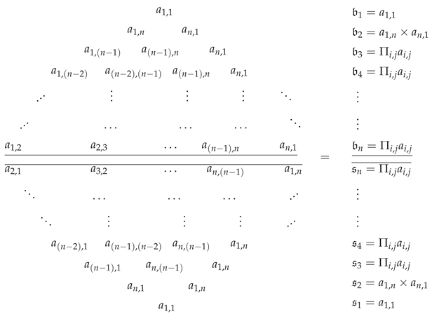
As the Criteria 5 has to be valid for any such sequence of numbers, hence we can propose the above cycle, which is nothing else than the original cycle condition, but the generalized one. For an matrix we have the above -row diagram where the middle line will be called the symmetry line. Meaning that the sign symmetry matrix will be called symmetrizable if and only if the diagram is symmetric over the symmetry line!
Remark 8.
- Note that in the above diagram, by a row, we mean the multiplication between the entries involved in each row, and because of the simplicity, we just have omitted the multiplication signs.
- In the above diagram, there are rows, but as the first two and the last two rows will clearly be equal, hence the actual number of rows in the diagram will be , and the diagram will be called the -row diagram.
For example for the generalized Cartan matrix B we have
which certainly is not symmetric over the line of symmetry, and hence it is not symmetrizable.
Remark 9.
Any real matrix with at least one zero row or column will automatically be symmetrizable.
7. Symmetrizable and Quantum Symmetrizable Graphs
As our knowledge allows, the notion of a symmetrizable graph hasn’t been coined out until now. Hence, to do this we have to divide the class of graphs into directed and the undirected ones, and play with their adjacency matrices. However, this method might not work for the undirected ones, as the adjacency matrix in this case will be always symmetric and hence symmetrizable.
7.1. Directed graphs
The directed graphs could be seen as a weighted graph, or just a not simple directed graph with multiple oriented edges between their vertices, and loops.
7.1.1. The simple connected directed graphs
A directed graph will be called simple if its edge set contains no loops, and there are no multiple edges between two vertices, and will be called locally finite connected if every vertices of it are connected to their adjacency vertices and the degree of any vertex is finite. For example, the graph illustrated below in Section 7.1.1, is simple locally finite connected directed graph
As in [14,15,16], let us call the graph in Figure Section 7.1.1, . Note that the adjacency matrix of will be as follows
and as it contains zero row and column, hence
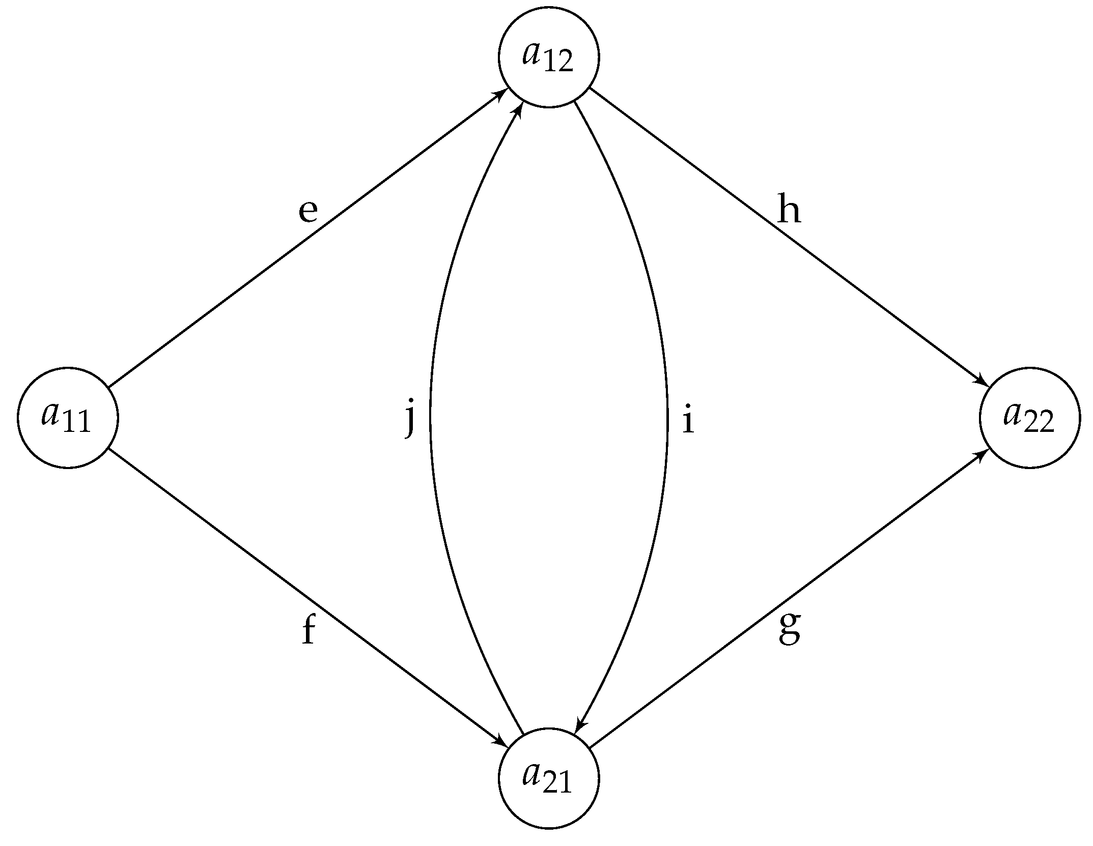
Figure 1.
Directed locally connected graph associated with .
Definition 7.
A simple locally finite connected directed graph will be called symmetrizable if and only if its adjacency matrix is symmetrizable.
Remark 10.
- i)
- In other words, and in completion of the Definition 7, one could say that a locally finite connected simple directed graph is symmetrizable if its automorphism group is non-trivial.
- ii)
- The simple directed locally finite graphs having at least one sink or source vertex will automatically be symmetrizable.
Examples 7.
- 1.
- For example, for graph we have , which is non-trivial and hence is symmetrizable.
- 2.
-
Now consider the following simple locally finite connected directed graphClearly the automorphism group of is the trivial group, and hence it is not symmetrizable. We can see this by looking at its adjacency matrix , which is not symmetrizable as well. Because we have .
- 3.
-
Now consider the following locally finite directed graph .It’s adjacency matrix is equal to , and to observing that it’s only commuting matrix is not a noncommutative magic unitary, is not too difficult!But later on, in Section 7.2.2, we will see that the undirected version of possess quantum symmetries!
Figure 2.
Connected directed simple graph .
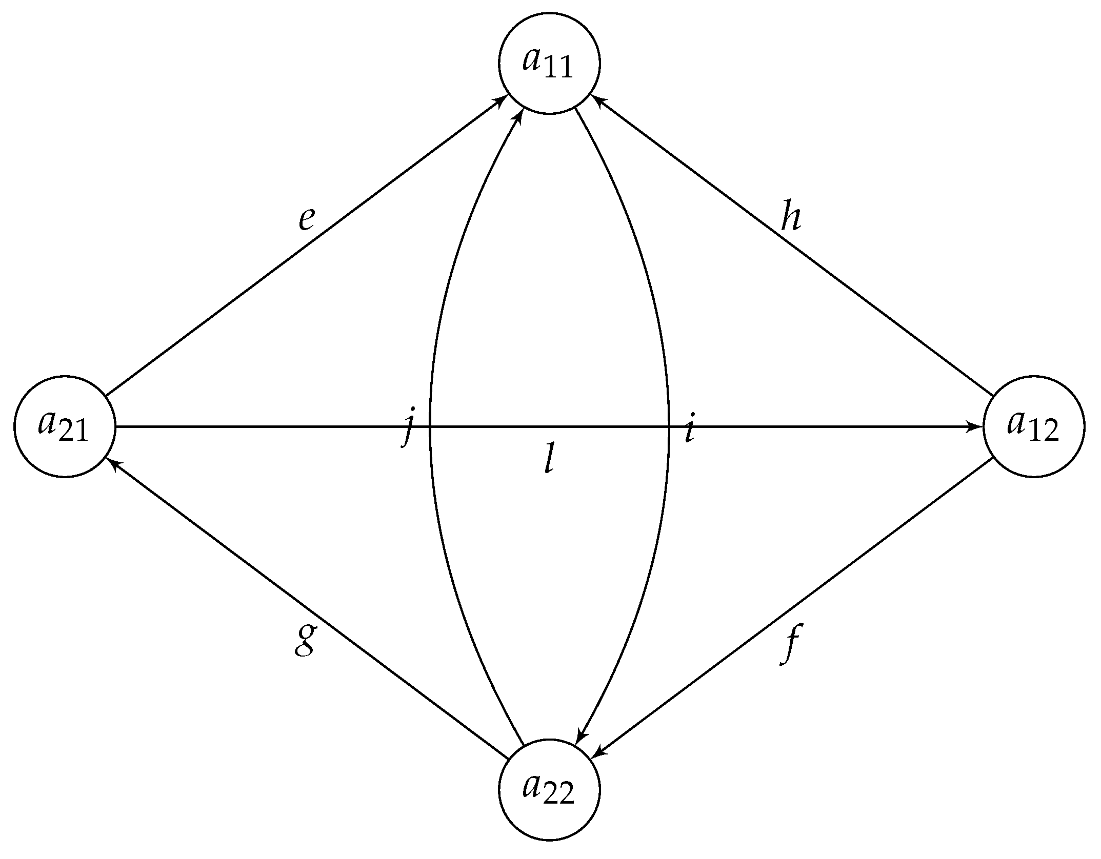
Figure 3.
Two connected graph .
So, the only question that arises here could be the following.
Question 8.
- 1.
- Are there any counter examples of a simple locally finite connected graph Γ, such that its automorphism group is trivial, and its adjacency matrix is symmetrizable?
- 2.
- Or is there any sign symmetry matrix (with diagonal entries 0) such that it is symmetrizable, but the automorphism group of the associated directed graph is trivial?
Note that the only commuting matrix with matrix A is , for . And for u to be a magic unitary, we should have and , which will provide us with the commutative trivial magic unitary matrix, and hence A is not quantum symmetrizable and has no quantum symmetry and its quantum automorphism group will be the trivial group, and we may have the following definition.
Definition 8.
A simple locally finite connected directed graph Γ will be called quantum symmetrizable, if and only if its quantum automorphism group is non-trivial.
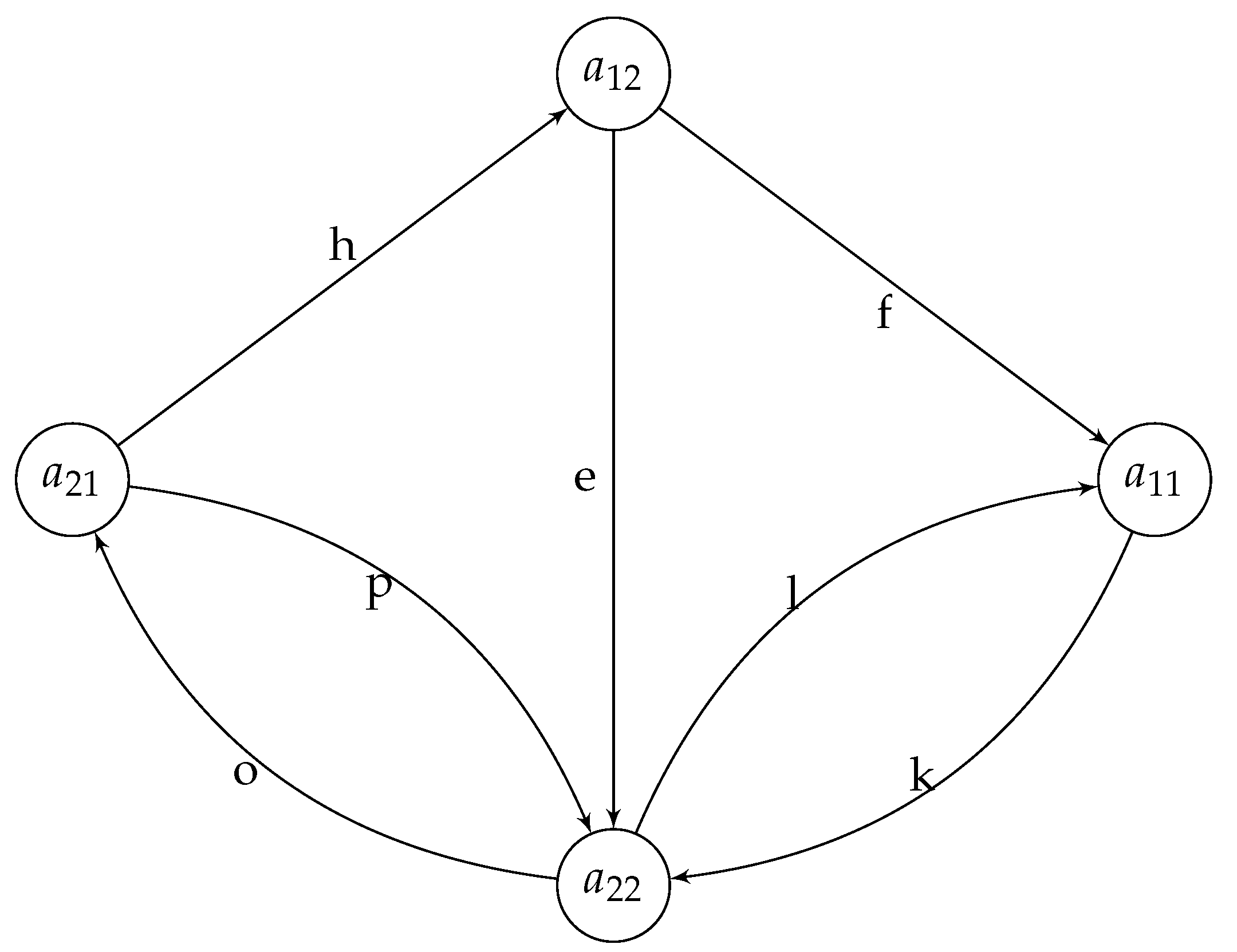
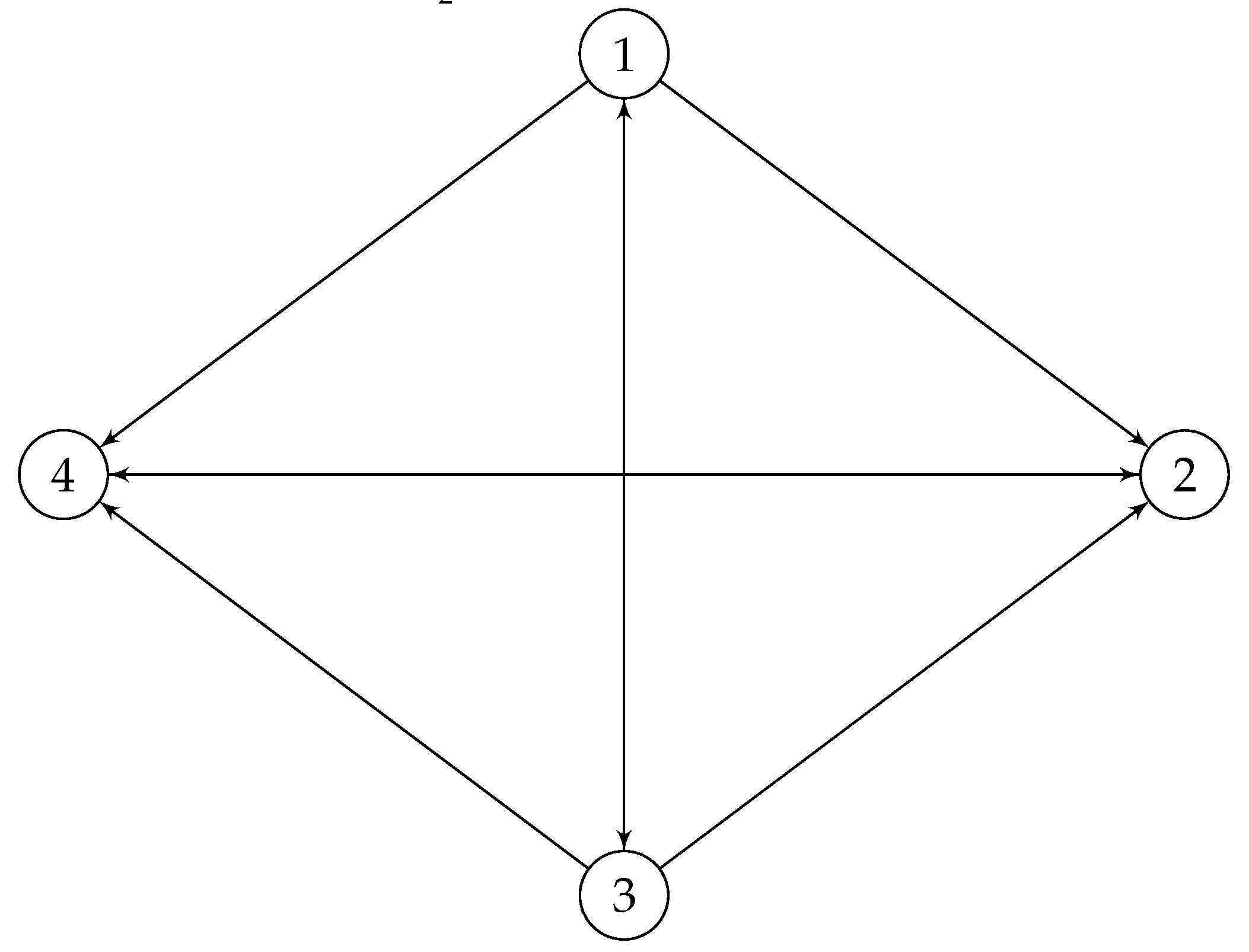
Let us study two more examples. Consider the following directed graph
Figure 4.
Connected directed simple graph .
It is clear that , and its adjacency matrix is symmetrizable, and the only commuting matrix with is
, for , which is not a magic unitary for any a! Hence has no quantum symmetry!
But with a small change, we have the following graph,
Figure 5.
Connected directed simple graph .
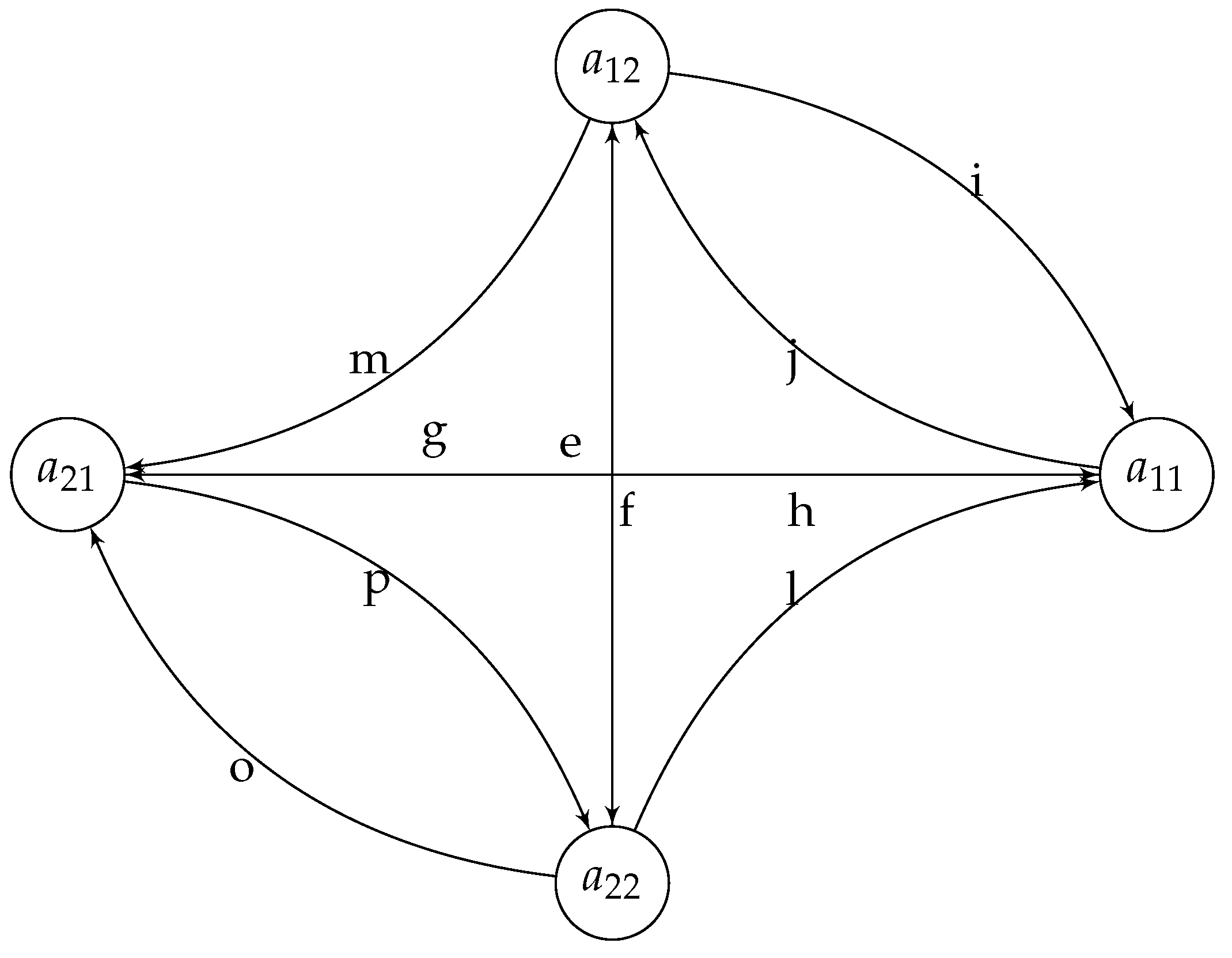
and it is not difficult to observe that the adjacency matrix is symmetrizable, and its commuting matrix has to be something like , for , and it is clear that will be magic unitary only in the case where we have and , which is the trivial one, and hence the quantum automorphism group is trivial and it possesses no quantum symmetry, and it is not quantum symmetrizable.
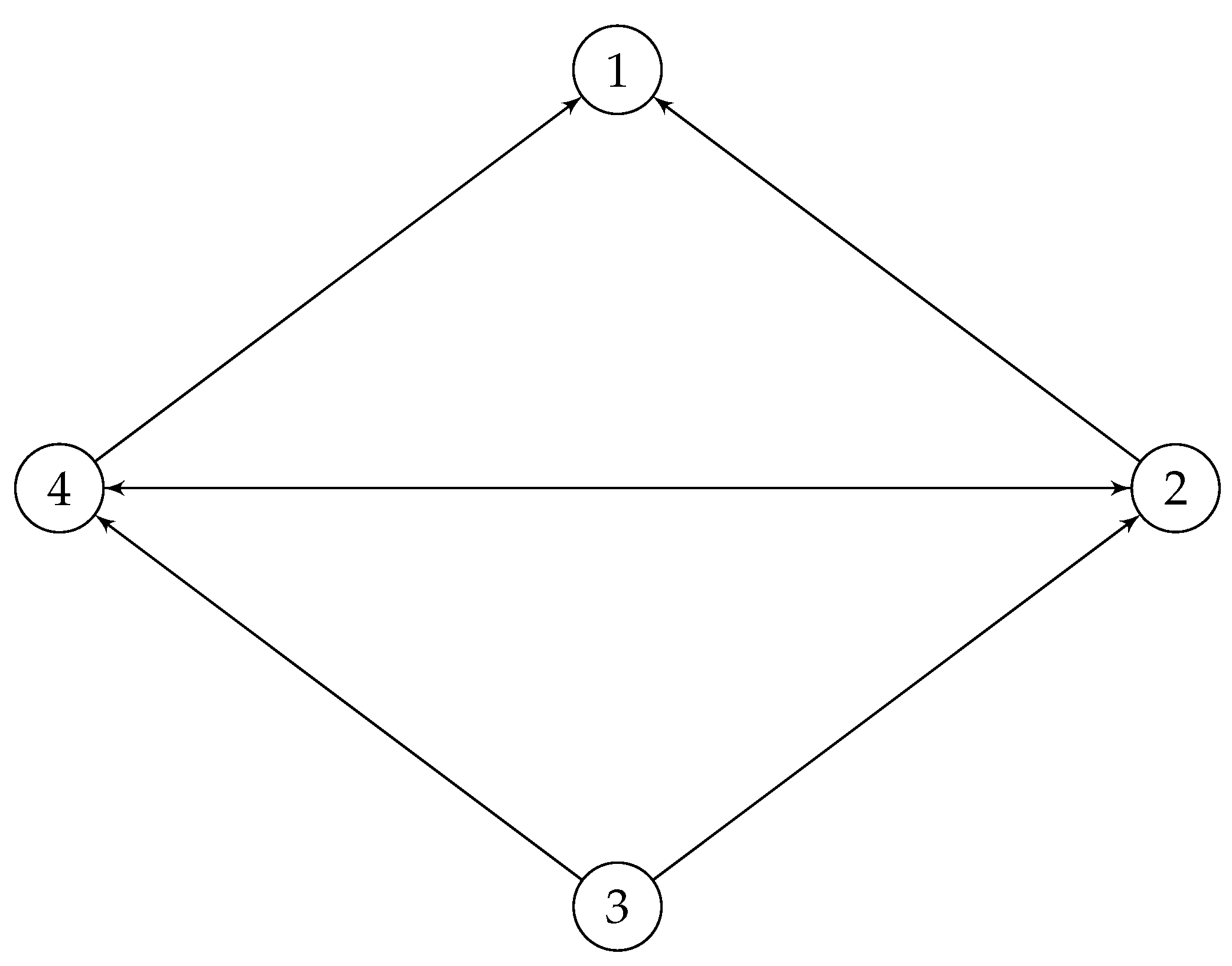
Now let us see a not symmetrizable and not quantum symmetrizable directed graph. Consider the following graph
Figure 6.
Connected directed simple graph .
As it is clear is not symmetrizable, and is trivial. On the other hand the adjacency matrix is also not symmetrizable, and we see that in this case, still the statement in Definition 7 holds. The plan is to find a counterexample or an example that satisfies the conditions stated in Question 8.
7.2. Undirected graphs
The situation is completely different for the undirected graphs. This case has to be divided into two interrelated sub classes.
7.2.1. Weighted undirected graphs
Weighted undirected graphs will be considered in our next paper or in the updated version of the current paper.
7.2.2. Not weighted undirected graphs
Note that the not weighted undirected graphs are the simple weighted undirected graphs. Here as in the Section 7.1, a simple graph will be referred as a graph without any loop and multiple edges. And since, in this case the adjacency matrices are always symmetric, hence they are symmetrizable. But of course not all of them should be regarded as being symmetrizable. Hence we propose the following definition.
Definition 9.
An undirected graph (where u goes back to the undirected case) will be called symmetrizable, if its automorphism group is non trivial.
Example 9.
For example, the following example is not symmetrizable.
It is not too difficult to see that the automorphism group of is trivial. This could be proved by using the fact that an automorphism of an arbitrary graph Γ has to preserve the distances between the vertices , as well as the triangles involved.
Figure 7.
Locally connected (undirected simple) graph .
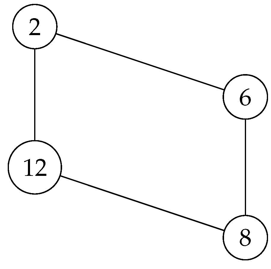
Example 10.
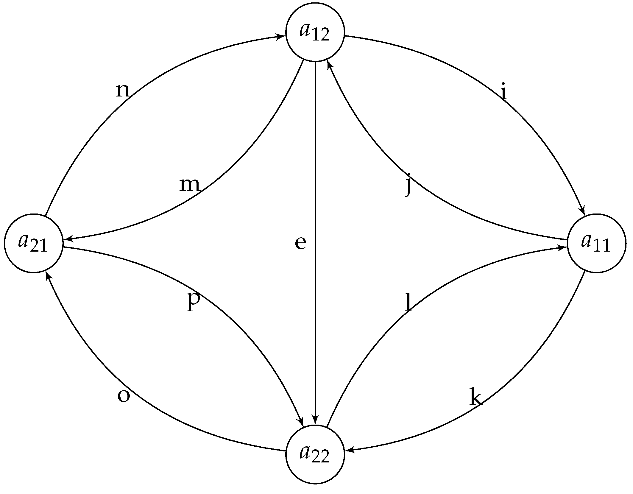
Consider the undirected version of presented in Figure 8.
Note that the adjacency matrix of the above graph is , has a unique noncommutative commuting magic unitary
associated with! And hence, possess quantum symmetries, and this will be the start point!
Figure 8.
Two connected graph .
Remark 11.
Later on, we will use 12, in order to obtain a new set of regulated graphs that possess quantum symmetries!
In [19] as an application of the following theorem, also from the same paper, it has been proved that the Clebsch graph does indeed have quantum symmetry.
Theorem 1.
[19] For any finite graph Γ, if there exists two nontrivial, disjoint automorphisms and with orders respectively, then Γ has quantum symmetry, and one gets a surjective *-homomorphism
Now consider the following graph which has been studied in [17] as a colored undirected graph. Here, following the purposes of this paper, we drop the colors and try to study its usual version.
Figure 9.
Three connected graph .
Note that the Clebsch graph is the folded 5-cube graph introduced in [19]. But analogously, one may see as in some sort of folded graph (but we still don’t know the exact structure)!
Figure 10.
Four connected graph .
Proposition 1.
has disjoint automorphisms.
Proof.
It is clear to observe that the following non-trivial disjoint elements of , belong to .
□
Corollary 1.
does not have quantum symmetries, meaning that its quantum automorphism group is trivial!
Proof.
Note that one may associate the following adjacency block matrix to
for , the following matrices
From which, the graph associated with possess quantum symmetry, as the only commuting matrix with it is the noncommutative magic unitary . But, However, the graph associated with does not possess any quantum symmetry, as the only commuting matrix with them, is not a noncommutative magic unitary, and in general is not a noncommutative magic unitary in any case! □
Remark 12.
Note that, the tensor product and direct sum of magic unitary matrices will still be magic unitary.
Corollary 2.
- i)
- Let be a block matrix of the form , and let be the associated graph, and let and be the associated graphs with and respectively. The claim is that if any of or have no quantum symmetries, then also will have no quantum symmetries!
- ii)
- On the other hand, if both of and have quantum symmetries, then will also have quantum symmetries!
Question 11.
Needs more attention Is the result obtained in Corollary 1 in a false direction with the fact proven in Theorem 1 [19], or there shouldonlyexisttwonontrivial distinct automorphisms?
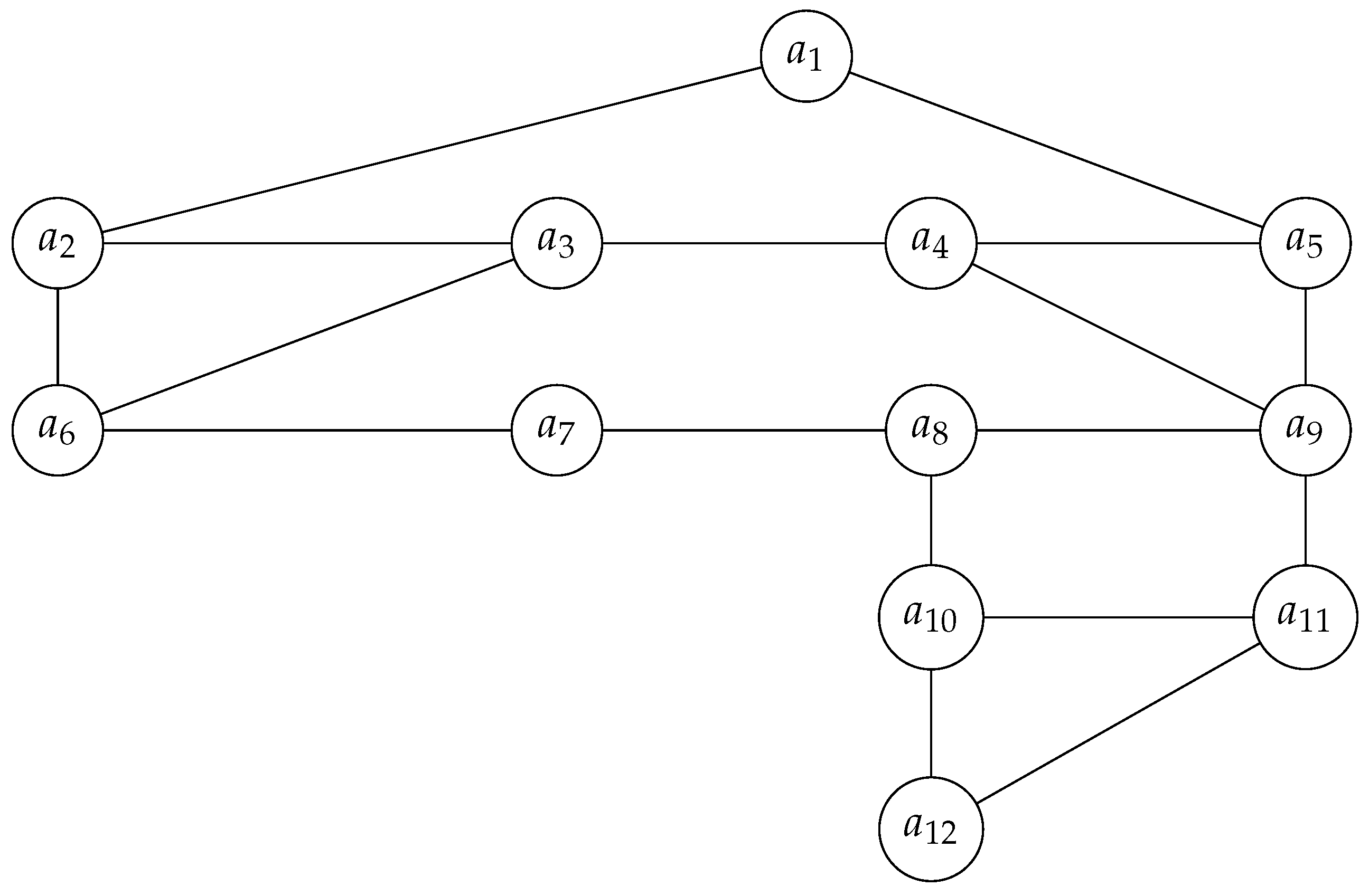
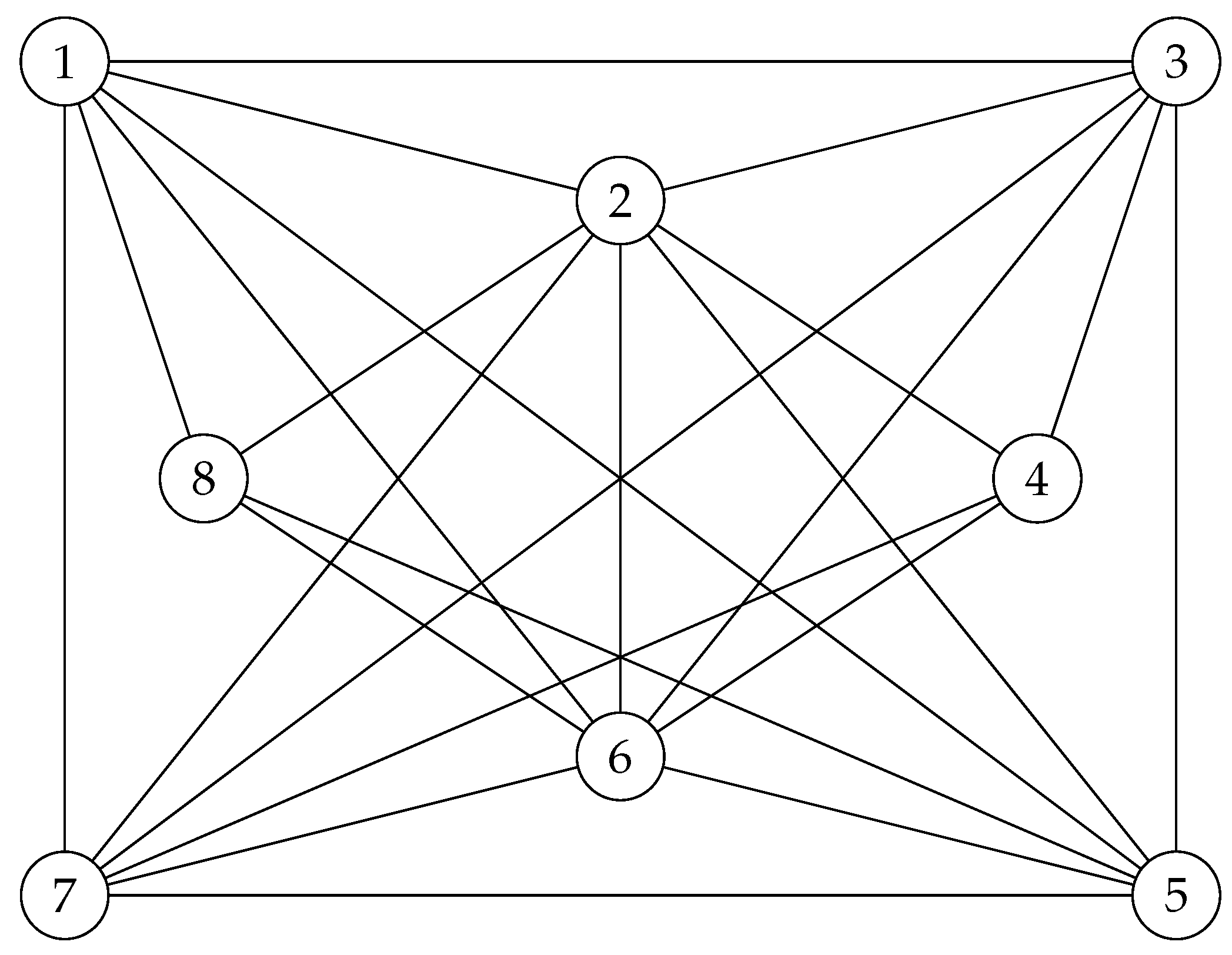
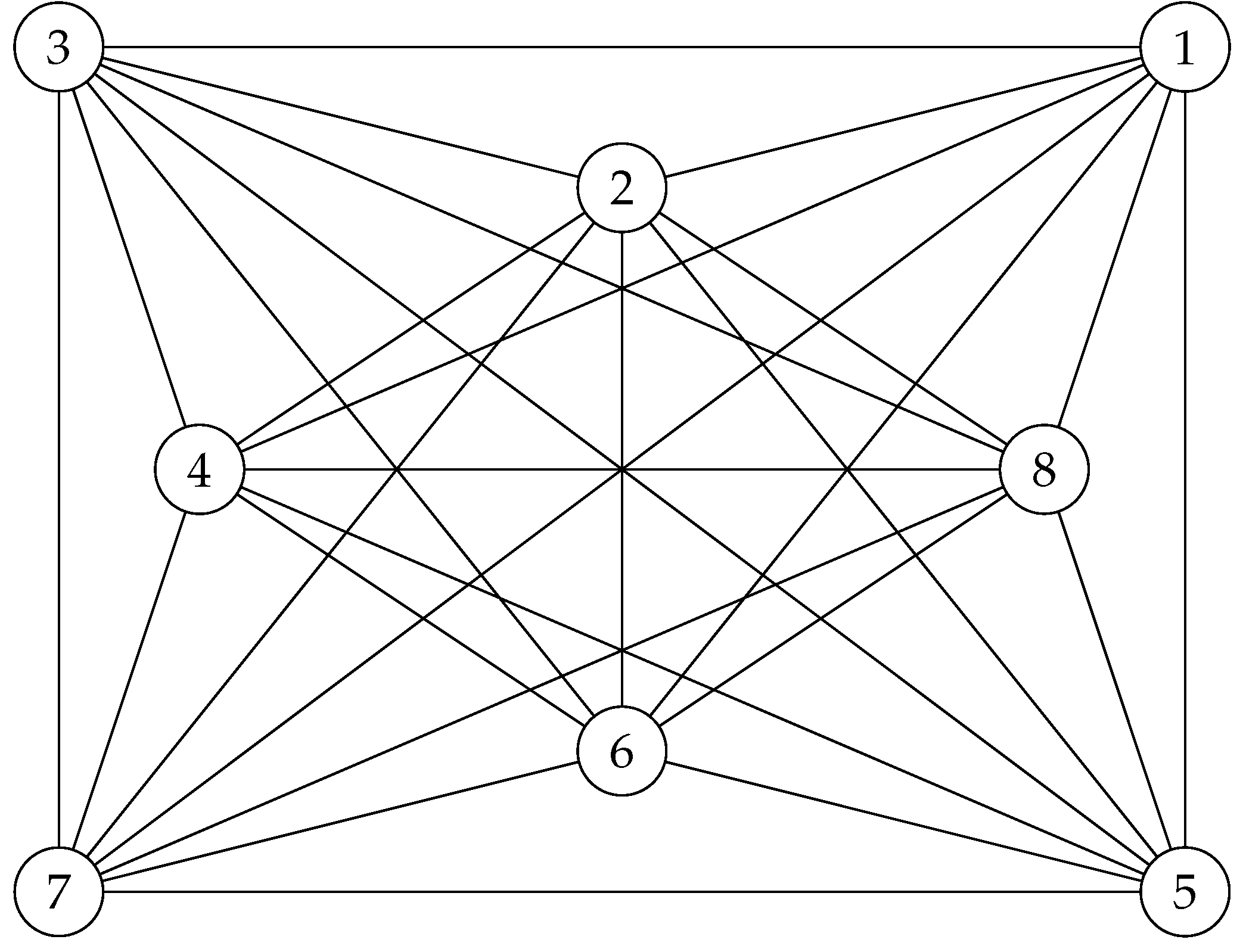
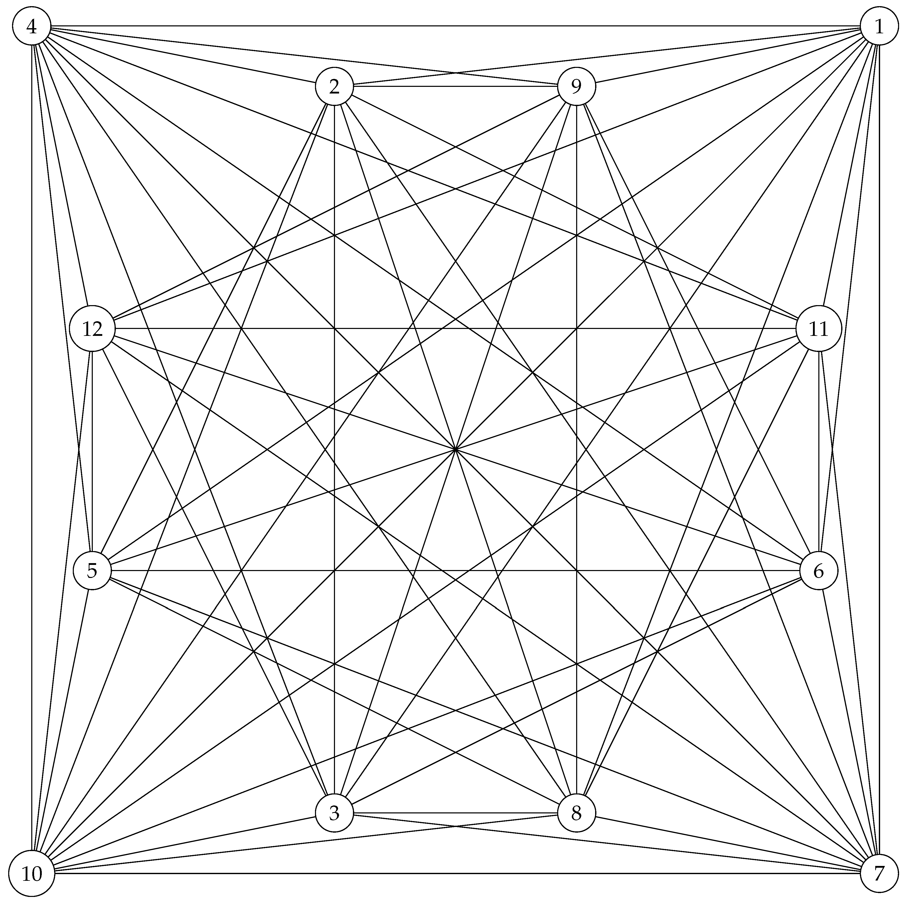
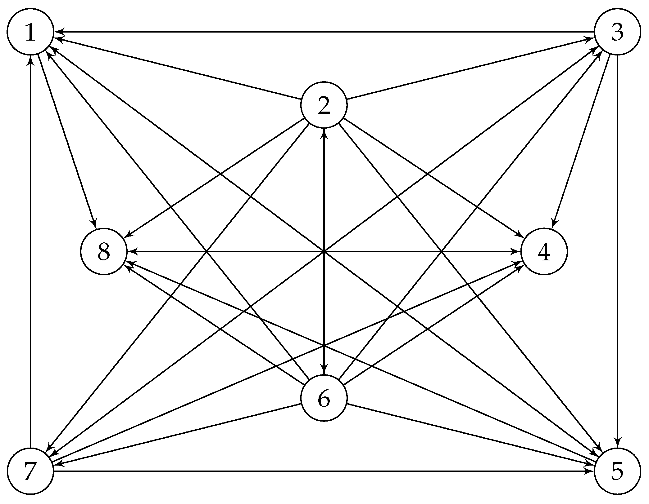
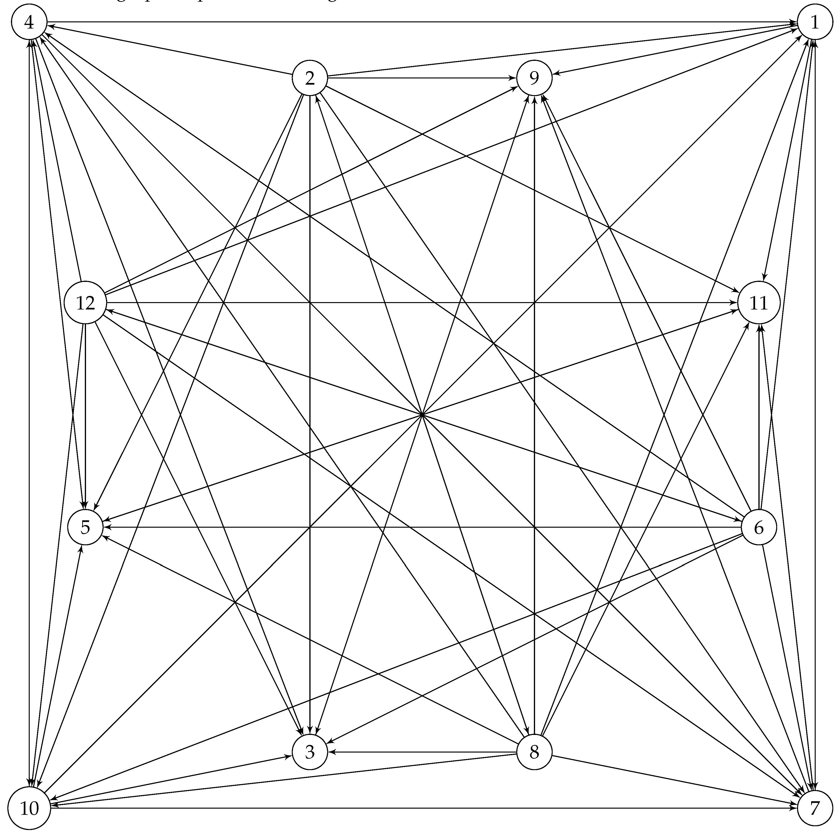
In order to come up with an answer to the above question, consider the following graph, which is the undirected uncolored version of the locally connected directed graph introduced in [17], with its outer layer totally connected and removing the edge between 4 and 8, and connecting 2 and 6! Also notice the swipe between vertices 3 and 1 and vertices 4 and 8!
Figure 11.
Four connected graph .
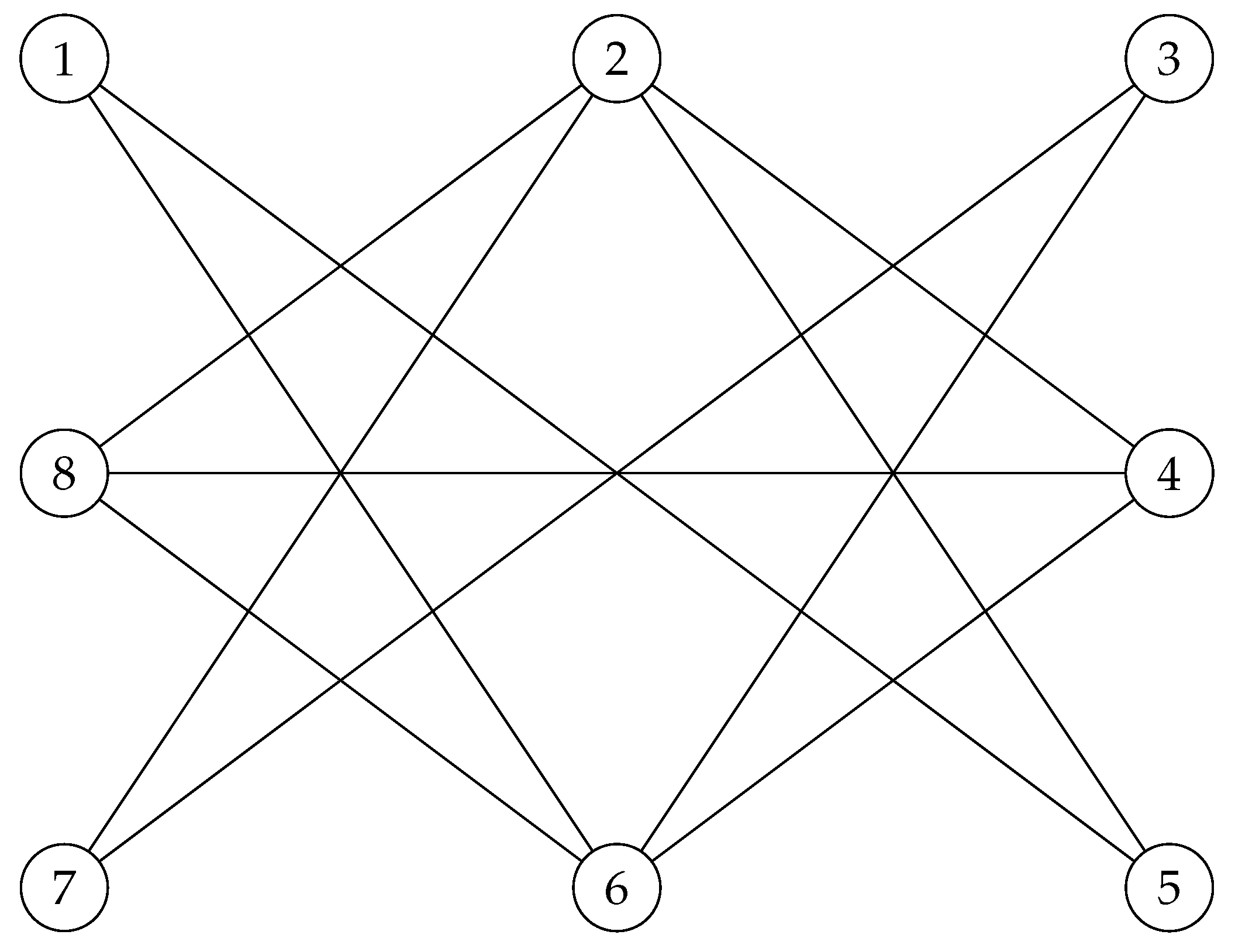
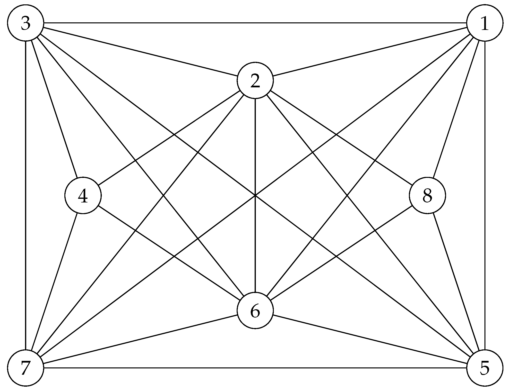
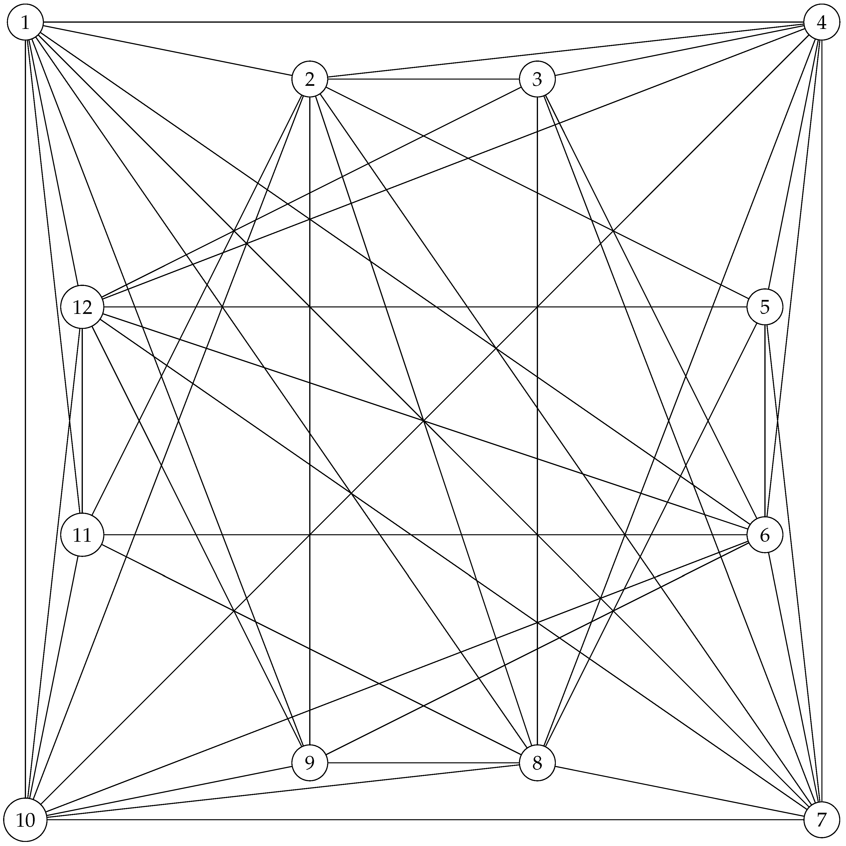
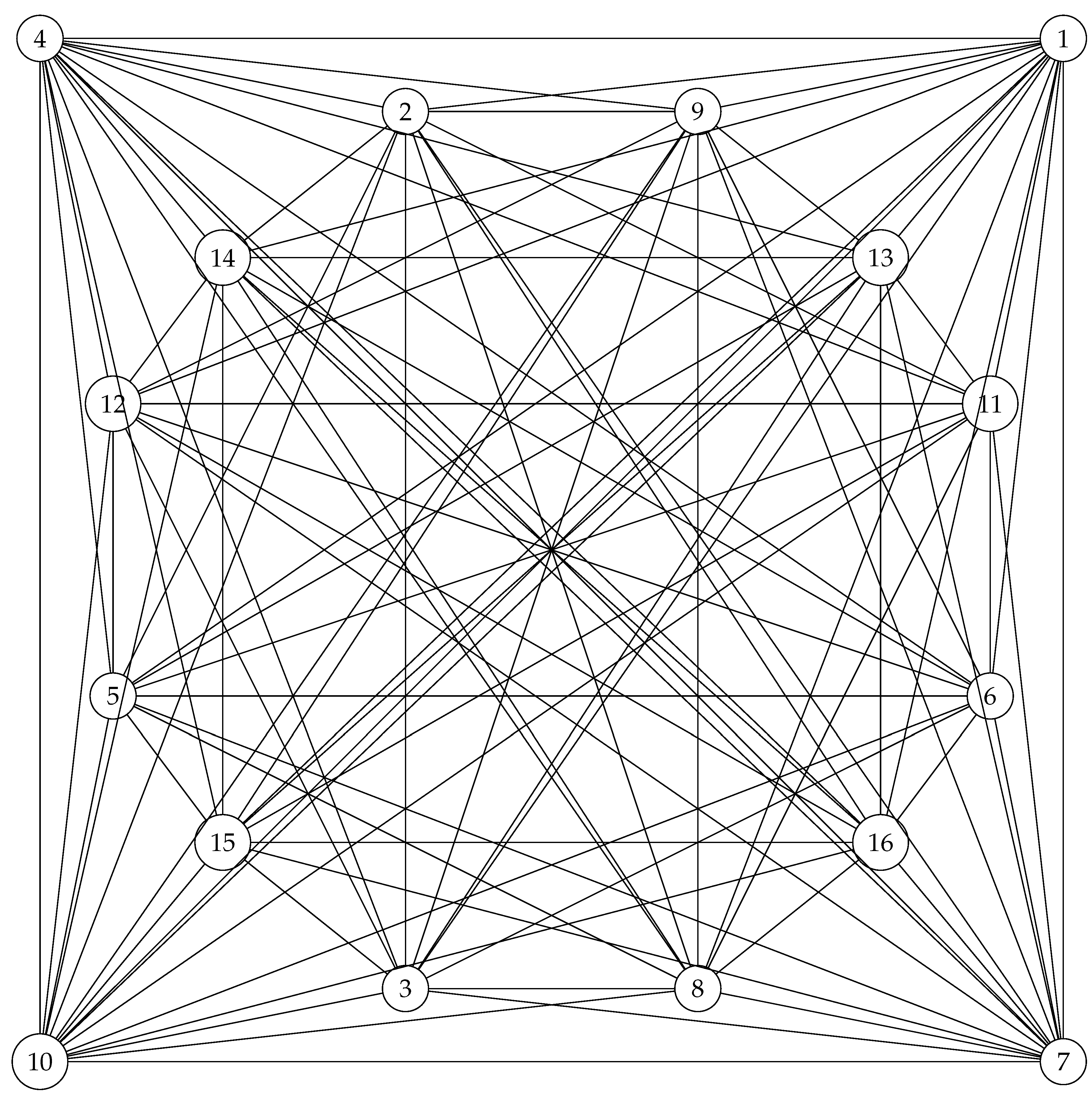
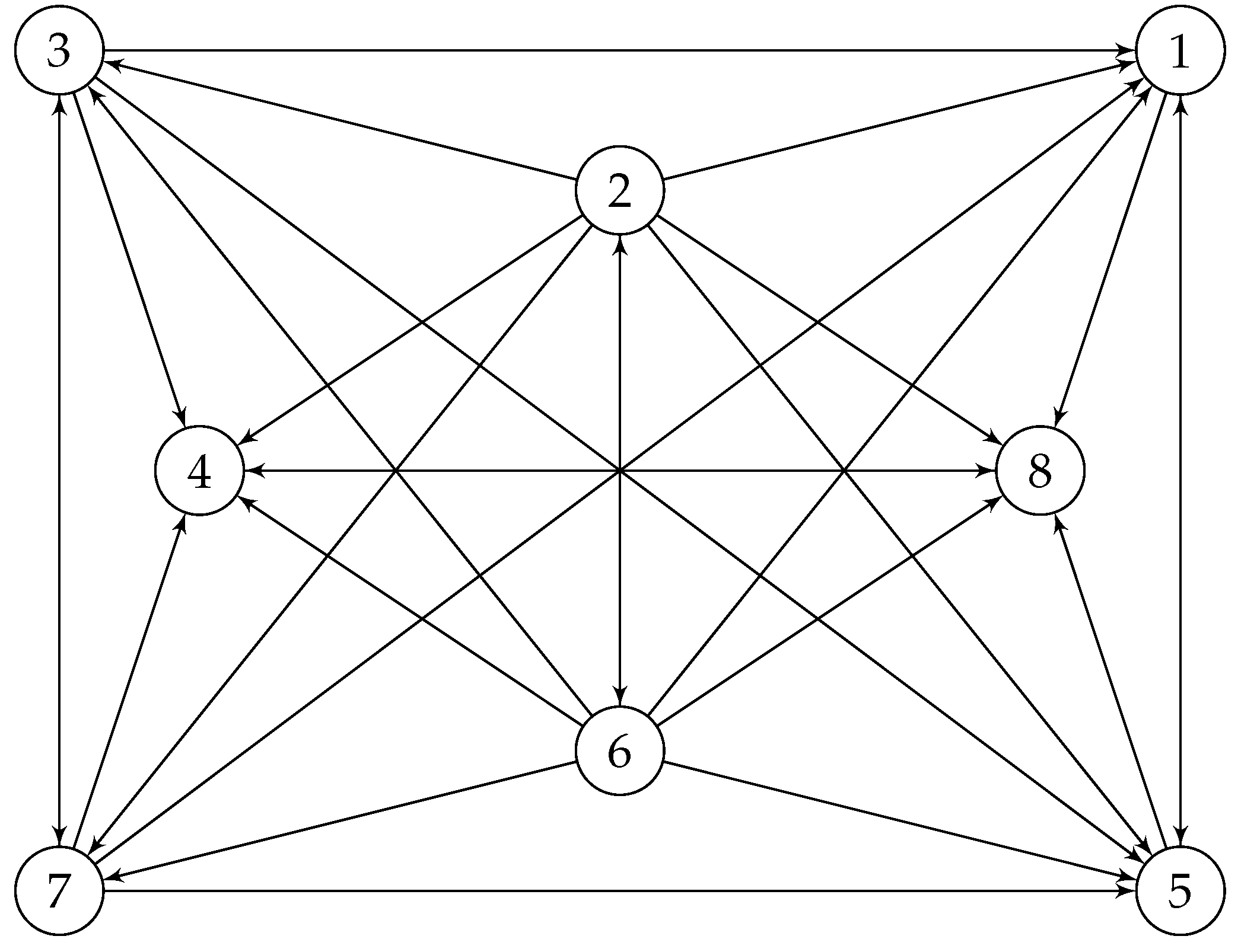
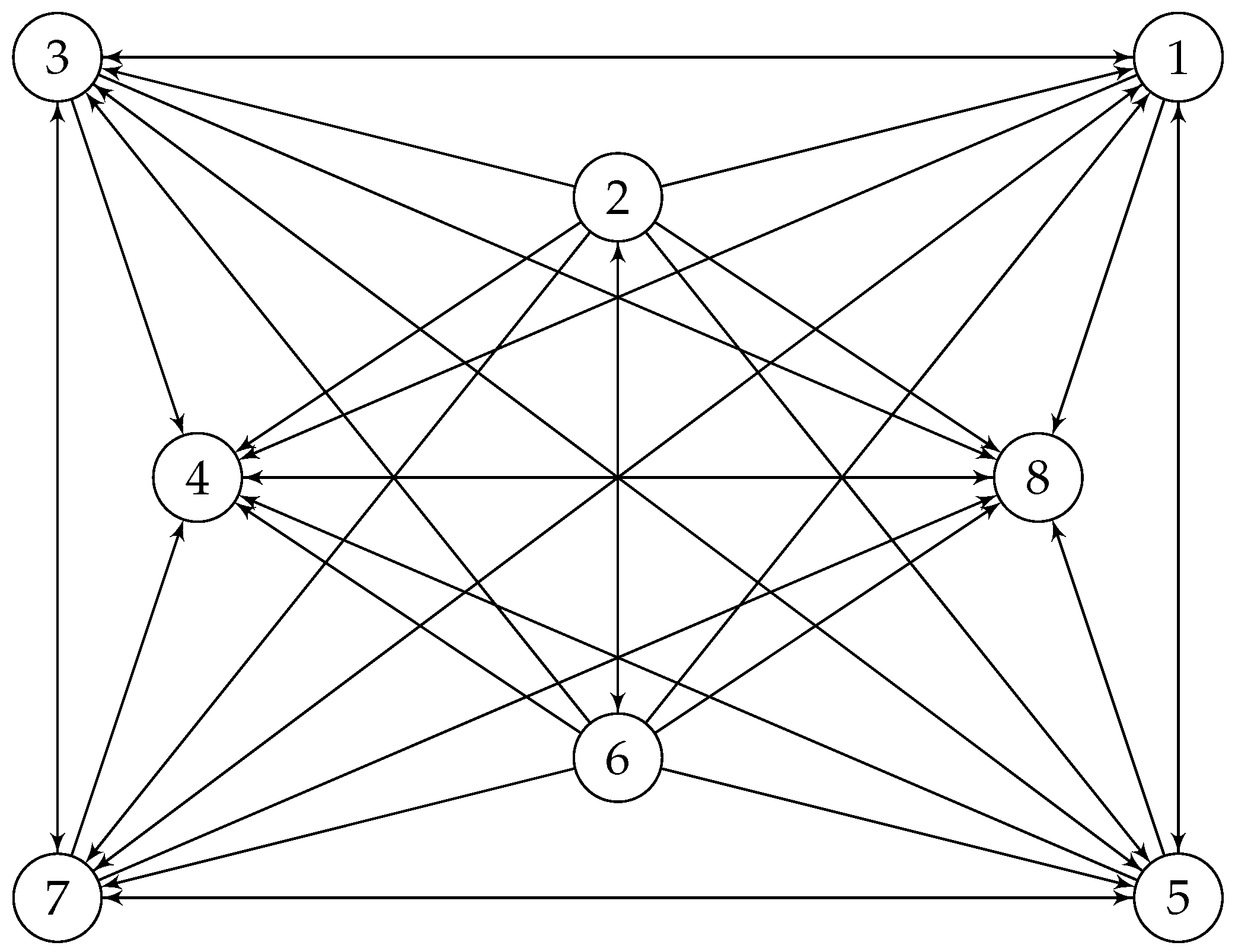
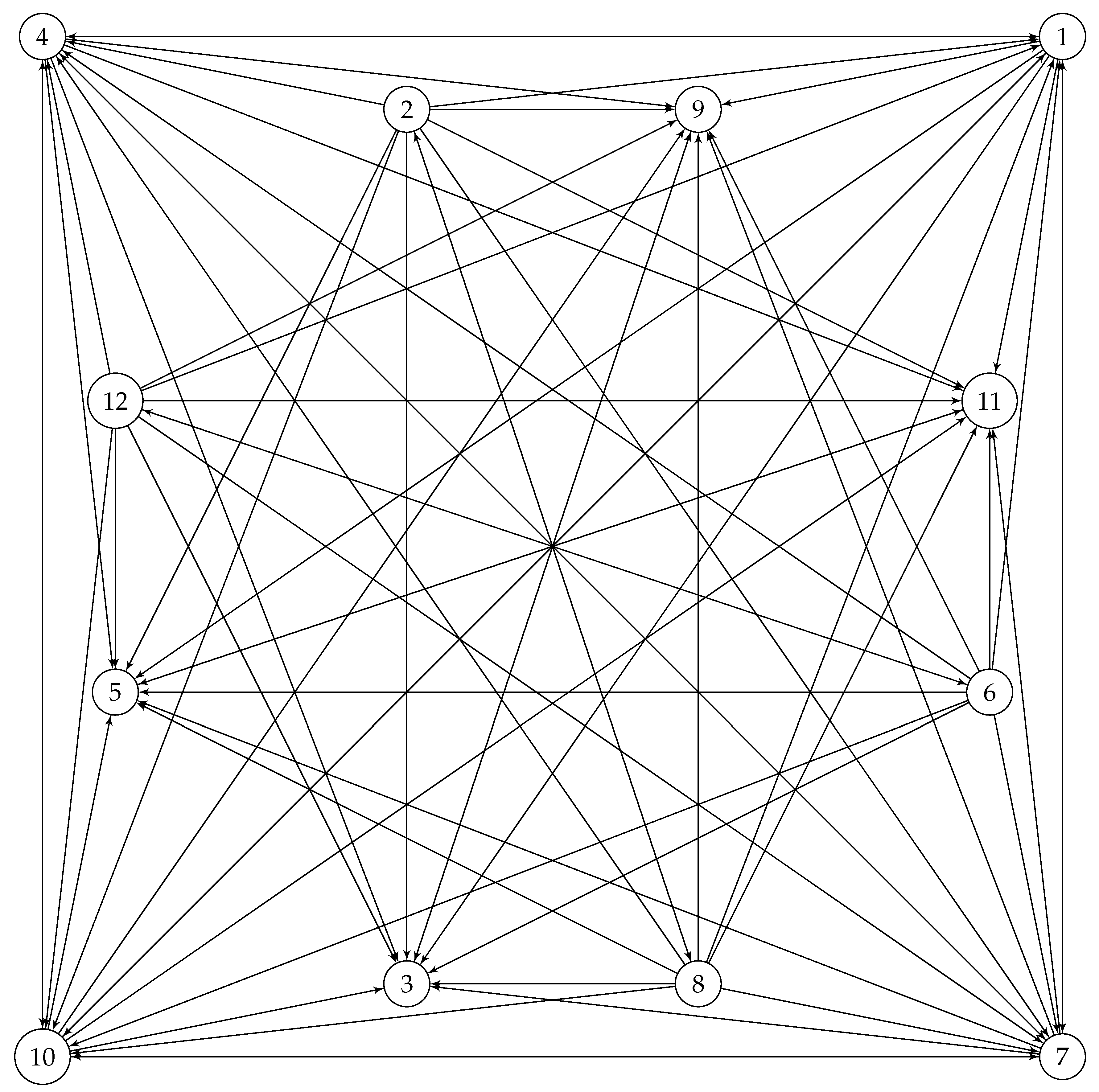
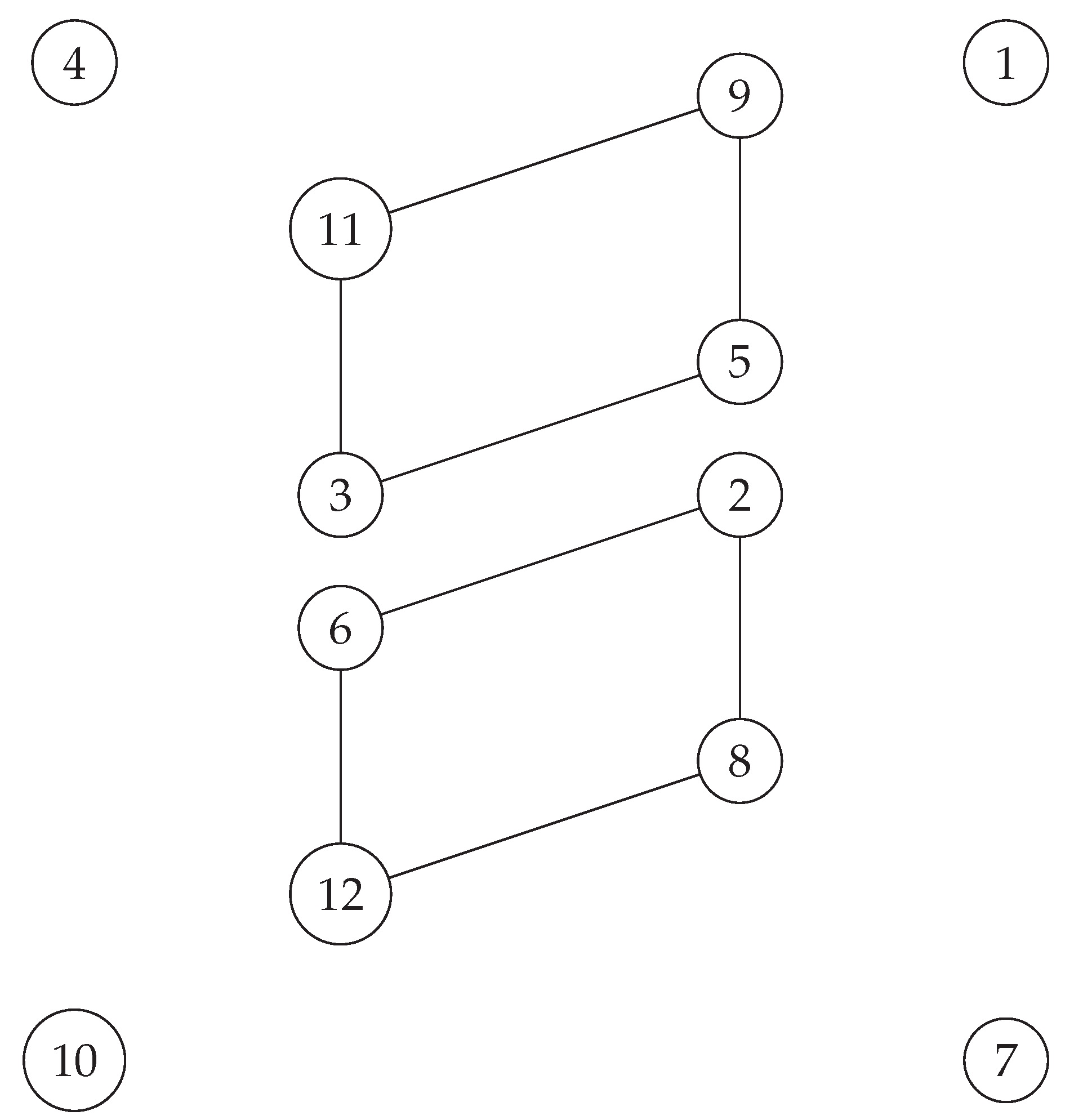
And with a rotation , one obtains the following graph , which will be our main object for a lattice arrangement.
Figure 12.
Four connected graph .
Proposition 2.
has disjoint automorphisms.
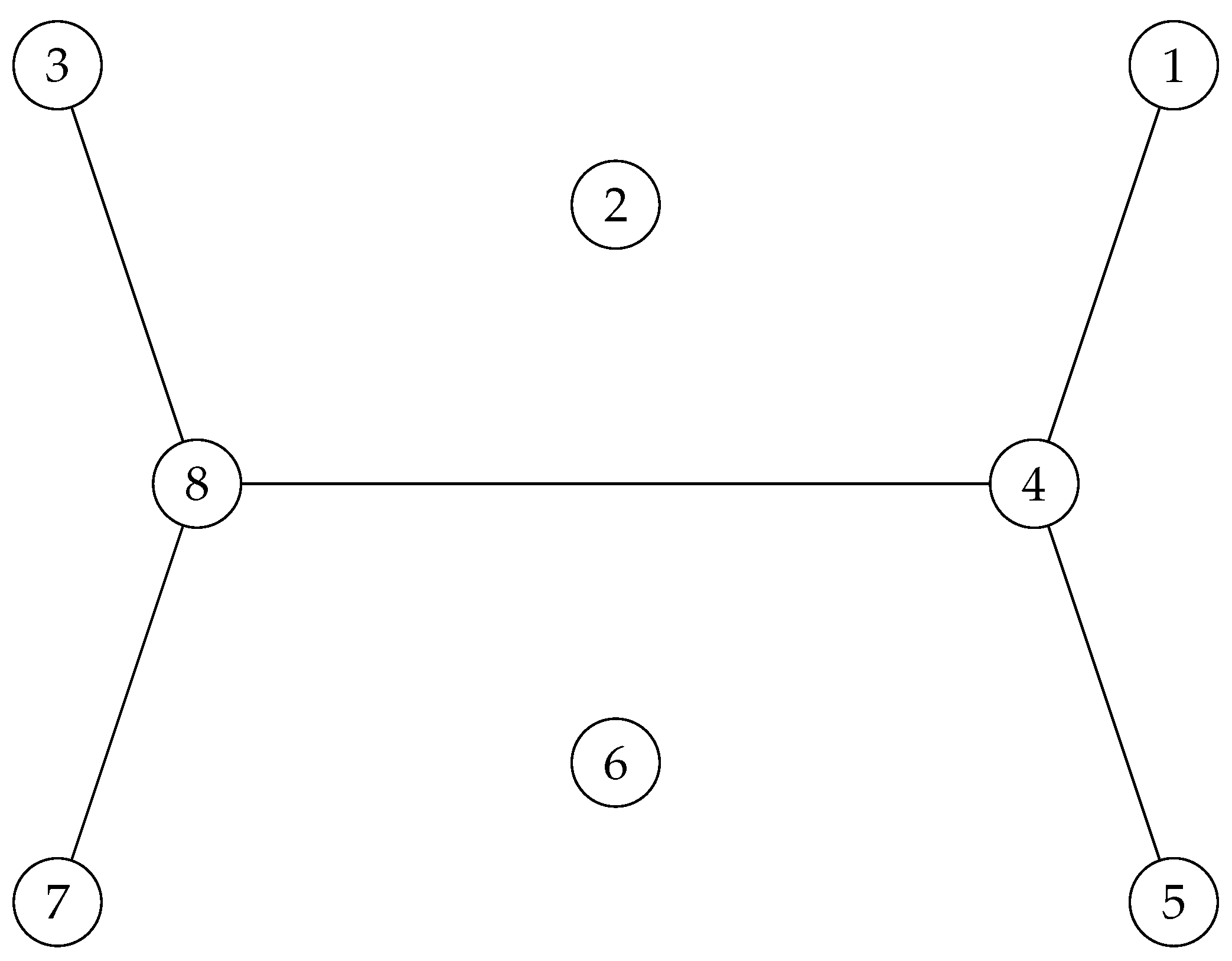
Proof.
Note that the edge complement of is as follows.
It is known that one should have , and it is not too difficult to see that is generated by and . Hence, also has to be generated by two disjoint elements of , and they are as follows.
□
Figure 13.
.
Remark 13.
- i)
- It is known that almost all trees have quantum symmetries![11]
- ii)
-
But in order to complete the statement stated in the first point, let be a tree with n number of vertices. This means that its adjacency matrix is in the space of matrices.
- (a)
-
Now, if is a union of disjoint trees, then it has quantum symmetry in the same space as its adjacency matrix lives. For example, one may easily observe that the following graph , consisting of two disjoint trees andFigure 14. and from left to right.
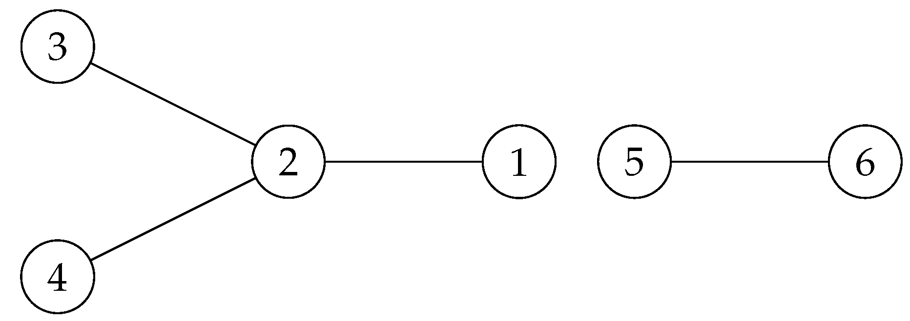 possess quantum symmetry, since the only commuting matrix with its adjacency matrix is the following noncommutative magic unitaryNote that has quantum symmetry in any quantum permutation space with !
 - (b)
-
But, if you just consider , it has no quantum symmetry in and . However it has quantum symmetry in with !For example, in , the following noncommutative magic unitary is the only commuting matrix withAnd we believe that this is true for any single tree without loops!Note that has no quantum symmetry in and , but it possess quantum symmetry in . Because its adjacency matrix, commutes with the following noncommutative magic unitary and this is the only one.
Corollary 3.
Almost all single simple trees with adjacency matrices in , have quantum symmetries in for . But they do not possess any quantum symmetries in with .
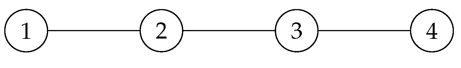
We have the following lemma from the Ph.D. thesis of Simon Schmidt [20].
Lemma 1.
[20] For Γ a locally finite (directed) simple graph, consider its edge complement (described as in the Notation section) with . Then is trivial if and only if is trivial.
Corollary 4.
does have quantum symmetries, and there is a surjective *-homomorphism .
Proof.
Note that one may associate the following adjacency block matrix to .
for , the following matrices
From which, just to one can associate a noncommutative magic unitary and the graphs associated with possess no quantum symmetries.
However, by using Lemma 1, and the fact that is a noncommutative magic unitary for as follows
one may conclude that also is a noncommutative magic unitary!
Note that one may say that refering to an unproven claim can not provide us with a rigorous answer, and that might be correct! But in the next remark, we will try to present a proof in its usual sense!
The existence of a surjective *-homomorphism is a direct result of Proposition 2. □
Remark 14.
- i)
- Note that in the proof of Corollary 1 our insist in using Lemma 1, was just giving some justification to the mentioned Lemma. However, in the next point of the current remark, we will present the usual way of proving such results!
- ii)
-
Note that to the adjacency matrixone can associate the following unique noncommutative magic unitarymeaning that possess quantum symmetries and its quantum automorphism group is non-trivial.
Remark 15.
- 1.The results obtained in Corol
- 2.
- Note that, we have , and as has been proved in [20], we have and . We will use these facts later on while working in higher dimensions.
Remark 16.
- i)
- Hence, in an early response to the question raised in 13, one may have an early inclusion that the statement stated in Theorem 1 has to include “only(and this is exact) two distinct automorphisms”!
- ii)
- Note that in [17], we proved that the colored directed version of , which we called , does not possess any quantum symmetries. This also could be true for the directed not-colored version of .
- iii)
- Note that the process of moving from to is almost as same as the process of equipping the set of locally finite colored directed graphs introduced in [17], as the set of locally finite colored directed graphs with the vertex chromatic number 3 (colored specifically red, blue and green).
- iv)
- The only difference is that here we will get a *-monoid algebra structures on undirected graphs, and it makes it a bit difficult to deal with the operations introduced in [17]!
- v)
- Note that, here we still will use the notations of inner and the outer layers of the lattice array for , with the only difference that our graphs are no longer colored! So we will just work with the outer and the inner layers and , respectively, instead of colors!
- vi)
- In the inner layer of , let be the set of vertices with degree and be the set of vertices with degree . Then we have .
- vii)
- Note that, just for our uses in this paper, we are going to divide the set of vertices into separate and disjoint union sets of vertices and . Where by and we mean the nearest and the farthest (by the mean of distance in the usual graph theory) set of vertices from to a certain vertex in .
- viii)
- We also have the same notations as in (g) for the set of vertices .
- ix)
- In the outer layer of , we have 4 vertices of degree . Let us call this set of vertices with , and is always 4!
- x)
- Let be the set of such matrices.
- xi)
- The plan is to initiate such class of regulated graphs, directed or undirected (then use the directed version with the number of sink and source vertices equal), and then associate to the set of edges, a set of partial isometries, and to its set of vertices, a set of orthogonal projections, and to study the associated Cuntz-Krieger graph families and to see if they provide us with a finite-dimensional -graph algebra structure. Then by studying their Hamiltonian paths, to get a better understanding of the noncommutative confusability graphs!
But before studying the *-monoid algebra induced by the set of undirected graphs , let us have a look at the structures of .
Consider the following graph.
Figure 17.
Six connected graph .
Proposition 3.
has quantum symmetries.
Proof.
In an almost same approach as in Proposition 2, we are going to study the automorphisms of by studying the automorphisms of its edge complement graph .
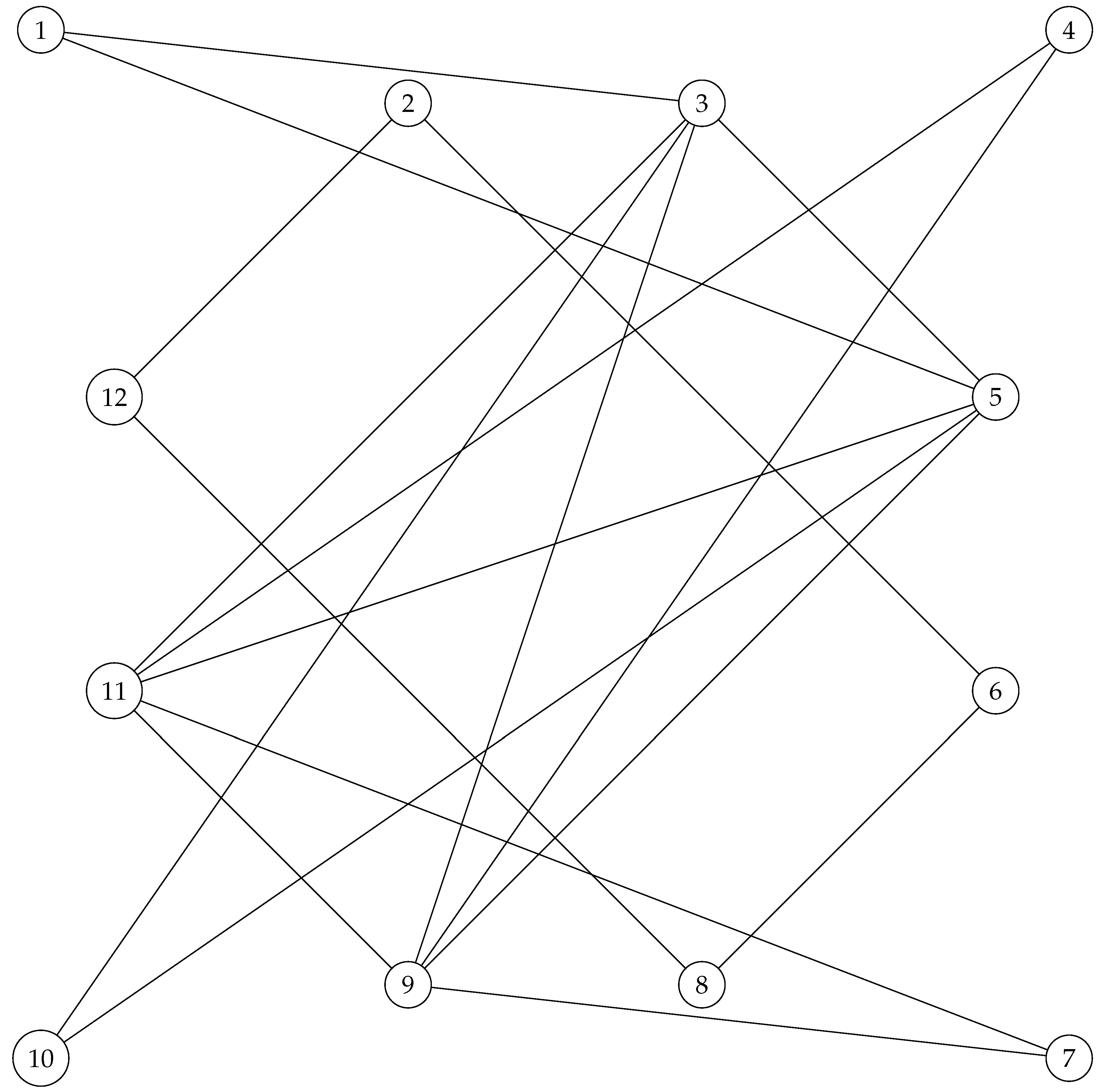
Figure 18.
.
on which its adjacency matrix commutes with the following noncommutative magic unitary matrix
meaning that has quantum symmetries, and the graph ,
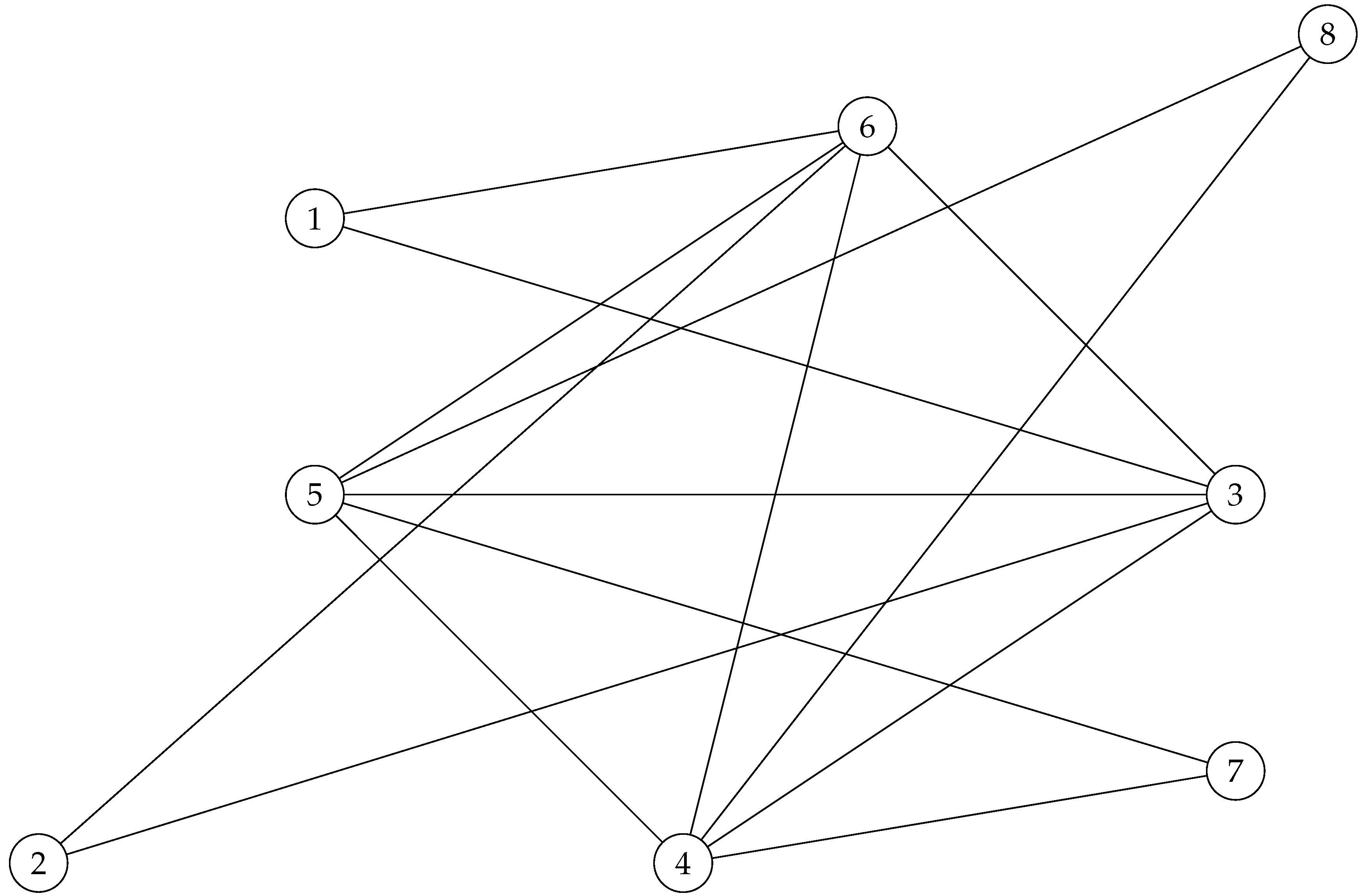
Figure 20.
.
on which its adjacency matrix commutes with the following noncommutative magic unitary matrix
meaning that has quantum symmetries, and as a result, also should has quantum symmetries, and so . It is not too difficult to observe that the only noncommutative commuting magic unitary with , is as follows.
□
Remark 17.
The result obtained in Proposition 3, is already wonderful, but it is not we have been looking for. Because we need a magic unitary consistent with the structures of !
So, consider the graph presented in Figure Section 7.2.2 associated with the following matrix.
Remark 18.
As we mostly are interested in studying the directed graphs with a regulated number of Hamiltonian paths (colored and uncolored versions), hence later on we will see that choosing as in Figure Section 7.2.2 will provide us with the desired result!
Figure 21.
Nine connected graph .
Proposition 4.
has non trivial quantum automorphisms.
Proof.
It is not too difficult to observe that the only noncommutative magic unitary associated with will be as follows for .
This means that has quantum symmetries and the quantum automorphism group is non trivial.
□
Let us try to study , associated with the following matrix in .
Proposition 5.
has non trivial quantum automorphisms.
Proof.
G □
Figure 22.
Eleven connected graph .
7.2.3. Graph algebra structure induced by
Following Remark 16(j), consider the set of graphs . Let be the null graph, a graph with no edges and . Then we have the following definition.
Definition 10.
Let and be as in Remark 16(f, g,h,i). And let and be as above. let be in . Then the connect and overlay operators will be defined as follows for graphs , and .
Lemma 2.
equipped with the connect and overlay operators defined in Definition 10, will be a *-monoid nondegenerate algebra.
Proof.
It is known that any unital algebra is nondegenerate. So the algebra structure equipped on will automatically be nondegenerate. It is not too difficult to see that is closed under the connect and overlay operators defined in Definition 10 and as any graph automatically possesses a * structure, hence one can conclude that equipped with those operators will have a *-monoid algebra structure as s are not invertible! □
Remark 19.
The main point of the Definition 10 and Lemma 2 is that the graphs involved in constructing the *-monoid algebra , have quantum symmetries!
8. The Third Toy Example
In this section we will try to have a reasonable orientation on the set of graphs , that preserves the quantum symmetry!
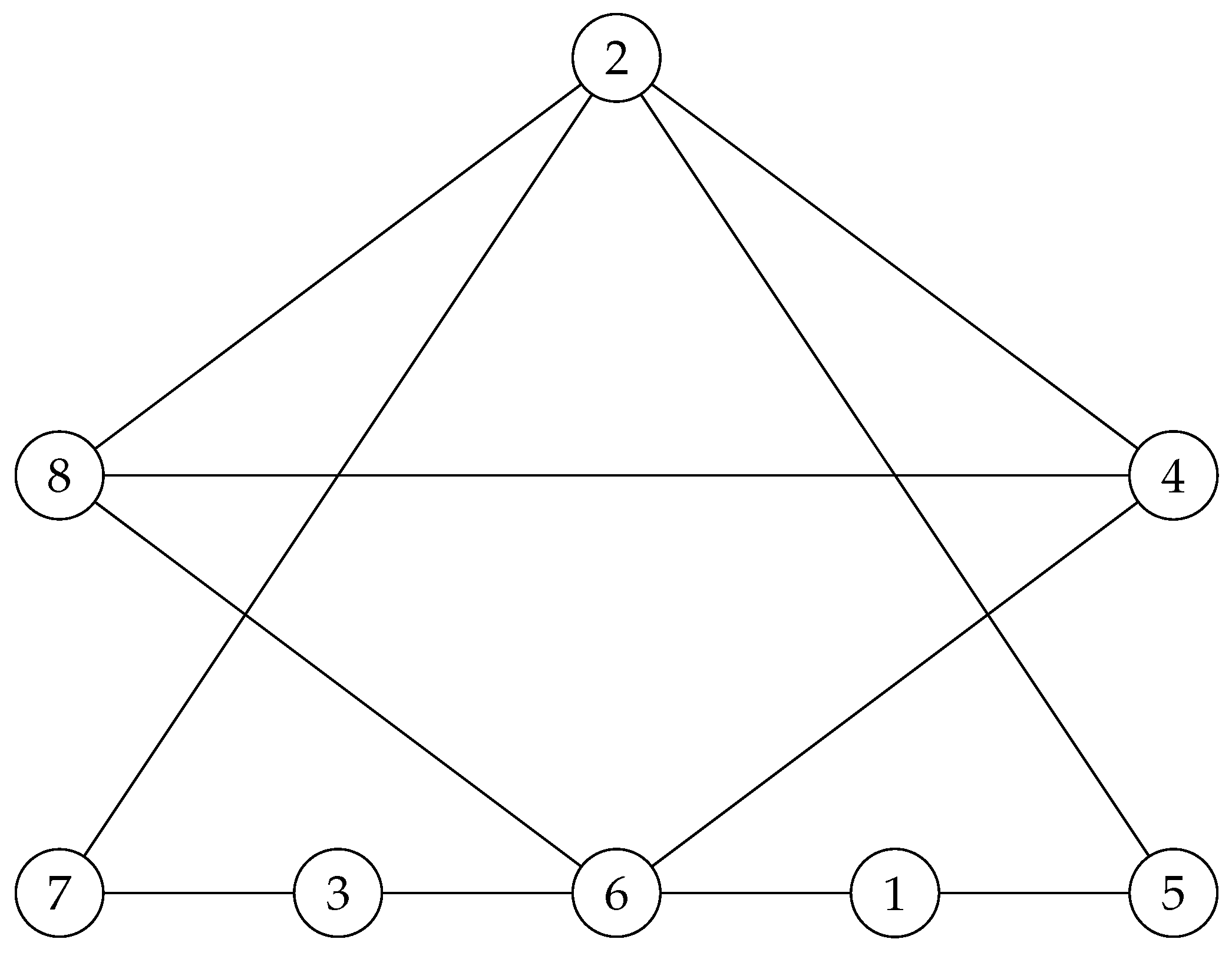
Consider the following oriented graph , which is the oriented version of .
Figure 23.
Totally connected graph .
Note that the adjacency matrix of is , has a unique noncommutative commuting magic unitary
associated with! And hence, possess quantum symmetries and both and should have the same quantum automorphism groups!
Now, let us try to impose the same kind of orientation to and to see how will look like and if it still will have the same quantum automorphism group as in .
Figure 24.
Five connected graph .
And with a rotation , exactly as in the case of , the following graph is obtained.
Figure 25.
Five connected graph .
For some reasons (for instance the not consistent number of Hamiltonian paths) that will become clear later, does not suit our purposes. So, we consider the following graph,
Figure 26.
Totally connected graph .
with the adjacency matrix
Note that interestingly, the graphs presented in Figures Section 8, Section 8 and Section 8 have the same quantum automorphism groups generated by the following noncommutative magic unitary!
Let us try to put a reasonable orientation on in an almost same approach as in , such that has the same automorphism group as in .
One may associate to the following matrix
the directed graph presented in Figure Section 8
Figure 27.
Seven connected graph .
and one gets the following noncommutative magic unitary such that .
But is not following the rules. It is already good, but not what we have been looking for! So consider the following directed graph.
Proposition 6.
has quantum symmetries and its quantum automorphism group is non trivial.
Proof.
Note that one can associate the following adjacency matrix to ,
and it is not too difficult to observe that the only noncommutative magic unitary associated with will be as follows for .
Remark 20.
- i)
- As you may have noticed, we have found a set of regulated graphs, directed and undirected , such that they have the same quantum automorphism groups !
- ii)
- All graphs in and are symmetrizable and quantum symmetrizable!
- iii)
- But the question is why finding such set of graphs is important?
- iv)
- Or better to say, “is it important at all?”
- v)
- The next step is to look for the Hamiltonian paths.
- vi)
- One might also consider the colored version of graphs in and and try to follow the concept introduced in [17]. We will not consider this approach in this paper!
Corollary 5.
- i)
- has 4 Hamiltonian paths.
- ii)
- has 96 Hamiltonian paths.
Proof.
It is not too difficult to observe those Hamiltonian paths starting from vertex 2 or 6, and ending at vertex 4 or 8. We try to omit the complexity here as much as possible! □
Corollary 6.
has Hamiltonian paths for .
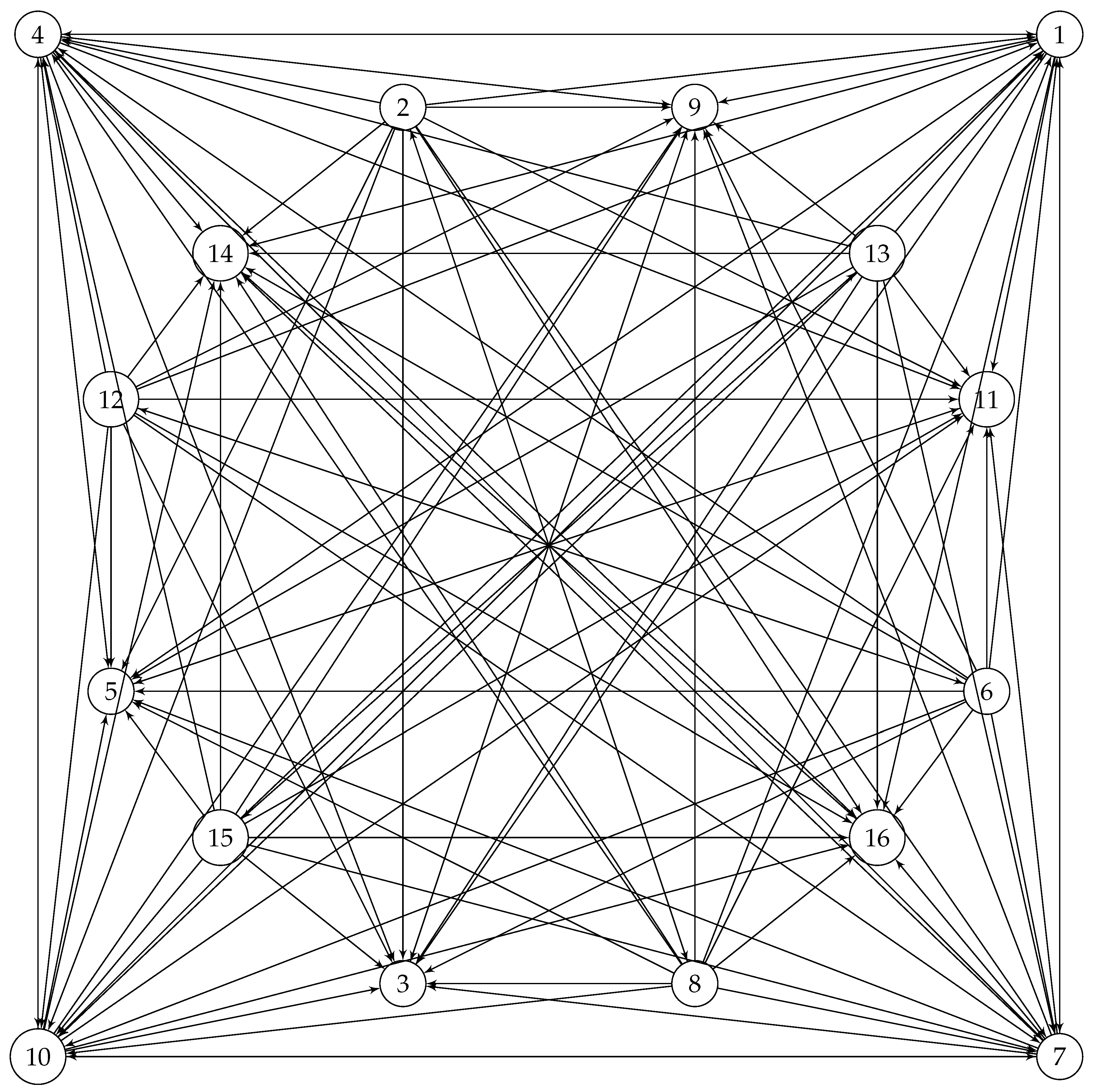
In order to continue, we need to enlarge the class of our directed graphs by having a reasonable orientation on presented in Figure Section 7.2.2 and consistent with the previous orientations. So, let us try to study associated with the following matrix in and presented in Figure Section 8,
Figure 29.
Eleven connected graph .
Proposition 7.
has non trivial quantum automorphisms.
Proof.
It is not too difficult to observe that associated with , we have the following noncommutative projective unitary matrix (magic unitary) that commutes with.
Note that since as the main generators of the quantum automorphism groups of and , respectively, satisfies, hence we get , and they are non-trivial. □
8.1. Graph algebra structure induced by
Before having a graph algebra structure on , we have to present a regulation on the way of defining the orientation on s for . The orientation will follow the one for in [17], with the difference that here we have layers instead of colors. Let and , indicates the sets consisting of source and the sink inner vertices, respectively, and by we will indicate the inner vertices which are neither sink nor source vertices.
Definition 11.
The orientation of the graphs in will be naturally defined as follows
- 1.
- 2.
- 3.
Following subSection 7.2.3, consider the set of directed graphs , and let be the corresponding null graph. Then we have the following definition.
Definition 12.
Let and be as in Definition 11. And let and be as above. let be arbitrary graphs in . Then the connect and the overlay operators will be defined as follows for graphs , and .
Corollary 7.
equipped with the connect and the overlay operators defined in Definition 12, will be a *-monoid nondegenerate algebra.
Proof.
The proof will exactly follow the lines of the proof presented for Lemma 2. □
Remark 21.
- i)
- Note that one may see an undirected graph as a directed graph where each edge has a two sided orientation.
- ii)
- And by using the above vision, one may see as a *-monoid sub-algebra of defined in Definition 10.
9. Quantum Automorphism Groups Associated with and for
In this section, we will use three kind of products between (compact quantum) groups. The semidirect, free, and the (free) Wreath product, which could be explained as follows.
- (I)
- Recall that for compact matrix quantum group , we will refer to as its universal corepresentation. Now consider two compact matrix quantum groups and . Then the compact matrix quantum group of has a structure of a compact matrix quantum group of the form forand the coproduct of will be defined asfor a Woronowicz -subalgebra of both and , with embedings and , respectively, such that and for and the canonical injections and
- (II)
- For G any group, and the direct product of n copies of it, let be an arbitrary permutation. Consider the following action from to .that will constitute the definition of the semidirect product.
- (III)
- For G any group, the Wreath product is a group of the ordered set of tuples with the multiplication defined byfor and , with the identity element .
It is known that every polyhedra has the same symmetry group as its dual. For instance, a cube and an octahedron are dual to each other, meaning that if one puts an octahedron inside a cube, in a natural way such that each vertex of the octahedron sits at the center of one of the cube’s faces, then one can prove that any symmetry of the octahedron corresponds to a symmetry of the cube, and vice versa, and it is equal to the 3-dimensional Hyperoctahedral group (in some literature it is shown by , and in general by ).
The n-dimensional Hyperoctahedral group is isomorphic to the Wreath product of a cyclic group of order 2, with the symmetric group of order n, i.e. , and it has order .
On the other hand we have the Hypercubes. The 1-dimensional Hypercube is the simple line between 2 points, and its symmetric group is which is the 1-dimensional Hyperoctahedral group. The 2-dimensional Hypercube is a square, and its symmetric group is , which is the 2-dimensional Hyperoctahedral group . The 3-dimensional Hypercube is the 3-dimensional cube, and its symmetric group is , which is the 3-dimensional Hyperoctahedral group . The 4-dimensional Hypercube is a 4-dimensional cube, known as the Tesseract, and its symmetric group is , which is the 4-dimensional Hyperoctahedral group , and so on!
Remark 22.
Here in this paper, our concern will be more about the and 4-dimensional Hyperoctahedral groups and their quantum versions. But our results could be generalized to the higher dimensions as well!
9.1. The quantum Hyperoctahedral groups and their relations with and for
As we mentioned in the introduction, following Wang’s definition of quantum permutation group of a set [22], satisfying the formalism of Woronowicz’s compact quantum group [23], Banica came with an idea [3], while improving the previously formulated structures of the quantum automorphism group of a graph [5], but presenting much efficient structure by using the projective permutation matrices, known as magic unitaries in quantum group literature, by considering the commutative algebra of complex-valued functions on the automorphism group of a graph, and then by dropping the commutativity requirement of the generators in order to get the algebra of continuous functions on the quantum automorphism group of the given graph!
In order to avoid the complexity, the quantum automorphism groups of many classes of undirected graphs have have already been studied, from which, we can mention the n-cycle graphs (), the complete graphs , the Petersen graph, Hyper cubes, the Odd graphs, Hamming graphs , the Johnson graphs , the Kneser graphs , the Moore graphs of dimension two, the Paley graphs [18,20].
However, for the cycle graph , Bichon in [5], proved that its quantum automorphism group is isomorphic with the quantum dihedral group. Later on, in [6], he provided a proof showing that the n-dimensional hyperoctahedral group, as the isometry group of a hypercube in , is the Wreath product .
In [21], Schmidt and Weber showed that the Hyperoctahedral quantum group is the quantum automorphism group of the 4-cycle , meaning that
In [1], concerning the quantum automorphism group of the disjoint union of graphs (directed and undirected), the authors provided a very nice classification, from which one could determine the quantum automorphism of disjoint union of any finite set of connected simple graphs, and it could be simplified as follows.
- i)
- For a disjoint union of n-pairwise non-quantum isomorphic connected graphs , the quantum automorphism group of the union will be given by the free product of the quantum automorphism group of the individual graphs , i.e.
- ii)
- For a disjoint union of n isomorphic copies of a connected simple graph , the quantum automorphism group of the union will be given by the free Wreath product of the quantum automorphism group of by the quantum permutation group , i.e.
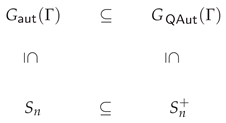
As it is apparent from the title of the current section, this section concerns with the quantum automorphism group of the undirected graphs and their oriented versions , for . But as the group of quantum automorphisms of an arbitrary graph is an infinite dimensional compact matrix quantum group generated by certain projective permutation matrices (magic unitaries), and as in our case, the generators of coincide with the generators of , hence we should have .
Remark 23.
- i)
- Note that, for Γ an arbitrary graph, here we follow the definition of quantum automorphism group of Γ proposed by Banica [3], and we call it .
- ii)
- As and are isomorphic with the complete graphs and , respectively, and it is known that the quantum automorphism group of and are and [22], respectively, hence we have
Lemma 3.
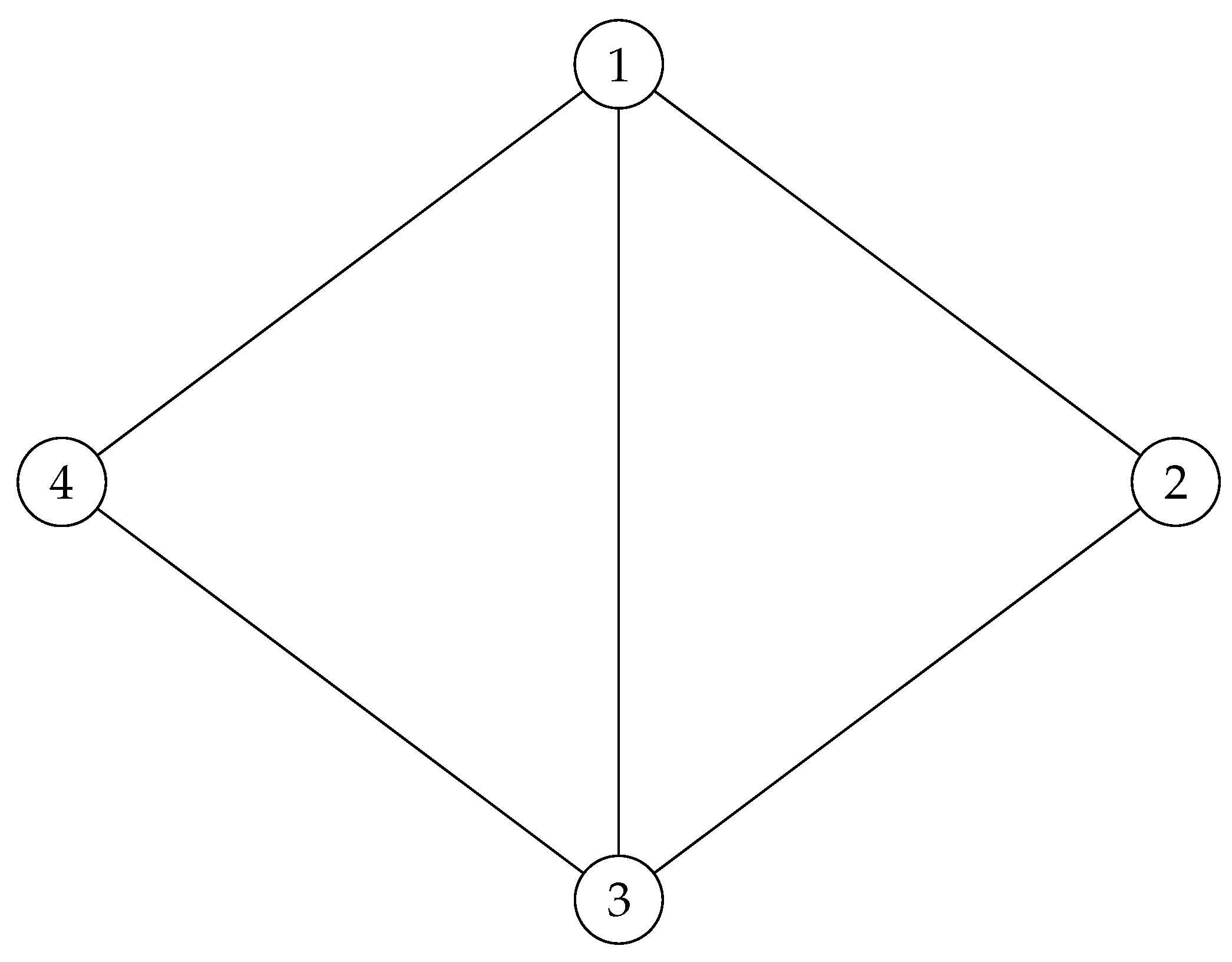
The regular tetrahedron has nontrivial quantum automorphisms.
Proof.
In order to prove that the regular tetrahedron possesses quantum symmetries, first we try to give it a reasonable orientation as follows.
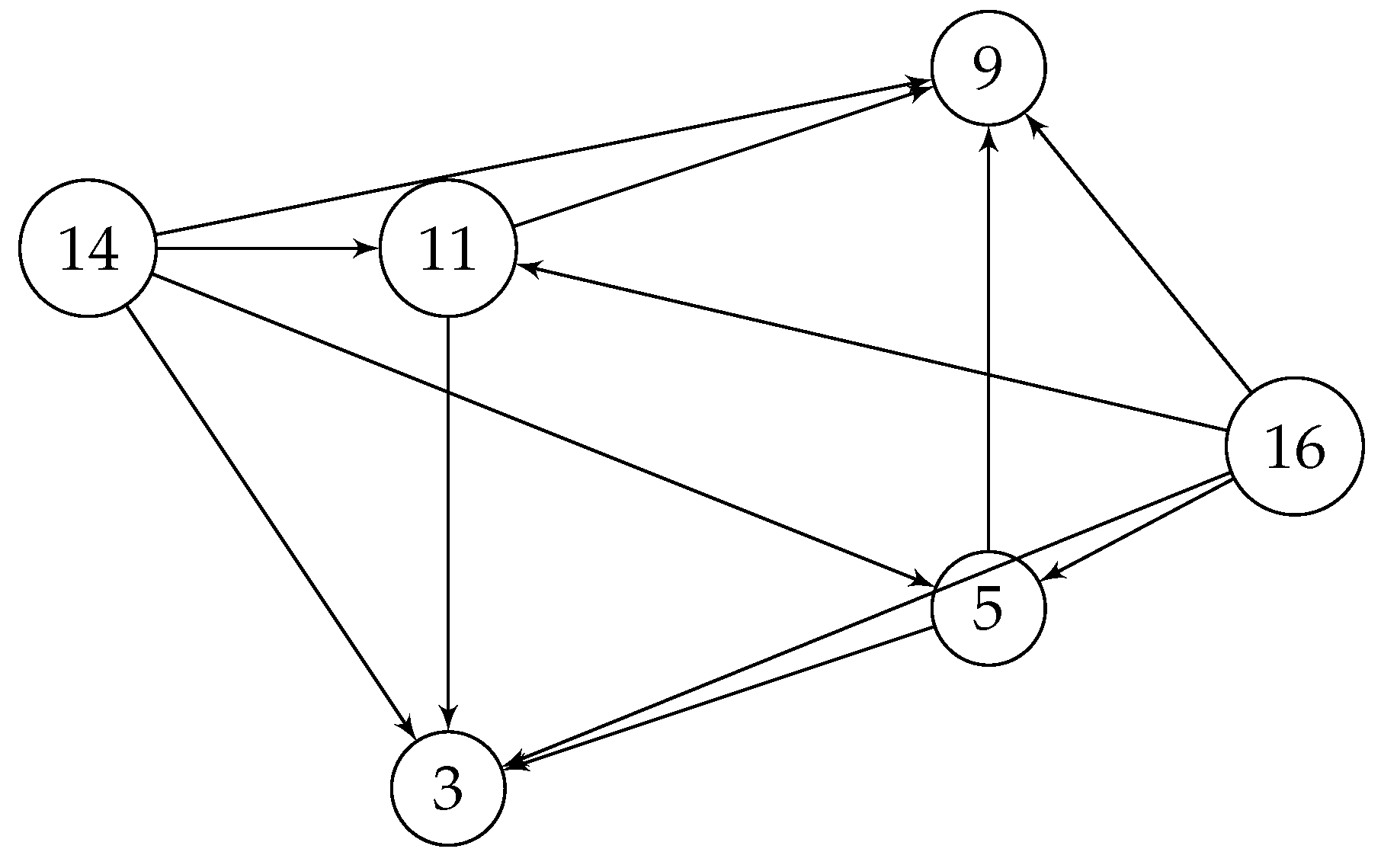
Figure 30.
.
Note that to presented in Figure Section 9.1, one can associate the following adjacency matrix,
and it is not too difficult to see that the following noncommutative magic unitary (projective unitary matrix) commutes with .
i.e. , and has non-trivial quantum symmetries.
However, one may as well tries to clarify that also commutes with the adjacency matrix
associated with the undirected regular tetrahedron, meaning that satisfies and has non-trivial quantum automorphisms, and this concludes the proof.
□
Corollary 8.
The group generated by the projective unitary matrices , for mutually noncommutative entries (they could be any kind of matrices in for , with the same living space), is isomorphic to the 3-dimensional quantum hyperoctahedral group
Figure 31.
.
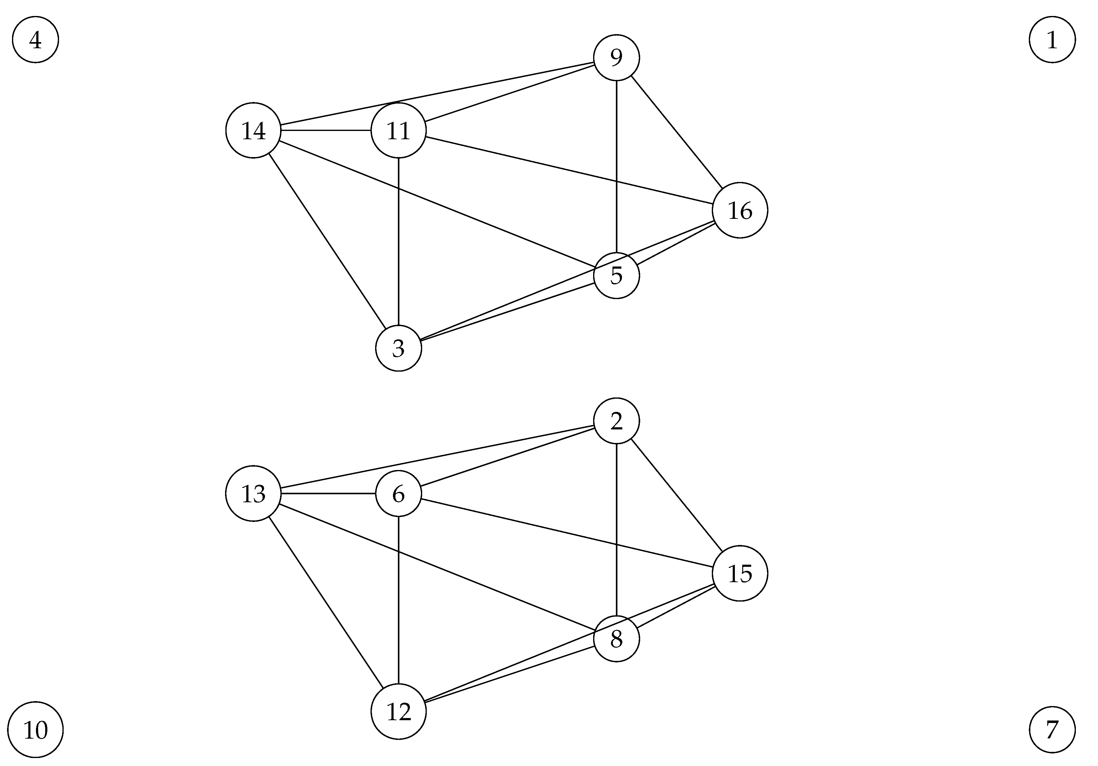
Figure 32.
.
Proposition 8.
The quantum automorphism groups of and are non-trivial and are equal to
Proof.
From Lemma 1, we already know that for . Hence what we need is just to compute the quantum automorphism group of , and by using the classification criteria mentioned in b and a, and the fact that the quantum automorphism group of the null graph in 4 vertices is , by following Figures Section 7.2.2 and Section 9.1 one would get the desired results. □
Lemma 4.
The quantum automorphism group of for is non-trivial and is equal to
Proof.
It is a direct consequence of Proposition 8 and the fact that for . □
Corollary 9.
The quantum automorphism group of for is non-trivial and is equal to
10. Concluding Remarks
Now the question is what might be the main implications of the above statements and results?
One would be finding a path into the generalized Cartan matrices, and the Kac-Moody algebras, and to see how the results obtained and studied in the Section 7 could be generalized into the theory of quantum groups!
On the other hand, the process used in Example 9 triggered mathematicians to come up with the idea of the metric isometry game [12], for metric spaces X and Y as a modification of the graph isomorphism game , which is a game introduced by Atserias et al [2], with the property that two graphs and are isomorphic if and only if there exists a perfect deterministic strategy for . These kind of structures are a part of the so called non-local game, which is a game played cooperatively by two players called Alice and Bob. However, following the discussion part of [13], and the result obtained in Lemma 4, one might be interested in asking if it is possible to construct a non-classical perfect quantum strategy for the -isomorphism game (referred to as the -automorphism game), for ? (We have to admit that this is not an easy direction to consider!)
But, about the results obtained in this paper, we have to emphasize that still there are many things to do. We still haven’t been able to study the colored version of the graphs which could be very interesting as this set of graphs is quite different from the ones studied in [15,16,17], as these graphs possess quantum symmetries and their quantum automorphism groups is non-trivial.
One may also try to study the *-monoid algebra structure on the set of directed graphs .
Funding
This research was in part supported by a grant from IPM (No. 1404140052)
Acknowledgments
The author is partially supported by a grant from the Institute for Research in Fundamental Sciences (IPM), with grant No. 1404140052.
References
- Árnadóttir, Árnbjörg Soffía, Josse van Dobben de Bruyn, Prem Nigam Kar, David E. Roberson, and Peter Zeman. Quantum Sabidussi’s Theorem. arXiv 2024, arXiv:2402.12344.
- S. A. Atserias, L. Mančinska, D. Roberson, R. Samal, S. Severini, and A. Varvitsiotis. Quantum and non-signalling graph isomorphisms. Journal of Combinatorial Theory 2019, 136, 289–328. [Google Scholar]
- Banica, T. Quantum automorphism groups of homogeneous graphs. Journal of Functional Analysis 2005, 224, 243–280. [Google Scholar] [CrossRef]
- Julien Bichon, An De Rijdt, and Stefaan Vaes. Ergodic coactions with large multiplicity and monoidal equivalence of quantum groups. Communications in Mathematical Physics 2005, 262, 703–728. [Google Scholar] [CrossRef]
- Julien Bichon. Quantum automorphism groups of finite graphs. Proceedings of the American Mathematical Society 2003, 131, 665–673. [Google Scholar]
- Julien Bichon. Free wreath product by the quantum permutation group. Algebr. Represent. Theory 2004, 7, 343–362. [Google Scholar] [CrossRef]
- Carter, R.W. , Lie algebras of finite and affine type, Cambridge Studies in Advanced Mathematics 96, Cambridge University Press, Cambridge 2005.
- McKee, James, and Chris Smyth. Symmetrizable matrices, quotients, and the trace problem. Linear Algebra and its Applications 2020, 600, 60–81. [Google Scholar] [CrossRef]
- Nechita, I.; Schmidt, S.; Weber, M. Sinkhorn algorithm for quantum permutation groups. Experimental Mathematics 2023, 32, 156–168. [Google Scholar] [CrossRef]
- Eifler, Kari. Non-local games and quantum symmetries of quantum metric spaces. arXiv 2020, arXiv:2011.03867. [Google Scholar] [CrossRef]
- JUNK, Luca Leon. Quantum Automorphism Groups of Graphs and Coherent Algebras. PhD diss., Saarland University,.
- Eifler, Kari. Quantum Symmetries Studied through the Lens of Non-local Games. PhD diss., Texas A&M University.
- M. Lupini, L. Mančinska, and D. Roberson. Nonlocal games and quantum permutation groups. Journal of Functional Analysis 2017, 12. [Google Scholar]
- Razavinia, Farrokh, and Haghighatdoost, Ghorbanali. From Quantum Automorphism of (Directed) Graphs to the Associated Multiplier Hopf Algebras. Mathematics 2024, 12, 128. [Google Scholar]
- Razavinia, Farrokh. Into Multiplier Hopf (*-)graph algebras. arXiv, arXiv:2403.09787.
- Razavinia, Farrokh. A route to quantum computing through the theory of quantum graphs. arXiv 2024, arXiv:2404.13773. [Google Scholar] [CrossRef]
- Razavinia, Farrokh. C*-Colored graph algebras. arXiv 2025, arXiv:2504.16963.
- Schanz, Julien. Quantum symmetries of vertex-transitive graphs on 12 vertices. Journal of Noncommutative Geometry.
- Simon Schmidt, Quantum automorphisms of folded cube graphs. Annales de lInstitut Fourier 2020, 70, 949–970. [CrossRef]
- Schmidt, Simon. Quantum automorphism groups of finite graphs. PhD diss., Saarland University, 2020.
- Schmidt, Simon, and Moritz Weber. Quantum symmetries of graph C*-algebras. Canadian Mathematical Bulletin 2018, 61, 848–864. [Google Scholar] [CrossRef]
- Shuzhou Wang. Quantum symmetry groups of finite spaces. Communications in Mathematical Physics 1998, 1, 195–211. [Google Scholar] [CrossRef]
- Stanislaw, L. Woronowicz. Compact matrix pseudogroups. Communications in Mathematical Physics. 1987, 111, 613–665. [Google Scholar]
Disclaimer/Publisher’s Note: The statements, opinions and data contained in all publications are solely those of the individual author(s) and contributor(s) and not of MDPI and/or the editor(s). MDPI and/or the editor(s) disclaim responsibility for any injury to people or property resulting from any ideas, methods, instructions or products referred to in the content. |
© 2025 by the authors. Licensee MDPI, Basel, Switzerland. This article is an open access article distributed under the terms and conditions of the Creative Commons Attribution (CC BY) license (http://creativecommons.org/licenses/by/4.0/).
Copyright: This open access article is published under a Creative Commons CC BY 4.0 license, which permit the free download, distribution, and reuse, provided that the author and preprint are cited in any reuse.


