Submitted:
29 August 2025
Posted:
03 September 2025
You are already at the latest version
Abstract
In the context of a medical imaging application for preclinical research, specifically, erebrovascular imaging in small animals, this work examines the challenges of using a Large-Scale 2D ultrasonic array with 32×32 elements (96×96 wavelengths). The application imposes demanding requirements: very near-field operation, high spatial resolution, high frequency, high frame rate, and imaging in a highly attenuating medium. These needs, combined with current technological limitations, such as element size and constraints on the number of elements that can be driven in parallel, pose significant challenges for system design and implementation. To evaluate system performance, we use plane wave imaging as a reference mode due to its ability to meet high acquisition speed requirements. Our analysis highlights limitations in spatial coverage and image quality when operating the full aperture under planewave transmission constraints. To overcome these limitations, we propose a sparse aperture strategy. When integrated with advanced signal processing techniques, this approach improves both contrast and resolution while maintaining acquisition speed. This makes it a promising solution for high-performance ultrasonic imaging under the demanding conditions of preclinical research.
Keywords:
ultrasonic imaging
; bidimensional aperture
; ultrafast imaging
; beamforming
1. Introduction
Ultrasound imaging has become an essential tool in preclinical cerebrovascular research due to its ability to provide non-invasive, real-time, and high-resolution visualization of cerebral anatomy and hemodynamics [1,2]. This modality enables the assessment of cerebral blood flow, tissue perfusion, and blood-brain barrier integrity in animal models, thereby facilitating the investigation of conditions such as ischemic stroke, cerebral hemorrhage, and small vessel disease [3]. The use of contrast agents enhances sensitivity for detecting microvascular alterations and changes in vascular permeability. Additionally, its affordability and portability support longitudinal studies without the need for repeated invasive procedures. Ultrasound is also employed to monitor therapeutic responses, including neuroprotective agents and reperfusion strategies. When integrated with other imaging modalities such as magnetic resonance imaging (MRI) or positron emission tomography (PET) [4], it enables multimodal analysis, offering a versatile and efficient platform for advancing the understanding of cerebrovascular pathophysiology and the development of novel therapeutic approaches[1,2,5].
Despite these advantages, the implementation of high-frequency and volumetric ultrasound imaging using 2D arrays in animal research presents several technical challenges [6,7,8]. Although frequencies above 15 MHz improve spatial resolution, they remain insufficient for visualizing deep or small-caliber vascular structures, particularly in rodent brains. Anatomical access is further constrained by the skull, which attenuates ultrasound waves and degrades image quality, often necessitating craniotomies or the use of acoustic windows [10]. Volumetric imaging with 2D arrays enables three-dimensional reconstruction of vascular flow and morphology but is highly susceptible to motion artifacts—such as respiration and cardiac pulsation—that complicate stable data acquisition. Moreover, the limited penetration depth of high-frequency waves restricts imaging to superficial cortical regions, excluding deeper structures. These limitations underscore the need for optimized imaging protocols, specialized transducer designs, and advanced compensation strategies to improve image quality and utility in preclinical cerebrovascular studies [6,9,10,11].
Ultrasonic plane-wave imaging plays a key role in cerebrovascular imaging by enabling ultra-fast acquisitions that capture cerebral blood flow dynamics with high temporal resolutionite [12]. Although this method can produce an image with just one shot, it tends to produce significant sidelobes and reduced image quality compared to focused beam techniques, these artifacts can be mitigated by compounding multiple images acquired at different transmission angles, thereby enhancing overall image fidelity. This technique facilitates the visualization of small vessels and improves image quality by compounding multiple transmission angles, making it ideal for both functional and structural brain studies in preclinical and clinical settings. In linear arrays, typical angle sets range from 3 to 30, while 2D arrays commonly use configurations spanning from to angles. Determining the optimal number of transmission angles requires experimental validation or simulation to strike a balance between image quality and acquisition complexity [7,10,13].
In this context, volumetric imaging remains a technological challenge, particularly in achieving apertures large enough to ensure high resolution. At high frequencies, the constraint of maintaining half-wavelength element spacing to avoid grating lobes is incompatible with the need to transmit sufficient energy into the medium or to ensure adequate sensitivity of each element, and can lead to a number of parallel channels too high for current electronic devices. For this reason, supported by the plane-wave imaging modality, there is a growing trend toward the development of transducers with larger elements [9]. Most research results are based on Large-Scale 2D ultrasonic array (, BW=70%) with inter-element spacing of approximately , as this represents the largest commercially available aperture (Vermon S.A.). However, due to the size of the elements, these systems have limited capabilities and are complex to operate. Moreover, controlling such a large number of elements in parallel is technically demanding. Only recently have systems emerged capable of managing up to 256 channels simultaneously, often relying on complex multi-system configurations. The quality of plane-wave imaging depends on diversity: combining images with varying beam profiles enhances reflector visibility and suppresses sidelobes, especially within the aperture’s projection zone.
This work explores how to implement a volumetric imaging system using such apertures while operating with a reduced number of active elements for preclinical imaging in small animal models. Specifically, based on the array with element spacing, we propose a solution for 256 active elements capable of generating plane-wave images with a reduced number of acquisitions with regard to sequentialy multiplexing the active aperture along the whole array.
2. Materials and Methods
The intended application focuses on the study of stroke and aims to develop analytical tools for tissue characterization, anatomical element identification, and cerebrovascular system analysis in rats (see Figure 1). The project is currently in an early stage, prior to experimental work, where we are defining the instrumentation, its operability, and the adaptation requirements for the application.
The rat brain has an approximate volume of , with a length ranging from 2 to 2.5 cm and a depth between 1 and 1.5 cm. From an ultrasound perspective, it presents several challenges: high-frequency imaging is required, the tissue is highly attenuating, and the skull acts as a difficult-to-penetrate barrier [14]. In this context, it is important for the sensor to be positioned as close as possible to the region of interest in order to minimize the impact of attenuation. However, this may cause the transducer to operate in a region where it is not efficient. Additionally, there are practical difficulties associated with working with small animals. Although several studies focus on this type of application and provide details on positioning and coupling mechanisms, few describe the operability of the array. In anatomical imaging mode, it delivers limited image quality, and a large volume of images along with complex post-processing is needed to produce accurate representations of the cerebrovascular structure.
In our case, we propose working with the SITAU II ultrasound imaging system (DASEL SISTEMAS S.L.), capable of operating with 256 channels and a two-dimensional aperture of 15 MHz, consisting of elements and a lateral size of 96 wavelengths (BW 70%). The aim of this work is to develop an analysis of the aperture’s performance to determine its application range, and to adapt it to a total of 256 active elements by designing the multiplexing system and its operability.
This work is carried out in a theoretical setting and based on simulation models. For this purpose, custom computational models have been developed, based on the simulation framework proposed by Piwakowski [15].
3. Large-Scale 2D array
In a 2D array configuration, the use of conventional elements sized at presents significant challenges, even in the relatively straightforward case of a full matrix array. Beyond the need to balance performance with hardware limitations (reducing the number of elements), the design process must also address trade-offs between the intrinsic capabilities of the aperture and the specific application requirements—such as penetration depth, beam steering, spatial resolution, dynamic range, and element sensitivity.
In this context, a matrix array employing elements sized at (see Figure 2-A) clearly prioritizes radiation efficiency and sensitivity over beam steering capability. This configuration, compared to half-lambda elements, yields a increase in both radiation efficiency and sensitivity. However, this enhancement introduces a diffraction-induced modulation in the array response, resulting in a sensitivity drop of approximately at an angle of , thereby limiting the array’s steering range. Figure 2-B illustrates the focal behavior at various steering angles and highlights the associated reduction in dynamic range.
This design choice becomes evident when considering the attenuation characteristics of the inspection scenario. At , the acoustic attenuation within the biological tissue is approximately . Additionally, the use of a coupling medium introduces further attenuation of around . Consequently, maximizing the transmitted energy into the biological tissue is critical, and minimizing the propagation path through theion coupling layer is advantageous. Figure 2-C shows the impact of attenuation on the acoustic field along the propagation axis for the biological tissue and for the coupling layer. From this point, the attenuation effect of the coupling medium will be included in all simulations.
3.1. Plane-wave generation
Given that another requirement of the application is to achieve high acquisition speed, we evaluated the performance of the full aperture for Plane-wave transmission within this depth range. In Figure 3, we present the beampattern of several cases of planar aperture steering (cases of , , and , see Figure 3A, Figure 3B, and Figure 3D), and we show the cross-section at for steering angles from to .
The first observation is that the acoustic field exhibits a ripple of approximately in all cases. Moreover, as the steering angle increases, the field amplitude not only decreases compared to the case, but a lobe platform also emerges at approximately , which facilitates the appearance of imaging artifacts caused by out-of-focus reflectors. For example, at , a loss of in the main lobe is observed, along with the formation of a side lobe structure only below, potentially introducing artifacts into the image.
Therefore, the beam steering capability is significantly limited. The diversity of the plane wave is constrained to a range between and , with a reduction in the overlap region, and consequently in imaging performance, to approximately to .
3.2. Aperture performance
Given the proximity between the imaging region and the array, and the limited beam steering capability of the elements, we evaluated individual element contribution to the image by analyzing the intensity with which each element perceives every point within the region of interest. For efficient focusing and optimal aperture utilization, it is desirable that the intensity contribution from each element at a given point in space be of a similar order of magnitude.
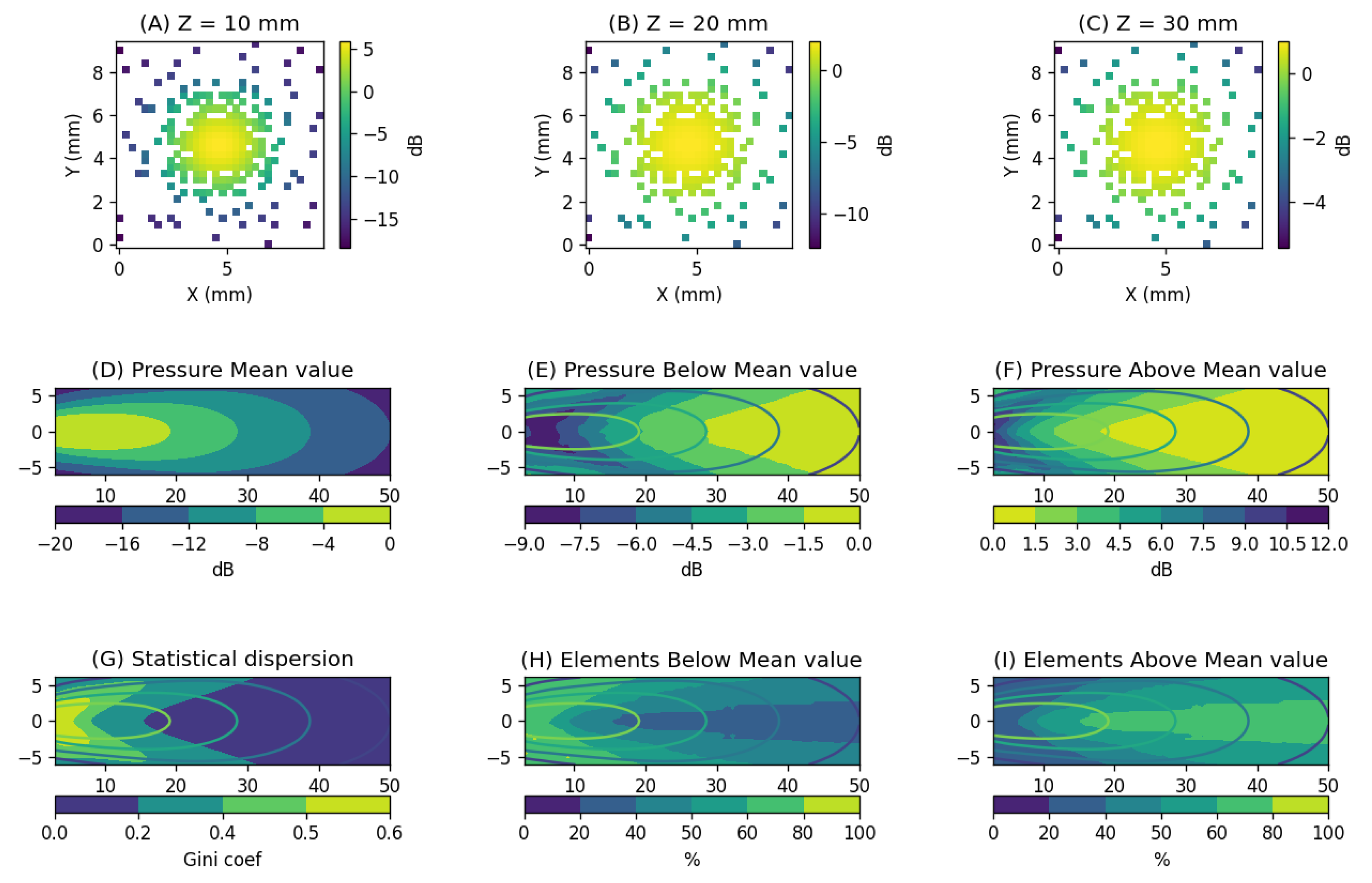
In this study, for each point in the region of interest, we computed the influence of 1024 elements and analyzed how these values are distributed relative to their mean. As an example, we show the distribution of these values—normalized to their mean—at three specific axial positions: (Figure 4-A), (Figure 4-B), and (Figure 4-C). It can be observed that at shallow depths, the differences are quite significant, compromising the efficient use of the associated electronic resources for certain elements. As depth increases, the intensity distribution becomes more uniform, improving the operational balance of the imaging system.
The Figure 4-D shows the average intensity level across the elements, highlighting that maximum participation occurs between and . These curves will be included as reference overlays in all spatial plots. Figure 4-E and Figure 4-F illustrate the distribution of values below and above the mean, respectively. Notably, in the region of maximum average intensity, differences of up to between extreme values can be observed.
Additionally, we evaluated the percentage of the aperture that contributes above and below the mean intensity level (Figure 4-H and Figure 4-I, respectively). The requirement for a balanced aperture allowed operation from depths starting at . However, as observed in Figure 4-E and Figure 4-F, this condition may still result in intensity differences of up to , introducing a natural apodization effect across the aperture.
Finally, to assess the degree of similarity among the elements, we used the Gini coefficient [16,17]. This metric quantifies the level of inequality within a set of values and is particularly useful for analyzing distributions with significant internal variation, as is the case here. Values close to zero indicate high similarity, while values near one reflect high inequality (Figure 4-G).
Values below indicate low inequality; values between and indicate moderate inequality; and values above imply high inequality.
The Gini plot shows that below , the acoustic field is mainly determined by a small number of elements, resulting in low resource utilization. For full aperture, a compromise solution can be found starting from .
From the simulations, we can deduce that the optimal scanning range capable of covering the full aperture can be approximated as a cylinder from to with a diameter of . In this case, the pulse-echo attenuation is approximately , and if we consider shifting the scanning zone by (from to ), the attenuation increases to .
4. Sparse aperture
After defining the working conditions for the full aperture in the region of interest and identifying the steering limitations of plane-wave emissions, strategies can be proposed to reduce the number of active elements, thereby optimizing the use of the aperture’s performance. Diversity is introduced by sparsifying the aperture, employing distinct sparse configurations that preserve coincident reflector responses while generating different sidelobe patterns, thus enhancing imaging diversity. This approach enables a single emission to uniformly cover the entire region of interest with balanced intensity.
The objective is therefore not to determine a unique optimal aperture, but rather to define a set of apertures that share common beampattern characteristics and, when combined with random generation, provide the required diversity. To this end, the aperture is partitioned into bins, and different apodization schemes are applied in both transmission and reception as a function of the intended behavior within the binned array structure [7]. Figure 5 illustrates three of the designed strategies.
In this approach, each aperture is defined as an bin structure (with elements per bin), where the window specifies the number of elements to be activated in each bin according to its intensity. Within each bin, the active elements are selected randomly.
4.1. Sparse Emission Aperture. Inner Region
The goal of the transmission is to ensure uniform insonification of the region of interest while enabling rapid energy dispersion outside this region, thereby minimizing the influence of external noise sources on the image. The wavefront should remain planar, temporally narrow, and to span the widest possible coverage area, free from secondary fronts that could degrade the dynamic range. Accordingly, we aim for an aperture capable of generating a wide, flat beam with low sidelobes. This can be achieved through aggressive windowing that reduces the contribution of the outer elements.
This window must be adapted to the available resources [8,19]. In addition to the spatial discretization already employed (a matrix grid with spacing of ), we consider the limitation that the emission amplitude cannot be controlled and is assumed to be fixed for all elements. Consequently, the windowing effect is achieved by adjusting the density of active elements within each bin (see Figure 5).
Ultimately, the resulting aperture should be regarded not as an exact realization of the theoretical model, but as a practical approximation. In Figure 6, we show an example comparing the desired apodization (a Taylor window) with the one actually achieved. The resulting shape is significantly distorted due to the grid structure, which favors alignment in the projection of the elements. The contrast in the obtained field is 10 times higher than desired, although both patterns match along the axis within a range of (see Figure 6(B)).
An aperture designed with a Taylor window was analyzed, and the contribution of its elements to insonifying the region of interest was evaluated. Balanced participation occurs at depths beyond 10 mm. Although edge and outer elements show lower participation, especially near the aperture, the number of channels with above-average intensity exceeds those with low intensity. This behavior remains consistent with the intended apodization.
Figure 6.
This figure illustrates the difference between the desired acoustic field for the transmitting aperture and the field that can actually be achieved given the technical limitations. Specifically, the elements are arranged in a grid, and each can only be activated or deactivated. Figure (A) shows the ideal field. Figure (C) presents the apodization, represented over the equivalent linear array at axis X=0, achieved with a binarized aperture, where elements within each bin are randomly selected. Figure (B) displays both the desired field (blue line) and the achieved field (orange line). Figure (D) shows the achieved field again for further analysis.
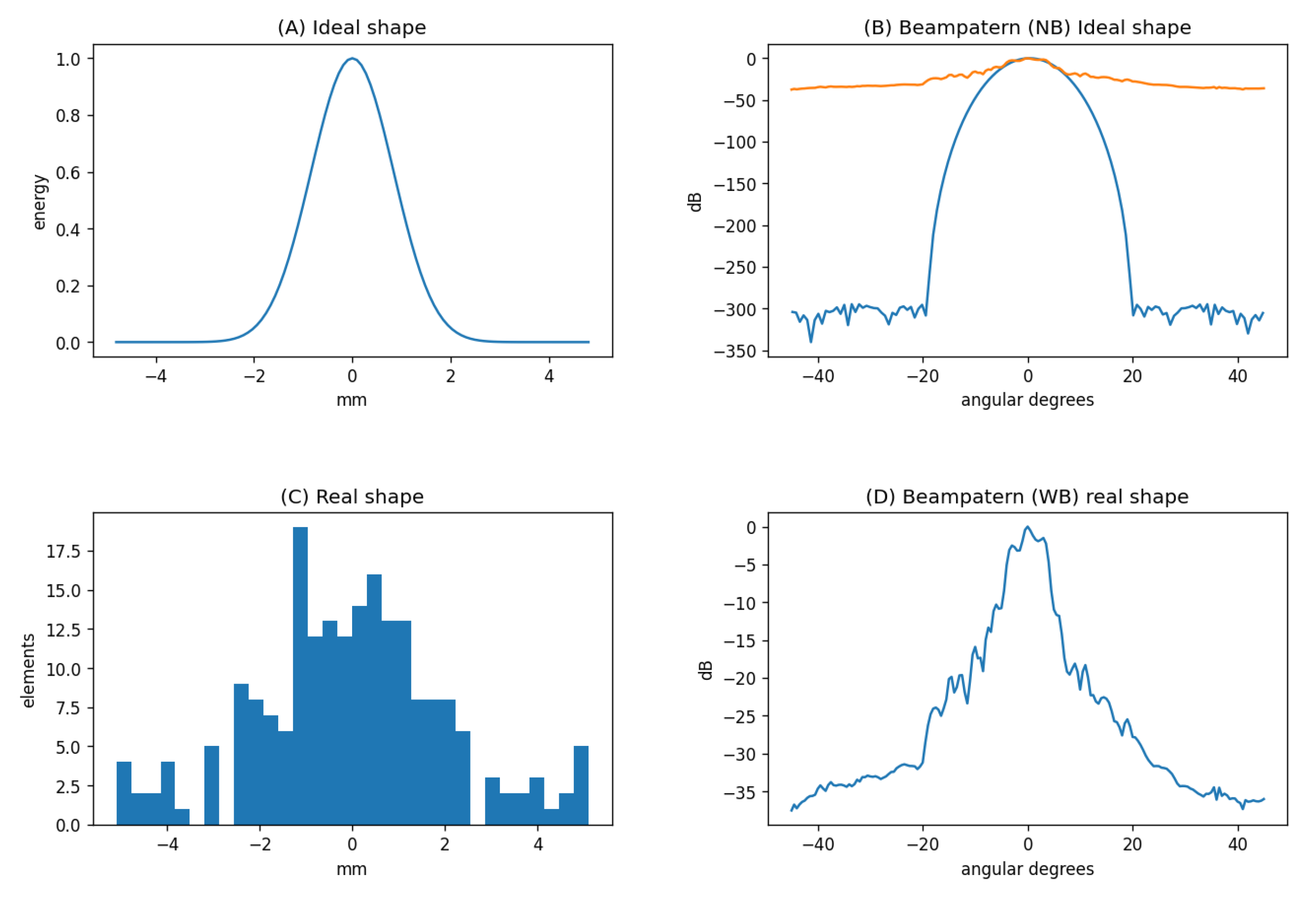
Figure 7.
For the Taylor apodized aperture analysis at different points in space, we considered the region and . Figures A–C show the amplitude with which the aperture elements influence three points along the axis at depths of (A) , (B) , and (C) . Taking the mean value as a reference, we observe differences ranging from up to 20 dB in (A) to around 6 dB in (C). Figure D shows the average gain level exerted at each point in the plane. The values in (E) represent the level reached by elements below the mean, while (F) shows the values above it. In (G), we present the statistical dispersion of these values, calculated using the Gini coefficient. Figure (H) displays the percentage of elements below the mean, and Figure (I) shows the percentage above the mean.
If we observe the acoustic field generated between and , in another particular case of this strategy, we see that it has an irregular structure. (see Fig Figure 8 However, it drops rapidly—by nearly 25 dB—for X values close to . The distribution of secondary lobes is highly irregular, and as in the case of the full aperture, deflection severely penalizes the dynamic range. It is not possible to go beyond , preventing efficient overlap between deflected images.
The defined strategie allows the generation of different apertures for a given apodization, resulting in similar main-lobe behavior but varying side-lobe distributions. For this same strategy, we can compare the performance of several apertures in Figure 9. For each of them, the field has been calculated at (from to ) under flat emission, and the shape of their wavefronts has been obtained. Both the similarities and differences among these images are of interest for this application.
The usable imaging area is limited to a region of , where the apertures still show small differences, and the behavior of the tails of the wavefront varies in each case. The goal is to leverage the technical limitations that prevent perfect apodization as a tool to generate diversity.
To introduce diversity in the signals and exploit it, the reception aperture must be fixed. In this case, a series of consecutive transmissions can be averaged if received through the same reception aperture—even directly within the acquisition system. If the transmission aperture is fixed, this averaging reduces the system’s electronic noise only, thereby improving contrast. However, if the transmission aperture varies from shot to shot, part of the acoustic noise it generates can also be mitigated, further enhancing contrast
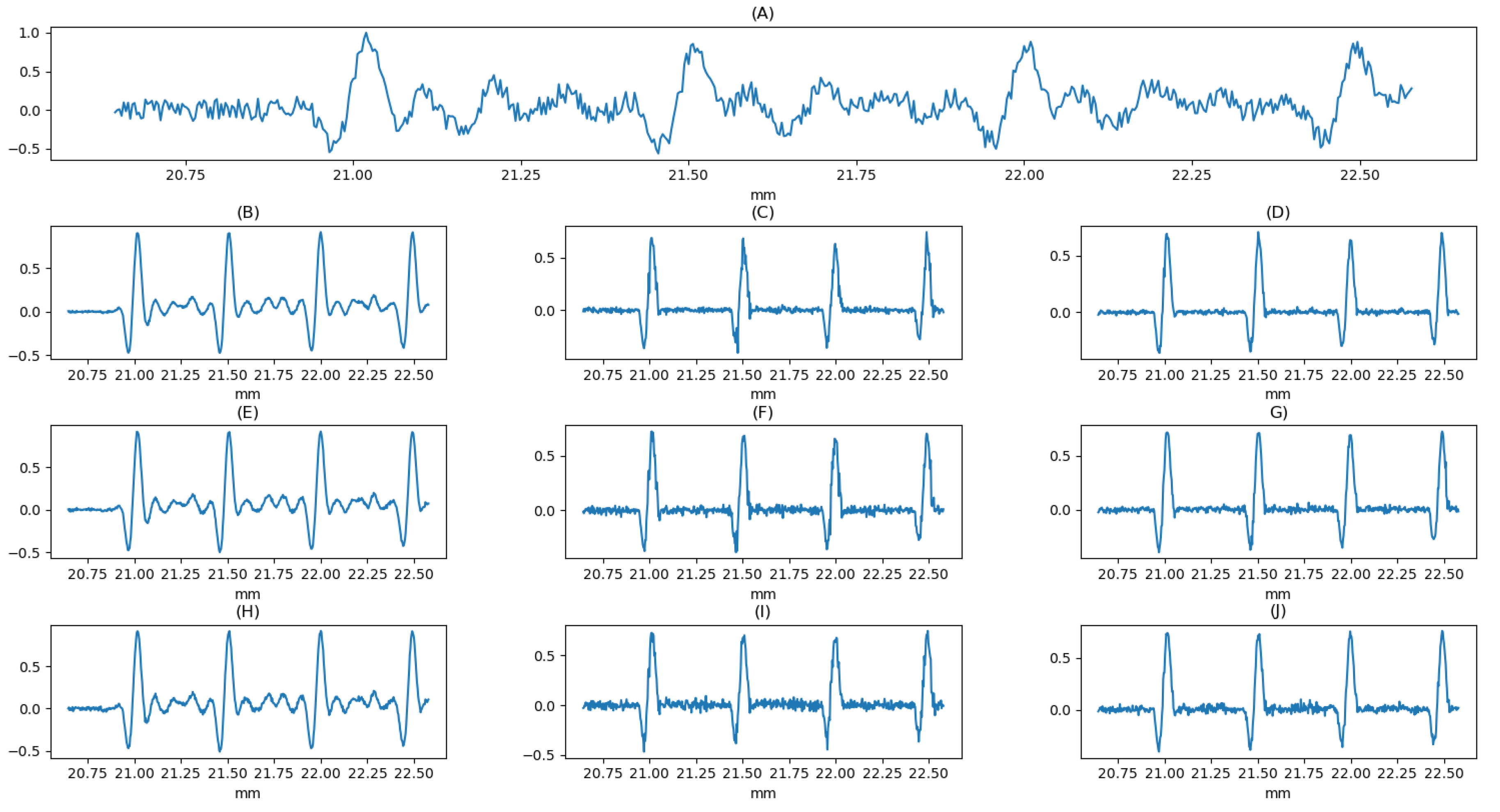
For demonstration purposes, we consider the following example. Using a line of reflectors distributed along the Z-axis every 250 microns as a reference, we simulated 128, 64, and 32 different emission apertures and observed (Figure 10) the acquisition at a specific element located at position . For these signals, knowing that they all correspond to the same scene and share common elements, we applied three different processing methods to reduce noise.
The first method is averaging, which eliminates electronic noise but is not sufficient to remove the secondary oscillation characteristic of a flat wavefront (B, E, H). The second method is minimum selection, an aggressive solution that provides high contrast without secondary lobes, but is highly dependent on the random implementation of apertures and introduces high-frequency noise typical of nonlinear systems (C, F, I). The third method is a hybrid solution: with each transmission, we contribute a new estimate for each sample. For each sample, we select a subset of the estimates with the lowest amplitude and compute their average. The number of estimates used in the subset depends on the desired level of smoothness; in this case, we averaged the four lowest values (D, G, J).
The original signal is presented in Figure A. In the simulation, additive noise was introduced at a level of 20 dB relative to the maximum peak amplitude of all the acquisition. Figure 10 (B, C, D) correspond to 128 emissions; Figure 10 (E, F, G) to 64 emissions; and Figure 10 (H, I, J) to 32 emissions. Disregarding the arithmetic mean—which does not yield a significant improvement—the most favorable results are obtained using either the minimum value or the mean of the minimums. Evidently, as the number of acquisitions increases, the likelihood of achieving a more accurate reconstruction also improves. When the acquisition count is high, the mean of the minimums produces highly satisfactory results. However, under constraints on the number of shots, employing the minimum value in combination with suitable filtering techniques offers a robust and efficient compromise.
It is worth to note that this approach requires more time because of time-of-flight limitations, but because averaging is performed before beamforimng, it can be done in hardware, saving bandwidth between the acquisition system and the processing PC, which is a very limited resourc
4.2. Sparse Emission Aperture. Outer Region
Given that the system operates within the near-field region, and considering that plane wave propagation is constrained by the projection of the radiating surface, the scanning area can be extended by employing a ring-shaped emission configuration. This approach enables sonification of regions beyond the lateral range of .
To implement this, the aperture is structured into concentric rings derived from bin segmentation. The dispersion strategy must be carefully designed to suppress edge effects that could lead to elevated secondary lobe levels, while ensuring coverage over a broad spatial domain to promote diversity in field distributions. Accordingly, the secondary ring is selected within the bin structure, maintaining one element per bin in both the outermost ring and the immediately adjacent inner ring (see Figure 5).
This configuration is analyzed in Figure 11. The ring-based arrangement ensures uniform participation across array elements. However it emits lower energy than the Taylor apodization. The average participation distribution spans a wide area, including the projected footprint of the elements. The Gini coefficient rapidly converges toward an equilibrium state, indicating that element participation becomes balanced from a radial distance of 15 mm onwards. It is observed that, despite the uniform weighting, this configuration involves a portion of the aperture in which the maximum element contribution is 5 dB lower than in the Taylor configuration 7.
Based on this strategy, four aperture configurations were designed, and the resulting fields and corresponding planar wavefronts were computed (Figure 12). All configurations exhibit a planar wavefront formed within the region between 2.5 mm and 5 mm, leaving the central zone () with a decay margin ranging from 6 to 12 dB and a disordered distribution. This behavior helps reduce the presence of imaging artifacts originating from the central region.
As in the inner region case, diversity can be leveraged to mitigate artifacts caused by the trailing components following the planar wavefront. The Figure 14 presents the results of applying mean, minimum, and averaged-minimum processing across 128, 64, and 32 acquisitions, respectively, for a sequence of points distributed along the axis at (x = 3 mm, y = 0 mm).
Figure 13.
The figure shows the signal received by an element located at position , corresponding to a plane wave emission performed using a series of random apertures defined according to a Ring-shaped apodization. The simulation includes attenuation caused by coupling, and 20dB of noise has been added relative to the echo with the highest gain. In Figure (A), the signal obtained from a single shot is shown. Figures (B), (C), and (D) correspond to 128 shots and represent, respectively, the mean, the minimum, and the mean of the four lowest values. Figures (E), (F), and (G) correspond to 64 shots and likewise represent the mean, the minimum, and the mean of the four lowest values. Figures (H), (I), and (J) correspond to 32 shots and again represent the mean, the minimum, and the mean of the four lowest values.
Finally, Figure 14 shows the diffraction pattern of the two emission apertures within the plane of interest. To assess how they complement each other, a combined representation of the mean field from both configurations is also included. It should be noted that the insonification strategy for the outer region is 10 dB lower than that of the inner region. This aspect must be taken into account when combining both results.
4.3. Sparse Reception Aperture
The emission from multiple apertures during reception, combined with the use of nonlinear operators such as the minimum, enables the acquisition of echoes with broad bandwidth and suppresses the influence of secondary wavefronts—one of the main causes of reduced image quality in plane wave imaging. Moreover, this approach helps avoid the presence of grating lobes, thereby simplifying the design of reception apertures.
Under these conditions, an isolated target imaged with a full 32×32 narrowband aperture would theoretically yield a dynamic range of approximately –30 dB. A sparse aperture with 256 elements could reach –18 dB. In scenarios with multiple targets, the interaction of various secondary wavefront patterns reduces these margins.
To establish a reference (see Figure 15), we computed the image generated by the full aperture for a series of targets distributed along the axis (X = 0, Y = 0), and present a detailed view. Additionally, we show the signal received at the element located at (0.3, –0.15) for this image. As observed, the secondary wavefronts from the plane wave introduce oscillations that elevate the background amplitude, thereby reducing the dynamic range.
Figure 14.
The figure shows how the two emission modes complement each other in a plane wave emission with a deflection angle of 0o. Figure (A) displays the field generated by a Taylor apodization. Figure (B) shows the field generated by a ring-shaped aperture. Figure (C) presents the average of both fields. Although they complement each other well, a drop of approximately 10dB is observed between the Taylor apodization (red line) and the ring-shaped apodization (blue line).
By applying our emission taylor-based dispersion strategy and mitigating plane wave interferen, it becomes feasible to reconstruct the full aperture in reception using four acquisitions of 256 elements. In the Figure 15-C, we present the resulting image and the signal received at the same central element than the full aperture. Although our approach incurs some loss of reflectivity in certain targets due to emitting with only one-fourth of the elements, the resulting image exhibits an increased dynamic range and reveals the underlying interference structure between the secondary lobes of each reflector.
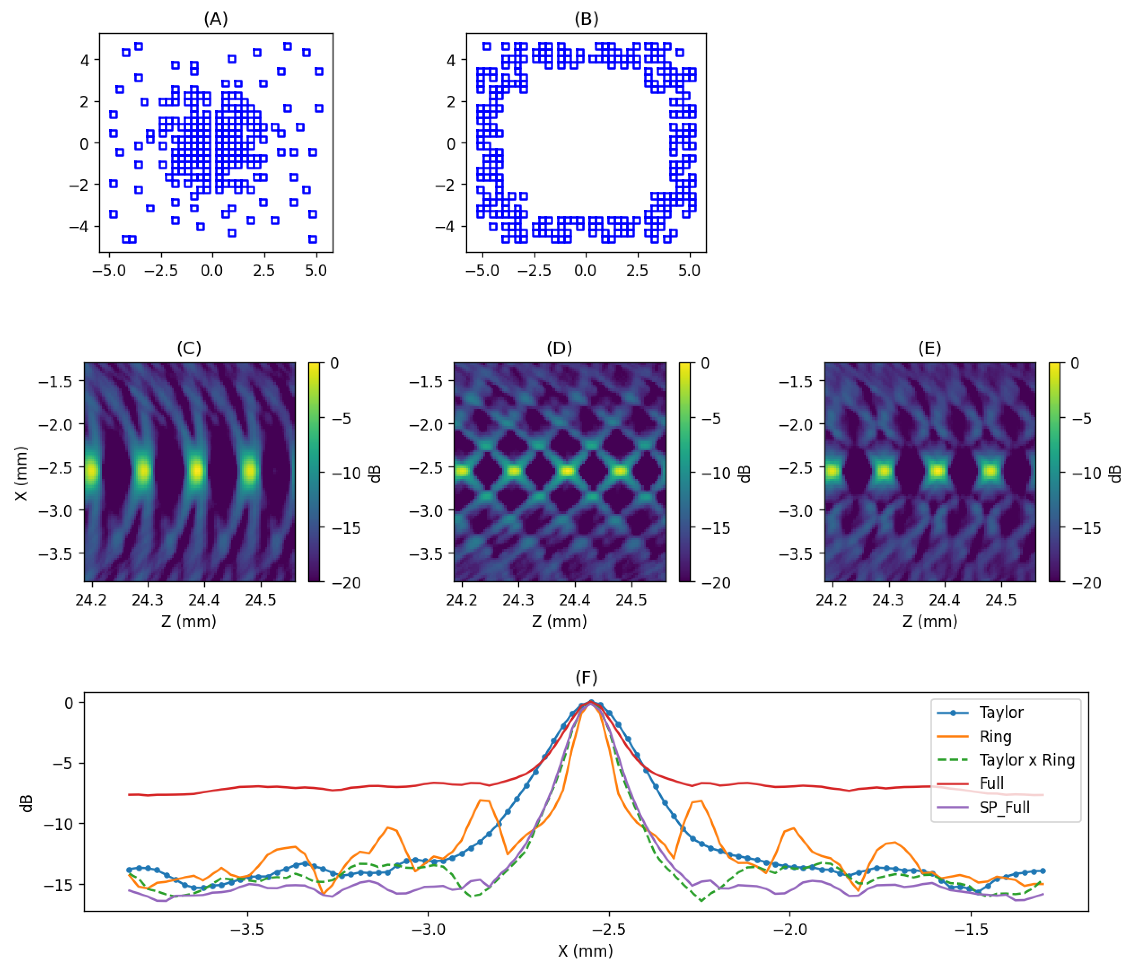
Once the distortion introduced by planar emission has been mitigated, the design of the reception aperture becomes a more classical problem, primarily focused on ensuring contrast and lateral resolution. This is constrained by technical factors such as the number of elements and their sensitivity, as illustrated in Figure 4. This Figure presents various dispersion cases designed following the strategies described in Figure 5. In Figures (A) and (C), we show an aperture following a Taylor apodization—commonly used in reception—and its corresponding image. This configuration emphasizes the suppression of secondary lobes but results in poor lateral resolution. In Figures (B) and (D), we present an aperture arranged in a ring distribution, selected to enhance lateral resolution, along with its corresponding image. This setup improves resolution but exhibits elevated side lobes, which reduce the dynamic range.
Figure (E) shows a hybrid solution obtained by computing the geometric mean of the two previous images, partially combining the advantages of both strategies. For comparison, Figure (F) displays the peak profile along the Z-axis for all four configurations, alongside the full aperture (FULL). In general, all proposed solutions exhibit twice the contrast of the FULL configuration. The solution offering the highest contrast is the one that reconstructs the full aperture using four emissions (SP FULL), while the RING configuration provides the best lateral resolution. The hybrid solution between RING and Taylor offers a balanced compromise, achieving performance close to SP FULL with only two acquisitions instead of four.
Figure 16.
For the same scenario described in Figure 15, the image obtained using a reception aperture based on (A, C) Taylor apodization and (B, D) a ring-shaped aperture mounted on the outer bins is presented. Additionally, the image generated from the geometric mean between (C) and (D) is shown. Figure (F) displays the lateral profile of the five reception configurations considered.
5. Results
To evaluate a more complex scenario, three double-point curves were designed, spaced 125 microns apart in the Z-axis and 500 microns in the X-axis. This configuration is illustrated in Figure 17, which shows the image obtained using the full aperture. In the image, the targets are visible but exhibit a very low dynamic range, close to 3 dB.
For the same scenario, we will compute the image using our emission dispersion scheme with two regions of interest, and under two different reception conditions. First, using the full aperture reconstructed from four complementary acquisitions; and second, using a ring-shaped aperture combined with Taylor apodization, based on the geometric mean of the acquisitions.
In the first case (see Figure 18), the two regions are presented separately. For the inner region, the image displays only the central part of the scene, which is reconstructed with good resolution and a dynamic range close to 15 dB. In contrast, the image of the outer region, while maintaining resolution, shows a reduction of approximately 50% in dynamic range.
Considering the entire process, once the reception aperture is defined and used as the basis for signal acquisition in both regions, the processed signals corresponding to the same reception element can be summed within the same reception channel buffers. This effectively compacts data from both regions into a single signal. This operation can be directly managed by the acquisition system, maintaining a data flow equivalent to that of a single acquisition, while also compressing the entire image. Once the signals are collected, the beamforming process can be applied across the entire region of interest.
In Figure 18(C), both images are combined by merging the data during the beamforming process (which can also be performed in the reception channels). To preserve balance in the final image, the central region was attenuated by 6 dB.
Finally, Figure 19 shows the result of combining the Taylor and ring strategies in reception. In these two cases, the two regions are already presented as combined (Figure 19A–B), and the following image displays the result of applying the geometric mean between both apertures. The outcome is similar to that presented in Figure 18 with two reception apertures instead of four.
6. Discussion
This study analyzes the performance of a two-dimensional array with large elements for near-field imaging, specifically targeting applications in preclinical cerebrovascular research. Under these conditions, the aperture must operate effectively at very short distances, support high-speed acquisition modes, and be adaptable to systems with a limited number of active channels.
Metrics were obtained to evaluate the contribution of individual elements to image formation, and optimal operating conditions were proposed to maximize resource efficiency. Based on the results, and considering certain trade-offs, a viable working range is defined as greater than and up to , with no more than of coupling material.
A novel methodology was developed to exploit transmit aperture diversity and significantly suppress sidelobes generated by plane-wave transmission, using region-specific optimization strategies. Unlike conventional approaches that rely on a single deterministic solution, the proposed method employs multiple transmit apertures randomly selected within the constraints of each strategy, while maintaining a common receive aperture.
Simulations demonstrate that minimizing sample amplitudes effectively reduces noise, suppresses secondary oscillation patterns, and enhances echo bandwidth. This approach eliminates the need for transmit beam steering and enables full operation in plane-wave mode without introducing transmit delays. Additionally, it offers substantial design flexibility for the receive aperture, which is no longer constrained by grating lobe generation.
The analysis indicates that dividing the image area into two regions and adapting the transmission accordingly yields improved performance. However, performance varies between regions due to modulation effects introduced by the elements. The central region achieves the best results, exhibiting a contrast higher than the outer region. Combining both regions during beamforming allows for balancing these differences, but it also transfers secondary lobe patterns between regions and reduces overall dynamic range. A dedicated processing technique is required to merge both regions while minimizing mutual interference.
Technological implementation of this solution involves addressing several key challenges. First, depending on the selected operational mode, the system requires the development of two to three independent multiplexing structures: two for transmission (potentially shared with reception) and one specifically for reception. The first structure uses a Taylor apodization scheme; the second employs a ring-distribution scheme; and the third, dedicated to reception, is designed to cover the full aperture in a maximum of four firings.
Second, since beamforming does not require knowledge of the emission elements’ positions, the system could incorporate a mechanism to autonomously and randomly select transmitting apertures within the constraints of each transmission strategy. Additionally, a processing stage could be implemented in the receiving channels to apply a nonlinear, minimum-based filter functioning as an EMI-like filtering stage [18].
Finally, achieving high-speed imaging depends not only on the time of flight but also on how quickly acquisition buffers are released (i.e., the time required to transfer data to the storage unit). This transfer time is determined by the communication interface. For example, with an acquisition time of 20 microseconds (sampling rate: 65 MHz) and 256 parallel channels, the transfer time can be approximately 220 microseconds using a high-speed 3 GBps interface, or up to 9.2 milliseconds with a standard Gigabit Ethernet interface.
The ability to parallelize data transmission with the acquisition and processing of multiple firings for the next capture would allow up to 5 firings in the first case and 230 in the second. Assuming 10 firings per acquisition and two acquisitions per image (solution based on combined taylor and ring-shape reception profiles), these figures would enable frame rates approaching 1,000 images per second.
In summary, this work provides solutions to the low-contrast issue in plane-wave imaging without requiring wavefront deflection. It optimizes acquisition processes, improves data flow efficiency, and reduces computational cost by enabling full image reconstruction using the same data volume as a single acquisition. Furthermore, the proposed approach simplifies the design of sparse apertures involved in the process, particularly facilitating the design of the reception aperture by minimizing grating lobe generation.
Author Contributions
Conceptualization and methodology, OMG; software, JHM; formal analysis, investigation and validation OMG, LES; resources,MPR, GC and JCS; writing, OMG; review and comments: JCS OMG and LES. All authors have read and agreed to the published version of the manuscript.
Funding
This research work was funded by the European Commission – NextGenerationEU, through Momentum CSIC Programme: Develop Your Digital Talent. This research work was funded by: PID2022 - 138013OB -I00 /MCIN /AEI /10.13039/ 501100011033/ FEDER, UE. This work has been developed within the framework of the LUNABRAIN-CM project, funded with 1,026 million by the Community of Madrid through the R&D activities program in technologies, granted by Order 5696/2024
Institutional Review Board Statement
Not applicable. This study is conducted within a theoretical framework, prior to experimentation, and does not involve the use of animal models.
Acknowledgments
Jorge Huecas, Staff hired under the Generation D initiative, promoted by Red.es, an organisation attached to the Ministry for Digital Transformation and the Civil Service, for the attraction and retention of talent through grants and training contracts, financed by the Recovery, Transformation and Resilience Plan through the European Union’s Next Generation funds. This research work was funded by the European Commission – NextGenerationEU, through Momentum CSIC Programme: Develop Your Digital Talent This research work was funded by: PID2022 - 138013OB -I00 /MCIN /AEI /10.13039/ 501100011033/ FEDER, UE This work has been developed within the framework of the LUNABRAIN-CM project, funded with 1,026 million by the Community of Madrid through the R&D activities program in technologies, granted by Order 5696/2024
Conflicts of Interest
The authors declare no conflicts of interest. The funders had no role in the design of the study; in the collection, analyses, or interpretation of data; in the writing of the manuscript; or in the decision to publish the results.
References
- J. Provost et al., 3D ultrafast Doppler imaging applied to the noninvasive mapping of blood vessels in vivo, IEEE Trans. Med. Imaging, vol. 35, no. 4, pp. 1109–1117, Apr. 2016.
- C. Errico et al., Ultrafast ultrasound localization microscopy for deep super-resolution vascular imaging, Nature, vol. 527, pp. 499–502, Nov. 2015.
- Chavignon A, Heiles B, Hingot V, Orset C, Vivien D, Couture O. 3D Transcranial Ultrasound Localization Microscopy in the Rat Brain With a Multiplexed Matrix Probe. IEEE Trans Biomed Eng. 69(7):2132-2142. [CrossRef]
- Provost, J. , Garofalakis, A., Sourdon, J. et al. Simultaneous positron emission tomography and ultrafast ultrasound for hybrid molecular, anatomical and functional imaging. Nat Biomed Eng 2, 85–94 (2018). [CrossRef]
- Zhang C, Lei S, Ma A, Wang B, Wang S, Liu J, Shang D, Zhang Q, Li Y, Zheng H, Ma T. Evaluation of tumor microvasculature with 3D ultrasound localization microscopy based on 2D matrix array. Eur Radiol. 2024, 34(8):5250-5259. [CrossRef]
- Li X, Gachagan A, Murray P. Design of 2D Sparse Array Transducers for Anomaly Detection in Medical Phantoms. Sensors. 2020, 20(18):5370. [CrossRef]
- Martínez-Graullera Ó, de Souza JCE, Parrilla Romero M, Higuti RT. Design of 2D Planar Sparse Binned Arrays Based on the Coarray Analysis. Sensors. 2021, 21(23):8018. [CrossRef]
- Maffett R, Boni E, Chee AJY, Yiu BYS, Savoia AS, Ramalli A, Tortoli P, Yu ACH. Unfocused Field Analysis of a Density-Tapered Spiral Array for High-Volume-Rate 3-D Ultrasound Imaging. IEEE Trans Ultrason Ferroelectr Freq Control. 2022, 69(10):2810-2822. [CrossRef]
- Jean-Baptiste Jacquet, Jean-Luc Guey, Pierre Kauffmann, Mohamed Tamraoui, Emmanuel Roux, et al.. Simulation, Design and characterization of a Large Divergent Element Sparse Array (LDESA) for 3D Ultrasound Imaging. IEEE Transactions on Ultrasonics, Ferroelectrics and Frequency Control, In press. [CrossRef]
- Montaldo, G., Tanter, M., Bercoff, J., Benech, P., and Fink, M. Coherent plane-wave compounding for very high frame rate ultrasonography and transient elastography. In IEEE Transactions on Ultrasonics, Ferroelectrics, and Frequency Control, 56(3), 489–506, 2009.
- Heiles B, Correia M, Hingot V, Pernot M, Provost J, Tanter M, Couture O. Ultrafast 3D Ultrasound Localization Microscopy Using a 32 × 32 Matrix Array. IEEE Trans Med Imaging, 2019, 38(9):2005-2015. [CrossRef]
- M. Tanter and M. Fink, Ultrafast imaging in biomedical ultrasound, IEEE Trans. Ultrason. Ferroelectr. Freq. Control, 2014, vol. 61, no. 1, pp. 102–119.
- Gabriel Montaldo, Alan Urban and Emilie Macé, Functional Ultrasound Neuroimaging Annu. Rev. Neurosci. 2022. 45:491–513. [CrossRef]
- Mari Carmen Gómez-de Frutos, et al. Identification of brain structures and blood vessels by conventional ultrasound in rats, Journal of Neuroscience Methods, Volume 346, 2020, 108935, ISSN 0165-0270. [CrossRef]
- Piwakowski, B.; Sbai, K. A new approach to calculate the field radiated from arbitrarily structured transducer arrays. IEEE Trans. Ultrason. Ferroelectr. Freq. Control 1999, 46, 422–440. [Google Scholar] [CrossRef] [PubMed]
- Lerman, R.I., y Yitzhaki, S. (1984), A note on the calculation and interpretation of the Gini coefficient, Economics Letters, 15, 363-368.
- Eva Ferreira and Araceli Garín, Una nota sobre el cálculo del índice de Gini, Estadística Española, vol 39(142), pp. 207–218, 199, Instituto Nacional de Estadística.
- C. Fritsch et al., A pipelined architecture for high speed automated NDE, 1995 IEEE Ultrasonics Symposium. Proceedings. An International Symposium, Seattle, WA, USA, 1995, pp. 833-836 vol. [CrossRef]
- Harput et al., 3-D Super-Resolution Ultrasound Imaging With a 2-D Sparse Array, in IEEE Transactions on Ultrasonics, Ferroelectrics, and Frequency Control, vol. 67, no. 2, pp. 269-277, Feb. 2020. [CrossRef]
Figure 1.
Prototype of an experimental high-frequency single-transducer ultrasound system, developed within the framework of project PID2022-138013OB-I00 (MCIN/AEI/10.13039/501100011033/FEDER, EU), which served as a precursor to the proposal presented in this work.
Figure 1.
Prototype of an experimental high-frequency single-transducer ultrasound system, developed within the framework of project PID2022-138013OB-I00 (MCIN/AEI/10.13039/501100011033/FEDER, EU), which served as a precursor to the proposal presented in this work.
Figure 2.
(A) The element configuration of the array. (B) Steering capabilities of the full aperture, from ::, and evolution of the beam from :. (C) Evolution of the attenuation with the propagation in the coupling layer and in the biological tissue.
Figure 2.
(A) The element configuration of the array. (B) Steering capabilities of the full aperture, from ::, and evolution of the beam from :. (C) Evolution of the attenuation with the propagation in the coupling layer and in the biological tissue.
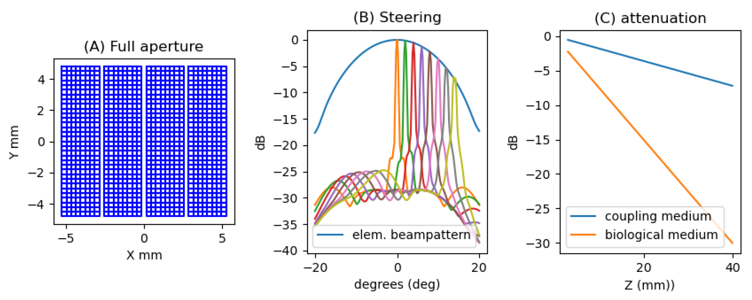
Figure 3.
Bempattern for planar emission in nearfield cases of (A) , (B) , and (D) . (C) lateral profile at with steering from ::.
Figure 3.
Bempattern for planar emission in nearfield cases of (A) , (B) , and (D) . (C) lateral profile at with steering from ::.
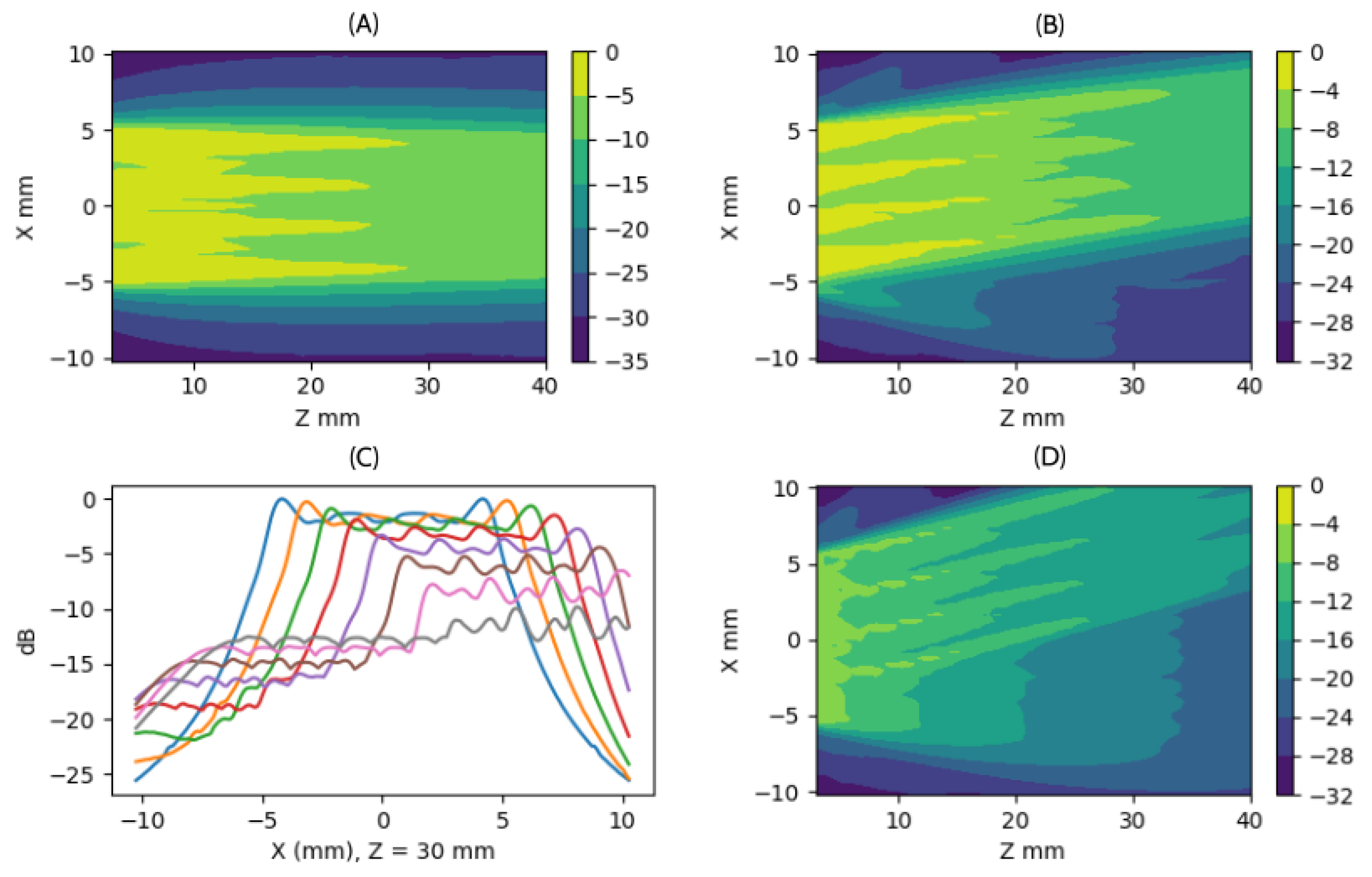
Figure 4.
For full aperture analysis at different points in space, we considered the region and . Figures A–C show the amplitude with which the aperture elements influence three points along the axis at depths of (A) , (B) , and (C) . Taking the mean value as a reference, we observe differences ranging from up to 40 dB in (A) to around 6 dB in (C). Figure D shows the average gain level exerted at each point in the plane. The values in (E) represent the level reached by elements below the mean, while (F) shows the values above it. In (G), we present the statistical dispersion of these values, calculated using the Gini coefficient. Figure (H) displays the percentage of elements below the mean, and Figure (I) shows the percentage above the mean.
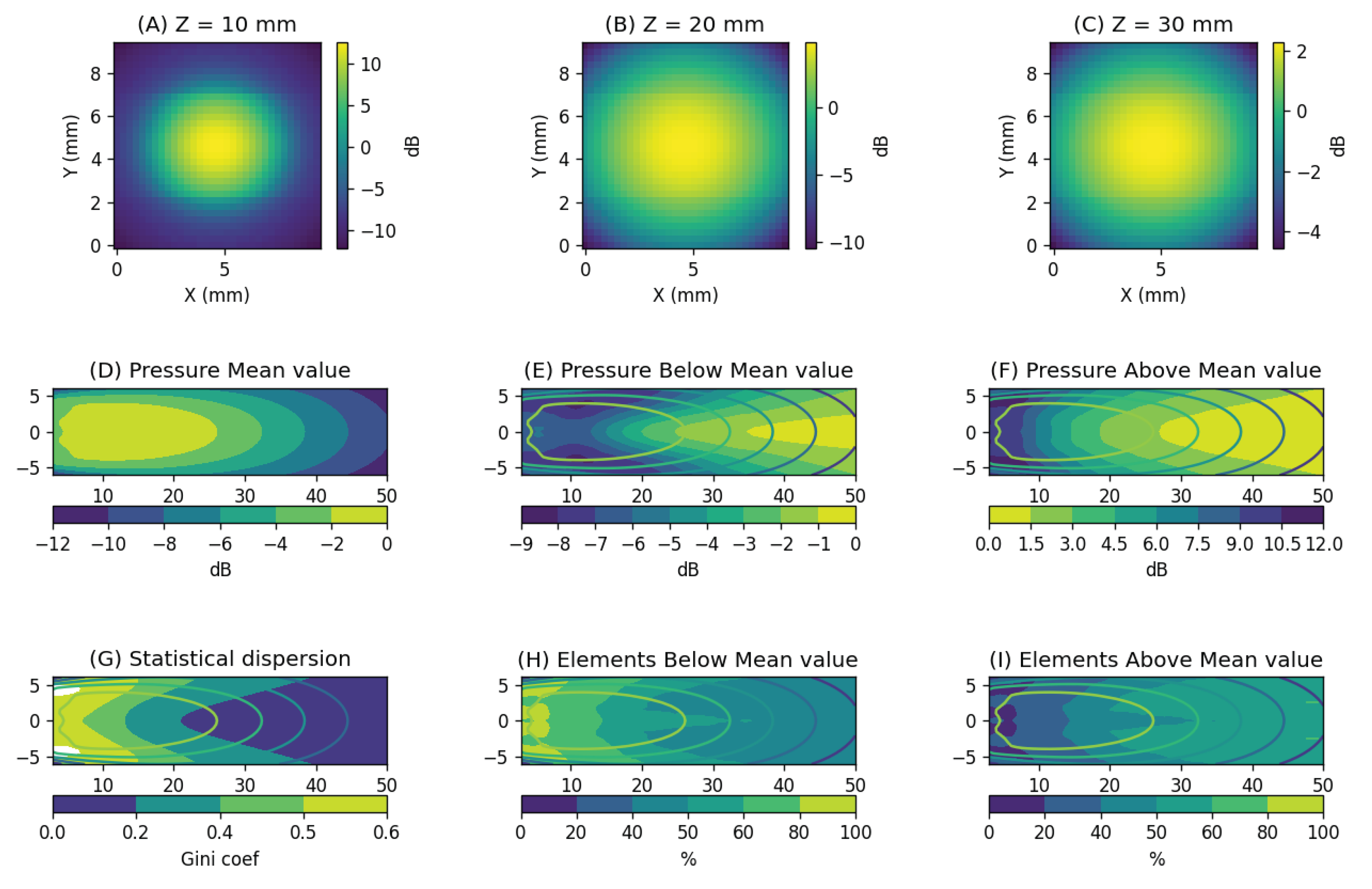
Figure 5.
Three sparsification strategies: (A) transmission and reception, (B) transmission only, (C) reception only.
Figure 5.
Three sparsification strategies: (A) transmission and reception, (B) transmission only, (C) reception only.
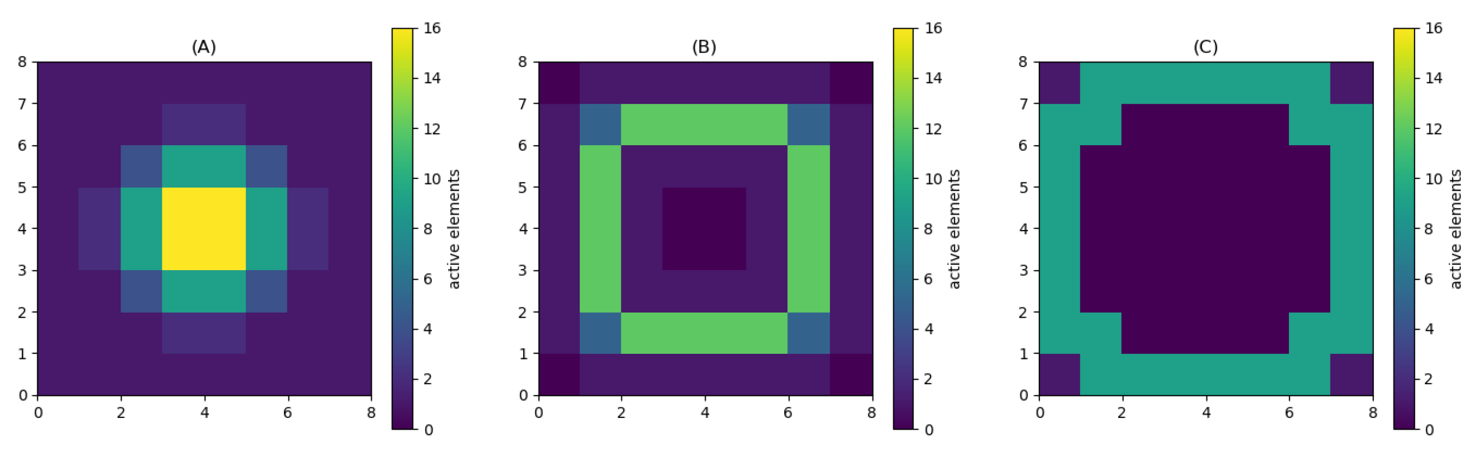
Figure 8.
For a particular realization of the Taylor-apodized aperture shown in Figure (D), Figure (A) displays the field generated by a plane wave emission along the axis . Figure (B) shows the field generated by a deflected plane wave emission at . Figure (C) presents the lateral cross-section of the field at , across angles from to in steps of .
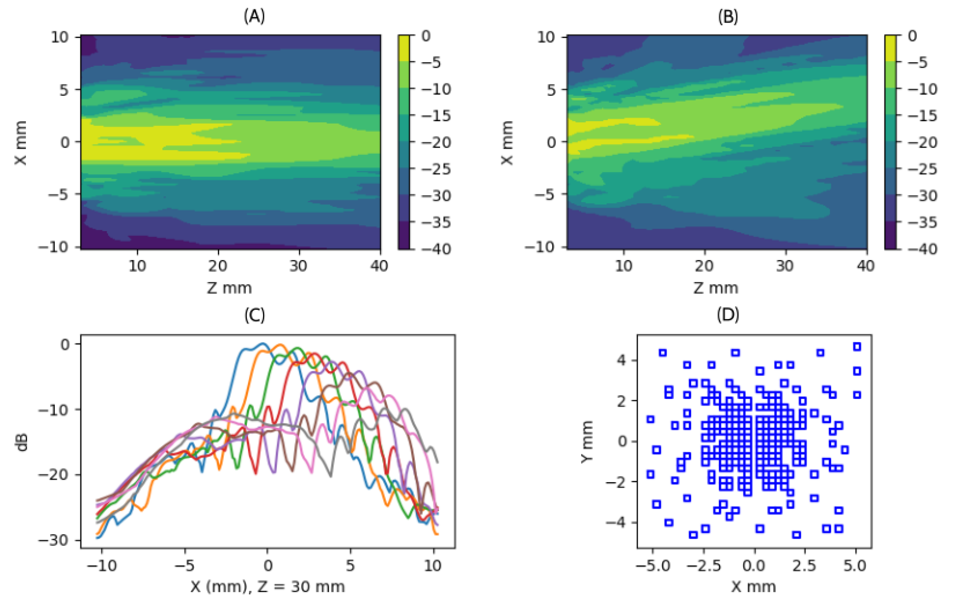
Figure 9.
This figure presents four cases of Taylor apodization realizations. In each column, we show the aperture, the generated field at Z=30mm within the aperture’s projection zone, and the envelope of the wavefront produced by a plane wave emission. The most relevant aspect is the variation observed in the tails of these wavefronts, which are intended to enhance the received signal.
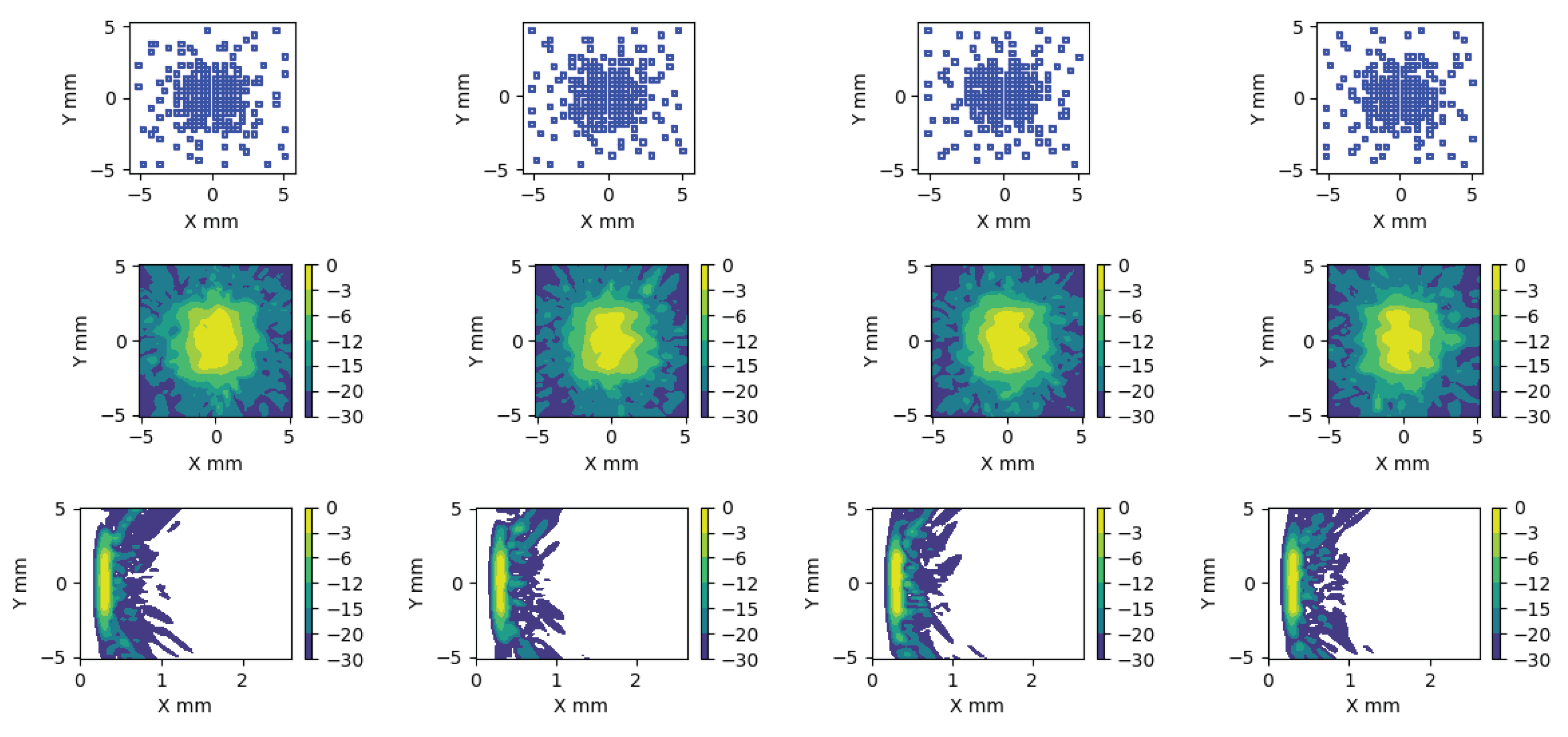
Figure 10.
The figure shows the signal received by an element located at position , corresponding to a plane wave emission performed using a series of random apertures defined according to a Taylor apodization. The simulation includes attenuation caused by coupling, and 20dB of noise has been added relative to the echo with the highest gain. In Figure (A), the signal obtained from a single shot is shown. Figures (B), (C), and (D) correspond to 128 shots and represent, respectively, the mean, the minimum, and the mean of the four lowest values. Figures (E), (F), and (G) correspond to 64 shots and likewise represent the mean, the minimum, and the mean of the four lowest values. Figures (H), (I), and (J) correspond to 32 shots and again represent the mean, the minimum, and the mean of the four lowest values.
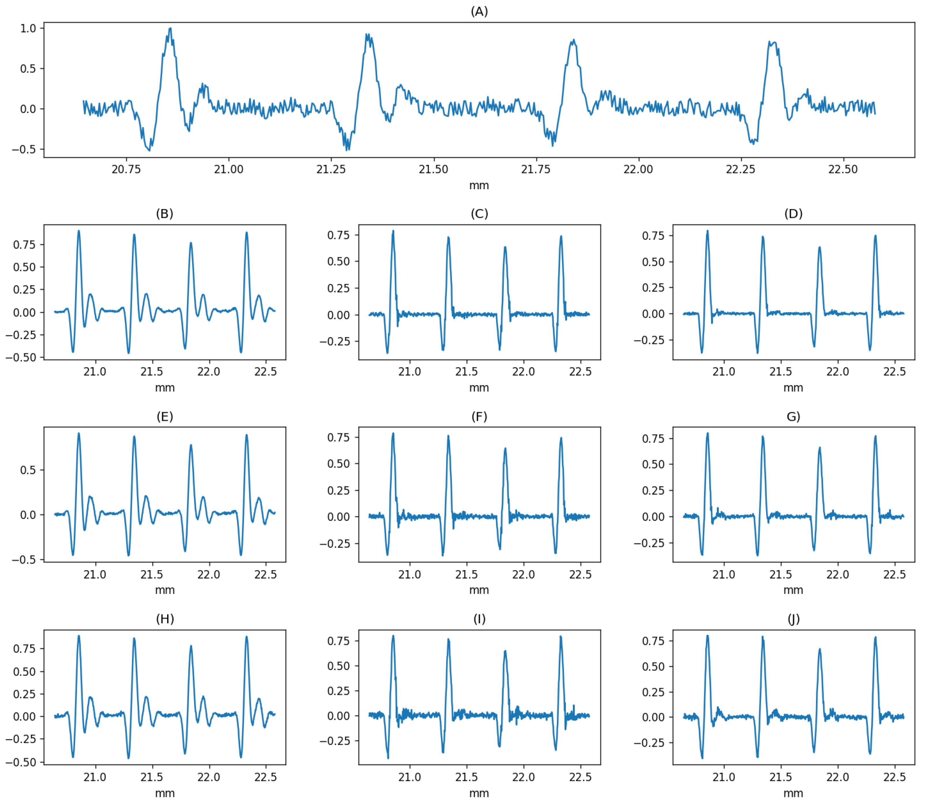
Figure 11.
For the Ring shaped apodized aperture analysis at different points in space, we considered the region and . Figures A–C show the amplitude with which the aperture elements influence three points along the axis at depths of (A) , (B) , and (C) . Taking the mean value as a reference, we observe differences ranging from up to 15 dB in (A) to around 4 dB in (C). Figure D shows the average gain level exerted at each point in the plane. The values in (E) represent the level reached by elements below the mean, while (F) shows the values above it. In (G), we present the statistical dispersion of these values, calculated using the Gini coefficient. Figure (H) displays the percentage of elements below the mean, and Figure (I) shows the percentage above the mean.
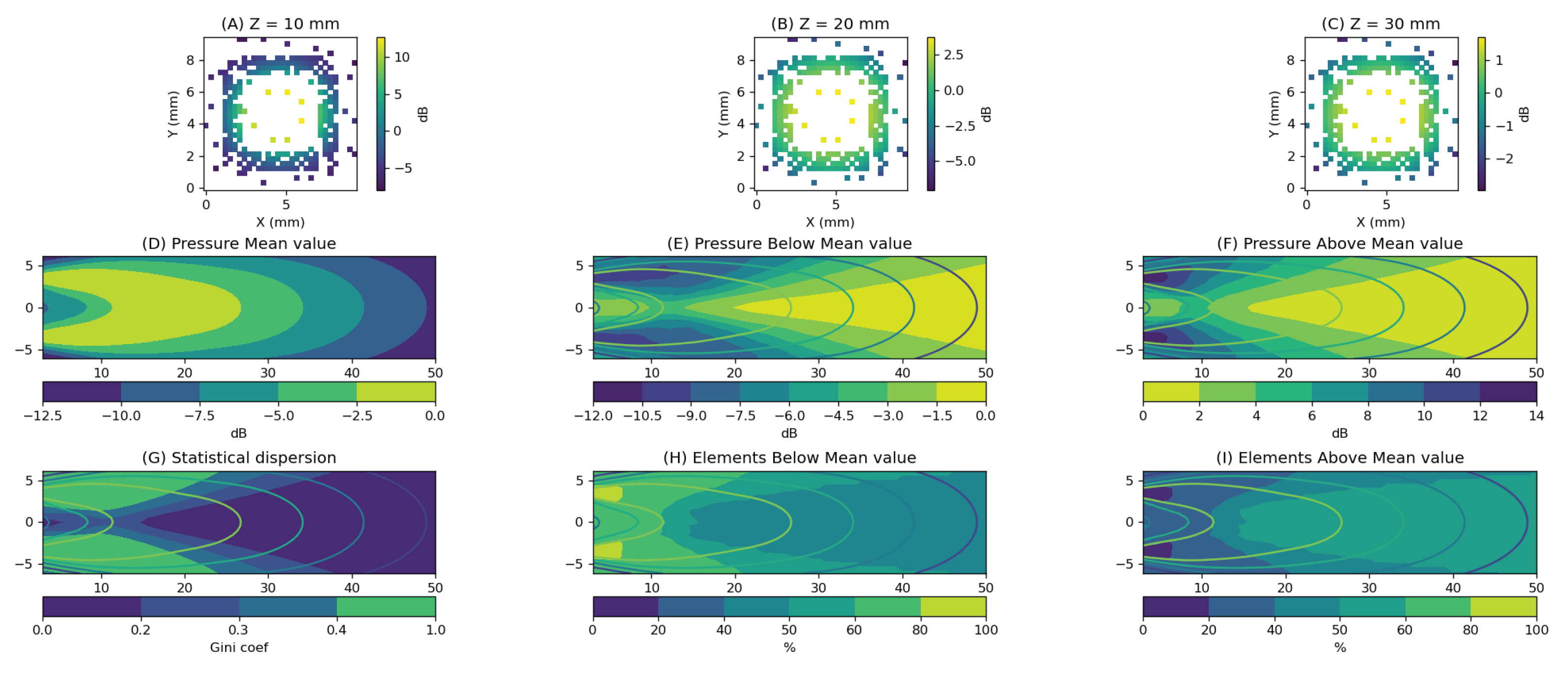
Figure 12.
This figure presents four cases of Ring-shaped apodization realizations. In each column, we show the aperture, the generated field at Z=30mm within the aperture’s projection zone, and the envelope of the wavefront produced by a plane wave emission. The most relevant aspect is the variation observed in the tails of these wavefronts, which are intended to enhance the received signal.
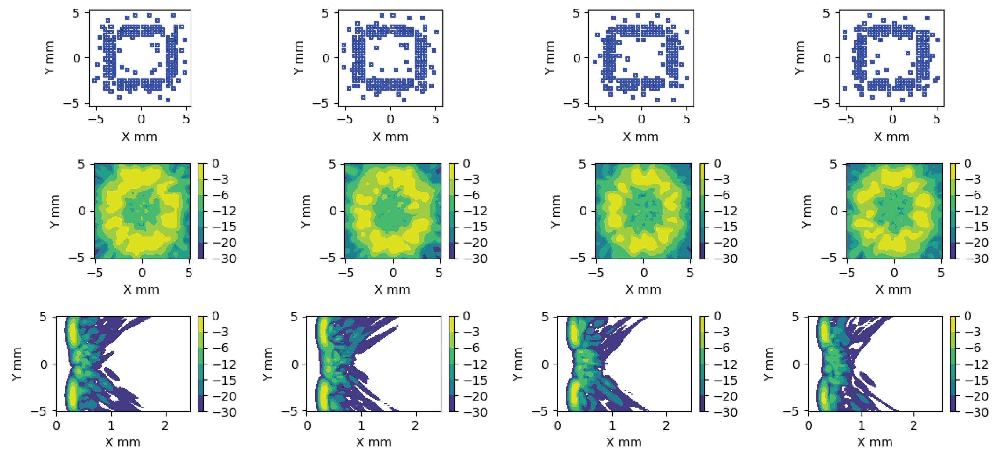
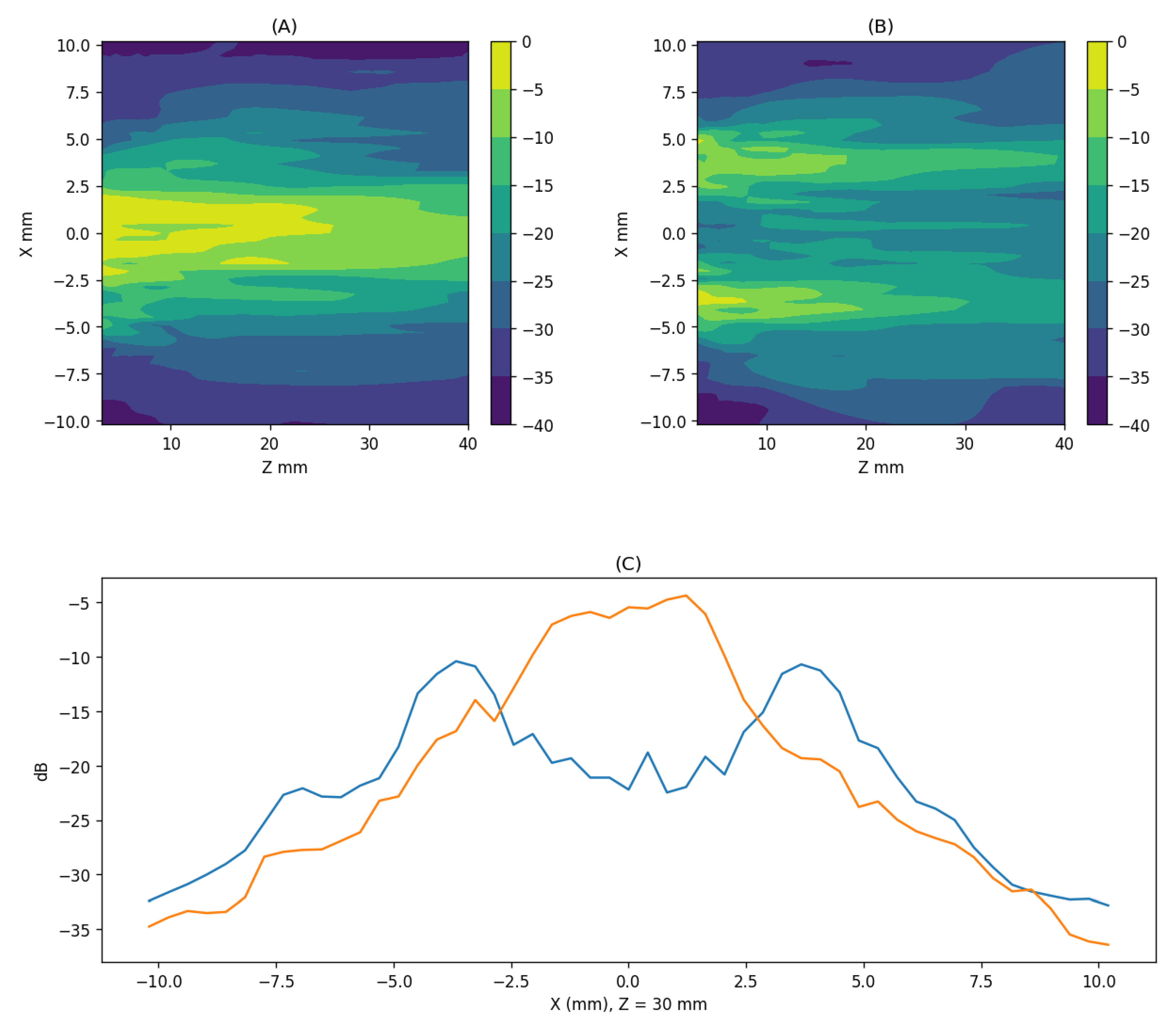
Figure 15.
For a scenario in which a sequence of reflectors spaced 250 microns apart has been placed, image (B) was computed using a full aperture from a flat emission. A composite image was also generated from four acquisitions (A-1,2,3,4), each consisting of eight emissions based on Taylor apodization and processed using minimum absolute techniques (B). Figure (C) shows a detailed view of the signal obtained at the element located at (0.3, -0.15). The signal corresponding to the full aperture emission is shown in blue, while the one corresponding to the Taylor-apodized and minimum-processed emission is shown in orange.
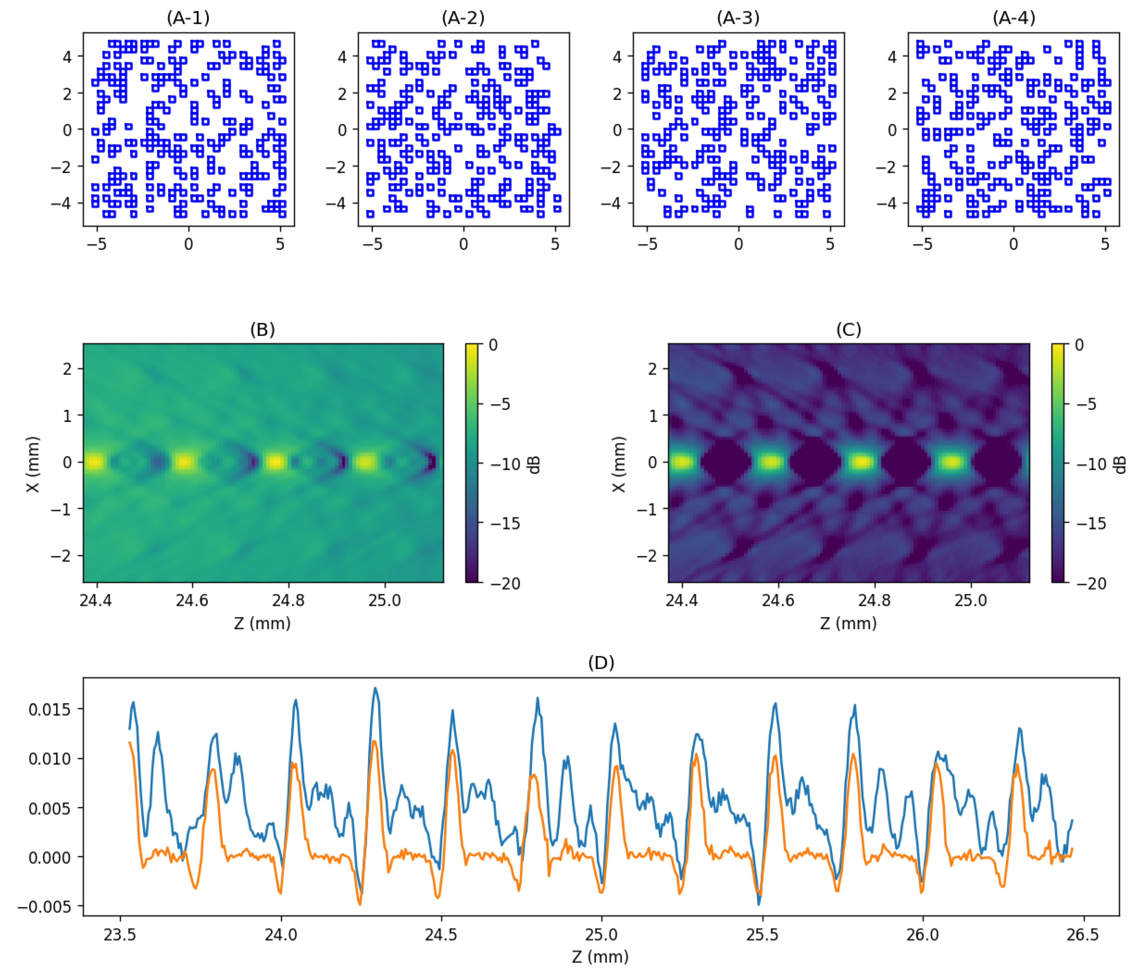
Figure 17.
Image generated using plane wave emission with a deflection angle of and full aperture. The scenario consists of three curves formed by pairs of points spaced 125 microns apart in the X direction and 500 microns in the Z direction.
Figure 17.
Image generated using plane wave emission with a deflection angle of and full aperture. The scenario consists of three curves formed by pairs of points spaced 125 microns apart in the X direction and 500 microns in the Z direction.
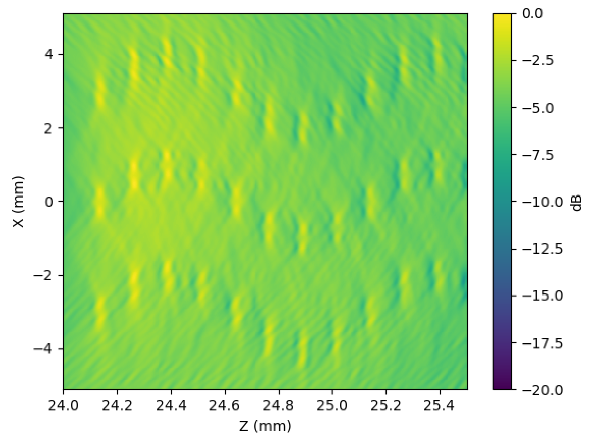
Figure 18.
Image generated using plane wave emission with a deflection of . The scenario consists of three curves formed by pairs of points spaced 125 microns apart in the X direction and 500 microns in the Z direction. The image was obtained from four acquisitions using 256 receiving elements, completing the full aperture. In (A), the image corresponds to emissions using Taylor apodization (8 shots processed with minimum variance). In (B), the image corresponds to emissions using ring-shaped apodization (8 shots processed with minimum absolute). In (C), the final image is obtained by summing the signals from both emissions, already processed with minimum variance, over the same reception channels prior to beamforming.
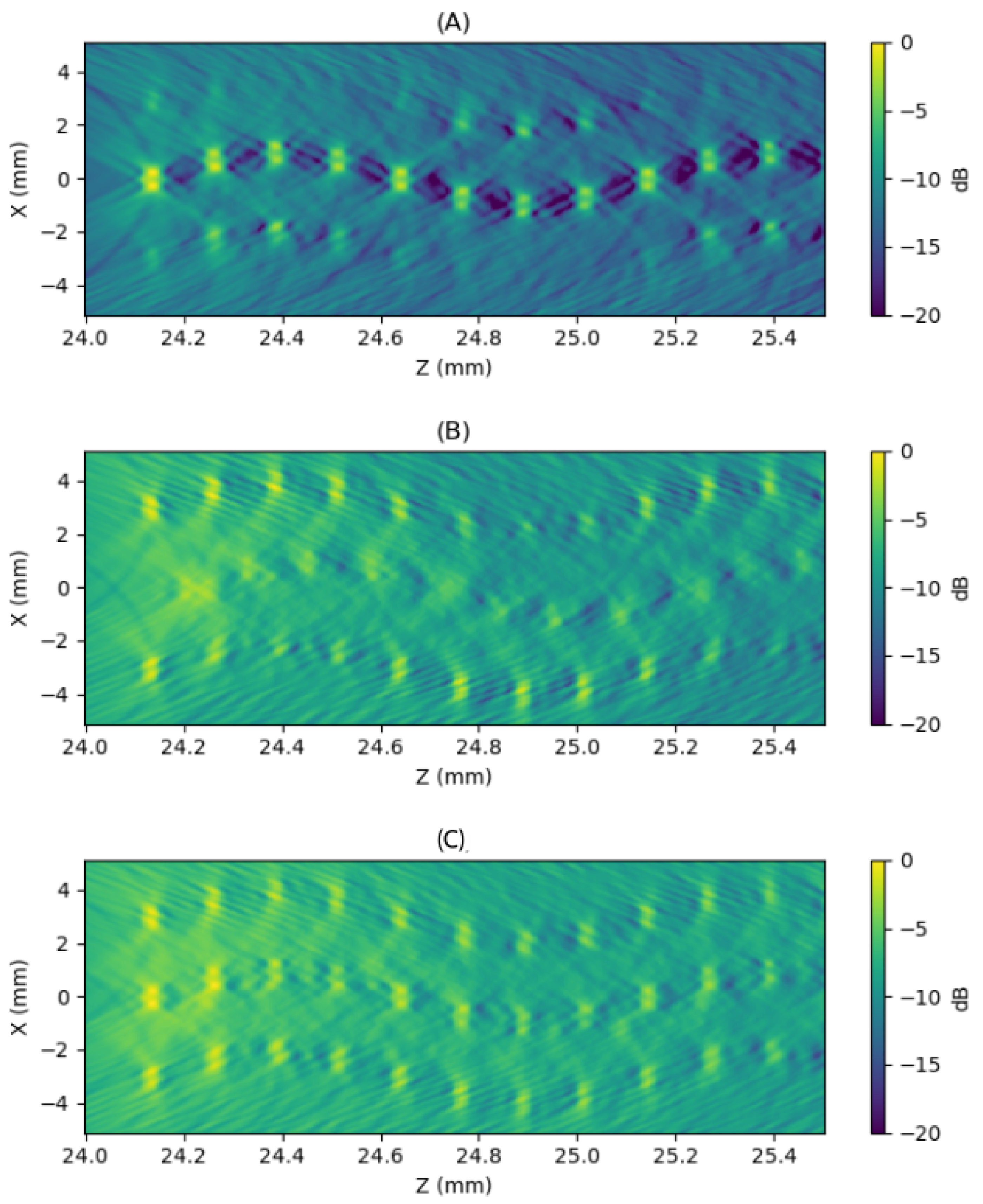
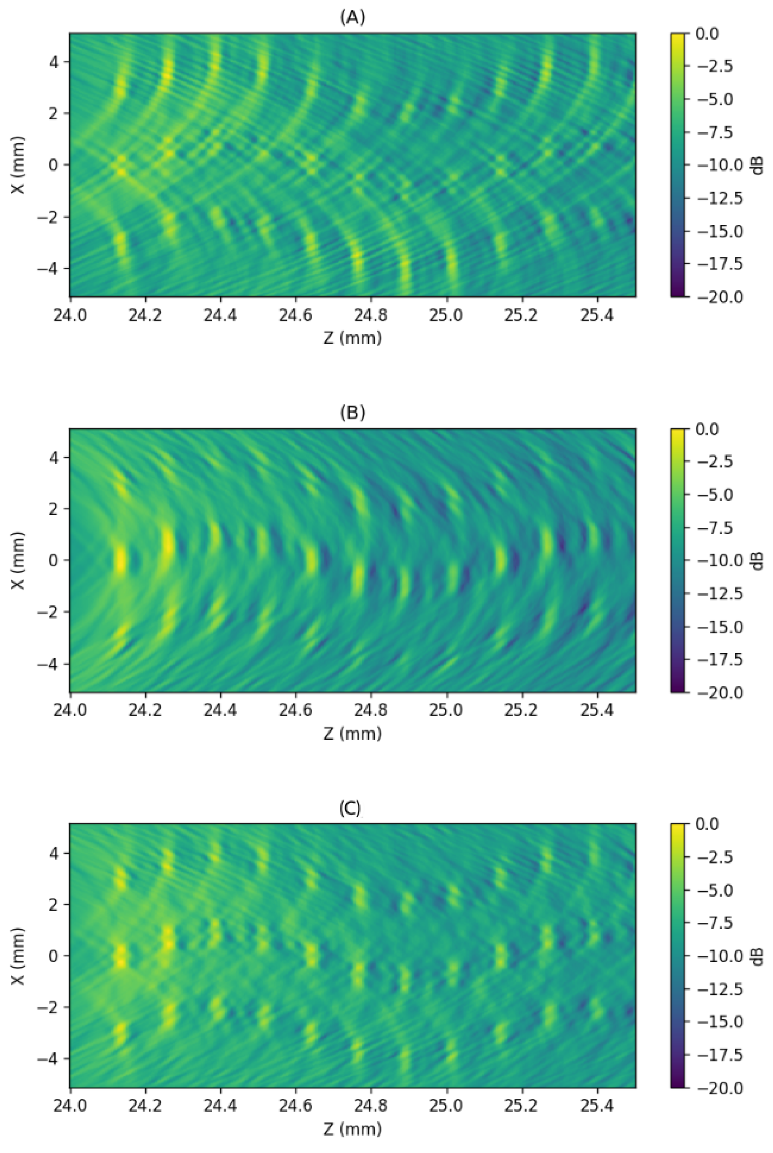
Figure 19.
Image generated using plane wave emission with a deflection angle of . The scenario consists of three curves formed by pairs of points spaced 125 microns apart in the X direction and 500 microns in the Z direction. Image (A) was obtained using 256 receiving elements, modeled with a Taylor apodized aperture, by summing the signals from both emissions (already processed with minimum absolute) over the same reception channels prior to beamforming. Image (B) was obtained using 256 receiving elements, modeled with a ring-shaped aperture, also by summing the signals from both emissions (processed with minimum absolute) over the same reception channels prior to beamforming. Figure (C) was obtained by combining (A) and (B) using a geometric mean.
Disclaimer/Publisher’s Note: The statements, opinions and data contained in all publications are solely those of the individual author(s) and contributor(s) and not of MDPI and/or the editor(s). MDPI and/or the editor(s) disclaim responsibility for any injury to people or property resulting from any ideas, methods, instructions or products referred to in the content. |
© 2025 by the authors. Licensee MDPI, Basel, Switzerland. This article is an open access article distributed under the terms and conditions of the Creative Commons Attribution (CC BY) license (http://creativecommons.org/licenses/by/4.0/).
Copyright: This open access article is published under a Creative Commons CC BY 4.0 license, which permit the free download, distribution, and reuse, provided that the author and preprint are cited in any reuse.


