MetaStructures and Iterated MetaStructures: Extensions to Ontology, Computing, Puzzle, Logic, Ethics, Data and Governance

1. Preliminaries

We first collect the basic notions and notation used throughout the paper. Unless explicitly stated otherwise, all sets and structures considered here are finite.

1.1. Classical Structure

In this work, a Structure is understood broadly as a mathematical system that may arise in Set Theory, Logic, Probability and Statistics, Algebra, Geometry, and related domains.

Definition 1

(Classical Structure). (cf. [1,2]) A  Classical Structure  $\mathcal{C}$ is a mathematical object originating from a traditional area (e.g., Set Theory, Logic, Probability, Statistics, Algebra, Geometry, Graph Theory, Automata Theory, or Game Theory). Formally, write

$$\mathcal{C}=\left(H,{\left\{{\#}^{\left(m\right)}\right\}}_{m\in \mathcal{I}}\right),$$

where:

• H is a nonempty carrier (universe);
• for each $m\in \mathcal{I}\subseteq {\mathbb{Z}}_{>0}$, there is an m-ary operation

  $${\#}^{\left(m\right)}:H^m⟶H,$$
  subject to axioms appropriate to the intended structure (e.g., associativity, commutativity, identities, inverses).

The family ${\left\{{\#}^{\left(m\right)}\right\}}_{m\in \mathcal{I}}$ specifies the type of $\mathcal{C}$. Illustrative instances include:

• Set$(S,⌀)$: a pure carrier possibly with designated elements/relations but no operations [3,4].
• Logic$(L,\wedge ,\vee ,\neg )$: binary connectives $\wedge ,\vee$ and a unary connective ¬, validating the usual logical laws [5].
• Probability space$(\Omega ,\mathcal{F},P)$: a probability measure $P:\mathcal{F}\to [0,1]$ on a σ-algebra $\mathcal{F}\subseteq \mathcal{P}(\Omega )$ [6,7].
• Statistical model$(X,\mathcal{A},\theta )$: data space X, σ-algebra $\mathcal{A}$, and parameter mapping/selector θ [8,9].
• Algebraic structures :

  –

  Group$(G,*)$: $*:G\times G\to G$ with associativity, identity, and inverses [10,11].

  –

  Ring$(R,+,\times )$: two binary operations satisfying the ring axioms [12,13].

  –

  Vector space$(V,+,·)$ over a field $\mathbb{F}$: scalar action $·:\mathbb{F}\times V\to V$ with the usual axioms [14,15,16].

• Metric structure$(X,\mathrm{dist})$ with $\mathrm{dist}:X\times X\to \mathbb{R}$ a metric.
• Graph$(V,E)$: for undirected graphs $E\subseteq \left\{\right\{u,v\}\mid u,v\in V\}$; for directed graphs $E\subseteq V\times V$ [17,18,19,20].
• Automaton$(Q,\Sigma ,\delta ,q_0,F)$: states Q, input alphabet Σ , transition function $\delta :Q\times \Sigma \to Q$, start state $q_0\in Q$, and accepting set $F\subseteq Q$ [21,22].
• Game$(N,{\left\{A_i\right\}}_{i\in N},{\left\{u_i\right\}}_{i\in N})$: players N, action sets $A_i$, and payoff functions $u_i:{\prod }_{j\in N}{A}_j\to \mathbb{R}$ [23,24].

Two closely related generalizations, the HyperStructure [25,26,27,28] and the SuperHyperStructure [29,30,31,32], have also been the focus of recent investigations.

1.2. MetaStructure (Structure of a Structure)

Fix a single–sorted, finitary signature

$$\Sigma =\left(\mathsf{Func},\mathsf{Rel},{ar}_{\mathsf{Func}},{ar}_{\mathsf{Rel}}\right),$$

where $\mathsf{Func}$ and $\mathsf{Rel}$ are the sets of function and relation symbols, and ar records arities. A (single–sorted) $\Sigma$-structure is a tuple

$$\mathbf{C}=\left(H,{\left(f^{\mathbf{C}}\right)}_{f\in \mathsf{Func}},{\left(R^{\mathbf{C}}\right)}_{R\in \mathsf{Rel}}\right),$$

with nonempty carrier H , interpretations $f^{\mathbf{C}}:H^m\to H$ for each f of arity m , and relations $R^{\mathbf{C}}\subseteq H^r$ for each R of arity r . Let ${\mathrm{Str}}_{\Sigma }$ denote the class of all such structures.

Definition 2

(MetaStructure over a fixed signature). (cf. [33]) A MetaStructure (i.e., a “structure of structures”) is a pair

$$\mathbb{M}=\left(U,{\left({\Phi }_{\mathsf{\ell }}\right)}_{\mathsf{\ell }\in \Lambda }\right),$$

where:

• $U\subseteq {\mathrm{Str}}_{\Sigma }$ is a nonempty collection of Σ -structures (level–0 objects);
• for each label $\mathsf{\ell }\in \Lambda$ with meta–arity $k_{\mathsf{\ell }}\in \mathbb{N}$, the meta–operation

  $${\Phi }_{\mathsf{\ell }}:U^{k_{\mathsf{\ell }}}⟶U$$
  is specified uniformly by constructors acting on carriers and symbol interpretations:

  $$\begin{array}{cccc}\hfill & {\Gamma }_{\mathsf{\ell }}({\mathbf{C}}_1,\dots ,{\mathbf{C}}_{k_{\mathsf{\ell }}})=H_{\mathsf{\ell }}\hfill & \hfill & (\mathit{carrier}\mathit{built}\mathit{by}A\mathit{functorial}\mathit{recipe});\hfill \\ \hfill & \forall f\in \mathsf{Func}:f^{{\Phi }_{\mathsf{\ell }}({\mathbf{C}}_1,\dots ,{\mathbf{C}}_{k_{\mathsf{\ell }}})}={\Lambda }_{\mathsf{\ell }}^f\left(f^{{\mathbf{C}}_1},\dots ,f^{{\mathbf{C}}_{k_{\mathsf{\ell }}}}\right);\hfill \\ \hfill & \forall R\in \mathsf{Rel}:R^{{\Phi }_{\mathsf{\ell }}({\mathbf{C}}_1,\dots ,{\mathbf{C}}_{k_{\mathsf{\ell }}})}={\Xi }_{\mathsf{\ell }}^R\left(R^{{\mathbf{C}}_1},\dots ,R^{{\mathbf{C}}_{k_{\mathsf{\ell }}}}\right),\hfill \end{array}$$
  where ${\Lambda }_{\mathsf{\ell }}^f$ and ${\Xi }_{\mathsf{\ell }}^R$ depend only on $f,R,\mathsf{\ell }$ and produce the corresponding output interpretations over $H_{\mathsf{\ell }}$.

Each ${\Phi }_{\mathsf{\ell }}$ is isomorphism–invariant (natural): given isomorphisms ${\alpha }_i:{\mathbf{C}}_i\stackrel{\cong }{\to }{\mathbf{D}}_i$ for $1\le i\le k_{\mathsf{\ell }}$, there is an induced isomorphism

$${\Phi }_{\mathsf{\ell }}({\alpha }_1,\dots ,{\alpha }_{k_{\mathsf{\ell }}}):{\Phi }_{\mathsf{\ell }}({\mathbf{C}}_1,\dots ,{\mathbf{C}}_{k_{\mathsf{\ell }}})\stackrel{\cong }{\to }{\Phi }_{\mathsf{\ell }}({\mathbf{D}}_1,\dots ,{\mathbf{D}}_{k_{\mathsf{\ell }}}),$$

compatible with all function and relation symbols of Σ.

1.3. Iterated MetaStructure (Structure of Structure of ⋯ of Structure)

An Iterated MetaStructure arises by repeatedly applying the MetaStructure construction, producing successive levels where “structures of structures” form a hierarchical tower (cf. [33,34,35,36]).

Definition 3

(Iterated MetaStructure of depth t ). (cf. [33]) For $t\in \mathbb{N}$, an Iterated MetaStructure of depth tover Σ is a MetaStructure ${\mathfrak{M}}^{\left(t\right)}$ obtained by t successive applications of a lifting procedure. If $s<t$, lift a height–s MetaStructure ${\mathfrak{M}}^{\left(s\right)}=(U^{\left(s\right)},\left\{{\odot }_i\right\},\left\{{\mathcal{S}}_j\right\})$ to height t via

$${\iota }_{s\to t}:U^{\left(s\right)}\stackrel{{\mathsf{U}}_{\Sigma }^{t-s}}{\to }{U}^{\left(t\right)}:={\mathsf{U}}_{\Sigma }^{t-s}\left(U^{\left(s\right)}\right),$$

and, for each meta–operation ${\odot }_i:{\left({\mathsf{E}}_{\Sigma }^{m_i}\right)}^{k_i}\to {\mathcal{P}}^{n_i}\left({\mathsf{E}}_{\Sigma }^{n_i}\right)$, define its lift by

$${\odot }_i^{\uparrow }:{\left({\mathsf{E}}_{\Sigma }^{m_i+t-s}\right)}^{k_i}⟶{\mathcal{P}}^{n_i}\left({\mathsf{E}}_{\Sigma }^{n_i+t-s}\right),{\odot }_i^{\uparrow }\left({\mathsf{U}}_{\Sigma }^{t-s}\left(x_1\right),\dots ,{\mathsf{U}}_{\Sigma }^{t-s}\left(x_{k_i}\right)\right):={\mathsf{U}}_{\Sigma }^{t-s}\left({\odot }_i(x_1,\dots ,x_{k_i})\right),$$

and similarly for relations, ${\mathcal{S}}_j^{\uparrow }:={\left({\mathsf{U}}_{\Sigma }^{t-s}\right)}^{\times {\mathsf{\ell }}_j}\left({\mathcal{S}}_j\right)$.

2. Main Results: Some Iterated MetaStructure

In this section, we present the main contributions of this paper, namely the formulation of Some Iterated MetaStructure.

2.1. Iterated-MetaOntology (Ontology of ... of Ontology)

An ontology is a formal system specifying entities, their kinds, and relations, thereby providing a structured representation of existence within a logical framework [37,38]. A MetaOntology is a higher–level structure that treats ontologies themselves as objects, studying their commitments, fundamentality orders, and interrelations across different domains [39,40,41]. An Iterated MetaOntology is a recursive generalization in which the meta-level construction is reapplied, forming hierarchical structures of ontologies of ontologies, rigorously captured by the theory of Iterated MetaStructures.

Definition 4 (MetaOntology (Ontology of Ontologies)).  Fix a first–order two–sorted language ${\Sigma }^{\uparrow }$ with sorts $\mathsf{Ont}$ (ontologies) and $\mathsf{Kind}$ (entity kinds). The nonlogical symbols are:

$$⪯\subseteq \mathsf{Ont}\times \mathsf{Ont},K\subseteq \mathsf{Ont}\times \mathsf{Kind},F\subseteq \mathsf{Ont}\times \mathsf{Kind}\times \mathsf{Kind}.$$

Intended readings: $O⪯O^{\prime }$ (“$O^{\prime }$ is at least as strong as O”), $K(O,e)$ (“ontology O is committed to kind e” in the Quinean sense), and $F(O,e,e^{\prime })$ (“in O, e is no more fundamental than $e^{\prime }$”).

A MetaOntology (literally, an ontology of ontologies) is an $\mathcal{L}$–structure

$$\mathfrak{M}=\left(U,E;⪯,K,F\right),$$

where $U\ne ⌀$ is a set of ontologies (elements of sort $\mathsf{Ont}$), $E\ne ⌀$ is a set of entity kinds (elements of sort $\mathsf{Kind}$), and the following axioms (the theory $T^{\uparrow }$) hold:

1. 

$(U,⪯)$ is a preorder: $\forall O(O⪯O)$ and $\forall O,O^{\prime },O^{\prime \prime }\left((O⪯O^{\prime }\wedge O^{\prime }⪯O^{\prime \prime })\Rightarrow O⪯O^{\prime \prime }\right)$.

2. 

For each fixed $O\in U$, $F(O,·,·)$ is a preorder on E: $\forall eF(O,e,e)$ and $\forall e,e^{\prime },e^{\prime \prime }\left(F(O,e,e^{\prime })\wedge F(O,e^{\prime },e^{\prime \prime })\Rightarrow F(O,e,e^{\prime \prime })\right)$.

3. 

Monotonicity of ontological commitment: $\forall O,O^{\prime }\in U,\forall e\in E$,

$$\left(O⪯O^{\prime }\wedge K(O,e)\right)\Rightarrow K(O^{\prime },e).$$

When concrete ontologies $O=({\Sigma }_O,T_O)\in U$ and a defining family $\Delta ={\left\{{\phi }_e\left(x\right)\right\}}_{e\in E}$ are given, one may define $K(O,e)$ by

$$K(O,e)\mathrm{iff}{T}_O⊢\exists x{\phi }_e\left(x\right),$$

so that K records Quinean ontological commitments, while F captures a neo-Aristotelian fundamentality preorder per O.

Example 1

(Real-world MetaOntology: Retail product ontologies). Fix the kind universe

$$E=\{\mathsf{Person}\left(e_1\right),\mathsf{Product}\left(e_2\right),\mathsf{Device}\left(e_3\right),\mathsf{Disease}\left(e_4\right)\}.$$

Consider three concrete retail ontologies (base-level objects)

$$O_A,O_B,O_C\in U,$$

with Quinean commitments $K(O,·)$ encoded as 0–1 row vectors ${\chi }_K^O=(k_1,k_2,k_3,k_4)\in {\{0,1\}}^4$ in the order $(e_1,e_2,e_3,e_4)$:

$${\chi }_K^{O_A}=(1,1,1,0),{\chi }_K^{O_B}=(0,1,1,0),{\chi }_K^{O_C}=(1,1,1,1).$$

Define the strength preorder $O⪯O^{\prime }$ by componentwise inclusion ${\chi }_K^O\le {\chi }_K^{O^{\prime }}$ (i.e., $k_i\le k_i^{\prime }$ for all i). Then

$$O_B⪯O_A⪯O_C\mathit{since}(0,1,1,0)\le (1,1,1,0)\le (1,1,1,1).$$

For each $O\in \{O_A,O_B,O_C\}$, specify a fundamentality preorder $F(O,·,·)$ on E via its (Boolean) adjacency matrix $R_O\in {\{0,1\}}^{4\times 4}$, where $R_O(i,j)=1$ abbreviates $F(O,e_i,e_j)$ (“$e_i$ no more fundamental than $e_j$”). Take (always) reflexivity $R_O(i,i)=1$, and add the following domain-motivated relations:

$$R_{O_A}(e_3,e_2)=1(\mathsf{Device}⪯\mathsf{Product}),R_{O_B}(e_3,e_2)=1,R_{O_C}(e_4,e_1)=1(\mathsf{Disease}⪯\mathsf{Person}).$$

Transitivity holds because with Boolean matrix product $(\vee ,\wedge )$ we have

$$(R_{O_A}\circ R_{O_A})(3,2)=\left(R_{O_A}(3,2)\wedge R_{O_A}(2,2)\right)\vee \left(R_{O_A}(3,3)\wedge R_{O_A}(3,2)\right)=1\vee 1=1\le R_{O_A}(3,2),$$

and similarly for all coordinates (diagonal reflexivity is preserved, off-diagonal arrows only compose to existing ones), hence each $F(O,·,·)$ is a preorder.

Finally, MetaOntology axiom (commitment monotonicity) is verified numerically: if $O⪯O^{\prime }$ and $K(O,e_i)=1$, then $k_i\le k_i^{\prime }$ forces $K(O^{\prime },e_i)=1$. For instance, along $O_B⪯O_A$, since $K(O_B,e_3)=1$ (commitment toDevice), we get $K(O_A,e_3)=1$. Thus $\mathfrak{M}=(U,E;⪯,K,F)$ with $U=\{O_A,O_B,O_C\}$ is a valid MetaOntology in the sense of Definition 4.

Definition 5 (Iterated-MetaOntology (Ontology of … of Ontology)).  Let $\mathcal{O}$ be a nonempty class of (base) ontologies $O=({\Sigma }_O,T_O)$, and let $E\ne ⌀$ be a fixed set of entity kinds. Let ${⪯}^{\left(1\right)}\subseteq \mathcal{O}\times \mathcal{O}$, $K^{\left(1\right)}\subseteq \mathcal{O}\times E$, and $F^{\left(1\right)}\subseteq \mathcal{O}\times E\times E$ be relations satisfying the axioms in Definition 4 (preorder, commitment monotonicity, and per-kind fundamentality).

Inductively for $t\ge 2$, a depth- t Iterated-MetaOntology is a structure

$${\mathfrak{M}}^{\left(t\right)}:=\left(U^{\left(t\right)},E;{⪯}^{\left(t\right)},K^{\left(t\right)},F^{\left(t\right)}\right)$$

defined from a nonempty set $U^{\left(t\right)}$ of depth-$(t-1)$ Iterated-MetaOntologies

$$\mathfrak{X}\in U^{\left(t\right)}⟺\mathfrak{X}=\left(U_{\mathfrak{X}},E;{⪯}_{\mathfrak{X}},K_{\mathfrak{X}},F_{\mathfrak{X}}\right)\mathit{with}{U}_{\mathfrak{X}}\subseteq U^{(t-1)},$$

and with the level-t relations lifted from level $t-1$ as follows:

$$\begin{array}{cc}\hfill & \left(\mathit{Order}\mathit{lift}\right)\mathfrak{X}{⪯}^{\left(t\right)}\mathfrak{Y}:⟺\exists f:U_{\mathfrak{X}}\to U_{\mathfrak{Y}}s.t.\forall O\in U_{\mathfrak{X}},O{⪯}^{(t-1)}f\left(O\right).\hfill \end{array}$$

(1)

$$\begin{array}{cc}\hfill & \left(\mathit{Commitment}\mathit{lift}\right)K^{\left(t\right)}(\mathfrak{X},e):⟺\exists O\in U_{\mathfrak{X}}\mathit{with}{K}^{(t-1)}(O,e).\hfill \end{array}$$

(2)

$$\begin{array}{cc}\hfill & \left(\mathit{Fundamentality}\mathit{lift}\right)F^{\left(t\right)}(\mathfrak{X},e,e^{\prime }):⟺\forall O\in U_{\mathfrak{X}},F^{(t-1)}(O,e,e^{\prime }).\hfill \end{array}$$

(3)

Example 2 (Real-world Iterated-MetaOntology: Cross-domain data governance (Retail ⇒ Healthcare)).  Keep the same kind universe $E=\{e_1=\mathsf{Person},e_2=\mathsf{Product},e_3=\mathsf{Device},e_4=\mathsf{Disease}\}$. Form two level-1 MetaOntologies (each as in Example 1):

Retail layer ${\mathfrak{M}}_{\mathrm{ret}}^{\left(1\right)}$ with

$$U_{\mathrm{ret}}=\{O_A,O_B\},{\chi }_K^{O_A}=(1,1,1,0),{\chi }_K^{O_B}=(0,1,1,0),R_{O_A}(3,2)=R_{O_B}(3,2)=1.$$

Healthcare layer ${\mathfrak{M}}_{\mathrm{hlth}}^{\left(1\right)}$ with base ontologies $H_A,H_B$ specified by

$${\chi }_K^{H_A}=(1,0,1,1),{\chi }_K^{H_B}=(1,1,1,1),$$

and fundamentality preorders (besides reflexivity) given by

$$R_{H_A}(4,1)=1(\mathsf{Disease}⪯\mathsf{Person}),R_{H_B}(3,2)=1,R_{H_B}(4,1)=1.$$

Within each layer we use the same strength preorder (componentwise inclusion), so $O_B⪯O_A$ and $H_A⪯H_B$.

Depth-2 objects and their lifted relations. Define the depth-2 Iterated-MetaOntologies

$$\mathfrak{X}:={\mathfrak{M}}_{\mathrm{ret}}^{\left(1\right)},\mathfrak{Y}:={\mathfrak{M}}_{\mathrm{hlth}}^{\left(1\right)}.$$

By Definition 5, the level-2 commitment and fundamentality are:

$$K^{\left(2\right)}(\mathfrak{X},e_i)\iff \exists O\in U_{\mathrm{ret}}:K^{\left(1\right)}(O,e_i),F^{\left(2\right)}(\mathfrak{X},e_i,e_j)\iff \forall O\in U_{\mathrm{ret}}:F^{\left(1\right)}(O,e_i,e_j),$$

and analogously for $\mathfrak{Y}$.

Concretely, using Boolean OR/AND across the layer:

Commitment (OR over bases).

$${\chi }_{K^{\left(2\right)}}^{\mathfrak{X}}={\chi }_K^{O_A}\vee {\chi }_K^{O_B}=(1,1,1,0),{\chi }_{K^{\left(2\right)}}^{\mathfrak{Y}}={\chi }_K^{H_A}\vee {\chi }_K^{H_B}=(1,1,1,1).$$

Fundamentality (AND over bases). For $\mathfrak{X}$, both $O_A$ and $O_B$ have $R(3,2)=1$, hence

$$R_{\mathfrak{X}}^{\left(2\right)}(3,2)=1,\mathit{and}{R}_{\mathfrak{X}}^{\left(2\right)}\mathit{is}\mathit{reflexive}(\mathit{identity}\mathit{on}\mathit{all}{e}_i).$$

For $\mathfrak{Y}$, $R_{H_A}(3,2)=0$ while $R_{H_B}(3,2)=1$, hence

$$R_{\mathfrak{Y}}^{\left(2\right)}(3,2)=0\left(\mathit{AND}\right),R_{\mathfrak{Y}}^{\left(2\right)}(4,1)=1(\mathit{present}\mathit{in}\mathit{both}).$$

In both cases, $R^{\left(2\right)}$ is a preorder (reflexivity by construction; transitivity holds since Boolean composition of reflexive relations with only these off-diagonal arrows does not create new arrows absent in all bases).

Order lift (witness map). Define $f:U_{\mathrm{ret}}\to U_{\mathrm{hlth}}$ by

$$f\left(O_A\right)=H_B,f\left(O_B\right)=H_B.$$

Then for each $O\in U_{\mathrm{ret}}$ we have ${\chi }_K^O\le {\chi }_K^{H_B}$:

$$(1,1,1,0)\le (1,1,1,1),(0,1,1,0)\le (1,1,1,1),$$

so $O{⪯}^{\left(1\right)}f\left(O\right)$. By (1), this proves

$$\mathfrak{X}{⪯}^{\left(2\right)}\mathfrak{Y}.$$

Level-2 commitment monotonicity (numerical check). Take $e_2=\mathsf{Product}$. Since $K^{\left(2\right)}(\mathfrak{X},e_2)=1$ (because $K^{\left(1\right)}(O_A,e_2)=1$), and $\mathfrak{X}{⪯}^{\left(2\right)}\mathfrak{Y}$ via f, we have $K^{\left(1\right)}\left(f\left(O_A\right),e_2\right)=K^{\left(1\right)}(H_B,e_2)=1$, hence

$$K^{\left(2\right)}(\mathfrak{Y},e_2)=1,$$

as required by the lifted monotonicity in Lemma 1.

Therefore, the pair $\left({\mathfrak{M}}_{\mathrm{ret}}^{\left(1\right)},{\mathfrak{M}}_{\mathrm{hlth}}^{\left(1\right)}\right)$, with the above computations of $K^{\left(2\right)}$ and $F^{\left(2\right)}$ and the witness f, constitutes a concrete Iterated MetaOntology of depth 2 that models cross-domain data governance: retail ontologies feeding into healthcare governance while preserving commitment monotonicity and maintaining well-formed fundamentality preorders at the meta-level.

Proposition 1

(Generalization of MetaOntology). Depth $t=1$ recovers Definition 4. In particular, ${\mathfrak{M}}^{\left(1\right)}=(U^{\left(1\right)},E;{⪯}^{\left(1\right)},K^{\left(1\right)},F^{\left(1\right)})$ with $U^{\left(1\right)}=\mathcal{O}$ is precisely a (first-level) MetaOntology; for $t=0$ one is left with base ontologies only.

Proof. 

By construction, the $t=1$ case uses exactly the relations ${⪯}^{\left(1\right)},K^{\left(1\right)},F^{\left(1\right)}$ postulated for MetaOntology, with underlying domain $U^{\left(1\right)}=\mathcal{O}$ (the sort $\mathsf{Ont}$). No lifting occurs, so the axioms coincide. For $t=0$ there is no meta-level structure: only the objects of $\mathcal{O}$ remain.    □

Lemma 1

(Axioms are preserved by lifting). Fix $t\ge 2$. If ${⪯}^{(t-1)}$ is a preorder on $U^{(t-1)}$, if each $F^{(t-1)}(O,·,·)$ is a preorder on E, and if

$$\forall O,O^{\prime }\in U^{(t-1)},\forall e\in E:\left(O{⪯}^{(t-1)}{O}^{\prime }\wedge K^{(t-1)}(O,e)\right)\Rightarrow K^{(t-1)}(O^{\prime },e),\hspace{1em}\hspace{1em}\hspace{1em}(\ast )$$

then ${⪯}^{\left(t\right)}$ is a preorder on $U^{\left(t\right)}$, each $F^{\left(t\right)}(\mathfrak{X},·,·)$ is a preorder on E, and the level-t monotonicity

$$\left(\mathfrak{X}{⪯}^{\left(t\right)}\mathfrak{Y}\wedge K^{\left(t\right)}(\mathfrak{X},e)\right)\Rightarrow K^{\left(t\right)}(\mathfrak{Y},e)$$

holds for all $\mathfrak{X},\mathfrak{Y}\in U^{\left(t\right)}$ and $e\in E$.

Proof.(Preorder for ${⪯}^{\left(t\right)}$). Reflexivity: take $\mathfrak{X}\in U^{\left(t\right)}$ and choose $f={\mathrm{id}}_{U_{\mathfrak{X}}}$ in (1); since $O{⪯}^{(t-1)}O$ for all O , we get $\mathfrak{X}{⪯}^{\left(t\right)}\mathfrak{X}$.

Transitivity: suppose $\mathfrak{X}{⪯}^{\left(t\right)}\mathfrak{Y}$ via $f:U_{\mathfrak{X}}\to U_{\mathfrak{Y}}$ and $\mathfrak{Y}{⪯}^{\left(t\right)}\mathfrak{Z}$ via $g:U_{\mathfrak{Y}}\to U_{\mathfrak{Z}}$. Then for all $O\in U_{\mathfrak{X}}$,

$$O{⪯}^{(t-1)}f\left(O\right){⪯}^{(t-1)}g\left(f\left(O\right)\right),$$

so by transitivity of ${⪯}^{(t-1)}$, $O{⪯}^{(t-1)}(g\circ f)\left(O\right)$, and (1) yields $\mathfrak{X}{⪯}^{\left(t\right)}\mathfrak{Z}$.

(Preorder for $F^{\left(t\right)}(\mathfrak{X},·,·)$). Reflexivity: for all $e\in E$ and all $O\in U_{\mathfrak{X}}$, $F^{(t-1)}(O,e,e)$, hence (3) gives $F^{\left(t\right)}(\mathfrak{X},e,e)$.

Transitivity: if $F^{\left(t\right)}(\mathfrak{X},e,e^{\prime })$ and $F^{\left(t\right)}(\mathfrak{X},e^{\prime },e^{\prime \prime })$, then for all $O\in U_{\mathfrak{X}}$ we have $F^{(t-1)}(O,e,e^{\prime })$ and $F^{(t-1)}(O,e^{\prime },e^{\prime \prime })$; by transitivity at level $t-1$, $F^{(t-1)}(O,e,e^{\prime \prime })$, hence (3) yields $F^{\left(t\right)}(\mathfrak{X},e,e^{\prime \prime })$.

(Monotonicity of $K^{\left(t\right)}$). Assume $\mathfrak{X}{⪯}^{\left(t\right)}\mathfrak{Y}$ via f and $K^{\left(t\right)}(\mathfrak{X},e)$. Then there exists $O\in U_{\mathfrak{X}}$ with $K^{(t-1)}(O,e)$ by (2). From (1) we have $O{⪯}^{(t-1)}f\left(O\right)$, so by (∗), $K^{(t-1)}\left(f\left(O\right),e\right)$. Since $f\left(O\right)\in U_{\mathfrak{Y}}$, (2) gives $K^{\left(t\right)}(\mathfrak{Y},e)$.    □

Theorem 1

(Iterated-MetaOntology as an Iterated MetaStructure). There exists a single–sorted signature ${\Sigma }_{\mathrm{MO}}$ and a family of lifts ${\mathsf{U}}_{{\Sigma }_{\mathrm{MO}}}$ such that the tower ${\left\{{\mathfrak{M}}^{\left(t\right)}\right\}}_{t\ge 1}$ from Definition 5 forms an Iterated MetaStructure in the sense of Definition 3. Moreover, depth $t=1$ coincides with MetaOntology and the lifts are isomorphism–invariant.

Proof. Step 1 (Many–sorted to single–sorted coding). Let ${\Sigma }_{\mathrm{MO}}$ have unary predicates $O\left(x\right)$, $E\left(x\right)$ distinguishing “ontology–points’’ and “kind–points’’, and relation symbols

$$\mathrm{Pre}(x,y),\mathrm{KRel}(x,y),\mathrm{FRel}(x,y,z).$$

A two–sorted structure $\left(U,E;⪯,K,F\right)$ is represented by a single–sorted ${\Sigma }_{\mathrm{MO}}$–structure $\mathbf{A}$ whose carrier is $U\bigsqcup E$ (tagged disjoint union), interpreting $O,E$ as the tags and the relations by restriction to the intended sorts. This standard reduction is definitional and reversible.

Step 2 (Choose the MetaStructure data). Let $U^{\left(1\right)}$ be the class of all ${\Sigma }_{\mathrm{MO}}$–structures encoding MetaOntologies over the fixed E and base $\mathcal{O}$, and let the meta–operations be empty. Take as meta–relations exactly $\mathrm{Pre},\mathrm{KRel},\mathrm{FRel}$. This yields a MetaStructure ${\mathfrak{M}}^{\left(1\right)}=(U^{\left(1\right)},\left\{\right\},\{\mathrm{Pre},\mathrm{KRel},\mathrm{FRel}\})$.

Step 3 (Define the lift ${\mathsf{U}}_{{\Sigma }_{\mathrm{MO}}}$). Given any depth-$(t-1)$ object $\mathbf{A}=\left(U^{(t-1)},E;{⪯}^{(t-1)},K^{(t-1)},F^{(t-1)}\right)$, define ${\mathsf{U}}_{{\Sigma }_{\mathrm{MO}}}\left(\mathbf{A}\right)$ to be the ${\Sigma }_{\mathrm{MO}}$–structure whose “ontology–points’’ are the elements of $U^{\left(t\right)}$ (i.e., all depth-$(t-1)$ Iterated-MetaOntologies), whose “kind–points’’ are still E , and with relations given by the lifted clauses (1)–(3). This is exactly the lifting recipe of Definition 3 specialized to relations (no function symbols).

Step 4 (Verification of the Iterated MetaStructure axioms). By Lemma 1, the three axioms of Definition 4 are preserved by the lift from level $t-1$ to t ; hence the class $U^{\left(t\right)}$ equipped with the lifted relations again forms a valid MetaOntology object. The isomorphism–invariance required in Definition 2 holds because each lifted relation depends only on the images of elements under set–maps f and on universal/existential quantification over the isomorphism classes of lower–level elements; if $\alpha :O\cong O^{\prime }$ at level $t-1$, then $O{⪯}^{(t-1)}f\left(O\right)$ iff $O^{\prime }{⪯}^{(t-1)}f\left(O^{\prime }\right)$ etc., so the truth values are preserved.

Step 5 (Depth $t=1$). When $t=1$ there is no lifting; thus the construction reproduces Definition 4 verbatim, proving the claimed coincidence and hence the generalization property of Proposition 1.    □

Corollary 1

(Sound tower). For every $t\ge 1$, ${\mathfrak{M}}^{\left(t\right)}$ is well defined, and ${\left\{{\mathfrak{M}}^{\left(s\right)}\right\}}_{s=1}^t$ forms an Iterated MetaStructure with relations $\{\mathrm{Pre},\mathrm{KRel},\mathrm{FRel}\}$ obtained by repeated application of the lift ${\mathsf{U}}_{{\Sigma }_{\mathrm{MO}}}$.

Proof. 

Immediate by induction on t using Lemma 1 and Theorem 1.    □

2.2. Iterated-Metacomputing (Computing of ... of Computing)

Metacomputing studies computings as objects, applying computable transformations to their descriptions, optimizing performance and costs—thus “computing of computings (cf.[42,43,44,45]). Iterated Metacomputing repeatedly re-applies metacomputation, producing hierarchical layers where transformations optimize not only computings but entire metacomputing structures.

Definition 6

(Computing, extensional equality). Let $\mathsf{Comp}$ be a nonempty class of computings, each a tuple

$$C=(I,O,\Pi ,R),$$

with input space I, output space O, a (partial) computable map $\Pi :I\rightharpoonup O$ (the extensional semantics), and a resource profile R (e.g., time, space, energy budgets). Two computings $C,C^{\prime }\in \mathsf{Comp}$ are extensionally equal , written $C\equiv C^{\prime }$, if $\Pi ={\Pi }^{\prime }$ as partial functions $I\to O$ (after identifying domains/codomains in the obvious way).

Definition 7

(Descriptions and metacomputations). Fix an effective encoder $\mathrm{Desc}:\mathsf{Comp}\to \mathcal{X}$ into a set $\mathcal{X}$ of descriptions (programs, circuits, schedules, architectures, ...). A metacomputation is any computable functional $\mathcal{M}:\mathcal{X}\to \mathcal{X}$. Its extensional lifting

$$\widehat{\mathcal{M}}:\mathsf{Comp}\to \mathsf{Comp}$$

is required to satisfy $\widehat{\mathcal{M}}\left(C\right)\equiv C^{\prime }$ with $\mathrm{Desc}\left(C^{\prime }\right)=\mathcal{M}\left(\mathrm{Desc}\left(C\right)\right)$ (semantics preservation). Fix global evaluation functionals

$$J:\mathsf{Comp}\to {\mathbb{R}}_{\ge 0}\left(\mathrm{performance}\right),C_{\mathrm{cost}}:\mathcal{X}\to {\mathbb{R}}_{\ge 0}\left(\mathrm{design}/\mathrm{engineering}\cos \mathrm{t}\right),$$

and let $\beta \ge 0$ be a tradeoff parameter.

Definition 8 (Metacomputing structure (level 1)).  A Metacomputing structure is a pair

$${\mathbb{C}}^{\left(1\right)}=(U,\mathcal{MSet}),$$

where $U\subseteq \mathsf{Comp}$ is nonempty and $\mathcal{MSet}$ is a nonempty set of metacomputations on $\mathcal{X}$. Define the improvement relation (w.r.t. β) on U by

$${\mathrm{Imp}}_{\beta }^{{\mathbb{C}}^{\left(1\right)}}(C,C^{\prime }):⟺\left(\exists \mathcal{M}\in \mathcal{MSet}:C^{\prime }=\widehat{\mathcal{M}}\left(C\right)\right)\wedge \left(J\left(C^{\prime }\right)+\beta C_{\mathrm{cost}}\left(\mathcal{M}\left(\mathrm{Desc}\right(C\left)\right)\right)\le J\left(C\right)+\beta C_{\mathrm{cost}}\left(\mathrm{Desc}\left(C\right)\right)\right).$$

Write the capability predicate $\mathrm{Cap}({\mathbb{C}}^{\left(1\right)},f)$ for a partial function f to mean $\exists C\in U$ with ${\Pi }_C=f$. We induce a preorder on level 1 objects by

$${\mathbb{C}}^{\left(1\right)}{⪯}^{\left(1\right)}{\mathbb{D}}^{\left(1\right)}:⟺\forall C\in U\exists C^{\prime }\in U^{\prime }\mathit{with}{C}^{\prime }\equiv C\mathit{and}{\mathrm{Imp}}_{\beta }^{{\mathbb{D}}^{\left(1\right)}}(C,C^{\prime }).$$

Remark 1.

Definition 8 generalizes the “single-operator” presentation ( Metacomputing (Computing of Computings) in the prompt): choosing $\mathcal{MSet}=\left\{\mathcal{M}\right\}$ recovers that setting and the same objective $J\left(\widehat{\mathcal{M}}\left(C\right)\right)+\beta C_{\mathrm{cost}}\left(\mathcal{M}\left(\mathrm{Desc}\left(C\right)\right)\right)$.

(level 1): Top- k service in an e-commerce backend).Example 3 (Real-world Metacomputing  Task. A REST endpoint returns the top-k products by score from an input list. Let the computing be

$$C_0=(I,O,{\Pi }_0,R_0)\in \mathsf{Comp},I=\{(a,k)\mid a\in {\mathbb{R}}^n,1\le k\le n\},O={\mathbb{R}}^k.$$

${\Pi }_0$ maps $(a,k)$ to the subsequence of the k largest entries of a in nonincreasing order. (We assume stable ordering for ties; outputs are exact, not approximate.) The resource profile $R_0$ tracks average latency (ms) at a fixed input mix.

Description and objective. Fix an encoder $\mathrm{Desc}:\mathsf{Comp}\to \mathcal{X}$. For C, write $J\left(C\right)$ for the (lower-is-better) average latency (ms), and $C_{\mathrm{cost}}\left(\mathrm{Desc}\left(C\right)\right)$ for an engineering cost proxy (nonnegative units). Choose $\beta =5$ (ms per cost unit). The scalar objective is

$${\Phi }_{\beta }\left(C\right):=J\left(C\right)+\beta C_{\mathrm{cost}}\left(\mathrm{Desc}\left(C\right)\right).$$

Baseline. Suppose for $C_0$ we measured

$$J\left(C_0\right)=420\mathit{ms},C_{\mathrm{cost}}\left(\mathrm{Desc}\left(C_0\right)\right)=10,\Rightarrow {\Phi }_{\beta }\left(C_0\right)=420+5·10=470.$$

Metacomputations. Consider two computable, semantics-preserving description-level transforms:

(M1) 

Selection-then-partial-sort: rewrite the implementation to usenth_element followed by a partial sort on the top-k window. As a functional on descriptions, ${\mathcal{M}}_1:\mathcal{X}\to \mathcal{X}$.

(M2) 

SIMD kernel fusion : fuse adjacent passes and employ vectorized comparisons for the partition step; functional ${\mathcal{M}}_2$.

Each ${\mathcal{M}}_i$ preserves extensional semantics (same top-k with the same stable tie-breaking), so $\widehat{{\mathcal{M}}_i}\left(C\right)\equiv C$ for every C in scope.

After (M1). Let $C_1:=\widehat{{\mathcal{M}}_1}\left(C_0\right)$, with empirical

$$J\left(C_1\right)=120\mathit{ms},C_{\mathrm{cost}}\left(\mathrm{Desc}\left(C_1\right)\right)=14,$$

hence

$${\Phi }_{\beta }\left(C_1\right)=120+5·14=190.$$

Numeric verification of improvement:

$${\Phi }_{\beta }\left(C_1\right)=190\le {\Phi }_{\beta }\left(C_0\right)=470,$$

so by Definition 8, ${\mathrm{Imp}}_{\beta }^{{\mathbb{C}}^{\left(1\right)}}(C_0,C_1)$ holds for any ${\mathbb{C}}^{\left(1\right)}$ whose $\mathcal{MSet}$ contains ${\mathcal{M}}_1$.

After (M2) on top of (M1). Let $C_2:=\widehat{{\mathcal{M}}_2}\left(C_1\right)$. Suppose

$$J\left(C_2\right)=90\mathit{ms},C_{\mathrm{cost}}\left(\mathrm{Desc}\left(C_2\right)\right)=17,\Rightarrow {\Phi }_{\beta }\left(C_2\right)=90+5·17=175.$$

Again ${\Phi }_{\beta }\left(C_2\right)\le {\Phi }_{\beta }\left(C_1\right)$, so ${\mathrm{Imp}}_{\beta }^{{\mathbb{C}}^{\left(1\right)}}(C_1,C_2)$. By transitivity of ≤, also ${\mathrm{Imp}}_{\beta }^{{\mathbb{C}}^{\left(1\right)}}(C_0,C_2)$.

A level-1 Metacomputing structure. Let $U=\left\{C_0\right\}$ and $\mathcal{MSet}=\{{\mathcal{M}}_1,{\mathcal{M}}_2\}$. Then ${\mathbb{C}}^{\left(1\right)}=(U,\mathcal{MSet})$ is a valid level-1 object and the above inequalities prove concrete instances of ${\mathrm{Imp}}_{\beta }^{{\mathbb{C}}^{\left(1\right)}}$.

Definition 9 (Iterated-Metacomputing (depth t)).  For $t\ge 2$, a depth- t Iterated-Metacomputing structure is a pair

$${\mathbb{C}}^{\left(t\right)}:=(U^{\left(t\right)},{\mathcal{MSet}}^{\left(t\right)}),$$

where $U^{\left(t\right)}$ is a nonempty set of depth-$(t-1)$ structures and ${\mathcal{MSet}}^{\left(t\right)}$ is a nonempty set of metacomputations (acting on the common description space $\mathcal{X}$). Define the lifted improvement between level-$(t-1)$ objects inside two level-t structures by

$${\mathrm{Imp}}_{\beta }^{{\mathbb{C}}^{\left(t\right)}\Rightarrow {\mathbb{D}}^{\left(t\right)}}(\mathbb{X},\mathbb{Y}):⟺\exists \varphi :U_{\mathbb{X}}\to U_{\mathbb{Y}}\forall C\in U_{\mathbb{X}}{\mathrm{Imp}}_{\beta }^{{\mathbb{D}}^{\left(t\right)}}\left(C,\varphi \left(C\right)\right),$$

where ${\mathrm{Imp}}_{\beta }^{{\mathbb{D}}^{\left(t\right)}}$ abbreviates ${\mathrm{Imp}}_{\beta }^{{\mathbb{D}}^{\left(t\right)}\mathit{applied}\mathit{to}\mathit{underlying}\mathit{computings}}$. Set the level-t preorder by

$${\mathbb{C}}^{\left(t\right)}{⪯}^{\left(t\right)}{\mathbb{D}}^{\left(t\right)}:⟺\forall \mathbb{X}\in U^{\left(t\right)}\exists \mathbb{Y}\in U^{\prime \left(t\right)}{\mathrm{Imp}}_{\beta }^{{\mathbb{C}}^{\left(t\right)}\Rightarrow {\mathbb{D}}^{\left(t\right)}}(\mathbb{X},\mathbb{Y}).$$

Lift the capability predicate to level t by

$${\mathrm{Cap}}^{\left(t\right)}\left({\mathbb{C}}^{\left(t\right)},f\right):⟺\exists \mathbb{X}\in U^{\left(t\right)}{\mathrm{Cap}}^{(t-1)}(\mathbb{X},f),$$

with the base clause ${\mathrm{Cap}}^{\left(1\right)}\equiv \mathrm{Cap}$ from Definition 8.

Example 4 (Iterated-Metacomputing (depth 2): Company-wide CI/CD + runtime unification).  Setting. Two product teams own separate services:

$$\mathit{Image}\mathit{service}A:C_{A0}\in U_A,\mathit{Search}\mathit{service}B:C_{B0}\in U_B.$$

Each service already has its own level-1 Metacomputing structure:

$${\mathbb{C}}_A^{\left(1\right)}=(U_A,{\mathcal{MSet}}_A),{\mathbb{C}}_B^{\left(1\right)}=(U_B,{\mathcal{MSet}}_B),$$

where ${\mathcal{MSet}}_A$ includes kernel fusion and tiling passes, and ${\mathcal{MSet}}_B$ includes index-layout rewrites and query-plan normalizations. All transforms are semantics-preserving for their services.

Numbers at level 1. With the same objective ${\Phi }_{\beta }\left(C\right)=J\left(C\right)+\beta C_{\mathrm{cost}}\left(\mathrm{Desc}\left(C\right)\right)$ and $\beta =10$:

$$\begin{array}{ccc}& \mathit{Service}\mathbf{A}:\hfill & J\left(C_{A0}\right)=85\mathit{ms},C_{\mathrm{cost}}=6\hfill \\ & & \Rightarrow {\Phi }_{\beta }\left(C_{A0}\right)=85+10·6=145,\hfill \\ & & \exists \mathcal{M}\in {\mathcal{MSet}}_A:C_{A1}=\widehat{\mathcal{M}}\left(C_{A0}\right),\hfill \\ & & J\left(C_{A1}\right)=70\mathit{ms},C_{\mathrm{cost}}=8\hfill \\ & & \Rightarrow {\Phi }_{\beta }\left(C_{A1}\right)=70+10·8=150.\hfill \\ & \mathit{Service}\mathbf{B}:\hfill & J\left(C_{B0}\right)=230\mathit{ms},C_{\mathrm{cost}}=9\hfill \\ & & \Rightarrow {\Phi }_{\beta }\left(C_{B0}\right)=230+10·9=320,\hfill \\ & & \exists \mathcal{M}\in {\mathcal{MSet}}_B:C_{B1}=\widehat{\mathcal{M}}\left(C_{B0}\right),\hfill \\ & & J\left(C_{B1}\right)=190\mathit{ms},C_{\mathrm{cost}}=11\hfill \\ & & \Rightarrow {\Phi }_{\beta }\left(C_{B1}\right)=190+10·11=300.\hfill \end{array}$$

Here, $C_{A1}$ does not improve the scalar objective (145 → 150), so ${\mathrm{Imp}}_{\beta }^{{\mathbb{C}}_A^{\left(1\right)}}(C_{A0},C_{A1})$ fails . By contrast, ${\mathrm{Imp}}_{\beta }^{{\mathbb{C}}_B^{\left(1\right)}}(C_{B0},C_{B1})$ holds (320 → 300).

A level-2 initiative (cross-cutting metacomputations). Define a depth-2 structure

$${\mathbb{D}}^{\left(2\right)}=(U^{\left(2\right)},{\mathcal{MSet}}^{\left(2\right)}),U^{\left(2\right)}=\{{\mathbb{C}}_A^{\left(1\right)},{\mathbb{C}}_B^{\left(1\right)}\}.$$

Let ${\mathcal{MSet}}^{\left(2\right)}$ contain computable functionals acting on descriptions across services :

(T1) 

LTO-unified toolchain : enforce link-time optimization and PGO across all C/C++ components;

(T2) 

Allocator standardization : replace per-service allocators with a shared slab allocator tuned for the joint workload;

(T3) 

CI cache coherence : unify build cache keys and artifact promotion across repos to reduce engineering overhead.

Each $\left(Ti\right)$ induces a semantics-preserving map on every underlying computing and has a well-defined design-cost impact via $\mathrm{Desc}$.

Lifted improvements. We must witness (Definition 9) that for each level-1 object in $U^{\left(2\right)}$ there is an improved counterpart inside ${\mathbb{D}}^{\left(2\right)}$. Pick a single cross-cutting transformation $\mathcal{T}\in {\mathcal{MSet}}^{\left(2\right)}$ that applies (T1)+(T2)+(T3) jointly.

Define $\varphi :U_{{\mathbb{C}}_A^{\left(1\right)}}\cup U_{{\mathbb{C}}_B^{\left(1\right)}}\to U_{{\mathbb{C}}_A^{\left(1\right)}}\cup U_{{\mathbb{C}}_B^{\left(1\right)}}$ by

$$\varphi \left(C\right):=\widehat{\mathcal{T}}\left(C\right)\mathit{for}\mathit{each}\mathit{underlying}C.$$

Concretely:

$$C_{A2}:=\varphi \left(C_{A0}\right),C_{B2}:=\varphi \left(C_{B0}\right).$$

Assume measured post-$\mathcal{T}$ figures:

$$\begin{array}{ccc}\mathit{Service}\mathit{A}\left(\mathit{post}\text{-}\mathcal{T}\right):\hfill & J\left(C_{A2}\right)=72\mathit{ms},C_{\mathrm{cost}}=6\hfill & \Rightarrow {\Phi }_{\beta }\left(C_{A2}\right)=72+10·6=132,\hfill \\ \mathit{Service}\mathit{B}\left(\mathit{post}\text{-}\mathcal{T}\right):\hfill & J\left(C_{B2}\right)=185\mathit{ms},C_{\mathrm{cost}}=10\hfill & \Rightarrow {\Phi }_{\beta }\left(C_{B2}\right)=185+10·10=285.\hfill \end{array}$$

Numeric verification (per-object):

$${\Phi }_{\beta }\left(C_{A2}\right)=132\le 145={\Phi }_{\beta }\left(C_{A0}\right),{\Phi }_{\beta }\left(C_{B2}\right)=285\le 320={\Phi }_{\beta }\left(C_{B0}\right).$$

Therefore, for every $C\in U_{{\mathbb{C}}_A^{\left(1\right)}}\cup U_{{\mathbb{C}}_B^{\left(1\right)}}$ we have ${\mathrm{Imp}}_{\beta }^{{\mathbb{D}}^{\left(2\right)}}(C,\varphi \left(C\right))$, so by Definition 9

$${\mathrm{Imp}}_{\beta }^{{\mathbb{C}}^{\left(2\right)}\Rightarrow {\mathbb{D}}^{\left(2\right)}}({\mathbb{C}}_A^{\left(1\right)},{\mathbb{C}}_A^{\left(1\right)}),{\mathrm{Imp}}_{\beta }^{{\mathbb{C}}^{\left(2\right)}\Rightarrow {\mathbb{D}}^{\left(2\right)}}({\mathbb{C}}_B^{\left(1\right)},{\mathbb{C}}_B^{\left(1\right)})$$

hold (taking the codomain objects to be themselves but post-$\mathcal{T}$). Hence, with $U^{\left(2\right)}=\{{\mathbb{C}}_A^{\left(1\right)},{\mathbb{C}}_B^{\left(1\right)}\}$ on both sides,

$${\mathbb{C}}^{\left(2\right)}{⪯}^{\left(2\right)}{\mathbb{D}}^{\left(2\right)}$$

is certified by the witness ϕ.

Capability monotonicity at depth 2 (worked check). Let $f_{\mathrm{thumb}}$ be the exact “thumbnail → JPEG” map realized by some $C\in U_{{\mathbb{C}}_A^{\left(1\right)}}$. Since ${\mathrm{Cap}}^{\left(2\right)}({\mathbb{C}}^{\left(2\right)},f_{\mathrm{thumb}})$ holds (witness C), and ${\mathbb{C}}^{\left(2\right)}{⪯}^{\left(2\right)}{\mathbb{D}}^{\left(2\right)}$, Lemma 2(2) ensures ${\mathrm{Cap}}^{\left(2\right)}({\mathbb{D}}^{\left(2\right)},f_{\mathrm{thumb}})$. Indeed, $\varphi \left(C\right)=\widehat{\mathcal{T}}\left(C\right)$ computes the same partial function, so ${\Pi }_{\varphi \left(C\right)}=f_{\mathrm{thumb}}$ extensionally.

Interpretation. Level 1 optimizes each service locally via its own $\mathcal{MSet}$. Level 2 introduces organization-wide metacomputations that act across description spaces, yielding uniform runtime/toolchain improvements that strictly reduce the scalar objective for every underlying computing—thereby establishing the level-2 preorder and preserving capabilities.

Example 5 (Iterated-Metacomputing (depth 2): AutoML training pipelines over tasks). Base tasks (computings). For datasets $D_1,D_2$, let

$$C_{1,0}=(I_1,O_1,{\Pi }_{1,0},R_{1,0}),C_{2,0}=(I_2,O_2,{\Pi }_{2,0},R_{2,0})$$

be training pipelines that map hyperparameters to trained models and metrics (${\Pi }_{i,0}$ returns the same validation metric as the rewritten pipeline; we freeze the metric definition to ensure extensional equality). Take $J\left(C_i\right)$ as epoch-time × epochs-to-target, and $C_{\mathrm{cost}}$ as GPU-engineering overhead units; choose $\beta =0.2$ (hours per cost unit).

Level 1 AutoML metacomputations. Each task has ${\mathcal{MSet}}_i$ including: ( a ) static-graph rewrites, ( b ) kernel autotuning, ( c ) input pipeline fusion. Suppose

$$\begin{array}{cc}& J\left(C_{1,0}\right)=18h,C_{\mathrm{cost}}=8\Rightarrow {\Phi }_{\beta }=18+0.2·8=19.6,\hfill \\ & \exists \mathcal{M}\in {\mathcal{MSet}}_1:C_{1,1}=\widehat{\mathcal{M}}\left(C_{1,0}\right),J\left(C_{1,1}\right)=12h,C_{\mathrm{cost}}=10\Rightarrow {\Phi }_{\beta }=12+0.2·10=14.\hfill \\ & J\left(C_{2,0}\right)=30h,C_{\mathrm{cost}}=7\Rightarrow {\Phi }_{\beta }=31.4,\hfill \\ & \exists \mathcal{M}\in {\mathcal{MSet}}_2:C_{2,1}=\widehat{\mathcal{M}}\left(C_{2,0}\right),J\left(C_{2,1}\right)=22h,C_{\mathrm{cost}}=9\Rightarrow {\Phi }_{\beta }=23.8.\hfill \end{array}$$

Thus ${\mathrm{Imp}}_{\beta }^{{\mathbb{C}}_1^{\left(1\right)}}(C_{1,0},C_{1,1})$ and ${\mathrm{Imp}}_{\beta }^{{\mathbb{C}}_2^{\left(1\right)}}(C_{2,0},C_{2,1})$ hold.

Depth 2 (portfolio-level metacomputations). Define

$${\mathbb{C}}^{\left(2\right)}=(\{{\mathbb{C}}_1^{\left(1\right)},{\mathbb{C}}_2^{\left(1\right)}\},{\mathcal{MSet}}^{\left(2\right)}),$$

where ${\mathcal{MSet}}^{\left(2\right)}$ contains:

• Unified mixed-precision policy: standardize AMP levels, loss-scaling, and BF16/FP16 toggles across tasks;
• Checkpoint/IO harmonization: align shard sizes and prefetch depths across all tasks.

Let $\mathcal{T}\in {\mathcal{MSet}}^{\left(2\right)}$ apply both. For $i\in \{1,2\}$ define $C_{i,2}:=\widehat{\mathcal{T}}\left(C_{i,1}\right)$ with measured

$$J\left(C_{1,2}\right)=10.5h,C_{\mathrm{cost}}=10\Rightarrow {\Phi }_{\beta }=10.5+0.2·10=12.5\le 14,$$

$$J\left(C_{2,2}\right)=20.0h,C_{\mathrm{cost}}=9\Rightarrow {\Phi }_{\beta }=20.0+0.2·9=21.8\le 23.8.$$

Thus for each underlying computing $C_{i,1}$ there is an improved $\varphi \left(C_{i,1}\right)=C_{i,2}$ with ${\mathrm{Imp}}_{\beta }^{{\mathbb{D}}^{\left(2\right)}}(C_{i,1},C_{i,2})$, certifying ${\mathbb{C}}^{\left(2\right)}{⪯}^{\left(2\right)}{\mathbb{D}}^{\left(2\right)}$ in the sense of Definition 9.

Proposition 2

(Reduction to Metacomputing). Depth $t=1$ in Definition 9 is exactly Definition 8. Hence Iterated-Metacomputing generalizes Metacomputing.

Proof. 

At $t=1$ there is no nesting: $U^{\left(1\right)}\subseteq \mathsf{Comp}$ and ${\mathcal{MSet}}^{\left(1\right)}\subseteq {\mathcal{X}}^{\mathcal{X}}$. All lifted clauses in Definition 9 collapse to those of Definition 8.    □

Lemma 2

(Preorder and capability monotonicity are preserved). For every $t\ge 1$:

1. 

${⪯}^{\left(t\right)}$ is a preorder on the class of depth-t structures.

2. 

If ${\mathbb{C}}^{\left(t\right)}{⪯}^{\left(t\right)}{\mathbb{D}}^{\left(t\right)}$ and ${\mathrm{Cap}}^{\left(t\right)}({\mathbb{C}}^{\left(t\right)},f)$, then ${\mathrm{Cap}}^{\left(t\right)}({\mathbb{D}}^{\left(t\right)},f)$.

Proof. (1) Reflexivity: take $\varphi =\mathrm{id}$ in the definition of ${\mathrm{Imp}}_{\beta }^{{\mathbb{C}}^{\left(t\right)}\Rightarrow {\mathbb{C}}^{\left(t\right)}}$ and note that ${\mathrm{Imp}}_{\beta }^{{\mathbb{C}}^{\left(t\right)}}(C,C)$ holds by choosing $\mathcal{M}=\mathrm{id}$ and using $J\left(C\right)+\beta C_{\mathrm{cost}}\left(\mathrm{Desc}\left(C\right)\right)\le$ itself.

Transitivity: suppose ${\mathbb{C}}^{\left(t\right)}{⪯}^{\left(t\right)}{\mathbb{D}}^{\left(t\right)}$ via witnesses $\mathbb{X}\mapsto \mathbb{Y}$ and ${\mathbb{D}}^{\left(t\right)}{⪯}^{\left(t\right)}{\mathbb{E}}^{\left(t\right)}$ via $\mathbb{Y}\mapsto \mathbb{Z}$. Compose the witnessing maps and use the transitivity of (non-strict) ≤ on the scalar objective $J(·)+\beta C_{\mathrm{cost}}(·)$ to obtain ${\mathbb{C}}^{\left(t\right)}{⪯}^{\left(t\right)}{\mathbb{E}}^{\left(t\right)}$.

(2) If ${\mathrm{Cap}}^{\left(t\right)}({\mathbb{C}}^{\left(t\right)},f)$, choose $\mathbb{X}\in U^{\left(t\right)}$ with ${\mathrm{Cap}}^{(t-1)}(\mathbb{X},f)$. By ${\mathbb{C}}^{\left(t\right)}{⪯}^{\left(t\right)}{\mathbb{D}}^{\left(t\right)}$ there exists $\mathbb{Y}\in U^{\prime \left(t\right)}$ with ${\mathrm{Imp}}_{\beta }^{{\mathbb{C}}^{\left(t\right)}\Rightarrow {\mathbb{D}}^{\left(t\right)}}(\mathbb{X},\mathbb{Y})$, which in particular provides, for some $C\in U_{\mathbb{X}}$ realizing f , a $C^{\prime }\in U_{\mathbb{Y}}$ with $C^{\prime }\equiv C$; hence ${\mathrm{Cap}}^{(t-1)}(\mathbb{Y},f)$ and therefore ${\mathrm{Cap}}^{\left(t\right)}({\mathbb{D}}^{\left(t\right)},f)$.    □

Theorem 2

(Iterated-Metacomputing as an Iterated MetaStructure). There exists a single–sorted signature ${\Sigma }_{\mathrm{MC}}$ and a lift ${\mathsf{U}}_{{\Sigma }_{\mathrm{MC}}}$ such that the tower ${\left\{{\mathbb{C}}^{\left(t\right)}\right\}}_{t\ge 1}$ of Definition 9 forms an Iterated MetaStructure in the sense of Definition 3. Moreover, depth $t=1$ coincides with Metacomputing (Definition 8), and the lift is isomorphism–invariant.

Proof. Step 1 (Coding many–sorted data in one sort). Let ${\Sigma }_{\mathrm{MC}}$ contain unary predicates $S\left(x\right)$ and $C\left(x\right)$, intended to tag structures vs. computings , and binary/ternary relations:

$$\mathrm{Pre}(x,y),{\mathrm{Imp}}_{\beta }(x,y),\mathrm{Cap}(x,z),$$

where the third argument z ranges over a fixed universe of partial computable functions (we can represent such z by Gödel codes). Any pair $(U,\mathcal{MSet})$ at some level t is encoded by a ${\Sigma }_{\mathrm{MC}}$–structure ${\mathbf{A}}^{\left(t\right)}$ whose carrier is $U\bigsqcup {\bigcup }_{\mathbb{X}\in U}{U}_{\mathbb{X}}\bigsqcup \dots$ (finite nesting as needed), with $S,C$ indicating the tags and with $\mathrm{Pre},{\mathrm{Imp}}_{\beta },\mathrm{Cap}$ interpreted exactly by ${⪯}^{\left(t\right)}$, ${\mathrm{Imp}}_{\beta }^{(·)}$, and ${\mathrm{Cap}}^{\left(t\right)}$.

Step 2 (Define the lift ${\mathsf{U}}_{{\Sigma }_{\mathrm{MC}}}$). Given ${\mathbf{A}}^{(t-1)}$, let ${\mathsf{U}}_{{\Sigma }_{\mathrm{MC}}}\left({\mathbf{A}}^{(t-1)}\right)$ be the ${\Sigma }_{\mathrm{MC}}$–structure whose S –elements are all depth-$(t-1)$ objects, whose C –elements are the computings they contain, and whose relations are the lifted ones from Definition 9. This is the purely relational instance of Definition 3 (no function symbols are needed).

Step 3 (Iterated MetaStructure axioms). By Lemma 2(1), each $\mathrm{Pre}$–slice is a preorder; by Lemma 2(2) the monotonicity of $\mathrm{Cap}$ along $\mathrm{Pre}$ holds. These properties are preserved under the lift by construction (the clauses only use existential witnesses and composition of witnessing maps), hence the tower ${\left\{{\mathbf{A}}^{\left(t\right)}\right\}}_{t\ge 1}$ is an Iterated MetaStructure.

Step 4 (Isomorphism–invariance). If $\alpha :{\mathbf{A}}^{(t-1)}\cong {\mathbf{B}}^{(t-1)}$ is a bijection that preserves $S,C$ and the three relations, then the truth of the lifted clauses is preserved under $\alpha$ because they are defined by bounded first–order formulas using only ∃/∀ over the underlying sets and composition of witnessing maps; hence ${\mathsf{U}}_{{\Sigma }_{\mathrm{MC}}}\left(\alpha \right)$ is an isomorphism at level t .

Step 5 (Depth $t=1$). When $t=1$, ${\mathbf{A}}^{\left(1\right)}$ encodes exactly the data of Definition 8, so level 1 coincides with Metacomputing.    □

Corollary 2

(Soundness of the tower). For every $t\ge 1$, the object ${\mathbb{C}}^{\left(t\right)}$ is well defined and the family ${\left\{{\mathbb{C}}^{\left(s\right)}\right\}}_{s=1}^t$ forms an Iterated MetaStructure under ${\mathsf{U}}_{{\Sigma }_{\mathrm{MC}}}$, with preorder ${⪯}^{\left(s\right)}$ and capability predicate ${\mathrm{Cap}}^{\left(s\right)}$ at each level.

Proof. 

Immediate by induction on t using Lemma 2 and Theorem 2.    □

2.3. Iterated-Metapuzzle (Puzzle of ... of Puzzle)

A puzzle is a constraint satisfaction problem: variables have finite domains, constraints restrict assignments, and solutions minimize objectives(cf.[46,47]). A Metapuzzle treats multiple puzzles as components, enforcing meta-constraints across their solutions, optionally optimizing a higher-level objective [48]. An Iterated Metapuzzle recursively re-applies this construction, forming hierarchical layers where meta-constraints and objectives operate over metasolutions themselves.

Definition 10

(Puzzle and solution). Let $V=\{v_1,\dots ,v_n\}$ be a finite set of variables with finite domains $D\left(v_i\right)$ and write $\mathcal{D}:={\prod }_{i=1}^{n}D\left(v_i\right)$. Let $\mathcal{C}={\left\{{\phi }_j\right\}}_{j=1}^m$ be predicates ${\phi }_j:\mathcal{D}\to \{0,1\}$ and let $f:\mathcal{D}\to \overline{\mathbb{R}}:=\mathbb{R}\cup \{+\infty \}$ be an (optional) objective (when no objective is intended, take $f\equiv 0$). The feasible set and solution set are

$$Feas\left(P\right):=\left\{x\in \mathcal{D}\mid \forall j,{\phi }_j\left(x\right)=1\right\},Sol\left(P\right):=arg\underset{x\in Feas\left(P\right)}{min}f\left(x\right).$$

A puzzle is the tuple $P=(V,D,\mathcal{C};f)$.

Definition 11 (Metapuzzle level 1): puzzle of puzzles).  Let $\mathbf{P}={\left(P_i\right)}_{i=1}^k$ be a finite family of puzzles, and abbreviate $S_i:=Sol\left(P_i\right)$. A metapuzzle is a pair

$$M^{\left(1\right)}=\left(\mathbf{P},{\left({\Psi }_{\mathsf{\ell }}\right)}_{\mathsf{\ell }=1}^r;F\right),$$

where each meta-constraint${\Psi }_{\mathsf{\ell }}:{\prod }_{i=1}^k{S}_i\to \{0,1\}$ couples base solutions, and $F:{\prod }_{i=1}^k{S}_i\to \overline{\mathbb{R}}$ is a meta-objective (set $F\equiv 0$ if not given). Define

$${Feas}^{\uparrow }\left(M^{\left(1\right)}\right):=\left\{x\in {\prod }_i{S}_i|\forall \mathsf{\ell },{\Psi }_{\mathsf{\ell }}\left(x\right)=1\right\},{Sol}^{\uparrow }\left(M^{\left(1\right)}\right):=arg\underset{x\in {Feas}^{\uparrow }\left(M^{\left(1\right)}\right)}{min}F\left(x\right).$$

Example 6 (Real-world Metapuzzle (level 1): E-commerce packing & courier choice).  Setting. A single customer order must be (i) packed into shipping boxes and (ii) dispatched by a courier. Packing and routing are modeled as two base puzzles; meta-constraints couple their solutions.

Base puzzle $P_{\mathrm{pack}}$ (bin-packing with costs). Items have volumes $v=(6,5,4)$ and weights $w=(3,2,2)$, so $\sum v_i=15$ and $\sum w_i=7$. Available boxes:

$$\mathsf{S}:(\mathit{cap}=10,\mathit{cost}=1.5),\mathsf{M}:(\mathit{cap}=15,\mathit{cost}=3.0).$$

Variables: choose a multiset of boxes and an assignment of items so that box capacities are not exceeded. Objective $f_{\mathrm{pack}}$: total box cost. Two feasible optimal packings (both attain cost $3.0$):

$$\underline{x_1^{\mathit{pack}}}=“1\times M\mathit{holding}(6,5,4)”,\underline{x_2^{\mathit{pack}}}=“2\times S\mathit{with}(6,4)\&\left(5\right)”.$$

Hence $Sol\left(P_{\mathrm{pack}}\right)=\{x_1^{\mathit{pack}},x_2^{\mathit{pack}}\}$ with

$$\#\mathit{boxes}\left(x_1^{\mathit{pack}}\right)=1,\mathsf{usesM}\left(x_1^{\mathit{pack}}\right)=1;\#\mathit{boxes}\left(x_2^{\mathit{pack}}\right)=2,\mathsf{usesM}\left(x_2^{\mathit{pack}}\right)=0.$$

Base puzzle $P_{\mathrm{route}}$ (courier choice). Couriers:

$$\mathsf{Bike}:(\mathit{cap}=8,\mathit{time}=30,\mathit{cost}=5),\mathsf{Van}:(\mathit{cap}=20,\mathit{time}=20,\mathit{cost}=8).$$

Variable: choose $r\in \{\mathsf{Bike},\mathsf{Van}\}$ such that $\mathit{cap}\left(r\right)\ge \sum w_i=7$ (both satisfy). Objective $f_{\mathrm{route}}$: delivery time $T\left(r\right)$ (we will combine cost at the meta-level).

Level-1 metapuzzle $M^{\left(1\right)}=(\{P_{\mathrm{pack}},P_{\mathrm{route}}\},\{{\Psi }_1,{\Psi }_2\};F)$. For any pair $(x^{\mathit{pack}},r)\in Sol\left(P_{\mathrm{pack}}\right)\times Sol\left(P_{\mathrm{route}}\right)$ define the meta-constraints:

$${\Psi }_1:\left(\#\mathit{boxes}\left(x^{\mathit{pack}}\right)>1\right)\Rightarrow (r=\mathsf{Van}),$$

$${\Psi }_2:\left(\mathsf{usesM}\left(x^{\mathit{pack}}\right)=1\right)\Rightarrow (r=\mathsf{Van}).$$

These encode handling and size restrictions (multiple boxes or any $\mathsf{M}$ requires a van). Define the meta-objective with tradeoff parameter $\lambda =2$:

$$F(x^{\mathit{pack}},r):=T\left(r\right)+\lambda ·\left(f_{\mathrm{pack}}\left(x^{\mathit{pack}}\right)+\mathit{cost}\left(r\right)\right).$$

Feasibility and enumeration. The two candidate packings force $r=\mathsf{Van}$ by ${\Psi }_1/{\Psi }_2$:

$$(x_1^{\mathit{pack}},\mathsf{Van})\mathit{is}\mathit{feasible},(x_2^{\mathit{pack}},\mathsf{Van})\mathit{is}\mathit{feasible}.$$

Pairs with $\mathsf{Bike}$ are infeasible: for $x_1^{\mathit{pack}}$ by ${\Psi }_2$, for $x_2^{\mathit{pack}}$ by ${\Psi }_1$.

Numerical minimization. Compute

$$F(x_1^{\mathit{pack}},\mathsf{Van})=20+2·(3.0+8)=20+22=42,$$

$$F(x_2^{\mathit{pack}},\mathsf{Van})=20+2·(3.0+8)=42.$$

Thus

$${Feas}^{\uparrow }\left(M^{\left(1\right)}\right)=\{(x_1^{\mathit{pack}},\mathsf{Van}),(x_2^{\mathit{pack}},\mathsf{Van})\},{Sol}^{\uparrow }\left(M^{\left(1\right)}\right)=\{(x_1^{\mathit{pack}},\mathsf{Van}),(x_2^{\mathit{pack}},\mathsf{Van})\}.$$

Either meta-solution attains the optimal meta-objective value 42 and satisfies both ${\Psi }_1$ and ${\Psi }_2$.

Definition 12 (Iterated-Metapuzzle (depth t )).  Inductively define depth-t objects for $t\ge 2$ by taking a finite family ${\mathbf{X}}^{(t-1)}={\left(X_i^{(t-1)}\right)}_{i=1}^k$ of depth-$(t-1)$ metapuzzles and setting

$$S_i^{(t-1)}:={Sol}^{\uparrow }\left(X_i^{(t-1)}\right).$$

A depth- t metapuzzle is a pair

$$M^{\left(t\right)}=\left({\mathbf{X}}^{(t-1)},{\left({\Psi }_{\mathsf{\ell }}^{\left(t\right)}\right)}_{\mathsf{\ell }=1}^r;F^{\left(t\right)}\right),$$

with meta-constraints ${\Psi }_{\mathsf{\ell }}^{\left(t\right)}:{\prod }_{i=1}^k{S}_i^{(t-1)}\to \{0,1\}$ and objective $F^{\left(t\right)}:{\prod }_{i=1}^k{S}_i^{(t-1)}\to \overline{\mathbb{R}}$. Define

$${Feas}^{\uparrow }\left(M^{\left(t\right)}\right):=\left\{x\in {\prod }_i{S}_i^{(t-1)}|\forall \mathsf{\ell },{\Psi }_{\mathsf{\ell }}^{\left(t\right)}\left(x\right)=1\right\},{Sol}^{\uparrow }\left(M^{\left(t\right)}\right):=arg\underset{x\in {Feas}^{\uparrow }\left(M^{\left(t\right)}\right)}{min}{F}^{\left(t\right)}\left(x\right).$$

Example 7 (Iterated-Metapuzzle (depth 2): Two orders with pooled routing at the meta-level).  Setting. Two independent customer orders, A and B, are each solved by the level-1 metapuzzle of Example 6. Order A uses the data $(v^A=(6,5,4),w^A=(3,2,2))$ and Order B uses $(v^B=(7,6),w^B=(4,4))$. Boxes and couriers are the same as before. Thus each order has the level-1 metasolution set

$$S_A={Sol}^{\uparrow }\left(M_A^{\left(1\right)}\right)=\{(x_1^{\mathit{pack},A},\mathsf{Van}),(x_2^{\mathit{pack},A},\mathsf{Van})\},$$

$$S_B={Sol}^{\uparrow }\left(M_B^{\left(1\right)}\right)=\{(x_1^{\mathit{pack},B},\mathsf{Van}),(x_2^{\mathit{pack},B},\mathsf{Van})\},$$

where for each order the subscript 1 denotes “1×M” (one $\mathsf{M}$ box) and 2 denotes “2×S” (two $\mathsf{S}$ boxes). All level-1 pairs already use $\mathsf{Van}$ by ${\Psi }_1/{\Psi }_2$.

Depth-2 metapuzzle $M^{\left(2\right)}=(\{M_A^{\left(1\right)},M_B^{\left(1\right)}\},\left\{{\Psi }^{\left(2\right)}\right\};F^{\left(2\right)})$. For any tuple $x=(s_A,s_B)\in S_A\times S_B$ with

$$s_A=(x^{\mathit{pack},A},\mathsf{Van}),s_B=(x^{\mathit{pack},B},\mathsf{Van}),$$

define summary statistics

$$b_A=\#\mathit{boxes}\left(x^{\mathit{pack},A}\right)\in \{1,2\},b_B=\#\mathit{boxes}\left(x^{\mathit{pack},B}\right)\in \{1,2\},W_A=\sum w_i^A=7,W_B=\sum w_i^B=8.$$

Meta-constraint (pooled-trip admissibility):

$${\Psi }^{\left(2\right)}\left(x\right)=1:⟺(b_A+b_B\le 3)\wedge (W_A+W_B\le 20)\wedge \left(\mathit{both}\mathit{couriers}\mathit{are}\mathsf{Van}\right).$$

By construction $W_A+W_B=15\le 20$ and both use Van , so the decisive condition is $b_A+b_B\le 3$.

Meta-objective $F^{\left(2\right)}$ applies a synergy when pooling is admissible:

$$F^{\left(2\right)}\left(x\right):=\left\{\begin{array}{cc}30+\lambda ·\left(f_{\mathrm{pack}}\left(x^{\mathit{pack},A}\right)+f_{\mathrm{pack}}\left(x^{\mathit{pack},B}\right)+10\right),\hfill & \mathit{if}{\Psi }^{\left(2\right)}\left(x\right)=1\left(\mathit{one}\mathit{pooled}\mathit{van}\mathit{trip}\right),\hfill \\ (20+20)+\lambda ·\left(f_{\mathrm{pack}}\left(x^{\mathit{pack},A}\right)+f_{\mathrm{pack}}\left(x^{\mathit{pack},B}\right)+8+8\right),\hfill & \mathit{if}{\Psi }^{\left(2\right)}\left(x\right)=0\left(\mathit{two}\mathit{separate}\mathit{van}\mathit{trips}\right),\hfill \end{array}\right.$$

with the same $\lambda =2$ as in Example 6. Recall $f_{\mathrm{pack}}\left(x^{\mathit{pack},·}\right)=3.0$ for all four packings under consideration.

Feasibility and numeric evaluation. Enumerate the four combinations $(b_A,b_B)\in {\{1,2\}}^2$:

$$\begin{array}{cccc}(b_A,b_B)& {\Psi }^{\left(2\right)}\left(x\right)& \mathit{time}& F^{\left(2\right)}\left(x\right)\\ (1,1)& 1(2\le 3)& 30& 30+2·(3+3+10)=30+2·16=30+32=62\\ (1,2)& 1(3\le 3)& 30& 30+2·(3+3+10)=62\\ (2,1)& 1(3\le 3)& 30& 30+2·(3+3+10)=62\\ (2,2)& 0(4>3)& 40& 40+2·(3+3+8+8)=40+2·22=40+44=84\end{array}$$

Therefore

$${Feas}^{\uparrow }\left(M^{\left(2\right)}\right)=\{x\in S_A\times S_B\mid (b_A,b_B)\ne (2,2)\},$$

and every feasible x with $b_A+b_B\le 3$ attains the optimal value

$$\underset{x\in {Feas}^{\uparrow }\left(M^{\left(2\right)}\right)}{min}{F}^{\left(2\right)}\left(x\right)=62,$$

for instance the explicit choice

$$s_A=(x_1^{\mathit{pack},A},\mathsf{Van}),s_B=(x_1^{\mathit{pack},B},\mathsf{Van})$$

has $(b_A,b_B)=(1,1)$ and yields $F^{\left(2\right)}=62$.

Discussion. Level 1 solves two coupled puzzles per order (packing + courier) under handling constraints, with a latency–cost objective. Level 2 couples the two orders via a pooled-routing admissibility constraint and realizes a quantifiable synergy when admissible. This instantiates Definitions 11–12 with explicit domains, constraints, and numeric optimality checks.

Proposition 3

(Generalization). Depth $t=1$ in Definition 12 reproduces Metapuzzle (Definition 11). In particular, $S_i^{\left(0\right)}=Sol\left(P_i\right)$ and the constructions of ${Feas}^{\uparrow }$ and ${Sol}^{\uparrow }$ coincide.

Proof. 

For $t=1$ we have ${\mathbf{X}}^{\left(0\right)}=\mathbf{P}$, $S_i^{\left(0\right)}=Sol\left(P_i\right)$, and the admissible meta-constraints/objective act on ${\prod }_i{S}_i$, exactly as in Definition 11; the two minimizations are identical by definition.    □

Lemma 3

(Product/isomorphism invariance). Let ${({\alpha }_i:S_i\to S_i^{\prime })}_{i=1}^k$ be bijections and define $\alpha :={\prod }_i{\alpha }_i:{\prod }_i{S}_i\to {\prod }_i{S}_i^{\prime }$. For any family ${\left({\Psi }_{\mathsf{\ell }}\right)}_{\mathsf{\ell }}$ and objective F, set

$${\Psi }_{\mathsf{\ell }}^{\prime }:={\Psi }_{\mathsf{\ell }}\circ {\alpha }^{-1},F^{\prime }:=F\circ {\alpha }^{-1}.$$

Then α restricts to a bijection ${Feas}^{\uparrow }\left(M\right)\stackrel{\cong }{\to }{Feas}^{\uparrow }\left(M^{\prime }\right)$ and carries ${Sol}^{\uparrow }\left(M\right)$ onto ${Sol}^{\uparrow }\left(M^{\prime }\right)$.

Proof. 

By construction, for all $x^{\prime }\in {\prod }_i{S}_i^{\prime }$, ${\Psi }_{\mathsf{\ell }}^{\prime }\left(x^{\prime }\right)=1\iff {\Psi }_{\mathsf{\ell }}\left({\alpha }^{-1}{x}^{\prime }\right)=1$. Hence $x^{\prime }\in {Feas}^{\uparrow }\left(M^{\prime }\right)\iff {\alpha }^{-1}{x}^{\prime }\in {Feas}^{\uparrow }\left(M\right)$; this is the first claim. For minimizers, $F^{\prime }\left(x^{\prime }\right)=F\left({\alpha }^{-1}{x}^{\prime }\right)$, so $x^{\prime }$ minimizes $F^{\prime }$ over ${Feas}^{\uparrow }\left(M^{\prime }\right)$ iff ${\alpha }^{-1}{x}^{\prime }$ minimizes F over ${Feas}^{\uparrow }\left(M\right)$.    □

Theorem 3

(Iterated-Metapuzzle as an Iterated MetaStructure). There exists a single–sorted signature ${\Sigma }_{\mathrm{MP}}$ and a lift ${\mathsf{U}}_{{\Sigma }_{\mathrm{MP}}}$ such that the tower ${\left\{M^{\left(t\right)}\right\}}_{t\ge 1}$ of Definitions 11–12 forms an Iterated MetaStructure (Definition 3). Moreover, depth $t=1$ coincides with Metapuzzle and the lift is isomorphism–invariant.

Proof. 

Step 1 (Choose ${\Sigma }_{\mathrm{MP}}$ and the universe U ). Let ${\Sigma }_{\mathrm{MP}}$ have: (i) a unary relation symbol $\mathbf{Feas}(·)$ and (ii) a unary function symbol $\mathbf{F}:\_\to \overline{\mathbb{R}}$. A ${\Sigma }_{\mathrm{MP}}$–structure $\mathbf{S}$ consists of a carrier set S (intended as a product of solution sets), an interpretation $\mathbf{Feas}\subseteq S$, and a function $\mathbf{F}:S\to \overline{\mathbb{R}}$. Let U be the class of all such structures.

Step 2 (Encode metapuzzles as ${\Sigma }_{\mathrm{MP}}$–structures). Given $M^{\left(t\right)}$ with factors $S_1^{(t-1)},\dots ,S_k^{(t-1)}$, set $S:={\prod }_i{S}_i^{(t-1)}$ and interpret

$$\mathbf{Feas}\left(x\right)⟺\forall \mathsf{\ell }{\Psi }_{\mathsf{\ell }}^{\left(t\right)}\left(x\right)=1,\mathbf{F}\left(x\right):=F^{\left(t\right)}\left(x\right).$$

Then ${Sol}^{\uparrow }\left(M^{\left(t\right)}\right)=arg{min}_{x\in S:\mathbf{Feas}\left(x\right)}\mathbf{F}\left(x\right)$.

Step 3 (Define the meta–operation and the lift). For each finite index set size k and each choice of $({\Psi }_{\mathsf{\ell }}^{\left(t\right)},F^{\left(t\right)})$, define a meta–operation

$${\Phi }_{k,\Psi ,F}:U^k⟶U$$

by

$${\Phi }_{k,\Psi ,F}\left({\mathbf{S}}_1,\dots ,{\mathbf{S}}_k\right):=\left(S_1\times \dots \times S_k,\mathbf{Feas}\left(x\right):=\underset{\mathsf{\ell }}{\bigwedge }{\Psi }_{\mathsf{\ell }}^{\left(t\right)}\left(x\right),\mathbf{F}:=F^{\left(t\right)}\right),$$

where $S_i$ is the carrier of ${\mathbf{S}}_i$. This constructor only depends on the carriers (and the chosen $(\Psi ,F)$ label), not on representatives; it is therefore isomorphism–invariant.

Define ${\mathsf{U}}_{{\Sigma }_{\mathrm{MP}}}$ by replacing each $S_i$ with the carrier of the encoded lower–level solution set, i.e., for depth t take inputs from depth $t-1$ and apply ${\Phi }_{k,\Psi ,F}$ to their carriers. This is exactly the “lift” of Definition 3: carriers are functorially built by product, the feasible predicate is the conjunction of meta–constraints, and the objective is copied as prescribed.

Step 4 (Verification). By construction, U is nonempty and closed under ${\Phi }_{k,\Psi ,F}$. Naturality (isomorphism–invariance) follows from the Lemma. Since Definition 3 requires that meta–operations be given by uniform recipes on carriers and on symbol interpretations, and our ${\Phi }_{k,\Psi ,F}$ does precisely that (product on carriers; conjunction for $\mathbf{Feas}$; copy of $\mathbf{F}$), the tower obtained by iterating ${\mathsf{U}}_{{\Sigma }_{\mathrm{MP}}}$ is an Iterated MetaStructure. When $t=1$, this recovers Definition 11.    □

2.4. Iterated-Metabibliography (Bibliography of Bibliography)

A bibliography is a finite collection of bibliographic records, each describing works by authors, year, title, venue, and identifiers[49,50,51]. A Metabibliography merges multiple bibliographies: canonicalizes records, deduplicates overlaps, and orders results, producing a single coherent reference list [52]. An Iterated Metabibliography applies this process recursively, merging metabibliographies into higher-level structures, ensuring consistent canonicalization, deduplication, ordering, and stability across layers.

Definition 13

(Canonical records, equality). Let $\mathcal{R}$ be the universe of raw bibliographic records and $\mathrm{norm}:\mathcal{R}\to \tilde{\mathcal{R}}$ a canonicalization (e.g., case-folding, punctuation stripping, normalized author lists). Assume an identifier map $\mathrm{id}:\mathcal{R}\to \mathcal{I}\cup \{\perp \}$ ($\mathcal{I}$ collects DOI/ISBN/arXiv ids). Define $r\sim r^{\prime }$ iff

$$\left(\mathrm{id}\left(r\right)\ne \perp =\mathrm{id}\left(r^{\prime }\right)\wedge \mathrm{id}\left(r\right)=\mathrm{id}\left(r^{\prime }\right)\right)\mathrm{or}\left(\mathrm{norm}\left(r\right)=\mathrm{norm}\left(r^{\prime }\right)\right).$$

A canonical record is an element $\tilde{r}\in \tilde{\mathcal{R}}$ that represents a ∼-class. We henceforth regard equality on canonical records as: $\tilde{r}={\tilde{r}}^{\prime }$ iff they represent the same ∼-class.

Definition 14

(Bibliography and its canonical set). A (finite) bibliography is a finite multiset $B{\subset }_{\mathrm{ms}}\mathcal{R}$. Its canonical, deduplicated set is

$$CanonSet\left(B\right):=\left\{\mathrm{norm}\left(r\right):r\in B\right\}\subseteq \tilde{\mathcal{R}}.$$

Definition 15

(Key and order). Fix a total key map

$$Key:\tilde{\mathcal{R}}⟶K\subseteq \mathbb{Z}\times \mathbb{N}\times \mathit{Strings}$$

(e.g., $Key\left(\tilde{r}\right)=(-\mathrm{year},\mathrm{first}-\mathrm{author}\mathrm{index},\mathrm{title})$) and let ${\le }_{\mathrm{lex}}$ be the usual lexicographic order on K. For $H\subseteq \tilde{\mathcal{R}}$, define a total order ${\le }_H$ by

$$\forall x,y\in H:x{\le }_{H}y\iff Key\left(x\right){\le }_{\mathrm{lex}}Key\left(y\right).$$

Definition 16 (MB-structure (a metabibliographic structure, level 1)).  A metabibliographic structure is a pair

$$\mathbf{S}=(H,{\le }_H),$$

where $H\subseteq \tilde{\mathcal{R}}$ is finite and ${\le }_H$ is as in Definition 15. Given a bibliography B, its associated level-1 structure is

$$Base\left(B\right):=\left(CanonSet\left(B\right),{\le }_{CanonSet\left(B\right)}\right).$$

Given ${\left({\mathbf{S}}_i\right)}_{i=1}^m$ with ${\mathbf{S}}_i=(H_i,{\le }_{H_i})$, define the merge operator

$$Merge({\mathbf{S}}_1,\dots ,{\mathbf{S}}_m):=\left(H,{\le }_H\right),H:=\bigcup _{i=1}^m{H}_i,{\le }_H\mathit{from}\mathit{Definition}15.$$

The output list of $\mathbf{S}$ is the sequence obtained by sorting H under ${\le }_H$.

Definition 17 (Metabibliography (Bibliography of Bibliographies, level 1)).  Given bibliographies $\mathbf{B}={\left(B_i\right)}_{i=1}^m$, the metabibliography is the MB-structure

$${MB}^{\left(1\right)}\left(\mathbf{B}\right):=Merge\left(Base\left(B_1\right),\dots ,Base\left(B_m\right)\right).$$

Its output list coincides with the canonize–deduplicate–order pipeline of the Definitions.

Example 8 (Metabibliography (level 1): Lab & course lists merged into one canon). Inputs (three everyday bibliographies).

$$\begin{array}{cc}\hfill B_1& =\left\{\right(\mathit{Zadeh},1965,\mathit{Fuzzy}\mathit{Sets}),(\mathit{Pawlak},1982,\mathit{Rough}\mathit{Sets}),(\mathit{Goodfellow}\mathit{et}\mathit{al}.,2016,\mathit{Deep}\mathit{Learning}\left)\right\},\hfill \\ \hfill B_2& =\left\{\right(\mathrm{L}.A.\mathit{Zadeh},1965,\mathit{Fuzzy}\mathit{Sets}\mathit{in}\mathit{Information}\mathit{and}\mathit{Control}),(\mathit{Molodtsov},1999,\mathit{Soft}\mathit{Set}\mathit{Theory}),\hfill \\ & (\mathit{Goodfellow}\text{–}\mathit{Bengio}\text{–}\mathit{Courville},2016,\mathit{Deep}\mathit{Learning})\},\hfill \\ \hfill B_3& =\left\{\right(\mathit{Jaynes},2003,\mathit{Probability}\mathit{Theory}),(\mathit{Pawlak},1982,\mathit{Rough}\mathit{Sets}\left)\right\}.\hfill \end{array}$$

Base extraction (normalize fields).

$$Base\left(B_i\right)=\mathit{records}\mathit{with}\mathit{normalized}\mathit{author}\mathit{surnames},\mathit{year},\mathit{title}.$$

Canonical keys (examples).

$$Key(\mathit{Zadeh},1965,·)=\mathit{\left[}\mathsf{Zadeh}\mathsf{1965}\mathit{\right]},$$

$$Key(\mathit{Pawlak},1982,·)=\mathsf{\left[}\mathsf{Pawlak}\mathsf{1982}\mathit{\right]},$$

$$Key(\mathit{Goodfellow}\mathit{et}\mathit{al}.,2016,·)=\mathit{\left[}\mathsf{Goodfellow}\mathsf{2016}\mathit{\right]},$$

$$Key(\mathit{Molodtsov},1999,·)=\mathit{\left[}\mathsf{Molodtsov}\mathsf{1999}\mathit{\right]},Key(\mathit{Jaynes},2003,·)=\mathit{\left[}\mathsf{Jaynes}\mathsf{2003}\mathit{\right]}.$$

Metabibliography merge (Def. 17).

$${MB}^{\left(1\right)}(B_1,B_2,B_3):=Merge\left(Base\left(B_1\right),Base\left(B_2\right),Base\left(B_3\right)\right)=CanonSet\mathit{sorted}\mathit{by}Key.$$

Deduplicated output (5 unique items from 8 inputs).

$$\begin{array}{cc}\left[\mathsf{Goodfellow}\mathsf{2016}\right]\hfill & \mathit{Goodfellow},\mathit{Bengio},\mathit{Courville}\left(\mathsf{2016}\right)\mathit{Deep}\mathit{Learning}.\hfill \\ \left[\mathsf{Jaynes}\mathsf{2003}\right]\hfill & \mathit{Jaynes}\left(\mathsf{2003}\right)\mathit{Probability}\mathit{Theory}.\hfill \\ \left[\mathsf{Molodtsov}\mathsf{1999}\right]\hfill & \mathit{Molodtsov}\left(\mathsf{1999}\right)\mathit{Soft}\mathit{Set}\mathit{Theory}.\hfill \\ \left[\mathsf{Pawlak}\mathsf{1982}\right]\hfill & \mathit{Pawlak}\left(\mathsf{1982}\right)\mathit{Rough}\mathit{Sets}.\hfill \\ \left[\mathsf{Zadeh}\mathsf{1965}\right]\hfill & \mathit{Zadeh}\left(\mathsf{1965}\right)\mathit{Fuzzy}\mathit{Sets}.\hfill \end{array}$$

Everyday reading: a lab, a collaborator, and a course syllabus collapse into one clean, de-duplicated, consistently ordered bibliography ready for a paper or website.

Definition 18 (Iterated-Metabibliography (depth $t\ge 2$)).  Let ${\mathbf{S}}^{(t-1)}={\left({\mathbf{S}}_i^{(t-1)}\right)}_{i=1}^m$ be a finite family of depth-$(t-1)$ MB-structures, each ${\mathbf{S}}_i^{(t-1)}=(H_i^{(t-1)},{\le }_{H_i^{(t-1)}})$. Define the depth- t metabibliography by

$${MB}^{\left(t\right)}\left({\mathbf{S}}^{(t-1)}\right):=Merge\left({\mathbf{S}}_1^{(t-1)},\dots ,{\mathbf{S}}_m^{(t-1)}\right).$$

Equivalently, its carrier is $H^{\left(t\right)}={\bigcup }_i{H}_i^{(t-1)}$ with the order induced by Key.

Example 9

(Iterated-Metabibliography (level 2): Department → School consolidation). Two level–1 metabibliographies (already merged inside each unit).

$$\begin{array}{cc}\hfill {MB}_{\mathrm{AI}}^{\left(1\right)}& =\left(H_{\mathrm{AI}}^{\left(1\right)},\le \right),H_{\mathrm{AI}}^{\left(1\right)}=\{\left[\mathsf{Zadeh}\mathsf{1965}\right],\left[\mathsf{Goodfellow}\mathsf{2016}\right],\left[\mathsf{Molodtsov}\mathsf{1999}\right]\},\hfill \\ \hfill {MB}_{\mathrm{DS}}^{\left(1\right)}& =\left(H_{\mathrm{DS}}^{\left(1\right)},\le \right),H_{\mathrm{DS}}^{\left(1\right)}=\{\left[\mathsf{Jaynes}\mathsf{2003}\right],\left[\mathsf{Pawlak}\mathsf{1982}\right],\left[\mathsf{Goodfellow}\mathsf{2016}\right]\}.\hfill \end{array}$$

School-wide consolidation (Def. 18).

$${MB}^{\left(2\right)}\left({MB}_{\mathrm{AI}}^{\left(1\right)},{MB}_{\mathrm{DS}}^{\left(1\right)}\right):=Merge\left({MB}_{\mathrm{AI}}^{\left(1\right)},{MB}_{\mathrm{DS}}^{\left(1\right)}\right),$$

so its carrier and order are

$$H^{\left(2\right)}=H_{\mathrm{AI}}^{\left(1\right)}\cup H_{\mathrm{DS}}^{\left(1\right)}=\{\left[\mathsf{Goodfellow}\mathsf{2016}\right],\left[\mathsf{Jaynes}\mathsf{2003}\right],\left[\mathsf{Molodtsov}\mathsf{1999}\right],\left[\mathsf{Pawlak}\mathsf{1982}\right],\left[\mathsf{Zadeh}\mathsf{1965}\right]\}$$

(sorted by Key; the duplicate[Goodfellow2016] appears once).Counts. Input size $=3+3=6$, unique output size $=5$.

Everyday outcome: a school library or website shows one unified canon drawn from departmental metabibliographies, automatically deduplicated and consistently ordered.

Proposition 4

(Generalization of Metabibliography). Depth $t=1$ of Definition 18 reproduces the (one-shot) Metabibliography:

$${MB}^{\left(1\right)}\left(\mathbf{B}\right)=\left(\mathrm{Dedup}\left(\{\mathrm{Canon}\left(r\right)\mid r\in \underset{i}{\uplus }{B}_i\}\right),\le \right),$$

where ≤ is the total order induced by Key. In particular, the ordered output equals sorting the aggregate deduplicated set under Key.

Proof. 

By Definition 16,

$${MB}^{\left(1\right)}\left(\mathbf{B}\right)=Merge\left(CanonSet\left(B_1\right),\dots ,CanonSet\left(B_m\right)\right)=\left(\bigcup _{i}CanonSet\left(B_i\right),\le \right).$$

Because $CanonSet\left(B_i\right)$ already quotients by ∼, multiset union across raw $B_i$ followed by canonicalization/dedup equals set union across the $CanonSet\left(B_i\right)$:

$$\mathrm{Dedup}\left(\{\mathrm{Canon}\left(r\right):r\in \underset{i}{\uplus }{B}_i\}\right)=\bigcup _{i}CanonSet\left(B_i\right).$$

The order is by Key in both constructions, hence the outputs coincide. □

Lemma 4

(Idempotence, commutativity, associativity of merge). For finite MB-structures ${\mathbf{S}}_i=(H_i,{\le }_{H_i})$ we have

$$Merge\left(\mathbf{S}\right)=\mathbf{S},Merge({\mathbf{S}}_1,{\mathbf{S}}_2)=Merge({\mathbf{S}}_2,{\mathbf{S}}_1),Merge\left(Merge({\mathbf{S}}_1,{\mathbf{S}}_2),{\mathbf{S}}_3\right)=Merge({\mathbf{S}}_1,{\mathbf{S}}_2,{\mathbf{S}}_3).$$

Proof. 

All three equalities are immediate from set-theoretic identities on carriers ($H\cup H=H$, $H_1\cup H_2=H_2\cup H_1$, $(H_1\cup H_2)\cup H_3=H_1\cup (H_2\cup H_3)$), while the order is always the one induced by the fixed Key on the resulting carrier. □

Lemma 5

(Isomorphism invariance). Let ${\alpha }_i:H_i\to H_i^{\prime }$ be bijections with $Key\circ {\alpha }_i=Key$ (i.e., they only rename canonical representatives within equal keys). Then

$$Merge({\mathbf{S}}_1,\dots ,{\mathbf{S}}_m)\cong Merge\left((H_1^{\prime },{\le }_{H_1^{\prime }}),\dots ,(H_m^{\prime },{\le }_{H_m^{\prime }})\right),$$

via $\alpha :={⨆}_i{\alpha }_i$ (well-defined on disjoint copies), and the sorted output lists coincide.

Proof. 

The carrier is preserved up to the bijection $\alpha$, and since $Key\circ \alpha =Key$, the induced total order is preserved; therefore $\alpha$ is an order isomorphism and sorting commutes with $\alpha$. □

Theorem 4

(Iterated-Metabibliography as an Iterated MetaStructure). There exists a single–sorted signature ${\Sigma }_{\mathrm{MB}}$ and a lift ${\mathsf{U}}_{{\Sigma }_{\mathrm{MB}}}$ such that the tower ${\left\{{MB}^{\left(t\right)}\right\}}_{t\ge 1}$ forms an Iterated MetaStructure (Definition 3). Moreover, depth $t=1$ coincides with Metabibliography and the lift is isomorphism–invariant.

Proof. Signature and objects. Let ${\Sigma }_{\mathrm{MB}}$ have a carrier sort with: (i) a unary function symbol $Key(·)$ with codomain K (fixed), (ii) a binary relation symbol $\le (·,·)$. A ${\Sigma }_{\mathrm{MB}}$–structure is a pair $(H,{\le }_H)$ where H is a finite subset of $\tilde{\mathcal{R}}$ and ${\le }_H$ is the total order induced by Key (Definition 15); the function Key is interpreted as the fixed map restricted to H .

Meta-operation (merge). For each arity $m\ge 1$, define ${\Phi }_m:U^m\to U$ on the class U of all finite ${\Sigma }_{\mathrm{MB}}$–structures by

$${\Phi }_m\left((H_1,{\le }_{H_1}),\dots ,(H_m,{\le }_{H_m})\right):=\left(\bigcup _{i=1}^m{H}_i,{\le }_{{\bigcup }_i{H}_i}\right).$$

This recipe depends only on the carriers and the fixed Key; by Lemma 5 it is isomorphism–invariant (naturality).

Iterated lift. Define the “base constructor’’ Base (Definition 16) that sends a raw bibliography B to ${\Sigma }_{\mathrm{MB}}$–structure $Base\left(B\right)$. For $t=1$ set ${MB}^{\left(1\right)}:={\Phi }_m\left(Base\left(B_1\right),\dots ,Base\left(B_m\right)\right)$ as in Definition 17. For $t\ge 2$, take inputs that are already ${\Sigma }_{\mathrm{MB}}$–structures and apply ${\Phi }_m$, which is exactly the lift ${\mathsf{U}}_{{\Sigma }_{\mathrm{MB}}}$ in the sense of Definition 3:

$${\mathsf{U}}_{{\Sigma }_{\mathrm{MB}}}\left((H_1,{\le }_{H_1}),\dots ,(H_m,{\le }_{H_m})\right)={\Phi }_m\left((H_1,{\le }_{H_1}),\dots ,(H_m,{\le }_{H_m})\right).$$

Verification. Closure: U is closed under ${\Phi }_m$ since finite unions of finite subsets of $\tilde{\mathcal{R}}$ are finite, and ≤ is induced by the fixed Key. Associativity/commutativity/idempotence of ${\Phi }_m$ follow from Lemma 4, ensuring that iterated applications are well formed and independent of bracketing. Isomorphism–invariance holds by Lemma 5. Therefore the tower ${\left\{{MB}^{\left(t\right)}\right\}}_{t\ge 1}$ obtained by repeated application of ${\mathsf{U}}_{{\Sigma }_{\mathrm{MB}}}$ is an Iterated MetaStructure. The $t=1$ case agrees with Proposition 4, i.e., the standard Metabibliography. □

Corollary 3

(Sound tower and stable outputs). For all $t\ge 1$, ${MB}^{\left(t\right)}$ is well defined; moreover, isomorphic changes of inputs do not affect the (ordered) output list at level t.

Proof. 

Induction on t using Theorem 4 and Lemma 5. □

2.5. Metapopulation (Population of Populations)

A population is a group of individuals in a habitat, modeled with dynamics of growth, mortality, migration, and reproduction (cf.[53]). A Metapopulation is a structured population system of populations across habitat patches, with colonization, extinction, and interpatch interactions[54,55,56,57]. An Iterated Metapopulation recursively aggregates metapopulations into higher-level superpopulations, using coarse-graining schemes preserving Levins-type dynamic structure.

Definition 19

(Metapopulation). Let $P=\{1,\dots ,m\}$ be a finite set of habitat patches. Let $e:P\to {\mathbb{R}}_{\ge 0}$, $i\mapsto e_i$, be extinction rates and $c:P\times P\to {\mathbb{R}}_{\ge 0}$, $(i,j)\mapsto c_{ij}$, be colonization influences (from j to i). The state is $p:[0,\infty )\to {[0,1]}^P$, $t\mapsto p\left(t\right)={\left(p_i\left(t\right)\right)}_{i\in P}$, evolving by the Levins–type system

$${\displaystyle \frac{d{p}_i}{dt}}=\left(1-p_i\right)\sum _{j\in P}{c}_{ij}{p}_j-e_i{p}_i,i\in P.$$

(4)

A metapopulation is the triple $M=(P,c,e)$ equipped with the flow $t\mapsto p\left(t\right)$ governed by (4). (Existence/uniqueness holds by local Lipschitz continuity of the right-hand side on ${[0,1]}^P$.)

Example 10 (Metapopulation (level 1): Urban pollinators in three patches). Real setting.Three city habitats for wild bees: $P=\{1=\mathit{park},2=\mathit{green}\mathit{roof},3=\mathit{community}\mathit{garden}\}$. Extinction rates $e=(0.20,0.10,0.15)$ (per unit time). Colonization influences $C=\left(c_{ij}\right)$ (from j to i):

$$C=\left[\begin{array}{ccc}0& 0.60& 0.20\\ 0.30& 0& 0.50\\ 0.20& 0.40& 0\end{array}\right].$$

Initial occupancies $p\left(0\right)=(0.40,0.70,0.50)$.

Levins dynamics (Def. 19). For $i\in \{1,2,3\}$, ${\displaystyle \frac{d{p}_i}{dt}=(1-p_i)\sum _j{c}_{ij}{p}_j-e_i{p}_i}$. At $t=0$ (numbers rounded to ${10}^{-3}$):

$$\begin{array}{cc}\hfill {\displaystyle \frac{d{p}_1}{dt}}{|}_0& =(1-0.40)\left(0.60·0.70+0.20·0.50\right)-0.20·0.40\hfill \\ & =0.60·(0.42+0.10)-0.08=0.312-0.08=\mathbf{0}.\mathbf{232},\hfill \\ \hfill {\displaystyle \frac{d{p}_2}{dt}}{|}_0& =(1-0.70)\left(0.30·0.40+0.50·0.50\right)-0.10·0.70\hfill \\ & =0.30·(0.12+0.25)-0.07=0.111-0.07=\mathbf{0}.\mathbf{041},\hfill \\ \hfill {\displaystyle \frac{d{p}_3}{dt}}{|}_0& =(1-0.50)\left(0.20·0.40+0.40·0.70\right)-0.15·0.50\hfill \\ & =0.50·(0.08+0.28)-0.075=0.180-0.075=\mathbf{0}.\mathbf{105}.\hfill \end{array}$$

Interpretation: all three patches are expected to increase occupancy initially, with the park ($i=1$) increasing fastest under the given flows.

Definition 20

(Coarse-graining schema). Let ${⨆}_{r=1}^k{P}^{\left(r\right)}$ be a finite disjoint union of patch sets. A coarse-graining schema is a pair

$$\mathcal{G}=(\pi ,w),$$

where $\pi :{⨆}_r{P}^{\left(r\right)}\twoheadrightarrow Q$ is a surjection onto a finite superpatch set$Q=\{1,\dots ,q\}$ and $w={\left(w_i\right)}_{i\in {⨆}_r{P}^{\left(r\right)}}$ are nonnegative weights such that

$$\forall a\in Q:\sum _{i:\pi \left(i\right)=a}{w}_i=1.$$

(5)

We write $i\in a$ as shorthand for $\pi \left(i\right)=a$.

Definition 21

(Aggregation of parameters). Given metapopulations $M^{\left(r\right)}=(P^{\left(r\right)},c^{\left(r\right)},e^{\left(r\right)})$ ($r=1,\dots ,k$) and a schema $\mathcal{G}=(\pi ,w)$ on ${⨆}_r{P}^{\left(r\right)}$, define aggregated rates on Q by

$$e_a^{\uparrow }:=\sum _{i\in a}{w}_i{e}_i^{\left(r\right(i\left)\right)},a\in Q,$$

(6)

$$c_{ab}^{\uparrow }:=\sum _{i\in a}\sum _{j\in b}{w}_i{w}_j{c}_{ij}^{\left(r\right(i\left)\right)},a,b\in Q,$$

(7)

where $r\left(i\right)$ is the index with $i\in P^{\left(r\right(i\left)\right)}$. Define the coarse state$q:[0,\infty )\to {[0,1]}^Q$ by weighted averages

$$q_a\left(t\right):=\sum _{i\in a}{w}_i{p}_i^{\left(r\right(i\left)\right)}\left(t\right).$$

(8)

Lemma 6

(Closure under aggregation). If each $M^{\left(r\right)}=(P^{\left(r\right)},c^{\left(r\right)},e^{\left(r\right)})$ is a metapopulation, then the aggregated triple $M^{\uparrow }=(Q,c^{\uparrow },e^{\uparrow })$ satisfies $c_{ab}^{\uparrow }\ge 0$, $e_a^{\uparrow }\ge 0$, and has Levins–type dynamics

$${\displaystyle \frac{d{q}_a}{dt}}=\left(1-q_a\right)\sum _{b\in Q}{c}_{ab}^{\uparrow }{q}_b-e_a^{\uparrow }{q}_a(a\in Q),$$

(9)

provided the micro-to-macro closure

$$\sum _{i\in a}\sum _{j\in b}{w}_i{w}_j{p}_i^{\left(r\right(i\left)\right)}(1-p_i^{\left(r\right(i\left)\right)})c_{ij}^{\left(r\right(i\left)\right)}{p}_j^{\left(r\right(j\left)\right)}\approx q_a(1-q_a)c_{ab}^{\uparrow }{q}_b$$

(10)

holds (mean-field factorization). In particular, $q(·)$ solves a Levins system with parameters (6)–(7).

Proof. 

Nonnegativity is immediate from (6)–(7). Differentiating (8) and using the base equations (4) for each $p^{\left(r\right)}(·)$ yields

$${\displaystyle \frac{d{q}_a}{dt}}=\sum _{i\in a}{w}_i\left[(1-p_i)\sum _j{c}_{ij}{p}_j-e_i{p}_i\right]=\sum _b\sum _{i\in a}\sum _{j\in b}{w}_i(1-p_i)c_{ij}{p}_j-\sum _{i\in a}{w}_i{e}_i{p}_i.$$

Insert $1={\sum }_{j\in b}{w}_j/w_j$ in the first term and apply the moment closure (10) to identify the first sum with $(1-q_a){\sum }_b{c}_{ab}^{\uparrow }{q}_b$; the second sum equals $e_a^{\uparrow }{q}_a$ by (6)–(8). This is (9). □

Definition 22 (Iterated-Metapopulation (depth t )).  Depth 1 objects are metapopulations as in Definition 19. For $t\ge 2$, a depth- t Iterated-Metapopulation is obtained by:

take a finite family of depth-$(t-1)$ objects $M_{t-1}^{\left(r\right)}$, choose a coarse-graining schema $\mathcal{G}$ on ${⨆}_r{P}^{\left(r\right)}$, and output the aggregated metapopulation

$$M^{\left(t\right)}:=\mathrm{Agg}\left({\left(M_{t-1}^{\left(r\right)}\right)}_r,\mathcal{G}\right):=\left(Q,c^{\uparrow },e^{\uparrow }\right)$$

via (6)–(7).

Its state $q(·)$ evolves by (9).

Example 11

(Iterated-Metapopulation (level 2): Two campuses aggregated to districts). Micro level (two campuses). North campus $P^{\left(1\right)}=\{1,2\}$ with $e^{\left(1\right)}=(0.12,0.18)$ and

$$C^{\left(1\right)}=\left[\begin{array}{cc}0& 0.50\\ 0.40& 0\end{array}\right].$$

South campus $P^{\left(2\right)}=\{3,4\}$ with $e^{\left(2\right)}=(0.10,0.16)$ and

$$C^{\left(2\right)}=\left[\begin{array}{cc}0& 0.60\\ 0.30& 0\end{array}\right].$$

Assume no cross-campus dispersal (off-block entries $=0$). Initial occupancies: $p_1\left(0\right)=0.60,p_2\left(0\right)=0.40,p_3\left(0\right)=0.30,p_4\left(0\right)=0.70$.

Coarse-graining (Def. 20). Aggregate to districts $Q=\{A,B\}$ with $A=\{1,2\}$, $B=\{3,4\}$ and weights $w_1=w_2=w_3=w_4=\frac{1}{2}$.

Aggregated parameters (Def. 21).

$$e_A^{\uparrow }=\frac{1}{2}(0.12+0.18)=\mathbf{0}.\mathbf{15},e_B^{\uparrow }=\frac{1}{2}(0.10+0.16)=\mathbf{0}.\mathbf{13},$$

$$c_{AA}^{\uparrow }=\sum _{i,j\in A}\frac{1}{2}\frac{1}{2}{c}_{ij}^{\left(1\right)}=\frac{1}{4}(0.50+0.40)=\mathbf{0}.\mathbf{225},c_{BB}^{\uparrow }=\frac{1}{4}(0.60+0.30)=\mathbf{0}.\mathbf{225},$$

$$c_{AB}^{\uparrow }=c_{BA}^{\uparrow }=0\left(\mathit{no}\mathit{cross}\text{-}\mathit{campus}\mathit{flow}\right).$$

Coarse state and its initial change.

$$q_A\left(0\right)=\frac{1}{2}(0.60+0.40)=\mathbf{0}.\mathbf{50},q_B\left(0\right)=\frac{1}{2}(0.30+0.70)=\mathbf{0}.\mathbf{50}.$$

Levins form (Lemma 6): ${\displaystyle \frac{d{q}_a}{dt}=(1-q_a)\sum _b{c}_{ab}^{\uparrow }{q}_b-e_a^{\uparrow }{q}_a}$ gives

$$\begin{array}{cc}\hfill {\displaystyle \frac{d{q}_A}{dt}}{|}_0& =(1-0.50)(0.225·0.50)-0.15·0.50=0.1125-0.075=-\mathbf{0}.\mathbf{01875},\hfill \\ \hfill {\displaystyle \frac{d{q}_B}{dt}}{|}_0& =(1-0.50)(0.225·0.50)-0.13·0.50=0.1125-0.065=-\mathbf{0}.\mathbf{00875}.\hfill \end{array}$$

Interpretation: at district scale, both aggregated occupancies initially decline slightly because extinction averages outweigh within-district colonization; the construction realizes an Iterated-Metapopulation (Def. 22) with explicit $e^{\uparrow },c^{\uparrow },q(·)$.

Proposition 5

(Generalization of Metapopulation). Depth $t=1$ of Definition 22 coincides with the (one-level) metapopulation of Definition 19. Equivalently, taking $k=1$, $\pi ={\mathrm{id}}_P$, $w_i=1$ gives $Q=P$, $c^{\uparrow }=c$, $e^{\uparrow }=e$, and (9) reduces to (4).

Proof. 

Immediate from the formulas: with $\pi =\mathrm{id}$ and $w_i=1$, the sums (6), (7) collapse to $e,c$. □

Lemma 7

(Isomorphism invariance). If $\sigma :P^{\left(r\right)}\to P^{\left(r\right)}$ is a bijection (relabeling patches) and we transport $c^{\left(r\right)},e^{\left(r\right)}$ by $c_{\sigma \left(i\right)\sigma \left(j\right)}^{\left(r\right)}:=c_{ij}^{\left(r\right)}$, $e_{\sigma \left(i\right)}^{\left(r\right)}:=e_i^{\left(r\right)}$, and replace π by $\pi \circ {\sigma }^{-1}$ and w by $w\circ {\sigma }^{-1}$, then the aggregated parameters $c^{\uparrow },e^{\uparrow }$ are unchanged.

Proof. 

Both (6) and (7) are sums over fibers $\{i:\pi (i)=a\}$ with weights $w_i$; the relabeling permutes the summation indices without changing the summands, hence the sums are identical. □

Theorem 5

(Iterated-Metapopulation as an Iterated MetaStructure). There exists a single–sorted signature ${\Sigma }_{\mathrm{Pop}}$ and a lift ${\mathsf{U}}_{{\Sigma }_{\mathrm{Pop}}}$ such that the tower ${\left\{M^{\left(t\right)}\right\}}_{t\ge 1}$ from Definition 22 forms an Iterated MetaStructure (Definition 3). Moreover, depth $t=1$ coincides with Metapopulation (Definition 19), and the lift is isomorphism–invariant.

Proof. Step 1 (Signature and objects). Let ${\Sigma }_{\mathrm{Pop}}$ be relational with carrier P and nonlogical symbols

$$E(·):P\to {\mathbb{R}}_{\ge 0},C(·,·):P\times P\to {\mathbb{R}}_{\ge 0}.$$

A ${\Sigma }_{\mathrm{Pop}}$–structure is precisely a metapopulation $(P,C,E)$. The dynamics (4) depend functorially on $(P,C,E)$ and need not be part of the signature.

Step 2 (Meta-operations). For each arity k and each coarse-graining schema $\mathcal{G}=(\pi ,w)$ on ${⨆}_{r=1}^k{P}^{\left(r\right)}$, define the meta-operation

$${\Phi }_{\mathcal{G}}:\prod _{r=1}^{k}U⟶U$$

by the uniform recipes on carriers and symbols:

$${\Gamma }_{\mathcal{G}}(P^{\left(1\right)},\dots ,P^{\left(k\right)}):=Q,E^{{\Phi }_{\mathcal{G}}}:=e^{\uparrow }\mathrm{of}\left(6\right),C^{{\Phi }_{\mathcal{G}}}:=c^{\uparrow }\mathrm{of}\left(7\right).$$

These depend only on $(\pi ,w)$ and the input interpretations $(C^{\left(r\right)},E^{\left(r\right)})$.

Step 3 (Isomorphism–invariance). If ${\alpha }_r:(P^{\left(r\right)},C^{\left(r\right)},E^{\left(r\right)})\cong ({P^{\left(r\right)}}^{\prime },{C^{\left(r\right)}}^{\prime },{E^{\left(r\right)}}^{\prime })$ are isomorphisms (relabelings), Lemma 7 shows that with ${\pi }^{\prime }:=\pi \circ {\left({⨆}_r{\alpha }_r\right)}^{-1}$ and $w^{\prime }:=w\circ {\left({⨆}_r{\alpha }_r\right)}^{-1}$ we get

$${\Phi }_{\mathcal{G}}(P^{\left(1\right)},\dots ,P^{\left(k\right)})\cong {\Phi }_{{\mathcal{G}}^{\prime }}({P^{\left(1\right)}}^{\prime },\dots ,{P^{\left(k\right)}}^{\prime }),$$

so ${\Phi }_{\mathcal{G}}$ is natural in the sense of Definition 2.

Step 4 (Iterated lift). Define ${\mathsf{U}}_{{\Sigma }_{\mathrm{Pop}}}$ by: on a level-$(t-1)$ family, choose $\mathcal{G}$ and output ${\Phi }_{\mathcal{G}}(·)$ as in Step 2. By construction this matches the lift scheme of Definition 3: carriers are built by ${\Gamma }_{\mathcal{G}}$, and the symbol interpretations are given by fixed recipes ($\Lambda$/$\Xi$) (6)–(7).

Step 5 ($t=1$). Taking $k=1$ and $\pi ={\mathrm{id}}_P$, $w_i=1$ yields the identity meta-operation, so level 1 objects are exactly Definition 19. □

Corollary 4

(Sound tower). For every $t\ge 1$, the Iterated-Metapopulation $M^{\left(t\right)}$ is well defined; the family ${\left\{M^{\left(s\right)}\right\}}_{s=1}^t$ forms an Iterated MetaStructure under ${\mathsf{U}}_{{\Sigma }_{\mathrm{Pop}}}$, and the dynamics at each level are of Levins type with aggregated parameters (6)–(7).

Proof. 

Induction on t , using Lemma 6 for well-posed Levins dynamics and Theorem 5 for the MetaStructure properties. □

2.6. Metalogic (Logic of Logics)

A logic is a formal system of formulas and consequence relations, capturing valid inference rules and reasoning principles. A Metalogic studies logics as mathematical objects, comparing strengths, defining translations, and organizing them into structured categories (cf.[58,59,60]). An Iterated Metalogic recursively treats metalogics as objects, lifting strength and translation relations into higher meta-levels systematically.

Definition 23 (Logics, translations, and Metalogic (level 1)).  Let a logic be a pair $L=({\mathrm{Fm}}_L,{\mathrm{Cn}}_L)$, where ${\mathrm{Fm}}_L$ is a set of formulas and ${\mathrm{Cn}}_L:\mathcal{P}\left({\mathrm{Fm}}_L\right)\to \mathcal{P}\left({\mathrm{Fm}}_L\right)$ is a Tarskian consequence operator (extensive, monotone, idempotent). For logics with the same formula set, define the strength preorder

$$L{⪯}^{\left(1\right)}{L}^{\prime }:⟺\forall \Gamma \subseteq {\mathrm{Fm}}_L\left({\mathrm{Cn}}_L(\Gamma )\subseteq {\mathrm{Cn}}_{L^{\prime }}(\Gamma )\right).$$

A translation code is an element λ of a fixed set Λ equipped with a partial decoding map

$$dec\left(\lambda \right):{\mathrm{Fm}}_L\to {\mathrm{Fm}}_{L^{\prime }}\left(\mathit{type}\text{-}\mathit{correct}\mathit{when}\mathit{the}\mathit{source}/\mathit{target}\mathit{match}\right).$$

We write $\lambda \in {\mathrm{Tr}}^{\left(1\right)}(L,L^{\prime })$ iff $dec\left(\lambda \right)$ is consequence-preserving:

$$\forall \Gamma \subseteq {\mathrm{Fm}}_L:dec\left(\lambda \right)\left[{\mathrm{Cn}}_L(\Gamma )\right]\subseteq {\mathrm{Cn}}_{L^{\prime }}\left(dec\left(\lambda \right)[\Gamma ]\right).$$

Assume Λ carries typed identity codes ${\mathbf{1}}_L\in {\mathrm{Tr}}^{\left(1\right)}(L,L)$ and a typed, associative composition operation

$$\circ :{\mathrm{Tr}}^{\left(1\right)}(L,L^{\prime })\times {\mathrm{Tr}}^{\left(1\right)}(L^{\prime },L^{\prime \prime })⟶{\mathrm{Tr}}^{\left(1\right)}(L,L^{\prime \prime })$$

compatible with function composition of decodings. A (level–1) Metalogic is the structure

$${\mathbb{L}}^{\left(1\right)}:=\left(U^{\left(1\right)},{⪯}^{\left(1\right)},{\mathrm{Tr}}^{\left(1\right)}\right),$$

where $U^{\left(1\right)}$ is a nonempty set of logics, ${⪯}^{\left(1\right)}$ is the above preorder (on those pairs with equal formula sets), and ${\mathrm{Tr}}^{\left(1\right)}$ is the typed family of translation codes closed under identities and composition.

Example 12 (Metalogic (level 1): Marketing vs. GDPR consent rules).  Setup. Let $\mathrm{Fm}$ be propositional formulas over atoms A (“adult”), C (“has consent”), S (“may send promo email”). For a finite axiom set $T\subseteq \mathrm{Fm}$, write ${\mathrm{Cn}}_T(\Gamma )$ for classical propositional consequence from premises $\Gamma \cup T$.

Two real-life logics on thesame  formula set $\mathrm{Fm}$.

$$\begin{array}{cccc}\hfill L_{\mathrm{gdpr}}& =(\mathrm{Fm},{\mathrm{Cn}}_{T_{\mathrm{gdpr}}}),\hfill & \hfill T_{\mathrm{gdpr}}& =\{C\to S\},\hfill \\ \hfill L_{\mathrm{mkt}}& =(\mathrm{Fm},{\mathrm{Cn}}_{T_{\mathrm{mkt}}}),\hfill & \hfill T_{\mathrm{mkt}}& =\{C\to S,A\to S\}.\hfill \end{array}$$

Strength check. Since $T_{\mathrm{gdpr}}\subseteq T_{\mathrm{mkt}}$, by monotonicity of $\mathrm{Cn}$,

$$\forall \Gamma \subseteq \mathrm{Fm}:{\mathrm{Cn}}_{T_{\mathrm{gdpr}}}(\Gamma )\subseteq {\mathrm{Cn}}_{T_{\mathrm{mkt}}}(\Gamma ).$$

Hence $L_{\mathrm{gdpr}}{⪯}^{\left(1\right)}{L}_{\mathrm{mkt}}$ (Def. 23).

A translation code (renaming to a notification platform). Let $L_{\mathrm{notify}}=({\mathrm{Fm}}^{\prime },{\mathrm{Cn}}_{T^{\prime }})$ over atoms A, C, N with $T^{\prime }=\{C\to N,A\to N\}$. Define $\lambda \in \Lambda$ with decoding $dec\left(\lambda \right):\mathrm{Fm}\to {\mathrm{Fm}}^{\prime }$ by the homomorphic renaming $S\mapsto N$, $A\mapsto A$, $C\mapsto C$. Then

$$dec\left(\lambda \right)\left[T_{\mathrm{mkt}}\right]=\{C\to N,A\to N\}=T^{\prime },$$

so for all $\Gamma \subseteq \mathrm{Fm}$,

$$dec\left(\lambda \right)\left[{\mathrm{Cn}}_{T_{\mathrm{mkt}}}(\Gamma )\right]\subseteq {\mathrm{Cn}}_{T^{\prime }}\left(dec\left(\lambda \right)[\Gamma ]\right),$$

i.e., $\lambda \in {\mathrm{Tr}}^{\left(1\right)}\left(L_{\mathrm{mkt}},L_{\mathrm{notify}}\right)$. This models a real deployment: the same policy is transferred from “marketing logic” to a “notification system logic” by a safe symbol renaming.

Definition 24 (Iterated-Metalogic (depth $t\ge 2$)).  Assume level $(t-1)$ objects ${\mathbb{L}}^{(t-1)}=(U^{(t-1)},{⪯}^{(t-1)},{\mathrm{Tr}}^{(t-1)})$ have been defined. A depth- t Metalogic is a triple

$${\mathbb{L}}^{\left(t\right)}:=\left(U^{\left(t\right)},{⪯}^{\left(t\right)},{\mathrm{Tr}}^{\left(t\right)}\right),$$

where $U^{\left(t\right)}$ is a nonempty set of level-$(t-1)$ metalogics. The level-t relations are lifted as follows:

(Lifted strength). For $\mathbb{X},\mathbb{Y}\in U^{\left(t\right)}$ with carriers $U_{\mathbb{X}},U_{\mathbb{Y}}$,

$$\mathbb{X}{⪯}^{\left(t\right)}\mathbb{Y}:⟺\exists f:U_{\mathbb{X}}\to U_{\mathbb{Y}}\forall A\in U_{\mathbb{X}}:A{⪯}^{(t-1)}f\left(A\right).$$

(11)

(Lifted translations). A level- t translation code from $\mathbb{X}$ to $\mathbb{Y}$ is a pair

$$(f,{\left({\lambda }_A\right)}_{A\in U_{\mathbb{X}}}),$$

where $f:U_{\mathbb{X}}\to U_{\mathbb{Y}}$ and each ${\lambda }_A\in {\mathrm{Tr}}^{(t-1)}\left(A,f\left(A\right)\right)$. The set ${\mathrm{Tr}}^{\left(t\right)}(\mathbb{X},\mathbb{Y})$ contains exactly these families. Define identities and composition by

$${\mathbf{1}}_{\mathbb{X}}:=\left({\mathrm{id}}_{U_{\mathbb{X}}},{\left({\mathbf{1}}_A\right)}_{A\in U_{\mathbb{X}}}\right),(g,\left({\mu }_B\right))\circ (f,\left({\lambda }_A\right)):=\left(g\circ f,{({\mu }_{f\left(A\right)}\circ {\lambda }_A)}_{A\in U_{\mathbb{X}}}\right).$$

Example 13

(Iterated-Metalogic (level 2): Company standardization across subsidiaries). Level 1 metalogics. Subsidiary A uses atoms $\{A,C,S\}$ and maintains two logics

$$L_{\mathrm{gdpr}}^A=({\mathrm{Fm}}_A,{\mathrm{Cn}}_{\{C\to S\}}),L_{\mathrm{mkt}}^A=({\mathrm{Fm}}_A,{\mathrm{Cn}}_{\{C\to S,A\to S\}}),$$

forming ${\mathbb{L}}_A^{\left(1\right)}=\left(U_A,{⪯}^{\left(1\right)},{\mathrm{Tr}}^{\left(1\right)}\right)$ with $U_A=\{L_{\mathrm{gdpr}}^A,L_{\mathrm{mkt}}^A\}$. Subsidiary B adopts a company standard vocabulary $\{ADULT,CONSENT,SEND\}$ and corresponding logics

$$L_{\mathrm{gdpr}}^B=({\mathrm{Fm}}_B,{\mathrm{Cn}}_{\{CONSENT\to SEND\}}),L_{\mathrm{mkt}}^B=({\mathrm{Fm}}_B,{\mathrm{Cn}}_{\{CONSENT\to SEND,ADULT\to SEND\}}),$$

so ${\mathbb{L}}_B^{\left(1\right)}$ has carrier $U_B=\{L_{\mathrm{gdpr}}^B,L_{\mathrm{mkt}}^B\}$.

Level 2 translation family (lifted). Define $f:U_A\to U_B$ by $f\left(L_{\mathrm{gdpr}}^A\right)=L_{\mathrm{gdpr}}^B$ and $f\left(L_{\mathrm{mkt}}^A\right)=L_{\mathrm{mkt}}^B$. For each $A\in U_A$, choose a level-1 translation code ${\lambda }_A$ with decoding $dec\left({\lambda }_A\right):{\mathrm{Fm}}_A\to {\mathrm{Fm}}_B$ given by the homomorphic renaming

$$A\mapsto ADULT,C\mapsto CONSENT,S\mapsto SEND.$$

Then ${\lambda }_{L_{\mathrm{gdpr}}^A}\in {\mathrm{Tr}}^{\left(1\right)}\left(L_{\mathrm{gdpr}}^A,L_{\mathrm{gdpr}}^B\right)$ and ${\lambda }_{L_{\mathrm{mkt}}^A}\in {\mathrm{Tr}}^{\left(1\right)}\left(L_{\mathrm{mkt}}^A,L_{\mathrm{mkt}}^B\right)$ because axioms map to axioms (e.g., $C\to S$ becomes $CONSENT\to SEND$). Hence

$$\left(f,{\left({\lambda }_A\right)}_{A\in U_A}\right)\in {\mathrm{Tr}}^{\left(2\right)}\left({\mathbb{L}}_A^{\left(1\right)},{\mathbb{L}}_B^{\left(1\right)}\right)$$

(Def. 24), and since each $A{⪯}^{\left(1\right)}f\left(A\right)$, we also have ${\mathbb{L}}_A^{\left(1\right)}{⪯}^{\left(2\right)}{\mathbb{L}}_B^{\left(1\right)}$ by (11). Interpretation: a company-wide standardization lifts per-logic renamings to a uniform, family-wise translation between two subsidiaries’ policy logics.

Proposition 6

(Generalization). Depth $t=1$ of Definition 24 coincides with Definition 23. Hence Iterated-Metalogic generalizes Metalogic.

Proof. 

At $t=1$ we have $U^{\left(1\right)}$ consisting of logics, ${⪯}^{\left(1\right)}$ the strength preorder, and ${\mathrm{Tr}}^{\left(1\right)}$ the base translation family. No lifting occurs. □

Lemma 8

(Preorder and categorical laws lift). For every $t\ge 2$:

1. 

${⪯}^{\left(t\right)}$ of (11) is a preorder on $U^{\left(t\right)}$.

2. 

${\mathrm{Tr}}^{\left(t\right)}$ contains identities and is closed under composition; composition is associative and identities are two-sided units.

Proof. (1) Reflexivity holds by choosing $f={\mathrm{id}}_{U_{\mathbb{X}}}$ and using reflexivity at level $(t-1)$. Transitivity: if $\mathbb{X}{⪯}^{\left(t\right)}\mathbb{Y}$ via f and $\mathbb{Y}{⪯}^{\left(t\right)}\mathbb{Z}$ via g , then for all $A\in U_{\mathbb{X}}$, $A{⪯}^{(t-1)}f\left(A\right){⪯}^{(t-1)}g\left(f\left(A\right)\right)$, so $\mathbb{X}{⪯}^{\left(t\right)}\mathbb{Z}$ via $g\circ f$.

(2) Identities are by definition. If $(g,\left({\mu }_B\right))\in {\mathrm{Tr}}^{\left(t\right)}(\mathbb{Y},\mathbb{Z})$ and $(f,\left({\lambda }_A\right))\in {\mathrm{Tr}}^{\left(t\right)}(\mathbb{X},\mathbb{Y})$, then for each A the typed composition ${\mu }_{f\left(A\right)}\circ {\lambda }_A\in {\mathrm{Tr}}^{(t-1)}(A,g\left(f\left(A\right)\right))$, hence the family belongs to ${\mathrm{Tr}}^{\left(t\right)}(\mathbb{X},\mathbb{Z})$. Associativity and unit laws follow pointwise from those of level $(t-1)$. □

Theorem 6

(Iterated-Metalogic as an Iterated MetaStructure). There exists a single–sorted signature ${\Sigma }_{\mathrm{ML}}$ and a lift ${\mathsf{U}}_{{\Sigma }_{\mathrm{ML}}}$ such that the tower ${\left\{{\mathbb{L}}^{\left(t\right)}\right\}}_{t\ge 1}$ in Definition 24 forms an Iterated MetaStructure in the sense of Definition 3. Moreover, depth $t=1$ coincides with Metalogic and the lift is isomorphism–invariant.

Proof. Signature and coding. Let ${\Sigma }_{\mathrm{ML}}$ be relational with carrier X and the following symbols:

$$\mathrm{Pre}(x,y)\subseteq X\times X,\mathrm{Tr}(x,y,z)\subseteq X\times X\times \Lambda ,$$

where $\Lambda$ is the fixed set of translation codes equipped with typed identities and composition. A ${\Sigma }_{\mathrm{ML}}$–structure $\mathbf{A}$ encodes a metalogic by taking X as its carrier, interpreting $\mathrm{Pre}$ as ⪯, and $\mathrm{Tr}$ as the binary–indexed family $\left(\mathrm{Tr}\right(·,·\left)\right)$.

Meta-operations and lift. There are no function symbols; meta–operations act only on relations. Given a level $(t-1)$ structure ${\mathbf{A}}^{(t-1)}$ encoding $\left(U^{(t-1)},{⪯}^{(t-1)},{\mathrm{Tr}}^{(t-1)}\right)$, define ${\mathsf{U}}_{{\Sigma }_{\mathrm{ML}}}\left({\mathbf{A}}^{(t-1)}\right)$ to be the structure whose carrier $X^{\left(t\right)}$ is the set $U^{\left(t\right)}$ of all level $(t-1)$ objects, with relations

$${\mathrm{Pre}}^{\left(t\right)}(\mathbb{X},\mathbb{Y})⟺\mathbb{X}{⪯}^{\left(t\right)}\mathbb{Y}\mathrm{by}\left(11\right),$$

$${\mathrm{Tr}}^{\left(t\right)}\left(\mathbb{X},\mathbb{Y},(f,\left({\lambda }_A\right))\right)⟺(f,\left({\lambda }_A\right))\in {\mathrm{Tr}}^{\left(t\right)}(\mathbb{X},\mathbb{Y}).$$

By Lemma 8, ${\mathrm{Pre}}^{\left(t\right)}$ is a preorder and ${\mathrm{Tr}}^{\left(t\right)}$ is closed under the typed identities and composition provided by $\Lambda$; thus the ${\Sigma }_{\mathrm{ML}}$–axioms (namely: “$\mathrm{Pre}$ is a preorder” and “$\mathrm{Tr}$ is a category over X ’’) hold at each level.

Naturality (isomorphism–invariance). An isomorphism of level $(t-1)$ structures is a bijection $\alpha :U^{(t-1)}\to U^{\prime (t-1)}$ preserving ${\mathrm{Pre}}^{(t-1)}$ and ${\mathrm{Tr}}^{(t-1)}$. The lifted carrier map ${\alpha }^{\uparrow }:U^{\left(t\right)}\to U^{\prime \left(t\right)}$ sends a level $(t-1)$ object $\mathbb{X}$ to the pointwise transport $\alpha \left(\mathbb{X}\right)$; the defining clauses for ${\mathrm{Pre}}^{\left(t\right)}$ and ${\mathrm{Tr}}^{\left(t\right)}$ are first–order formulas using only ∃/∀ over $U^{(t-1)}$ and composition/identities in $\Lambda$, hence preserved by $\alpha$. Therefore ${\mathsf{U}}_{{\Sigma }_{\mathrm{ML}}}$ is natural.

Base level. For $t=1$, ${\mathbf{A}}^{\left(1\right)}$ encodes exactly the data of Definition 23. Hence the tower ${\left\{{\mathbb{L}}^{\left(t\right)}\right\}}_{t\ge 1}$ is an Iterated MetaStructure and depth 1 coincides with Metalogic. □

Corollary 5

(Sound tower). For every $t\ge 1$, ${\mathbb{L}}^{\left(t\right)}$ is well defined; the family ${\left\{{\mathbb{L}}^{\left(s\right)}\right\}}_{s=1}^t$ forms an Iterated MetaStructure under ${\mathsf{U}}_{{\Sigma }_{\mathrm{ML}}}$, with a preorder of strength and a category of translations at each level.

Proof. 

By induction on t using Lemma 8 and Theorem 6. □

2.7. Meta-ethics (Ethics of Ethics)

An ethics is a normative system mapping situations to actions with statuses obligatory, permissible, or forbidden, constraining human behavior [61,62]. A Metaethics compares ethical systems themselves, ordering them by permissiveness and analyzing coherence, consistency, and higher-level normative principles [63]. An Iterated-Metaethics recursively treats metaethics structures as objects, lifting permissiveness preorders across multiple levels into hierarchical normative meta-systems.

Definition 25

(Ethical system and permissiveness). Let S be a set of situations and A a set of actions . An ethical system is a triple $E=(S,A,\nu )$ with a deontic map

$$\nu :S\times A⟶\{O,P,F\}$$

such that for all $s\in S$, $a\in A$: (i) $O\Rightarrow P$ (obligatory implies permissible), (ii) $\neg (O\wedge F)$ (no action is both obligatory and forbidden), (iii) $\exists a\in A:\nu (s,a)\in \{O,P\}$ (some action is permissible). Write

$${Perm}_E\left(s\right):=\{a\in A:\nu (s,a)\in \{O,P\}\},{Obl}_E\left(s\right):=\{a\in A:\nu (s,a)=O\}.$$

For two systems $E,E^{\prime }$ on the same $(S,A)$, define the permissiveness preorder

$$E{⊑}^{\left(1\right)}{E}^{\prime }:⟺\forall s\in S:{Perm}_E\left(s\right)\subseteq {Perm}_{E^{\prime }}\left(s\right).$$

Definition 26 (Meta-ethics (level 1)).  Fix $(S,A)$ once and for all. A (level–1) Meta-ethics structure is the pair

$${\mathbb{E}}^{\left(1\right)}:=\left(U^{\left(1\right)},{⊑}^{\left(1\right)}\right),$$

where $U^{\left(1\right)}$ is a nonempty set of ethical systems on $(S,A)$ and ${⊑}^{\left(1\right)}$ is the permissiveness preorder from Definition 25. (Optionally, one may equip $U^{\left(1\right)}$ with consensus/union meta-operations $E\wedge E^{\prime }$ and $E\vee E^{\prime }$ defined by ${Perm}_{E\wedge E^{\prime }}\left(s\right)={Perm}_E\left(s\right)\cap {Perm}_{E^{\prime }}\left(s\right)$, ${Obl}_{E\wedge E^{\prime }}\left(s\right)={Obl}_E\left(s\right)\cap {Obl}_{E^{\prime }}\left(s\right)$, and ${Perm}_{E\vee E^{\prime }}\left(s\right)={Perm}_E\left(s\right)\cup {Perm}_{E^{\prime }}\left(s\right)$, ${Obl}_{E\vee E^{\prime }}\left(s\right)={Obl}_E\left(s\right)\cup {Obl}_{E^{\prime }}\left(s\right)$; these preserve the coherence axioms.)

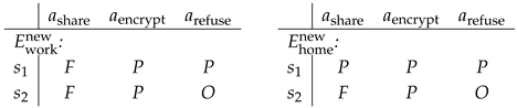
Example 14 (Meta-ethics (level 1): Home vs. Workplace data-sharing rules).  Situations and actions. Let $S=\{s_1=“\mathit{send}\mathit{vacation}\mathit{photos}”,s_2=“\mathit{send}\mathit{customer}\mathit{list}\mathit{to}\mathit{vendor}”\}$ and $A=\{a_{\mathrm{share}},a_{\mathrm{encrypt}},a_{\mathrm{refuse}}\}$.

Two ethical systems on $(S,A)$. Define $E_{\mathrm{home}}=(S,A,{\nu }_{\mathrm{home}})$ and $E_{\mathrm{work}}=(S,A,{\nu }_{\mathrm{work}})$ by the following deontic labels (O=obligatory, P=permissible, F=forbidden):

Home policy $E_{\mathrm{home}}$:

$$\begin{array}{cccc}& a_{\mathrm{share}}& a_{\mathrm{encrypt}}& a_{\mathrm{refuse}}\\ s_1& P& P& P\\ s_2& F& F& O\end{array}$$

Work policy $E_{\mathrm{work}}$:

$$\begin{array}{cccc}& a_{\mathrm{share}}& a_{\mathrm{encrypt}}& a_{\mathrm{refuse}}\\ s_1& F& P& P\\ s_2& F& F& O\end{array}$$

Permissiveness check. From Definition 25,

$${Perm}_{E_{\mathrm{home}}}\left(s_1\right)=\{a_{\mathrm{share}},a_{\mathrm{encrypt}},a_{\mathrm{refuse}}\},{Perm}_{E_{\mathrm{work}}}\left(s_1\right)=\{a_{\mathrm{encrypt}},a_{\mathrm{refuse}}\},$$

$${Perm}_{E_{\mathrm{home}}}\left(s_2\right)=\left\{a_{\mathrm{refuse}}\right\},{Perm}_{E_{\mathrm{work}}}\left(s_2\right)=\left\{a_{\mathrm{refuse}}\right\}.$$

Hence for each $s\in S$, ${Perm}_{E_{\mathrm{work}}}\left(s\right)\subseteq {Perm}_{E_{\mathrm{home}}}\left(s\right)$, i.e., $E_{\mathrm{work}}{⊑}^{\left(1\right)}{E}_{\mathrm{home}}$. All coherence axioms hold (no $O\wedge F$, and some action is always permissible).

Definition 27 (Iterated-Meta-ethics (depth $t\ge 2$)).  Assume level $(t-1)$ objects have been defined. A depth- t Meta-ethics structure is

$${\mathbb{E}}^{\left(t\right)}:=\left(U^{\left(t\right)},{⊑}^{\left(t\right)}\right),$$

where $U^{\left(t\right)}$ is a nonempty set of level-$(t-1)$ Meta-ethics structures. The level-t preorder is lifted by

$$\mathbb{X}{⊑}^{\left(t\right)}\mathbb{Y}:⟺\exists f:U_{\mathbb{X}}\to U_{\mathbb{Y}}\forall E\in U_{\mathbb{X}}:E{⊑}^{(t-1)}f\left(E\right),$$

(12)

where $U_{\mathbb{X}}$ denotes the carrier (set of objects) of $\mathbb{X}$.

Example 15 (Iterated Meta-ethics (level 2): Policy update mapping old → new). Same $S,A$ as above. Consider old and new versions of the two systems:

Old policies.$E_{\mathrm{work}}^{\mathrm{old}}$ as in the previous example. $E_{\mathrm{home}}^{\mathrm{old}}$ as in the previous example.

New policies (strictly more permissive or equal).

(Practically: after adding vetted vendor channels, encrypted transfer becomes permitted.)

Level–1 inclusions. For each $s\in S$,

$${Perm}_{E_{\mathrm{work}}^{\mathrm{old}}}\left(s\right)\subseteq {Perm}_{E_{\mathrm{work}}^{\mathrm{new}}}\left(s\right),{Perm}_{E_{\mathrm{home}}^{\mathrm{old}}}\left(s\right)\subseteq {Perm}_{E_{\mathrm{home}}^{\mathrm{new}}}\left(s\right),$$

so $E_{\mathrm{work}}^{\mathrm{old}}{⊑}^{\left(1\right)}{E}_{\mathrm{work}}^{\mathrm{new}}$ and $E_{\mathrm{home}}^{\mathrm{old}}{⊑}^{\left(1\right)}{E}_{\mathrm{home}}^{\mathrm{new}}$.

Level–2 structures and witness. Let

$$\mathbb{X}=\left(U_{\mathbb{X}},{⊑}^{\left(1\right)}\right),U_{\mathbb{X}}=\{E_{\mathrm{work}}^{\mathrm{old}},E_{\mathrm{home}}^{\mathrm{old}}\},\mathbb{Y}=\left(U_{\mathbb{Y}},{⊑}^{\left(1\right)}\right),U_{\mathbb{Y}}=\{E_{\mathrm{work}}^{\mathrm{new}},E_{\mathrm{home}}^{\mathrm{new}}\}.$$

Define $f:U_{\mathbb{X}}\to U_{\mathbb{Y}}$ by $f\left(E_{\mathrm{work}}^{\mathrm{old}}\right)=E_{\mathrm{work}}^{\mathrm{new}}$ and $f\left(E_{\mathrm{home}}^{\mathrm{old}}\right)=E_{\mathrm{home}}^{\mathrm{new}}$. Then for all $E\in U_{\mathbb{X}}$ we have $E{⊑}^{\left(1\right)}f\left(E\right)$, hence by (12)

$$\mathbb{X}{⊑}^{\left(2\right)}\mathbb{Y}.$$

This models a real-life policy modernization : the level–2 object $\mathbb{Y}$ collects updated (more permissive but controlled) codes that uniformly extend the old ones.

Proposition 7

(Generalization of Meta-ethics). Depth $t=1$ in Definition 27 reproduces Meta-ethics (Definition 26). Hence Iterated-Meta-ethics generalizes Meta-ethics.

Proof. 

For $t=1$ there is no lifting and ${\mathbb{E}}^{\left(1\right)}=(U^{\left(1\right)},{⊑}^{\left(1\right)})$ is exactly Definition 26. □

Lemma 9

(The lifted relation is a preorder). For every $t\ge 2$, ${⊑}^{\left(t\right)}$ defined in (12) is a preorder on $U^{\left(t\right)}$.

Proof. 

Reflexivity: take $f={\mathrm{id}}_{U_{\mathbb{X}}}$; since ${⊑}^{(t-1)}$ is reflexive, $\mathbb{X}{⊑}^{\left(t\right)}\mathbb{X}$. Transitivity: if $\mathbb{X}{⊑}^{\left(t\right)}\mathbb{Y}$ via f and $\mathbb{Y}{⊑}^{\left(t\right)}\mathbb{Z}$ via g , then $E{⊑}^{(t-1)}f\left(E\right){⊑}^{(t-1)}g\left(f\left(E\right)\right)$ for all $E\in U_{\mathbb{X}}$; thus $\mathbb{X}{⊑}^{\left(t\right)}\mathbb{Z}$ via $g\circ f$. □

Theorem 7

(Iterated-Meta-ethics as an Iterated MetaStructure). There exists a single–sorted signature ${\Sigma }_{\mathrm{ME}}$ and a lift ${\mathsf{U}}_{{\Sigma }_{\mathrm{ME}}}$ such that the tower ${\left\{{\mathbb{E}}^{\left(t\right)}\right\}}_{t\ge 1}$ forms an Iterated MetaStructure in the sense of Definition 3. Moreover, depth $t=1$ coincides with Meta-ethics and the lift is isomorphism–invariant.

Proof. Signature and coding. Let ${\Sigma }_{\mathrm{ME}}$ be relational with a single binary symbol $\mathrm{Pre}(·,·)$. A ${\Sigma }_{\mathrm{ME}}$–structure $\mathbf{A}=(X,\mathrm{Pre})$ encodes a Meta-ethics structure by taking X as its carrier (set of objects at that level) and interpreting $\mathrm{Pre}$ as the corresponding preorder ⊑.

Lift. Given a level $(t-1)$ structure ${\mathbf{A}}^{(t-1)}=(U^{(t-1)},{\mathrm{Pre}}^{(t-1)})$, define ${\mathsf{U}}_{{\Sigma }_{\mathrm{ME}}}\left({\mathbf{A}}^{(t-1)}\right)$ to be the structure ${\mathbf{A}}^{\left(t\right)}=(U^{\left(t\right)},{\mathrm{Pre}}^{\left(t\right)})$ whose carrier $U^{\left(t\right)}$ is the set of all level-$(t-1)$ objects and whose relation is the lifted preorder (12). By Lemma 9, ${\mathrm{Pre}}^{\left(t\right)}$ is a preorder.

Isomorphism–invariance. Let $\alpha :(U^{(t-1)},{\mathrm{Pre}}^{(t-1)})\cong (U^{\prime (t-1)},{\mathrm{Pre}}^{\prime (t-1)})$ be an isomorphism (a bijection preserving the preorder). Transporting witnesses f in (12) by $\alpha$ shows that $\alpha$ induces an isomorphism between the lifted structures ${\mathsf{U}}_{{\Sigma }_{\mathrm{ME}}}\left({\mathbf{A}}^{(t-1)}\right)$ and ${\mathsf{U}}_{{\Sigma }_{\mathrm{ME}}}\left({\mathbf{A}}^{\prime (t-1)}\right)$; hence the lift is natural.

Base level. For $t=1$ the encoding is exactly ${\mathbf{A}}^{\left(1\right)}=(U^{\left(1\right)},{⊑}^{\left(1\right)})$, which is Meta-ethics (Definition 26). Therefore the tower ${\left\{{\mathbb{E}}^{\left(t\right)}\right\}}_{t\ge 1}$ is an Iterated MetaStructure with signature ${\Sigma }_{\mathrm{ME}}$. □

Corollary 6

(Sound tower). For every $t\ge 1$, ${\mathbb{E}}^{\left(t\right)}$ is well defined and ${\left\{{\mathbb{E}}^{\left(s\right)}\right\}}_{s=1}^t$ forms an Iterated MetaStructure under ${\mathsf{U}}_{{\Sigma }_{\mathrm{ME}}}$, with a (lifted) permissiveness preorder at each level.

Proof. 

Immediate by induction using Lemma 9 and Theorem 7. □

2.8. Metadata (Data of Data)

A Metadata is structured descriptive information about data objects, defined by schema, attributes, identifiers, and canonical assignments (cf.[64,65,66]). An Iterated-Metadata recursively applies metadata construction, lifting data–about–data into multiple hierarchical levels, preserving identifiers, schemas, and isomorphism invariance.

Definition 28 (Metadata (level 1)).  Let D be a (nonempty) set of data objects . A schema is a pair $\Sigma =(K,Typ)$ where K is a finite set of attribute keys and $Typ:K\to \left\{\mathrm{sets}\right\}$ assigns to each $k\in K$ a value domain $Typ\left(k\right)$. A $\Sigma$–record is a function $r:K\to {⨆}_{k\in K}Typ\left(k\right)$ with $r\left(k\right)\in Typ\left(k\right)$ for all k; write $Rec(\Sigma )$ for the set of all such records.

Fix a distinguished reference key $k_{\mathrm{ref}}\in K$ and an identifier map $id:D\to Typ\left(k_{\mathrm{ref}}\right)$. A metadata assignment on $(D,\Sigma )$ is a map

$$\mu :D⟶Rec(\Sigma )\mathit{satisfying}\forall d\in D:\mu \left(d\right)\left(k_{\mathrm{ref}}\right)=id\left(d\right).$$

The triple ${\mathcal{M}}^{\left(1\right)}=(D,\Sigma ,\mu )$ is called metadata on D.

Definition 29

(Isomorphisms of metadata). Two metadata triples ${\mathcal{M}}^{\left(1\right)}=(D,\Sigma ,\mu )$ and ${\mathcal{M}}^{\prime \left(1\right)}=(D^{\prime },{\Sigma }^{\prime },{\mu }^{\prime })$ are isomorphic , written ${\mathcal{M}}^{\left(1\right)}\cong {\mathcal{M}}^{\prime \left(1\right)}$, if there exist bijections $\alpha :D\to D^{\prime }$ and $\psi :K\to K^{\prime }$ such that

(a) 

${Typ}^{\prime }\left(\psi \left(k\right)\right)=Typ\left(k\right)$ for all $k\in K$ and $\psi \left(k_{\mathrm{ref}}\right)=k_{\mathrm{ref}}^{\prime }$,

(b) 

${id}^{\prime }\left(\alpha \left(d\right)\right)=id\left(d\right)$ for all $d\in D$,

(c) 

for every $d\in D$ and $k\in K$, ${\mu }^{\prime }\left(\alpha \left(d\right)\right)\left(\psi \left(k\right)\right)=\mu \left(d\right)\left(k\right)$.

(I.e. α renames data, ψ renames keys while preserving value domains and the aboutness key, and the records commute with these renamings.)

Definition 30

(Lift to metadata-of-metadata). Given ${\mathcal{M}}^{\left(1\right)}=(D,\Sigma ,\mu )$ with $\Sigma =(K,Typ)$, define its lift$Lift\left({\mathcal{M}}^{\left(1\right)}\right)={\mathcal{M}}^{\left(2\right)}=(D^{\uparrow },{\Sigma }^{\uparrow },{\mu }^{\uparrow })$ by:

$$\begin{array}{cc}\hfill & D^{\uparrow }:=\{(d,\mu \left(d\right)):d\in D\}(\mathit{graph}\mathrm{of}\mu ),\hfill \end{array}$$

(13)

$$\begin{array}{cc}\hfill & K^{\uparrow }:=K\bigsqcup \{k_{\mathrm{ref}}^{\uparrow },k_{\mathrm{prev}}\},{Typ}^{\uparrow }{\upharpoonright }_K\equiv Typ,{Typ}^{\uparrow }\left(k_{\mathrm{ref}}^{\uparrow }\right)=Typ\left(k_{\mathrm{ref}}\right),{Typ}^{\uparrow }\left(k_{\mathrm{prev}}\right)=Rec(\Sigma ),\hfill \end{array}$$

(14)

$$\begin{array}{cc}\hfill & {id}^{\uparrow }:D^{\uparrow }\to {Typ}^{\uparrow }\left(k_{\mathrm{ref}}^{\uparrow }\right),{id}^{\uparrow }(d,\mu \left(d\right)):=id\left(d\right),\hfill \end{array}$$

(15)

$$\begin{array}{cc}\hfill & {\mu }^{\uparrow }:D^{\uparrow }\to Rec\left({\Sigma }^{\uparrow }\right),\mathit{given}\mathit{by}\left\{\begin{array}{cc}{\mu }^{\uparrow }(d,\mu \left(d\right))\left(k\right)=\mu \left(d\right)\left(k\right),\hfill & k\in K,\hfill \\ {\mu }^{\uparrow }(d,\mu \left(d\right))\left(k_{\mathrm{ref}}^{\uparrow }\right)=id\left(d\right),\hfill \\ {\mu }^{\uparrow }(d,\mu \left(d\right))\left(k_{\mathrm{prev}}\right)=\mu \left(d\right).\hfill \end{array}\right.\hfill \end{array}$$

(16)

Then ${\mathcal{M}}^{\left(2\right)}$ is again metadata by Definition 28 (with reference key $k_{\mathrm{ref}}^{\uparrow }$ and identifier ${id}^{\uparrow }$).

Definition 31 (Iterated-Metadata (depth t )).  Let ${\mathcal{M}}^{\left(1\right)}=(D^{\left(1\right)},{\Sigma }^{\left(1\right)},{\mu }^{\left(1\right)})$ be metadata. Define inductively for $t\ge 2$:

$${\mathcal{M}}^{\left(t\right)}:=Lift\left({\mathcal{M}}^{(t-1)}\right)=\left(D^{\left(t\right)},{\Sigma }^{\left(t\right)},{\mu }^{\left(t\right)}\right),$$

using (13)–() at level $t-1$. We call ${\mathcal{M}}^{\left(t\right)}$ Iterated-Metadata of depth t.

Example 16

(From file metadata to metadata-of-metadata). Level 1 (ordinary metadata). Let the data objects be two photos $D=\{d_1,d_2\}$. Use schema $\Sigma =(K,Typ)$ with

$$K=\{k_{\mathrm{ref}}=\mathsf{fileID},\mathsf{date},\mathsf{device},\mathsf{location}\},$$

$$Typ\left(\mathsf{fileID}\right)=\mathsf{Str},Typ\left(\mathsf{date}\right)=\mathsf{Date},Typ\left(\mathsf{device}\right)=\mathsf{Str},Typ\left(\mathsf{location}\right)=\mathsf{Str}.$$

The identifier is $id\left(d\right)=\mathsf{fileID\; of}d$. Define the metadata assignment $\mu :D\to Rec(\Sigma )$ by

$$\begin{array}{cc}\hfill \mu \left(d_1\right):& \mathsf{fileID}=\mathsf{IMG}\_\mathsf{0001}.\mathsf{jpg},\mathsf{date}=\mathsf{2025}\text{-}\mathsf{08}\text{-}\mathsf{20},\mathsf{device}=\mathsf{iPhone}\mathsf{15},\mathsf{location}=\mathsf{Tokyo},\hfill \\ \hfill \mu \left(d_2\right):& \mathsf{fileID}=\mathsf{IMG}\_\mathsf{0002}.\mathsf{jpg},\mathsf{date}=\mathsf{2025}\text{-}\mathsf{08}\text{-}\mathsf{21},\mathsf{device}=\mathsf{Ricoh}\mathsf{GR}\mathsf{III},\mathsf{location}=\mathsf{Yokohama}.\hfill \end{array}$$

Thus ${\mathcal{M}}^{\left(1\right)}=(D,\Sigma ,\mu )$ is metadata in the sense of Definition 28.

Lift (metadata-of-metadata, Level 2). Apply Definition 30:

$$D^{\uparrow }=\{(d_1,\mu \left(d_1\right)),(d_2,\mu \left(d_2\right))\},$$

$$K^{\uparrow }=K\bigsqcup \{k_{\mathrm{ref}}^{\uparrow }={\mathsf{fileID}}^{\uparrow },k_{\mathrm{prev}}\},{Typ}^{\uparrow }{\upharpoonright }_K=Typ,{Typ}^{\uparrow }\left(k_{\mathrm{ref}}^{\uparrow }\right)=\mathsf{Str},{Typ}^{\uparrow }\left(k_{\mathrm{prev}}\right)=Rec(\Sigma ).$$

The lifted identifier is ${id}^{\uparrow }(d,\mu \left(d\right))=id\left(d\right)$. The lifted assignment ${\mu }^{\uparrow }:D^{\uparrow }\to Rec\left({\Sigma }^{\uparrow }\right)$ satisfies, for each $(d,\mu \left(d\right))\in D^{\uparrow }$,

$${\mu }^{\uparrow }(d,\mu \left(d\right))\left(k\right)=\mu \left(d\right)\left(k\right)(k\in K),{\mu }^{\uparrow }(d,\mu \left(d\right))\left(k_{\mathrm{ref}}^{\uparrow }\right)=id\left(d\right),{\mu }^{\uparrow }(d,\mu \left(d\right))\left(k_{\mathrm{prev}}\right)=\mu \left(d\right).$$

Concrete instance (for $d_1$).

$$\begin{array}{cc}& {\mu }^{\uparrow }(d_1,\mu \left(d_1\right))\left(\mathsf{fileID}\right)=\mathsf{IMG}\_\mathsf{0001}.\mathsf{jpg},{\mu }^{\uparrow }(d_1,\mu \left(d_1\right))\left(\mathsf{date}\right)=\mathsf{2025}\text{-}\mathsf{08}\text{-}\mathsf{20},\hfill \\ & {\mu }^{\uparrow }(d_1,\mu \left(d_1\right))\left(\mathsf{device}\right)=\mathsf{iPhone}\mathsf{15},{\mu }^{\uparrow }(d_1,\mu \left(d_1\right))\left(\mathsf{location}\right)=\mathsf{Tokyo},\hfill \\ & {\mu }^{\uparrow }(d_1,\mu \left(d_1\right))\left({\mathsf{fileID}}^{\uparrow }\right)=\mathsf{IMG}\_\mathsf{0001}.\mathsf{jpg},\hfill \\ & {\mu }^{\uparrow }(d_1,\mu \left(d_1\right))\left(k_{\mathrm{prev}}\right)=\mu \left(d_1\right)\left(\mathit{the}\mathit{entire}\mathit{Level}1\mathit{record}\mathit{above}\right).\hfill \end{array}$$

The case for $d_2$ is analogous. Intuitively, each Level 2 record keeps all Level 1 fields, plus (i) a copied identifier for stable linkage and (ii) a pointer to the previous metadata record (provenance). Hence ${\mathcal{M}}^{\left(2\right)}$ is a simple, real-life “metadata-of-metadata” for a phone photo library.

Proposition 8

(Generalization of Metadata). Depth $t=1$ of Definition 31 reproduces ordinary metadata (Definition 28). Hence Iterated-Metadata generalizes Metadata.

Proof. 

Trivial: by definition ${\mathcal{M}}^{\left(1\right)}=(D^{\left(1\right)},{\Sigma }^{\left(1\right)},{\mu }^{\left(1\right)})$ is exactly Definition 28. No lifting is applied at $t=1$. □

Lemma 10 (Naturality (isomorphism invariance) of the lift).  If ${\mathcal{M}}^{\left(1\right)}\cong {\mathcal{M}}^{\prime \left(1\right)}$ via $(\alpha ,\psi )$ as in Definition 29, then $Lift\left({\mathcal{M}}^{\left(1\right)}\right)\cong Lift\left({\mathcal{M}}^{\prime \left(1\right)}\right)$ via

$${\alpha }^{\uparrow }:(d,\mu \left(d\right))\mapsto \left(\alpha \left(d\right),{\mu }^{\prime }\left(\alpha \left(d\right)\right)\right),{\psi }^{\uparrow }:=\psi \bigsqcup \{k_{\mathrm{ref}}^{\uparrow }\mapsto k_{\mathrm{ref}}^{\prime \uparrow },k_{\mathrm{prev}}\mapsto k_{\mathrm{prev}}^{\prime }\}.$$

Proof. 

By (b)–(c) of Definition 29, ${\mu }^{\prime }\left(\alpha \left(d\right)\right)\left(\psi \left(k\right)\right)=\mu \left(d\right)\left(k\right)$ for $k\in K$, and ${id}^{\prime }\left(\alpha \left(d\right)\right)=id\left(d\right)$. Therefore (16) commutes under $({\alpha }^{\uparrow },{\psi }^{\uparrow })$ for all keys, including the two new ones, and (15) is preserved as well. □

Theorem 8

(Iterated-Metadata as an Iterated MetaStructure). There exists a single–sorted signature ${\Sigma }_{\mathrm{MD}}$ and a lift ${\mathsf{U}}_{{\Sigma }_{\mathrm{MD}}}$ such that the tower ${\left\{{\mathcal{M}}^{\left(t\right)}\right\}}_{t\ge 1}$ forms an Iterated MetaStructure (Definition 3). Moreover, depth $t=1$ coincides with Metadata and the lift is isomorphism–invariant.

Proof. Signature and objects. Let ${\Sigma }_{\mathrm{MD}}$ be relational over a single carrier X (tagged union of data, keys, and records) with symbols:

$$\mathrm{Data}\left(x\right),\mathrm{Key}\left(x\right),\mathrm{Val}(x,y)\left(xA\mathrm{record},yA\mathrm{value}\right),$$

$$\mathrm{Has}(x,k,v)\left(\mathrm{record}x\mathrm{has}\mathrm{key}k\mathrm{with}\mathrm{value}v\right),\mathrm{RefKey}\left(k\right),\mathrm{Id}(d,v).$$

A ${\Sigma }_{\mathrm{MD}}$–structure $\mathbf{A}$ encodes a metadata triple $\mathcal{M}=(D,\Sigma ,\mu )$ by taking $X=D\bigsqcup K\bigsqcup Rec(\Sigma )\bigsqcup {\bigcup }_{k}Typ\left(k\right)$, marking sorts with $\mathrm{Data}$/$\mathrm{Key}$, interpreting $\mathrm{Has}$ from $\mu$, and $\mathrm{RefKey}$/$\mathrm{Id}$ from $k_{\mathrm{ref}}$ and id.

Meta–operation (the lift). Define a unary meta–operation ${\Phi }_{\mathrm{lift}}:U\to U$ on the class U of ${\Sigma }_{\mathrm{MD}}$–structures by performing the recipes (13)–(16) at the level of carriers and of the relations $\mathrm{Has},\mathrm{RefKey},\mathrm{Id}$. Concretely: carriers are rebuilt by adding the graph pairs and the two fresh keys; $\mathrm{Has}$ is extended so that each lifted record inherits all original key–value pairs and additionally has entries for $k_{\mathrm{ref}}^{\uparrow }$ (the old identifier) and $k_{\mathrm{prev}}$ (the previous record).

Isomorphism–invariance. If $\alpha :\mathbf{A}\cong {\mathbf{A}}^{\prime }$ is an isomorphism (in particular inducing a pair $(\alpha ,\psi )$ as in Definition 29), then by Lemma 10 the assignments of all relation symbols in ${\Phi }_{\mathrm{lift}}\left(\mathbf{A}\right)$ and ${\Phi }_{\mathrm{lift}}\left({\mathbf{A}}^{\prime }\right)$ agree through the transported $({\alpha }^{\uparrow },{\psi }^{\uparrow })$; hence ${\Phi }_{\mathrm{lift}}$ is natural.

Iterated MetaStructure. Let ${\mathsf{U}}_{{\Sigma }_{\mathrm{MD}}}$ be the functor that sends $\mathbf{A}$ to ${\Phi }_{\mathrm{lift}}\left(\mathbf{A}\right)$ and acts on isomorphisms by transport as above. Iterating ${\mathsf{U}}_{{\Sigma }_{\mathrm{MD}}}$ produces the tower ${\left\{{\mathcal{M}}^{\left(t\right)}\right\}}_{t\ge 1}$ of Definition 31. Depth $t=1$ clearly coincides with ordinary metadata (no lifting applied). □

Corollary 7

(Sound tower). For every $t\ge 1$, ${\mathcal{M}}^{\left(t\right)}$ is well defined, and the family ${\left\{{\mathcal{M}}^{\left(s\right)}\right\}}_{s=1}^t$ forms an Iterated MetaStructure under the isomorphism–invariant lift ${\mathsf{U}}_{{\Sigma }_{\mathrm{MD}}}$.

Proof. 

Immediate by induction on t using Lemma 10 and Theorem 8. □

2.9. Meta-Governance (Governance of Governance)

A Governance system specifies how actors, decision rules, instruments, and processes interact to steer collective actions within institutions. A Meta-Governance structure organizes governance systems, redesigning their modes, instruments, and processes to coordinate failures and reweight steering mechanisms (cf.[67,68,69,70]). An Iterated-Meta-Governance recursively applies meta-governance, layering higher-level coordination over sets of governance structures, ensuring adaptive, hierarchical, multi-level institutional steering.

Definition 32

(Governance System). A governance system is a finite tuple

$$G=(A,D,M,I,P),$$

where

• A is a nonempty finite set of actors;
• D is a set of decision rules and procedures (e.g., voting rules, mandates);
• $M\subseteq \{\mathrm{hierarchy},\mathrm{market},\mathrm{network}\}$ lists the governance modes present;
• I is a set of steering instruments partitioned as $I=I^{\mathrm{auth}}\bigsqcup I^{\mathrm{econ}}\bigsqcup I^{\mathrm{info}}$ (authority, economic, informational instruments);
• P is a set of institutionalized processes (forums, committees, contracts, etc.).

Let $\mathcal{U}$ denote a nonempty set of such governance systems. A (nonnegative) failure functional$\Phi :\mathcal{U}\to {\mathbb{R}}_{\ge 0}$ quantifies coordination deficits, legitimacy problems, or outcome shortfalls.

Definition 33

(Meta-Governance (level 1)). Let $\mathcal{G}$ be the class of governance systems over the fixed $(A,O)$. A Meta-Governance structure is a pair

$${\mathbb{G}}^{\left(1\right)}=\left(U^{\left(1\right)};{⪯}^{\left(1\right)},{\mathrm{Req}}^{\left(1\right)},{\mathrm{Cov}}^{\left(1\right)},{\mathrm{Comp}}^{\left(1\right)}\right),$$

where $U^{\left(1\right)}\subseteq \mathcal{G}$ is nonempty and

• ${⪯}^{\left(1\right)}$ is a preorder on $U^{\left(1\right)}$ defined componentwise by

  $$G{⪯}^{\left(1\right)}H:⟺{\mathrm{Req}}_G\subseteq {\mathrm{Req}}_H\mathrm{and}{\mathrm{Cov}}_G\subseteq {\mathrm{Cov}}_H;$$
• ${\mathrm{Req}}^{\left(1\right)}(G,a,o):={\mathrm{Req}}_G(a,o)$ and ${\mathrm{Cov}}^{\left(1\right)}(G,a,o):={\mathrm{Cov}}_G(a,o)$;
• ${\mathrm{Comp}}^{\left(1\right)}(G,a)$ is the compliance predicate of G from Definition .

This satisfies meta-monotonicity :

$$G{⪯}^{\left(1\right)}H\wedge {\mathrm{Req}}^{\left(1\right)}(G,a,o)\Rightarrow {\mathrm{Req}}^{\left(1\right)}(H,a,o),G{⪯}^{\left(1\right)}H\wedge {\mathrm{Cov}}^{\left(1\right)}(G,a,o)\Rightarrow {\mathrm{Cov}}^{\left(1\right)}(H,a,o),$$

and in particular

$$G{⪯}^{\left(1\right)}H\wedge {\mathrm{Comp}}^{\left(1\right)}(G,a)\Rightarrow {\mathrm{Comp}}^{\left(1\right)}(H,a).$$

Example 17

(Concrete level-1 Meta-Governance with numbers). Let

$$A=\{\mathbf{PII},\mathbf{Health}\}$$

,

$$O=\{\mathbf{Enc},\mathbf{Consent},\mathbf{Retention}\}$$

. Write rows in the order $(\mathbf{PII},\mathbf{Health})$ and columns $(\mathbf{Enc},\mathbf{Consent},\mathbf{Retention})$. Consider $G_1,G_2\in \mathcal{G}$ with

$${\mathrm{Req}}_{G_1}=\left[\begin{array}{ccc}1& 0& 1\\ 1& 1& 1\end{array}\right],$$

$${\mathrm{Cov}}_{G_1}=\left[\begin{array}{ccc}1& 0& 1\\ 1& 0& 1\end{array}\right],$$

$$r_{G_1}\left(\mathbf{PII}\right)=0.02,r_{G_1}\left(\mathbf{Health}\right)=0.20,{\kappa }_{G_1}=3.0;$$

$${\mathrm{Req}}_{G_2}=\left[\begin{array}{ccc}1& 1& 1\\ 1& 1& 1\end{array}\right],$$

$${\mathrm{Cov}}_{G_2}=\left[\begin{array}{ccc}1& 1& 1\\ 1& 1& 1\end{array}\right],$$

$$r_{G_2}\left(\mathbf{PII}\right)=0.01,r_{G_2}\left(\mathbf{Health}\right)=0.05,{\kappa }_{G_2}=4.5.$$

Then ${\mathrm{Req}}_{G_1}\subseteq {\mathrm{Req}}_{G_2}$ and ${\mathrm{Cov}}_{G_1}\subseteq {\mathrm{Cov}}_{G_2}$, hence $G_1{⪯}^{\left(1\right)}{G}_2$. Compliance:

$${\mathrm{Comp}}_{G_1}\left(\mathbf{PII}\right)=1,{\mathrm{Comp}}_{G_1}\left(\mathbf{Health}\right)=0;$$

$${\mathrm{Comp}}_{G_2}\left(\mathbf{PII}\right)={\mathrm{Comp}}_{G_2}\left(\mathbf{Health}\right)=1.$$

The risk profile respects (G1) and (G2): adding coverage (from $G_1$ to $G_2$) weakly decreases risk componentwise: $0.01\le 0.02$ and $0.05\le 0.20$.

Definition 34

(Iterated-Meta-Governance (depth t )). For $t\ge 2$, a depth- t Iterated-Meta-Governance structure is a tuple

$${\mathbb{G}}^{\left(t\right)}=\left(U^{\left(t\right)};{⪯}^{\left(t\right)},{\mathrm{Req}}^{\left(t\right)},{\mathrm{Cov}}^{\left(t\right)},{\mathrm{Comp}}^{\left(t\right)}\right),$$

where $U^{\left(t\right)}$ is a nonempty set of depth-$(t-1)$ objects and the lift is:

$$\begin{array}{cccc}\hfill & \mathbf{Order}\mathbf{lift}:\hfill & \hfill & \mathfrak{X}{⪯}^{\left(t\right)}\mathfrak{Y}:⟺\exists f:U_{\mathfrak{X}}\to U_{\mathfrak{Y}}\forall G\in U_{\mathfrak{X}},G{⪯}^{(t-1)}f\left(G\right).\hfill \end{array}$$

(17)

$$\begin{array}{cccc}\hfill & \mathbf{Requirement}\mathbf{lift}\left(\mathbf{OR}\right):\hfill & \hfill & {\mathrm{Req}}^{\left(t\right)}(\mathfrak{X},a,o):⟺\exists G\in U_{\mathfrak{X}}:{\mathrm{Req}}^{(t-1)}(G,a,o).\hfill \end{array}$$

(18)

$$\begin{array}{cccc}\hfill & \mathbf{Coverage}\mathbf{lift}\left(\mathbf{AND}\right):\hfill & \hfill & {\mathrm{Cov}}^{\left(t\right)}(\mathfrak{X},a,o):⟺\forall G\in U_{\mathfrak{X}}:{\mathrm{Cov}}^{(t-1)}(G,a,o).\hfill \end{array}$$

(19)

Set ${\mathrm{Comp}}^{\left(t\right)}(\mathfrak{X},a)$ by the same formula as at base level:

$${\mathrm{Comp}}^{\left(t\right)}(\mathfrak{X},a):=\left[\forall o\in O,{\mathrm{Req}}^{\left(t\right)}(\mathfrak{X},a,o)\Rightarrow {\mathrm{Cov}}^{\left(t\right)}(\mathfrak{X},a,o)\right].$$

Proposition 9

(Generalization of Meta-Governance). Depth $t=1$ in Definition 34 reduces to Meta-Governance (Definition 33). For $t=0$ one has only base governance systems.

Proof. 

At $t=1$ the lifted clauses are identities: no f is required beyond $f=\mathrm{id}$ and (18)–(19) collapse to the base relations. For $t=0$, the meta-level disappears. □

Lemma 11

(Axioms preserved by the lift). Fix $t\ge 2$. If ${⪯}^{(t-1)}$ is a preorder and the meta-monotonicities of Definition 33 hold at depth $t-1$, then:

(a) 

${⪯}^{\left(t\right)}$ is a preorder;

(b) 

${\mathrm{Req}}^{\left(t\right)}$ is monotone along ${⪯}^{\left(t\right)}$;

(c) 

${\mathrm{Cov}}^{\left(t\right)}$ is monotone along ${⪯}^{\left(t\right)}$;

(d) 

${\mathrm{Comp}}^{\left(t\right)}$ is monotone along ${⪯}^{\left(t\right)}$.

Proof. (a) Reflexivity is witnessed by $f=\mathrm{id}$. Transitivity: if $\mathfrak{X}{⪯}^{\left(t\right)}\mathfrak{Y}$ via f and $\mathfrak{Y}{⪯}^{\left(t\right)}\mathfrak{Z}$ via g , then $g\circ f$ witnesses $\mathfrak{X}{⪯}^{\left(t\right)}\mathfrak{Z}$ because ${⪯}^{(t-1)}$ is transitive.

(b) Suppose $\mathfrak{X}{⪯}^{\left(t\right)}\mathfrak{Y}$ via f and ${\mathrm{Req}}^{\left(t\right)}(\mathfrak{X},a,o)$. Choose $G\in U_{\mathfrak{X}}$ with ${\mathrm{Req}}^{(t-1)}(G,a,o)$. Then $G{⪯}^{(t-1)}f\left(G\right)$ and level-$(t-1)$ monotonicity give ${\mathrm{Req}}^{(t-1)}(f\left(G\right),a,o)$, hence by (18) we get ${\mathrm{Req}}^{\left(t\right)}(\mathfrak{Y},a,o)$.

(c) Suppose $\mathfrak{X}{⪯}^{\left(t\right)}\mathfrak{Y}$ via f and ${\mathrm{Cov}}^{\left(t\right)}(\mathfrak{X},a,o)$. Then for all $G\in U_{\mathfrak{X}}$, ${\mathrm{Cov}}^{(t-1)}(G,a,o)$. By monotonicity at $t-1$ and $G{⪯}^{(t-1)}f\left(G\right)$ we have ${\mathrm{Cov}}^{(t-1)}(f\left(G\right),a,o)$ for all G , so by (19), ${\mathrm{Cov}}^{\left(t\right)}(\mathfrak{Y},a,o)$.

(d) Combine (b) and (c) with the definition of ${\mathrm{Comp}}^{\left(t\right)}$. □

Example 18

(Worked depth-2 check using Example 17). Let $\mathfrak{X}$ be the level-1 object containing only $G_1$ and $\mathfrak{Y}$ the one containing only $G_2$. Then $f\left(G_1\right)=G_2$ witnesses $\mathfrak{X}{⪯}^{\left(2\right)}\mathfrak{Y}$.

Lifted requirement (OR):${\mathrm{Req}}^{\left(2\right)}(\mathfrak{X},\mathbf{PII},\mathbf{Enc})=1$ because ${\mathrm{Req}}^{\left(1\right)}(G_1,\mathbf{PII},\mathbf{Enc})=1$; likewise for $\mathfrak{Y}$.

Lifted coverage (AND):${\mathrm{Cov}}^{\left(2\right)}(\mathfrak{X},\mathbf{Health},\mathbf{Consent})=0$ since ${\mathrm{Cov}}^{\left(1\right)}(G_1,\mathbf{Health},\mathbf{Consent})=0$; while ${\mathrm{Cov}}^{\left(2\right)}(\mathfrak{Y},\mathbf{Health},\mathbf{Consent})=1$.

Lifted compliance:${\mathrm{Comp}}^{\left(2\right)}(\mathfrak{X},\mathbf{PII})=1$, ${\mathrm{Comp}}^{\left(2\right)}(\mathfrak{X},\mathbf{Health})=0$, ${\mathrm{Comp}}^{\left(2\right)}(\mathfrak{Y},\mathbf{PII})={\mathrm{Comp}}^{\left(2\right)}(\mathfrak{Y},\mathbf{Health})=1$. Thus compliance is monotone along $\mathfrak{X}{⪯}^{\left(2\right)}\mathfrak{Y}$, in line with Lemma 11(d).

Theorem 9

(Iterated Meta-Governance is an Iterated MetaStructure). There exists a single-sorted signature ${\Sigma }_{\mathrm{MG}}$ and a lift ${\mathsf{U}}_{{\Sigma }_{\mathrm{MG}}}$ such that the family ${\left\{{\mathbb{G}}^{\left(t\right)}\right\}}_{t\ge 1}$ of Definitions 33–34 forms an Iterated MetaStructure in the sense of Definition 3. Moreover, depth $t=1$ coincides with Meta-Governance and the lift is isomorphism-invariant.

Proof. Coding. Let ${\Sigma }_{\mathrm{MG}}$ have unary predicates $G\left(x\right)$, $A\left(x\right)$, $O\left(x\right)$ tagging governance objects , assets , and obligations , and relation symbols

$$\mathrm{Pre}(x,y)(G\times G),\mathrm{Req}(x,a,o)(G\times A\times O),\mathrm{Cov}(x,a,o)(G\times A\times O).$$

A Meta-Governance structure ${\mathbb{G}}^{\left(t\right)}$ is represented by a ${\Sigma }_{\mathrm{MG}}$–structure whose carrier is the disjoint union of (tags of) $U^{\left(t\right)}$, A , O , with $\mathrm{Pre},\mathrm{Req},\mathrm{Cov}$ interpreted as ${⪯}^{\left(t\right)},{\mathrm{Req}}^{\left(t\right)},{\mathrm{Cov}}^{\left(t\right)}$ (compliance is definable from $\mathrm{Req}$ and $\mathrm{Cov}$).

Lift. Given a level-$(t-1)$ structure, define ${\mathsf{U}}_{{\Sigma }_{\mathrm{MG}}}$ by replacing governance-points with depth-$(t-1)$ objects and interpreting $\mathrm{Pre},\mathrm{Req},\mathrm{Cov}$ by the lifted clauses (17)–(19). This is a purely relational instance of Definition 2.

Verification. By Lemma 11, $\mathrm{Pre}$ is a preorder and $\mathrm{Req}$, $\mathrm{Cov}$ (hence $\mathrm{Comp}$) are monotone along $\mathrm{Pre}$ at every height; these properties are preserved by ${\mathsf{U}}_{{\Sigma }_{\mathrm{MG}}}$ because the lift only composes witnessing maps f and quantifies over elements of $U^{\left(t\right)}$ (no choice of representatives is involved). Isomorphism-invariance follows since the definitions use only first-order formulas built from the relations and bounded quantifiers over the carriers, hence are stable under any isomorphism of the lower-level structures.

Depth 1. When $t=1$ there is no lifting and the encoded structure is exactly Definition 33. □

Corollary 8

(Soundness of the governance tower). For every $t\ge 1$, the object ${\mathbb{G}}^{\left(t\right)}$ is well defined and ${\left\{{\mathbb{G}}^{\left(s\right)}\right\}}_{s=1}^t$ forms an Iterated MetaStructure under ${\mathsf{U}}_{{\Sigma }_{\mathrm{MG}}}$.

Proof. 

Immediate from Lemma 11 and Theorem 9 by induction on t . □

3. Conclusion

This paper examined whether concepts such as Ontology, Computing, Puzzle, Logic, Ethics, Data, and Governance can be systematically extended within the framework of MetaStructures and Iterated MetaStructures. Since the present work has been limited to theoretical considerations, it is hoped that future studies will carry out quantitative analyses employing these ideas.

In addition, we intend to explore further extensions using Rough Sets [71,72,73], Soft Sets [74,75,76], HyperSoft Sets [77,78,79], TreeSoft Sets [80,81,82], Fuzzy Sets [83,84,85,86], HyperFuzzy Sets [28,87,88], Intuitionistic Fuzzy Sets [89,90], Neutrosophic Sets [91,92,93], Quadripartitioned Neutrosophic Sets [94,95], Triple-Valued Neutrosophic Sets [96,97,98], and Plithogenic Sets [99,100], among others.

References

- Fujita, T.; Smarandache, F. A Unified Framework for U -Structures and Functorial Structure: Managing Super, Hyper, SuperHyper, Tree, and Forest Uncertain Over/Under/Off Models. Neutrosophic Sets and Systems 2025, 91, 337–380. [Google Scholar]
- Fujita, T. How to Represent A→ B →⋯→ Z: From Curried Functions and Hyperfunctions to Curried Structures and Hyperstructures, and More, 2025. [CrossRef]
- Hausdorff, F. Set theory ; Vol. 119, American Mathematical Soc., 2021.
- Jech, T. Set theory: The third millennium edition, revised and expanded ; Springer, 2003.
- Panti, G. Multi-valued logics. In Quantified representation of uncertainty and imprecision ; Springer, 1998; pp. 25–74.
- Jaynes, E.T.; Grandy, T.B.; Smith, R.; Loredo, T.; Tribus, M.; Skilling, J.; Bretthorst, G.L. Probability theory: the logic of science. The Mathematical Intelligencer 2005, 27, 83. [Google Scholar] [CrossRef]
- Kingman, J.F.C.; Feller, W. An Introduction to Probability Theory and its Applications. Biometrika 1958, 130, 430–430. [Google Scholar]
- Chen, J.; Ye, J.; Du, S. Scale Effect and Anisotropy Analyzed for Neutrosophic Numbers of Rock Joint Roughness Coefficient Based on Neutrosophic Statistics. Symmetry 2017, 9, 208. [Google Scholar] [CrossRef]
- Smarandache, F. Plithogeny, plithogenic set, logic, probability, and statistics. arXiv preprint arXiv:1808.03948 2018.
- Lenz, R.; Bovik, A.C. Group Theory. 2007.
- Burde, D. Group Theory. Computers, Rigidity, and Moduli 2019.
- Wisbauer, R. Foundations of module and ring theory; Routledge, 2018.
- Stenstrom, B. Rings of quotients: an introduction to methods of ring theory ; Vol. 217, Springer Science & Business Media, 2012.
- Dehghan, O.; Ameri, R.; Aliabadi, H.E. Some results on hypervector spaces. Italian Journal of Pure and Applied Mathematics 2019, 41, 23–41. [Google Scholar]
- Sameena, K.; et al. FUZZY MATROIDS FROM FUZZY VECTOR SPACES. South East Asian Journal of Mathematics and Mathematical Sciences 2021, 17, 381–390. [Google Scholar]
- Hatip, A.; Olgun, N.; et al. On the Concepts of Two-Fold Fuzzy Vector Spaces and Algebraic Modules. Journal of Neutrosophic and Fuzzy Systems 2023, 7, 46–52. [Google Scholar]
- Diestel, R. Graph theory 3rd ed. Graduate texts in mathematics 2005, 173, 12. [Google Scholar]
- Gross, J.L.; Yellen, J.; Anderson, M. Graph theory and its applications ; Chapman and Hall/CRC, 2018.
- Diestel, R. Graph theory ; Springer (print edition); Reinhard Diestel (eBooks), 2024.
- Smarandache, F. Extension of HyperGraph to n-SuperHyperGraph and to Plithogenic n-SuperHyperGraph, and Extension of HyperAlgebra to n-ary (Classical-/Neutro-/Anti-) HyperAlgebra ; Infinite Study, 2020.
- Hou, Z. Automata Theory and Formal Languages. Texts in Computer Science 2021. [Google Scholar]
- Bonakdarpour, B.; Sheinvald, S. Automata for hyperlanguages. arXiv preprint arXiv:2002.09877 2020.
- Kovach, N.; Gibson, A.S.; Lamont, G.B. Hypergame Theory: A Model for Conflict, Misperception, and Deception. 2015.
- House, J.T.; Cybenko, G.V. Hypergame theory applied to cyber attack and defense. In Proceedings of the Defense + Commercial Sensing, 2010.
- Oguz, G.; Davvaz, B. Soft topological hyperstructure. J. Intell. Fuzzy Syst. 2021, 40, 8755–8764. [Google Scholar] [CrossRef]
- Vougioukli, S. Helix hyperoperation in teaching research. Science & Philosophy 2020, 8, 157–163. [Google Scholar]
- Vougioukli, S. HELIX-HYPEROPERATIONS ON LIE-SANTILLI ADMISSIBILITY. Algebras Groups and Geometries 2023. [Google Scholar] [CrossRef]
- Fujita, T. Advancing Uncertain Combinatorics through Graphization, Hyperization, and Uncertainization: Fuzzy, Neutrosophic, Soft, Rough, and Beyond ; Biblio Publishing, 2025.
- Smarandache, F. Foundation of SuperHyperStructure & Neutrosophic SuperHyperStructure. Neutrosophic Sets and Systems 2024, 63, 21. [Google Scholar]
- Smarandache, F. SuperHyperFunction, SuperHyperStructure, Neutrosophic SuperHyperFunction and Neutrosophic SuperHyperStructure: Current understanding and future directions ; Infinite Study, 2023.
- Das, A.K.; Das, R.; Das, S.; Debnath, B.K.; Granados, C.; Shil, B.; Das, R. A Comprehensive Study of Neutrosophic SuperHyper BCI-Semigroups and their Algebraic Significance. Transactions on Fuzzy Sets and Systems 2025, 8, 80. [Google Scholar]
- Fujita, T. Chemical Hyperstructures, SuperHyperstructures, and SHv-Structures: Toward a Generalized Framework for Hierarchical Chemical Modeling. ChemRxiv 2025. [Google Scholar] [CrossRef]
- Fujita, T. MetaStructure, Meta-HyperStructure, and Meta-SuperHyperStructure, 2025. Preprint. [CrossRef]
- Fujita, T. MetaHyperGraphs, MetaSuperHyperGraphs, and Iterated MetaGraphs: Modeling Graphs of Graphs, Hypergraphs of Hypergraphs, Superhypergraphs of Superhypergraphs, and Beyond, 2025. [CrossRef]
- Fujita, T. Meta-Fuzzy Graph, Meta-Neutrosophic Graph, Meta-Digraph, and Meta-MultiGraph with some applications 2025.
- Fujita, T. MetaFuzzy, MetaNeutrosophic, MetaSoft, and MetaRough Set 2025.
- Smith, B. Ontology. In The furniture of the world ; Brill, 2012; pp. 47–68.
- Guarino, N.; Oberle, D.; Staab, S. What is an ontology? Handbook on ontologies 2009, pp. 1–17.
- Berto, F.; Plebani, M. Ontology and metaontology: A contemporary guide; Bloomsbury Publishing, 2015.
- Chalmers, D.; Manley, D.; Wasserman, R. Metametaphysics: New essays on the foundations of ontology ; Oxford University Press, 2009.
- Dodd, J. Adventures in the metaontology of art: local descriptivism, artefacts and dreamcatchers. Philosophical Studies 2013, 165, 1047–1068. [Google Scholar] [CrossRef]
- Smarr, L.; Catlett, C.E. Metacomputing. Communications of the ACM 1992, 35, 44–52. [Google Scholar] [CrossRef]
- Resch, M.M. Metacomputing in a high performance computing center. In Proceedings of the Proceedings 2000. International Workshop on Parallel Processing. IEEE, 2000, pp. 165–172.
- Foster, I.; Geisler, J.; Kesselman, C.; Tuecke, S. Multimethod communication for high-performance metacomputing applications. In Proceedings of the Proceedings of the 1996 ACM/IEEE Conference on Supercomputing, 1996, pp. 41–es.
- Eickermann, T.; Henrichs, J.; Resch, M.; Stoy, R.; Völpel, R. Metacomputing in gigabit environments: Networks, tools, and applications. Parallel Computing 1998, 24, 1847–1872. [Google Scholar] [CrossRef]
- Wolfson, H.; Schonberg, E.; Kalvin, A.; Lamdan, Y. Solving jigsaw puzzles by computer. Annals of Operations Research 1988, 12, 51–64. [Google Scholar] [CrossRef]
- Makridis, M.; Papamarkos, N. A new technique for solving puzzles. IEEE Transactions on Systems, Man, and Cybernetics, Part B (Cybernetics) 2009, 40, 789–797. [Google Scholar] [CrossRef] [PubMed]
- Kirsner, J.B. Ulcerative Colitis: Puzzles within Puzzles, 1970.
- Netzer, A. An Annotated Bibliography ; Institute of Asian and African Studies, the Hebrew University of Jerusalem, 2004.
- McKenzie, D.F. Bibliography and the Sociology of Texts ; Cambridge University Press, 1999.
- Hendry, D.G.; Jenkins, J.; McCarthy, J.F. Collaborative bibliography. Information Processing & Management 2006, 42, 805–825. [Google Scholar] [CrossRef]
- Bond, D.F. A World Bibliography of Bibliographies and of Bibliographical Catalogues, Calendars, Abstracts, Digests, Indexes, and the Like, 1957.
- Turchin, P. Does population ecology have general laws? Oikos 2001, 94, 17–26. [Google Scholar] [CrossRef]
- Kritzer, J.P.; Sale, P.F. Marine metapopulations ; Elsevier, 2010.
- Grimm, V.; Reise, K.; Strasser, M. Marine metapopulations: a useful concept? Helgoland Marine Research 2003, 56, 222–228. [Google Scholar] [CrossRef]
- Keymer, J.E.; Galajda, P.; Muldoon, C.; Park, S.; Austin, R.H. Bacterial metapopulations in nanofabricated landscapes. Proceedings of the National Academy of Sciences 2006, 103, 17290–17295. [Google Scholar] [CrossRef]
- Janssen, A.; van Gool, E.; Lingeman, R.; Jacas, J.; van de Klashorst, G. Metapopulation dynamics of a persisting predator–prey system in the laboratory: time series analysis. Experimental & Applied Acarology 1997, 21, 415–430. [Google Scholar]
- Hunter, G. Metalogic: An introduction to the metatheory of standard first order logic ; Univ of California Press, 1973.
- Hunter, G. An Introduction to the Metatheory of Standard First Order Logic. Metalogic. Palgrave Macmillan UK, London 1971.
- Woleński, J. On the Relation of Logic to Metalogic. In Proceedings of the Philosophy of Logic and Mathematics: Proceedings of the 41st International Ludwig Wittgenstein Symposium. Walter de Gruyter GmbH & Co KG, 2019, Vol. 27, p. 91.
- Baofu, P. Beyond ethics to post-ethics: A preface to a new theory of morality and immorality ; IAP, 2011.
- Berggren, N. Does ethical subjectivism pose a challenge to classical liberalism? Reason Papers 2004, 27, 69–86. [Google Scholar]
- Couture, J.; Nielsen, K. Introduction: The ages of metaethics. Canadian Journal of Philosophy Supplementary Volume 1995, 21, 1–30. [Google Scholar] [CrossRef]
- Hayashi, T.; Ohsawa, Y. Understanding the structural characteristics of data platforms using metadata and a network approach. IEEE access 2020, 8, 35469–35481. [Google Scholar] [CrossRef]
- Li, Z.; Wen, J.; Zhang, X.; Wu, C.; Li, Z.; Liu, L. ClinData Express–a metadata driven clinical research data management system for secondary use of clinical data. In Proceedings of the AMIA annual symposium proceedings, 2012, Vol. 2012, p. 552.
- Kurokawa, S.; Iwaki, Y.; Miyaho, N. Study on the distributed data sharing mechanism with a mutual authentication and meta database technology. In Proceedings of the 2007 Asia-Pacific Conference on Communications. IEEE, 2007, pp. 215–218.
- Gjaltema, J.; Biesbroek, R.; Termeer, K. From government to governance… to meta-governance: a systematic literature review. Public management review 2020, 22, 1760–1780. [Google Scholar] [CrossRef]
- Jessop, B. From governance to governance failure and from multi-level governance to multi-scalar meta-governance. In The disoriented state: Shifts in governmentality, territoriality and governance ; Springer, 2009; pp. 79–98.
- Rayner, J. The past and future of governance studies: From governance to meta-governance? In Varieties of Governance: Dynamics, Strategies, Capacities ; Springer, 2015; pp. 235–254.
- Müller, R. From network governance to metagovernance. In Research Handbook on the Governance of Projects ; Edward Elgar Publishing, 2023; pp. 366–378.
- Pawlak, Z. Rough sets. International journal of computer & information sciences 1982, 11, 341–356. [Google Scholar]
- Pawlak, Z. Rough sets: Theoretical aspects of reasoning about data ; Vol. 9, Springer Science & Business Media, 2012.
- Broumi, S.; Smarandache, F.; Dhar, M. Rough neutrosophic sets. Infinite Study 2014, 32, 493–502. [Google Scholar]
- Jose, J.; George, B.; Thumbakara, R.K. Soft directed graphs, their vertex degrees, associated matrices and some product operations. New Mathematics and Natural Computation 2023, 19, 651–686. [Google Scholar] [CrossRef]
- Jose, J.; George, B.; Thumbakara, R.K. Soft Graphs: A Comprehensive Survey. New Mathematics and Natural Computation 2024, pp. 1–52.
- Molodtsov, D. Soft set theory-first results. Computers & mathematics with applications 1999, 37, 19–31. [Google Scholar]
- Salamai, A.A. A SuperHyperSoft Framework for Comprehensive Risk Assessment in Energy Projects. Neutrosophic Sets and Systems 2025, 77, 614–624. [Google Scholar]
- Smarandache, F. Extension of soft set to hypersoft set, and then to plithogenic hypersoft set. Neutrosophic sets and systems 2018, 22, 168–170. [Google Scholar]
- Musa, S.Y.; Mohammed, R.A.; Asaad, B.A. N-hypersoft sets: An innovative extension of hypersoft sets and their applications. Symmetry 2023, 15, 1795. [Google Scholar] [CrossRef]
- Myvizhi, M.; A Metwaly, A.; Ali, A.M. TreeSoft Approach for Refining Air Pollution Analysis: A Case Study. Neutrosophic Sets and Systems 2024, 68, 17. [Google Scholar]
- Fujita, T. Smarandache. Quantum-treesoft set and quantum-forestsoft set. Journal of Analysis and Applications 2025, 23, 87–116. [Google Scholar]
- Smarandache, F. TreeSoft Set vs. HyperSoft Set and Fuzzy-Extensions of TreeSoft Sets. HyperSoft Set Methods in Engineering 2024. [Google Scholar] [CrossRef]
- Zadeh, L.A. Fuzzy sets. Information and control 1965, 8, 338–353. [Google Scholar] [CrossRef]
- Al-Hawary, T. Complete fuzzy graphs. International Journal of Mathematical Combinatorics 2011, 4, 26. [Google Scholar]
- Mordeson, J.N.; Nair, P.S. Fuzzy graphs and fuzzy hypergraphs ; Vol. 46, Physica, 2012.
- Rosenfeld, A. Fuzzy graphs. In Fuzzy sets and their applications to cognitive and decision processes ; Elsevier, 1975; pp. 77–95.
- Ghosh, J.; Samanta, T.K. Hyperfuzzy sets and hyperfuzzy group. Int. J. Adv. Sci. Technol 2012, 41, 27–37. [Google Scholar]
- Jun, Y.B.; Song, S.Z.; Kim, S.J. Distances between hyper structures and length fuzzy ideals of BCK/BCI-algebras based on hyper structures. Journal of Intelligent & Fuzzy Systems 2018, 35, 2257–2268. [Google Scholar]
- Atanassov, K.T. Circular intuitionistic fuzzy sets. Journal of Intelligent & Fuzzy Systems 2020, 39, 5981–5986. [Google Scholar] [CrossRef]
- Das, S.; Kar, S. Intuitionistic multi fuzzy soft set and its application in decision making. In Proceedings of the Pattern Recognition and Machine Intelligence: 5th International Conference, PReMI 2013, Kolkata, India, December 10-14, 2013. Proceedings 5. Springer, 2013, pp. 587–592.
- Smarandache, F.; Jdid, M. An Overview of Neutrosophic and Plithogenic Theories and Applications 2023.
- Broumi, S.; Talea, M.; Bakali, A.; Smarandache, F. Single valued neutrosophic graphs. Journal of New theory 2016, 86–101. [Google Scholar]
- Zhu, S. Neutrosophic n-SuperHyperNetwork: A New Approach for Evaluating Short Video Communication Effectiveness in Media Convergence. Neutrosophic Sets and Systems 2025, 85, 1004–1017. [Google Scholar]
- Radha, R.; Mary, A.S.A.; Smarandache, F. Quadripartitioned neutrosophic pythagorean soft set. International Journal of Neutrosophic Science (IJNS) 2021, 14, 11. [Google Scholar] [CrossRef]
- Hussain, S.; Hussain, J.; Rosyida, I.; Broumi, S. Quadripartitioned neutrosophic soft graphs. In Handbook of Research on Advances and Applications of Fuzzy Sets and Logic ; IGI Global, 2022; pp. 771–795.
- Fujita, T. Triple-Valued Neutrosophic Set, Quadruple-Valued Neutrosophic Set, Quintuple-Valued Neutrosophic Set, and Double-valued Indetermsoft Set. Neutrosophic Systems with Applications 2025, 25, 3. [Google Scholar] [CrossRef]
- Wang, H. Professional Identity Formation in Traditional Chinese Medicine Students: An Educational Perspective using Triple-Valued Neutrosophic Set. Neutrosophic Sets and Systems 2025, 88, 83–92. [Google Scholar]
- Jia, J. Triple-Valued Neutrosophic Off for Public Digital Cultural Service Level Evaluation in Craft and Art Museums. Neutrosophic Sets and Systems 2025, 88, 690–698. [Google Scholar]
- Singh, P.K. Intuitionistic Plithogenic Graph ; Infinite Study, 2022.
- Sultana, F.; Gulistan, M.; Ali, M.; Yaqoob, N.; Khan, M.; Rashid, T.; Ahmed, T. A study of plithogenic graphs: applications in spreading coronavirus disease (COVID-19) globally. Journal of ambient intelligence and humanized computing 2023, 14, 13139–13159. [Google Scholar] [CrossRef] [PubMed]
Disclaimer/Publisher’s Note: The statements, opinions and data contained in all publications are solely those of the individual author(s) and contributor(s) and not of MDPI and/or the editor(s). MDPI and/or the editor(s) disclaim responsibility for any injury to people or property resulting from any ideas, methods, instructions or products referred to in the content. |
© 2025 by the authors. Licensee MDPI, Basel, Switzerland. This article is an open access article distributed under the terms and conditions of the Creative Commons Attribution (CC BY) license (http://creativecommons.org/licenses/by/4.0/).
Copyright: This open access article is published under a Creative Commons CC BY 4.0 license, which permit the free download, distribution, and reuse, provided that the author and preprint are cited in any reuse.