
Submitted:
01 September 2025
Posted:
02 September 2025
You are already at the latest version
Abstract
The detection of astronomical transient events—such as supernovae, gamma-ray bursts, and stellar flares—has become increasingly vital in astrophysics due to their association with extreme cosmic processes. However, identifying these short-lived phenomena within massive sky survey datasets, like those from the GOTO project, poses major challenges for traditional analysis methods. This study proposes a Deep Learning approach using Convolutional Neural Networks (CNNs) to improve transient classification. By leveraging Transfer Learning and Fine-Tuning on pre-trained ImageNet models, the system adapts to the specific features of astronomical imagery. Data Augmentation techniques—including rotation, flipping, and noise injection—are employed to enhance dataset diversity, while Dropout and varying Batch Sizes are explored to reduce overfitting and improve generalization. To further boost performance, Ensemble Learning strategies such as Soft Voting and Weighted Voting are implemented, combining multiple CNN models for more robust predictions. The results demonstrate that this integrated approach significantly enhances the accuracy and reliability of transient detection, offering a scalable solution for real-time applications in large-scale surveys like GOTO.
Keywords:
astronomical transients
; convolutional neural networks (CNNs)
; transfer learning
; fine-tuning
; ensemble learning
; optical transient detection
; biomimetics
; bio-inspired computing
1. Introduction
The discovery of astronomical transient events—such as supernovae, gamma-ray bursts, and stellar flares—has become a central focus in modern astrophysics. These phenomena are signatures of high-energy cosmic processes, including neutron star mergers, black hole collisions, and the collapse of massive stars. These signals not only reveal the mechanisms behind the origin of matter and energy but also reflect fundamental physical laws that cannot be replicated in terrestrial laboratories[1,2]. However, identifying and classifying such events in practice poses considerable challenges, especially in the face of large volumes of observational data continuously collected by autonomous telescopes. For example, the Gravitational-wave Optical Transient Observer (GOTO) project captures over 400 sky images per night, with each image containing more than 20,000 celestial objects. Analyzing such massive datasets has become infeasible through manual classification by astronomers alone, thus necessitating artificial intelligence systems that mimic biological learning and decision-making processes with high efficiency.
Biomimetics has become a foundational principle in the development of modern artificial intelligence, particularly in areas such as image processing, pattern recognition, and decision-making under uncertainty. Convolutional Neural Networks (CNNs), widely used in deep learning, are directly inspired by findings in neurobiology, especially the seminal work of Hubel and Wiesel (1962), who discovered that neurons in the visual cortex of mammals respond to stimuli in hierarchical layers, from edges to complex shapes and objects. CNNs replicate this structure via convolution and pooling layers that automatically extract multi-scale image features with increasing complexity. Moreover, the human brain exhibits a remarkable ability to transfer knowledge from past experiences to new and unfamiliar situations. This concept is echoed in the technique of Transfer Learning, widely adopted in astronomy. Pre-trained models such as VGGNet, ResNet, Inception, and Xception—originally trained on the ImageNet dataset—can be fine-tuned and adapted to the unique characteristics of astronomical data, even in cases of small or imbalanced datasets [3]. This mirrors the brain’s ability to recognize familiar patterns in different contexts, such as identifying a face under different lighting conditions or viewing angles. Adaptation to environmental variability is also reflected in Data Augmentation techniques, which simulate the biological necessity of recognizing objects under diverse viewing conditions. In this study, rotation, horizontal and vertical flipping, and noise injection were applied to increase the diversity of the underrepresented “real” class. These techniques enhance model generalization and robustness, particularly in scenarios where class imbalance is severe, as often observed in astronomical images such as those from GOTO[4]. Fault tolerance—an essential trait of biological neural systems—is another property embedded in the framework through Dropout regularization, which randomly deactivates neurons during training. This mimics the biological principle of redundancy and minimizes overfitting by preventing reliance on specific units[5]. Furthermore, collective decision-making, a hallmark of swarm intelligence in natural systems such as ant colonies, fish schools, and bird flocks, inspired the ensemble learning approach adopted in this study. Rather than relying on a single model, multiple CNN architectures are combined using Soft Voting and Weighted Voting mechanisms. These ensemble methods enhance prediction stability and reduce variance, particularly in the presence of noise or morphological variability[6]. The results of this bio-inspired approach demonstrate high accuracy in classifying transient astronomical events, simultaneously improving both precision and recall. Moreover, the framework scales effectively to real-time applications, such as live alert systems for GOTO and other synoptic surveys. Looking ahead, the study may be extended using Generative Adversarial Networks (GANs) to synthetically generate examples for underrepresented classes—analogous to the imaginative capacity of the human brain to simulate scenarios when direct experience is limited.[7] showed that GAN-generated light curves substantially improved classification accuracy for rare variable star classes.
Overall, this study presents a biologically inspired framework that integrates multiple strategies observed in nature—from visual learning, adaptive generalization, decision fusion, to synthetic data generation—into a unified system. The result is a resilient, scalable, and accurate transient detection system well-suited to the data-rich environment of next-generation astronomical surveys.
2. Materials and Methods
2.1. System Overflow
In Figure 1, nine Deep Learning models were selected for evaluation, including Dense Convolutional Network 121 (DenseNet121), Inception Convolutional Neural Network (InceptionV3), MobileNet, MobileNetV2, Deep Residual Networks 101 and 50 (ResNet101, ResNet50), and Very Deep Convolutional Networks for Large-Scale Image Recognition models 16 and 19 (VGG16, VGG19). The image dataset was initially converted from the FITS file format to JPG to facilitate further analysis. Following this, the dataset was augmented using four data augmentation techniques: Noise, Rotation, Vertical Flip (VFlip), and Horizontal Flip (HFlip), applied to the original images to increase data diversity and enhance model generalization. These augmented datasets, along with the original images, were then used to train each of the selected models using the Transfer Learning approach, which involved loading pre-trained weights from the ImageNet dataset. After completing the initial Transfer Learning phase, each model underwent a Fine-Tuning process to further adjust the internal structure and optimize deeper layers beyond those affected by the transfer learning stage. Once the training and fine-tuning processes were completed, the performance of each model under each augmentation type was evaluated using the validation set. The best-performing model from each augmentation category was then selected for the subsequent Ensemble Deep Learning phase. In this final phase, two ensemble strategies—Soft Voting and Weighted Voting—were implemented to combine the selected models and identify the most effective ensemble configuration, aiming to further improve classification accuracy and robustness.
2.2. Dataset
In Figure 2,the dataset we use a transient discovery image, divided into two parts: Real and Bogus, divided by astronomy experts, and both real and bogus images are 21x21 pixels. Real images are 523. Bogus are 3,598 images
2.2. Data Preprocessing
The images in the dataset were converted from the Flexible Image Transport System (FITS) format to JPEG (JPG) format to facilitate the modeling process, as FITS files are often less convenient for direct use in deep learning pipelines. This conversion was performed prior to model development. Given the limited number of samples available per class—a critical concern in deep learning—the Transfer Learning approach was employed to enhance both the standardization and the accuracy of the resulting models. Moreover, the dataset exhibited a pronounced class imbalance, with the number of "real" images significantly lower than that of "bogus" images at an approximate ratio of 1:7, as illustrated in Table 1. To address this issue, oversampling techniques were applied to increase the number of training samples in both classes using Data Augmentation. Each augmentation method (e.g., noise injection, image rotation, horizontal flipping, vertical flipping) was implemented independently to avoid the confounding effects of combined transformations. All images were resized to 224×224 pixels to ensure compatibility with the input requirements of ImageNet-based architectures during the Transfer Learning process.
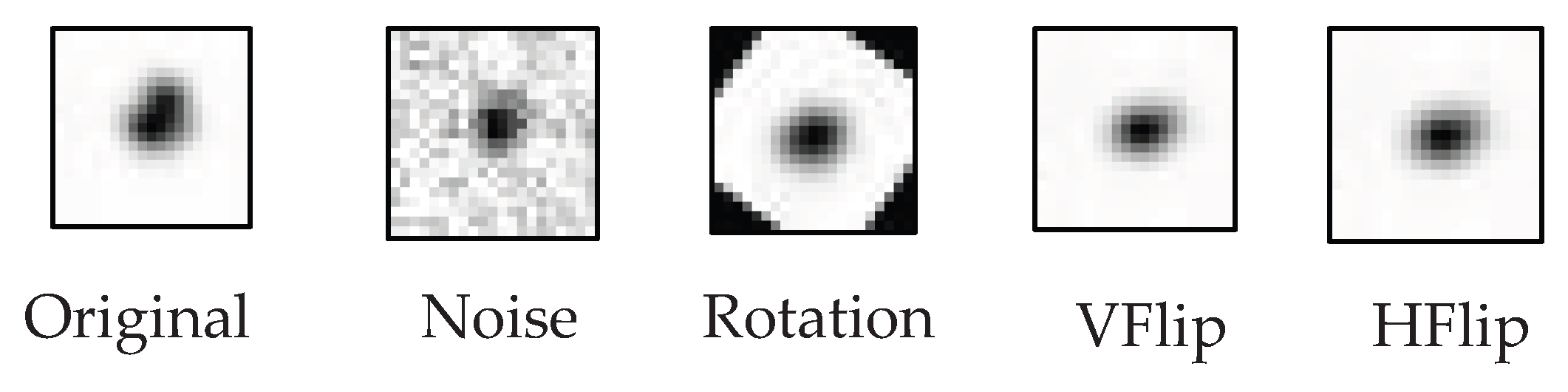
2.3. Data Augmentation
Data augmentation is a well-established technique in deep learning, commonly used to artificially expand the training dataset by applying various transformations to existing images. This process helps improve the generalization capability of the model by exposing it to diverse variations of the data, thereby reducing the risk of overfitting and enhancing final classification accuracy [7].In line with findings from previous studies, we incorporate data augmentation into our training pipeline to increase robustness and improve performance on unseen data. Augmentations such as horizontal flips, rotations, and noise injection are applied to simulate real-world distortions and observational variability. This strategy aims to help the network learn invariant features and become more resilient to subtle differences in transient images.
Figure 3.
An example of data augmentation.
2.4. Modeling
In deep learning for image classification, Convolutional Neural Networks (CNNs) have been widely recognized as powerful tools due to their ability to learn hierarchical representations of spatial features. This capability makes CNNs particularly suitable for image data, especially in the field of astronomy, where precise spatial structure and light distribution are crucial for identifying celestial objects. Over the past decade, a wide range of CNN architectures has been developed, each offering different advantages in terms of network depth, number of parameters, and computational efficiency. In this study, we selected nine CNN architectures to evaluate and compare their performance in classifying astronomical transient images. These architectures include:
- DenseNet121 [8]: Utilizes a dense connectivity mechanism, where each layer receives input from all preceding layers. This promotes feature reuse and alleviates the vanishing gradient problem.
- InceptionV3 [9]: Employs factorized convolutions and efficient dimensionality reduction, enabling deeper networks with lower computational cost.
- MobileNet [10]: Designed for mobile and embedded systems, this architecture uses depthwise separable convolutions to significantly reduce computational complexity.
- MobileNetV2 [11]: An extension of MobileNet, this version introduces inverted residual blocks, enhancing learning capacity while maintaining model compactness.
- ResNet50 and ResNet101 [12]: Implement shortcut connections or identity mappings to combat the vanishing gradient issue and enable effective training of very deep networks.
- VGG16 and VGG19 [13]: Feature a simple and sequential architecture composed of stacked convolutional layers with fixed kernel sizes, known for their consistency and reliability.
- Xception [14]: Evolved from the Inception architecture by replacing all modules with depthwise separable convolutions, offering improved efficiency in extracting fine-grained features.
All nine CNN architectures selected for this study were trained and fine-tuned using consistent hyperparameters as outlined in Table 2. Specifically, we experimented with four different batch sizes (32, 64, 128, and 256) to evaluate their impact on model convergence and generalization. Previous studies have shown that smaller batch sizes (e.g., 32) can lead to better generalization by converging toward flatter minima, while larger batches may reach sharper minima and overfit to training data [15,16]. The number of training epochs was set to a maximum of 100, with Early Stopping applied (patience = 3) to prevent overfitting, a technique widely used in deep learning to halt training once the validation loss no longer improves [17]. For optimization, we employed the Adam optimizer due to its adaptive learning rate, fast convergence, and robustness in noisy gradient settings, which has been demonstrated effective across many neural network architectures [18]. The binary crossentropy loss function was selected, as the classification task involves distinguishing between two classes: real and bogus.
For the transfer learning phase, the initial learning rate was set to 0.001, while during fine-tuning, a significantly smaller learning rate of 0.00001 was used to allow more stable updates in the deeper layers, following best practices that recommend reduced learning rates during fine-tuning to preserve previously learned features and avoid destructive updates [19,20]. In the fine-tuning stage, only the top 30% of convolutional layers were unfrozen and retrained to adapt domain-specific features from astronomical transient images, aligning with guidelines suggesting that selectively unfreezing higher layers is effective, especially when domain shift is moderate and dataset size is limited [21,22] . These hyperparameter settings were uniformly applied across all models to ensure consistency in performance comparisons.

Table 2.
Hyperparameter settings used for training and fine-tuning Convolutional Neural Network (CNN) models for astronomical transient image classification.
Table 2.
Hyperparameter settings used for training and fine-tuning Convolutional Neural Network (CNN) models for astronomical transient image classification.
| Parameter | Value |
|---|---|
| Batch Size | 32,62,128,256 |
| Epoch | 100, Early Stopping (patience = 3) |
| Learning | 0.001(TF), 0.00001(FT) |
| Optimizer | Adam |
| Loss Function | Binary Crossentropy |
| Fine-Tuning unlocks | Top 30% |
2.5. Transfer Learning
Transfer Learning is a process in which knowledge gained from one task (the source task) is transferred to improve learning performance on a different but related task (the target task). In image classification, models pre-trained on large-scale datasets such as ImageNet—with over 14 million images across 1,000 categories—are capable of learning generalized low-level visual features such as edges, contours, and textures. These features can be reused in downstream tasks, particularly when the target dataset is small or domain-specific [23]. In this study, Transfer Learning was implemented using convolutional neural network (CNN) architectures pre-trained on ImageNet. As illustrated in Figure 4, the upper part of the diagram represents the source domain, where the model learns hierarchical features from generic images like cars, trees, and shoes. This knowledge is embedded in the convolutional layers and later transferred to a new domain—astronomical transient image classification [24]. To adapt the model, the original classification head was replaced with a new fully connected classifier specific to the binary classification task of distinguishing between “real” and “bogus” objects. Two training strategies were applied: Transfer Learning, where all convolutional layers are frozen and only the new classifier layers are trained; and Fine-Tuning, where the top 30% of convolutional layers are unfrozen and retrained alongside the classifier to better learn domain-specific patterns [25]. This approach, as shown in Figure 4, enables efficient reuse of prior knowledge while minimizing reliance on large labeled datasets, thus supporting both generalization and domain adaptation in the context of transient astronomical event detection [26].
2.6. Ensemble Deep Learning
In the final phase of this research, Ensemble Learning was employed to further improve classification performance and increase model robustness when dealing with diverse and high-variance image data. As shown in Figure 5, five distinct CNN models were strategically selected to participate in the ensemble. Each model was trained using different Data Augmentation strategies—including Original, Rotation, Horizontal Flip (HFlip), Vertical Flip (VFlip), and Noise Injection—as well as varying Batch Sizes (32, 64, 128, and 256). Architectures such as MobileNet and Xception, under both Transfer Learning (TF) and Fine-Tuning (FT) settings, were chosen based on their prior individual performance on validation datasets. The ensemble system aggregates predictions from these five specialized models through a voting mechanism. This design allows the system to capitalize on the unique strengths of each model—for instance, models trained with rotation-based augmentation are better at recognizing orientation-variant transients, while noise-trained models are more resilient to corrupted or low signal-to-noise data. Studies have demonstrated that such diversity-driven ensemble voting significantly enhances performance and generalization in complex image classification tasks[27,28]. Moreover, voting-based approaches combining augmentation variations (e.g., rotation, flips, preprocessing changes) with CNN ensembles have been shown to outperform single-model setups in medical imaging applications [29]. Ensembles of CNNs leveraging architectural variety and diverse input preprocessing consistently mitigate overfitting and reduce output variance, leading to more robust predictive accuracy [30]. This methodology is particularly effective in astronomical contexts, where transient classification is challenged by variations in image quality, brightness, morphology, and observational conditions. Ensemble Learning thus plays a critical role in ensuring reliable predictions across such complex scenarios.
2.7. Evaluation Methods
Subsequently, the experimental outcomes from each route were gathered and juxtaposed to scrutinize results and efficiency. A comparative analysis of the experimental results from each route was then conducted to assess results and efficacy in the context of scientific classification performance. When evaluating the performance of deep learning models in scientific classification, selecting an appropriate metric is a pivotal factor. Performance indicators such as Recall, Accuracy, and F1-score become crucial in this evaluative process. The precise computational methods for these indicators are delineated in Table 2. Within Table 2, TN represents the count of negative classes accurately predicted as negative, while FP indicates the count of negative classes incorrectly predicted as positive. Conversely, FN illustrates the number of positive classes inaccurately predicted as negative, and TP denotes the number of positive classes accurately predicted as positive. These metrics—particularly Precision, Recall, and F1-score—are widely recommended in binary classification tasks, especially when datasets are imbalanced, because accuracy alone can be misleading (e.g., accuracy paradox) [31]. The F1-score, defined as the harmonic mean of Precision and Recall, provides a balanced measure that penalizes models favoring one at the expense of the other, making it especially valuable when both false positives and false negatives carry significant consequences [32].
Table 2.
Performance indicators and formula.
| Performance indicators | formula |
| Precision (P) | |
| Recall (R) | |
| F1-score | |
| Performance indicators | formula |
| Precision (P) | |
| Recall (R) |
3. Results
3.1. The Classification Performance of Each Model on Each Data Augmentation
In this experiment, the training data consisted entirely of astronomical images augmented using Rotation, with the objective of enhancing the diversity of object orientations and improving the model’s ability to learn from rotationally varied perspectives. A total of nine Convolutional Neural Network (CNN) architectures were tested—DenseNet121, InceptionV3, MobileNet, MobileNetV2, ResNet50, ResNet101, VGG16, VGG19, and Xception—under different batch sizes (32, 64, 128, and 256) and two training strategies: Transfer Learning (TL) and Fine-Tuning (FT).
Table 2.
Comparison of classification results of different deep learning with original dataset.
| Rank | Model | Method | Batch size | Accuracy | F1 Score (bogus) | F1 Score (real) |
| 1 | MobileNet | fine_tuned | 64 | 0.98938 | 0.99393 | 0.95758 |
| 2 | ResNet50 | fine_tuned | 32 | 0.98634 | 0.99222 | 0.94410 |
| 3 | VGG16 | fine_tuned | 32 | 0.98634 | 0.99221 | 0.94479 |
| 4 | VGG19 | fine_tuned | 256 | 0.98331 | 0.99049 | 0.93168 |
| 5 | MobileNet | transfer | 32 | 0.98483 | 0.99130 | 0.94048 |
Table 2.
Comparison of classification results of different deep learning with rotation dataset.
| Rank | Model | Method | Batch size | Accuracy | F1 Score (bogus) | F1 Score (real) |
| 1 | Xception | transfer | 128 | 0.97750 | 0.97739 | 0.97761 |
| 2 | Xception | transfer | 256 | 0.97375 | 0.97352 | 0.97398 |
| 3 | VGG16 | fine_tuned | 128 | 0.97500 | 0.97497 | 0.97503 |
| 4 | VGG19 | fine_tuned | 256 | 0.97188 | 0.97168 | 0.97207 |
| 5 | Xception | fine_tuned | 32 | 0.97188 | 0.97146 | 0.97227 |
The results indicated that Xception consistently outperformed other models, particularly in Transfer Learning at batch size 128, where it achieved an accuracy of 0.97750 and an F1-score (real) of 0.97761, demonstrating exceptional capability in learning rotational patterns. Even in Fine-Tuning with batch size 256, Xception maintained excellent performance, with accuracy of 0.96938 and F1-score (real) of 0.96981, reflecting both high accuracy and stability. Another standout model was VGG16 (Fine-Tuned), which achieved accuracy of 0.97500 and F1-score (real) of 0.97503 at batch size 128, closely matching Xception’s performance and surpassing many other models.
MobileNet, known for its computational efficiency and compact architecture, also performed well in Transfer Learning at batch size 128, with accuracy of 0.96250 and F1-score (real) of 0.96245. However, when fine-tuned, MobileNet displayed signs of overfitting or class imbalance, particularly at batch size 128, where despite a high precision of 0.99826, the recall dropped to 0.71875, resulting in a reduced F1-score of 0.87610. This suggests that additional regularization or balancing techniques may be necessary when applying Rotation to lightweight models like MobileNet.
ResNet50 and ResNet101 exhibited greater variability. For example, ResNet50 fine-tuned at batch size 256 failed completely, with accuracy of 0.5 and F1-score of 0, indicating poor compatibility between deep ResNet architectures and Rotation augmentation without appropriate tuning. On the other hand, ResNet101 fine-tuned at batch size 32 performed well, achieving accuracy of 0.96438 and F1-score (real) of 0.96497, suggesting that smaller batch sizes may be more suitable for deep ResNet models under this augmentation strategy.
MobileNetV2 also demonstrated strong performance, with Transfer Learning at batch size 256 yielding accuracy of 0.96812 and F1-score (real) of 0.96854, which is impressive given the model’s lightweight and energy-efficient design. Similarly, VGG19 showed notable consistency in both Transfer and Fine-Tuned settings, with Fine-Tuned VGG19 at batch size 256 reaching accuracy of 0.97188 and F1-score (real) of 0.97207—among the highest in the experiment.
In conclusion, the results suggest that Xception (Transfer, batch size 128), VGG16 (Fine-Tuned, batch size 128), and VGG19 (Fine-Tuned, batch size 256) were the top three performers under Rotation-based augmentation, maintaining high accuracy and F1-scores across both “bogus” and “real” classes. Meanwhile, models like ResNet50 and MobileNet, in some configurations showed issues with performance imbalance or overfitting, highlighting the need for careful selection, hyperparameter tuning, and possibly the application of additional regularization methods. Ultimately, these findings demonstrate that Rotation alone can be a highly effective augmentation technique, provided that the model architecture and batch size are appropriately matched to the nature of the data.
Table 2.
Comparison of classification results of different deep learning with noise dataset.
| Rank | Model | Method | Batch size | Accuracy | F1 Score (bogus) | F1 Score (real) |
| 1 | Xception | transfer | 128 | 0.97750 | 0.97739 | 0.97761 |
| 2 | Xception | transfer | 256 | 0.97375 | 0.97352 | 0.97398 |
| 3 | VGG16 | fine_tuned | 128 | 0.97500 | 0.97497 | 0.97503 |
| 4 | VGG19 | fine_tuned | 256 | 0.97188 | 0.97168 | 0.97207 |
| 5 | Xception | fine_tuned | 32 | 0.97188 | 0.97146 | 0.97227 |
In this experiment, all models were trained using astronomical image data augmented with Noise, which involves injecting random disturbances into images to simulate the imperfections commonly found in real-world astronomical observations—such as blurring, sensor artifacts, or low-light conditions. The study compared the performance of nine Convolutional Neural Network (CNN) architectures—DenseNet121, InceptionV3, MobileNet, MobileNetV2, ResNet50, ResNet101, VGG16, VGG19, and Xception—under two training strategies: Transfer Learning and Fine-Tuning, across a range of batch sizes (32, 64, 128, and 256).
Overall results indicate that most models failed to effectively learn from noise-augmented data, especially MobileNet, MobileNetV2, VGG16, VGG19, ResNet50, and ResNet101, all of which consistently yielded an accuracy of 0.50000 under all combinations of training strategy and batch size. This strongly suggests a failure in learning or a complete inability to distinguish between classes. Notably, the F1-score for the “real” class was 0.00000, indicating that these models failed to correctly classify any true instances or were severely biased toward the “bogus” (negative) class.
The few models that demonstrated some resilience to the effects of noise were Xception and InceptionV3, which still managed to achieve accuracy and F1-score values above random chance. The Xception model fine-tuned at batch size 256 was the best-performing model in this experiment, achieving an accuracy of 0.72625, precision (bogus) = 0.66667, recall (bogus) = 0.90500, and F1-score (bogus) = 0.76776, with a real-class F1-score of 0.66667—not exceptionally high but significantly better than all other models. Another model with relatively promising results was ResNet50 fine-tuned at batch size 256, which achieved accuracy = 0.85000 and F1-score (real) = 0.83827. While precision and recall were still lower than those observed in non-noise settings, the performance remained reasonably usable.
InceptionV3 showed mixed results, especially under Transfer Learning, where it achieved accuracy of 0.63187 and F1-score (real) = 0.43092 at batch size 32. Although not particularly high, this still indicates some degree of meaningful learning beyond random prediction. However, Fine-Tuning of InceptionV3 across several batch sizes often resulted in F1-scores for the real class dropping below 0.2—or even 0.1—which may indicate overfitting or over-adaptation to the noise, thereby degrading its ability to generalize to true class features.
Interestingly, several models—such as MobileNetV2 (transfer, batch 256)—showed high precision for the “real” class (e.g., 0.75) but extremely low F1-scores (e.g., 0.00746). This disparity suggests that while a few correct predictions may have occurred, the number of predictions for the “real” class was extremely low, leading to very poor recall and severely penalized F1-scores. This reinforces the conclusion that most models failed to cope with noise unless specifically adapted to handle such data.
In summary, the experiment demonstrates that Noise-based Data Augmentation significantly degrades model accuracy across most architectures and training strategies. The most noise-resilient model was Xception (fine-tuned, batch 256), followed by ResNet50 (fine-tuned, batch 256) and InceptionV3 (transfer, batch 32), all of which performed noticeably better than random baselines. However, these findings also underscore the need for advanced techniques—such as denoising preprocessing, noise-aware training strategies, or mixed augmentation pipelines—to enhance model robustness and generalization when training on noisy astronomical data
Table 2.
Comparison of classification results of different deep learning with hflip dataset.
| Rank | Model | Method | Batch size | Accuracy | F1 Score (bogus) | F1 Score (real) |
| 1 | MobileNet | transfer | 64 | 0.99875 | 0.99875 | 0.99875 |
| 2 | Xception | transfer | 32 / 64 | 0.99875 | 0.99875 | 0.99875 |
| 3 | VGG19 | fine_tuned | 32 / 64 | 0.99875 | 0.99875 | 0.99875 |
| 4 | VGG16 | fine_tuned | 64 / 256 | 0.99687 | 0.99688 | 0.99688 |
| 5 | MobileNetV2 | transfer | 256 | 0.99375 | 0.99379 | 0.99379 |
In this experiment, all data were trained using Horizontal Flip (HFlip) as a Data Augmentation technique. This method reflects the images horizontally to increase the diversity of object orientation in astronomical data. The objective was to enhance the capacity of Convolutional Neural Networks (CNNs) to learn object features that may appear flipped when captured by telescopes from different directions. The study involved nine CNN architectures: DenseNet121, InceptionV3, MobileNet, MobileNetV2, ResNet50, ResNet101, VGG16, VGG19, and Xception, evaluated under both Transfer Learning and Fine-Tuning strategies, and across varying Batch Sizes (32, 64, 128, 256).
The results clearly demonstrated that most models performed consistently well, particularly Xception, MobileNet, InceptionV3, VGG16, and VGG19. These models frequently achieved Accuracy near 100% and high F1-scores for both “bogus” and “real” classes. For example, Xception (both transfer and fine-tuned) at batch sizes 64, 128, and 256 achieved Accuracy ranging from 0.99750 to 0.99813, with F1-scores for both classes between 0.99688 and 0.99875. This reflects the model’s deep and precise learning of flipped image characteristics—among the highest-performing results in the experiment.
Similarly, MobileNet (both transfer and fine-tuned) yielded outstanding performance. Notably, MobileNet (transfer, batch 128) achieved Accuracy = 0.99875 and F1-score (real) = 0.99875, comparable to Xception and VGG19 (fine-tuned) under several conditions. InceptionV3 also showed consistently strong results, with transfer models at batch sizes 64, 128, and 256 achieving Accuracy values between 0.99625 and 0.99750, and very high F1-scores across both classes. It is notable that F1-score (real) for these models never dropped below 0.99000 under optimal conditions.
VGG16 and VGG19 also performed remarkably well, especially in fine-tuned mode at batch sizes 64 and 256, achieving Accuracy between 0.99687 and 0.99813, with near-perfect F1-scores in both classes. DenseNet121, particularly in transfer learning mode at batch sizes 128 and 256, consistently produced F1-score (real) > 0.99315, demonstrating the architecture's robustness in learning from horizontally flipped images.
However, some models showed performance degradation. For example, MobileNetV2 (fine-tuned) at batch sizes 32, 64, and 128 exhibited Accuracy between 0.91 and 0.92, with F1-score (real) dropping to approximately 0.91–0.93. Additionally, ResNet101 and ResNet50 under certain conditions—particularly fine-tuned at batch sizes 128 or 256—completely failed to generalize, with Accuracy = 0.50000 and F1-score (real) = 0.00000, indicating an inability to learn or severe overfitting to one class.
In conclusion, Horizontal Flip was found to significantly enhance model performance in learning symmetrical or directionally inverted objects, especially when paired with well-designed deep architectures like Xception, MobileNet, and InceptionV3. While Fine-Tuning generally produced strong results, Transfer Learning also proved capable of generating powerful models—offering an efficient training strategy under limited computational resources. Therefore, HFlip can be considered a highly effective augmentation technique for improving classification accuracy in astronomical image analysis.
Table 2.
Comparison of classification results of different deep learning with vflip dataset.
| Rank | Model | Method | Batch size | Accuracy | F1 Score (bogus) | F1 Score (real) |
| 1 | MobileNet | transfer | 64 | 0.99875 | 0.99875 | 0.99875 |
| 2 | Xception | transfer | 32 / 64 | 0.99875 | 0.99875 | 0.99875 |
| 3 | VGG19 | fine_tuned | 32 / 64 | 0.99875 | 0.99875 | 0.99875 |
| 4 | VGG16 | fine_tuned | 64 / 256 | 0.99687 | 0.99688 | 0.99688 |
| 5 | MobileNetV2 | transfer | 256 | 0.99375 | 0.99379 | 0.99379 |
In this experiment, the dataset was augmented using Vertical Flip (VFlip)—a technique that mirrors astronomical images along the vertical axis—to enhance the model's ability to learn features from objects captured in reversed vertical orientations. This method is particularly valuable in astronomical image analysis, where object positions and orientations can vary across different observations. The experiment involved nine CNN architectures—DenseNet121, InceptionV3, MobileNet, MobileNetV2, ResNet50, ResNet101, VGG16, VGG19, and Xception—under both Transfer Learning and Fine-Tuning strategies, and across various Batch Sizes (32, 64, 128, and 256). The overall results demonstrated that deeper and structurally efficient models effectively handled the vertical flipping transformation. Specifically, models such as MobileNet, Xception, InceptionV3, VGG19, and VGG16 achieved consistently high performance across all key evaluation metrics—Accuracy, Precision, Recall, and F1-score—for both “bogus” and “real” classes. Notably, MobileNet (transfer) and VGG19 (fine-tuned) at batch sizes of 32, 64, and 128 achieved Accuracy and F1-score as high as 0.99875, indicating near-perfect classification of vertically flipped images.
Similarly, Xception (transfer) at batch size 256 reached Accuracy = 0.99813 and identical F1-scores of 0.99813 for both classes. Xception consistently maintained high performance across all batch sizes and training strategies. However, in some cases, such as Xception fine-tuned at batch 256, Accuracy slightly decreased to 0.98000 and F1-score (real) = 0.98039, which remains remarkably high and commendable.
Other models like DenseNet121 also showed excellent results, with transfer learning at batch sizes 32 or 64 yielding Accuracy between 0.99125 and 0.99313 and F1-score (real) exceeding 0.991. Similarly, InceptionV3 (transfer) at batch sizes 64 and 128 achieved Accuracy up to 0.99687 and F1-score (real) > 0.99688, reflecting robust and consistent performance. Despite their older architecture, VGG16 and VGG19 maintained outstanding accuracy—VGG16 fine-tuned at batch 256 achieved Accuracy = 0.99687 and F1-score (real) = 0.99688, comparable to top-performing models like Xception and MobileNet.
In contrast, models such as ResNet50 and ResNet101 exhibited more volatile performance. Specifically, ResNet101 fine-tuned at batch sizes 128 and 256 showed Accuracy = 0.50000 and F1-score (real) = 0.00000, indicating potential overfitting or heightened sensitivity to vertical flipping transformations. However, ResNet101 (transfer) at batch sizes 64 and 256 still produced Accuracy values around 0.92–0.93 and F1-score (real) > 0.92, suggesting that transfer learning may help mitigate VFlip's impact on ResNet's performance.
In summary, the experiment clearly shows that Vertical Flip (VFlip) augmentation significantly enhances model performance when applied with the right architectures particularly Xception, MobileNet, InceptionV3, VGG19, and VGG16. Fine-Tuning with moderate batch sizes (e.g., 64 or 128) consistently yielded very high evaluation scores. Moreover, Transfer Learning proved sufficient for models like MobileNet and Xception, achieving high performance without full retraining. Thus, VFlip stands out as a highly effective augmentation technique, especially in real-world systems requiring robustness and accuracy in scenarios with unpredictable image orientation.
3.2. The Classification Performance of Ensemble Deep Learning
In the previous section, various Convolutional Neural Network (CNN) architectures were trained and evaluated under different conditions using techniques such as Data Augmentation and parameter tuning, including the application of Transfer Learning and Fine-Tuning, alongside adjustments to the Batch Size. These experiments aimed to investigate how different training strategies affect the model's ability to classify astronomical images in complex and uncertain scenarios. Preliminary results revealed that several models—particularly Xception, MobileNet, InceptionV3, VGG16, and VGG19—consistently maintained strong performance across a range of augmented datasets, including Original, Vertical Flip, Horizontal Flip, and Rotation. These models sustained high levels of Accuracy, Precision, Recall, and F1-score across most experimental settings under both Transfer Learning and Fine-Tuning approaches. This demonstrates the flexibility and structural robustness of these architectures in handling spatial transformations and symmetrical variations commonly found in astronomical image data. However, a significant limitation that warrants special attention for future development is the models' vulnerability to noise-augmented data. Noise augmentation was used to simulate real-world imperfections in astronomical imagery, such as sensor interference or unfavorable environmental conditions. Under these conditions, most models showed a noticeable drop in performance, with Accuracy and F1-score falling below usable thresholds in many cases—especially in the “real” class, where some models recorded an F1-score of 0.00000, indicating a complete failure to identify true astronomical objects. These results highlight the presence of bias and a lack of generalization capability when dealing with high levels of noise.
The models with the best performance for each type of data transformation (as identified in the previous experimental sections) were selected based on both Accuracy and F1-score, considering the most effective Batch Size for each case, as follows:
Table 2.
Selected Models for Ensemble Based on Best Performance by Augmentation Type.
| Model | Method | Augmentation | Batch Size |
| MobileNet | Fine-Tuned | Original | 64 |
| Xception | Transfer | Rotation | 128 |
| Xception | Fine-Tuned | Noise | 256 |
| MobileNet | Transfer | HFlip | 64 |
| MobileNet | Transfer | VFlip | 32 |
3.1.1. Experimental Results of Model Combination Using Soft Voting Ensemble Technique
The experimental results using the Soft Voting Ensemble technique, which combined multiple models trained with various data augmentation strategies, demonstrated a promising level of performance in astronomical image classification. The ensemble model achieved strong results in the “bogus” class, with a precision of 0.7513, a remarkably high recall of 0.9957, and an F1-score of 0.8564. However, in the “real” class, while precision remained very high at 0.9922, the recall dropped significantly to 0.62143, resulting in an F1-score of 0.764. This indicates that the model performed well in identifying negative instances but struggled to detect true astronomical objects accurately. The overall accuracy of the ensemble was 0.8215, reflecting moderate general performance across mixed data conditions. The confusion matrix further supports these observations: the model correctly identified 4,696 bogus instances out of 4,716, while it misclassified 1,554 real instances as bogus out of a total of 4,105 real samples. This substantial number of false negatives in the real class explains the low recall and highlights a critical limitation in the ensemble’s generalization when encountering real, often more complex, image structures. When evaluating performance by augmentation type, both HFlip and VFlip produced excellent results, with HFlip achieving a precision of 0.995, recall of 0.986, and an F1-score of 0.9905—demonstrating the model’s ability to learn symmetrical spatial features effectively. Rotation-based augmentation also performed relatively well, with an F1-score of 0.6936, although its slightly lower recall suggests challenges in recognizing rotated features. The original dataset without augmentation yielded a high F1-score of 0.972, indicating the model's strong capacity to classify undistorted data. However, the model performed poorly on noise-augmented data, where the F1-score plummeted to 0.002, driven by an extremely low recall of 0.001. This suggests a nearly complete inability to detect real objects in the presence of signal distortion, underscoring the model’s vulnerability to noisy environments. In conclusion, the Soft Voting ensemble strategy enhances classification accuracy in scenarios involving symmetrical or geometrically transformed images. Nonetheless, the model’s performance deteriorates under high-noise conditions, indicating a need for further improvements. Future work may consider employing Weighted Voting strategies that give greater influence to noise-trained models or implementing preprocessing techniques to reduce noise before model training. Such enhancements could significantly improve model robustness and applicability in real-world astronomical imaging, where imperfect and noisy data are often unavoidable.
Table 2.
Test with data.
| Model | Accuracy | Precision (bogus) | Recall (bogus) | F1 Score (bogus) | Precision (real) | Recall (real) | F1 Score (real) |
| Ensemble | 0.8215 | 0.7513 | 0.9957 | 0.8564 | 0.9922 | 0.62143 | 0.764 |
Confusion Matrix
| Pred: bogus | Pred: real | |
| True: bogus | 4696 | 20 |
| True: real | 1554 | 2551 |
Table 2.
Experimental Results of Model Combination Using Soft Voting Ensemble Technique pre data augmentation.
Table 2.
Experimental Results of Model Combination Using Soft Voting Ensemble Technique pre data augmentation.
| Augmentation | TP | TN | FP | FN | Precision | Recall | F1-Score |
| HFlip | 986 | 995 | 5 | 14 | 0.995 | 0.986 | 0.9905 |
| Noise | 1 | 1000 | 0 | 999 | 1 | 0.001 | 0.002 |
| Rotation | 473 | 994 | 6 | 527 | 0.9875 | 0.473 | 0.6396 |
| VFlip | 987 | 996 | 4 | 13 | 0.996 | 0.987 | 0.9915 |
| original | 104 | 711 | 5 | 1 | 0.9541 | 0.9905 | 0.972 |
3.1.1. Experimental Results of Model Combination Using Weighted Voting Ensemble Technique
From the experiments comparing Soft Voting and Weighted Voting techniques, it was observed that Soft Voting yielded the lowest overall accuracy, and the issue of Noise remained a major challenge in astronomical image classification. To address this, the strategy was shifted to Weighted Voting, where model weights were adjusted based on their training configurations. In particular, greater emphasis was placed on the model trained with Noise-augmented data in an attempt to improve the system’s resilience to signal distortions. In the first Weighted Voting experiment, the weight assigned to the Noise-based model was set at 0.3. However, the results indicated that this adjustment was insufficient, as the accuracy remained low and the confusion matrix revealed a high rate of misclassification, especially in the real class. Subsequently, the weight for the Noise-trained model was increased to 0.5 in the second experiment. The performance showed notable improvement, especially in handling noisy data, suggesting a positive trend whereby increasing the weight of the Noise model could enhance overall robustness. Building upon this trend, the third experiment assigned a weight of 0.8 to the Noise model, resulting in the best performance across all tests. The ensemble achieved an overall accuracy of 0.972, significantly outperforming previous configurations. These results highlight the importance of strategic weight allocation in Weighted Voting ensembles and demonstrate that increasing the influence of models trained to handle challenging conditions—such as Noise—can substantially improve classification performance in complex and imperfect data environments.
Table 2.
Parameter in first ensemble.
| Model | Method | Batch Size | Augmentation | Weight |
| MobileNet | fine_tuned | 64 | Original | 0.2 |
| Xception | transfer | 128 | Rotation | 0.2 |
| Xception | fine_tuned | 256 | Noise | 0.3 |
| MobileNet | transfer | 64 | HFlip | 0.15 |
| MobileNet | Transfer | 32 | VFlip | 0.15 |
Table 2.
Test with data.
| Model | Accuracy | Precision (bogus) | Recall (bogus) | F1 Score (bogus) | Precision (real) | Recall (real) | F1 Score (real) |
| Ensemble | 0.8204 | 0.7512 | 0.993 | 0.855 | 0.987 | 0.6221 | 0.763 |
Confusion Matrix
| Pred: bogus | Pred: real | |
| True: bogus | 4683 | 33 |
| True: real | 1551 | 2554 |
Table 2.
Experimental Results of Model Combination Using Weighted Voting Ensemble Technique pre data augmentation.
Table 2.
Experimental Results of Model Combination Using Weighted Voting Ensemble Technique pre data augmentation.
| Augmentation | TP | TN | FP | FN | Precision | Recall | F1-Score |
| HFlip | 966 | 990 | 10 | 34 | 0.9898 | 0.966 | 0.9777 |
| Noise | 5 | 1000 | 0 | 995 | 1 | 0.001 | 0.0100 |
| Rotation | 509 | 992 | 8 | 491 | 0.9845 | 0.509 | 0.6711 |
| VFlip | 969 | 991 | 9 | 31 | 0.9908 | 0.969 | 0.9798 |
| original | 105 | 710 | 6 | 0 | 0.9459 | 1.00 | 0.9722 |
Table 2.
Parameter in second ensemble.
| Model | Method | Batch Size | Augmentation | Weight |
| MobileNet | fine_tuned | 64 | Original | 0.2 |
| Xception | transfer | 128 | Rotation | 0.2 |
| Xception | fine_tuned | 256 | Noise | 0.50 |
| MobileNet | transfer | 64 | HFlip | 0.15 |
| MobileNet | Transfer | 32 | VFlip | 0.15 |
Table 2.
Test with data.
| Model | Accuracy | Precision (bogus) | Recall (bogus) | F1 Score (bogus) | Precision (real) | Recall (real) | F1 Score (real) |
| Ensemble | 0.8852 | 0.830 | 0.9866 | 0.901 | 0.980 | 0.7688 | 0.861 |
Confusion Matrix
| Pred: bogus | Pred: real | |
| True: bogus | 4653 | 63 |
| True: real | 949 | 3156 |
Table 2.
Experimental Results of Model Combination Using Weighted Voting Ensemble Technique pre data augmentation.
Table 2.
Experimental Results of Model Combination Using Weighted Voting Ensemble Technique pre data augmentation.
| Augmentation | TP | TN | FP | FN | Precision | Recall | F1-Score |
| HFlip | 962 | 962 | 13 | 38 | 0.9867 | 0.962 | 0.9742 |
| Noise | 277 | 985 | 15 | 723 | 0.9486 | 0.277 | 0.4288 |
| Rotation | 845 | 986 | 14 | 155 | 0.9837 | 0.845 | 0.9097 |
| VFlip | 967 | 987 | 13 | 33 | 0.9867 | 0.967 | 0.9768 |
| original | 105 | 708 | 8 | 0 | 0.9292 | 1.00 | 0.9633 |
Table 2.
Parameter in third ensemble.
| Model | Method | Batch Size | Augmentation | Weight |
| MobileNet | fine_tuned | 64 | Original | 0.20 |
| Xception | transfer | 128 | Rotation | 0.20 |
| Xception | fine_tuned | 256 | Noise | 0.80 |
| MobileNet | transfer | 64 | HFlip | 0.15 |
| MobileNet | Transfer | 32 | VFlip | 0.15 |
Table 2.
Test with data.
| Model | Accuracy | Precision (bogus) | Recall (bogus) | F1 Score (bogus) | Precision (real) | Recall (real) | F1 Score (real) |
| Ensemble | 0.9348 | 0.951 | 0.925 | 0.938 | 0.916 | 0.945 | 0.931 |
Confusion Matrix
| Pred: bogus | Pred: real | |
| True: bogus | 4364 | 352 |
| True: real | 223 | 3882 |
Table 2.
Experimental Results of Model Combination Using Weighted Voting Ensemble Technique pre data augmentation.
Table 2.
Experimental Results of Model Combination Using Weighted Voting Ensemble Technique pre data augmentation.
| Augmentation | TP | TN | FP | FN | Precision | Recall | F1-Score |
| HFlip | 959 | 968 | 32 | 41 | 0.9677 | 0.959 | 0.9633 |
| Noise | 1000 | 772 | 228 | 0 | 0.8143 | 1.00 | 0.8977 |
| Rotation | 855 | 950 | 50 | 145 | 0.9448 | 0.855 | 0.8976 |
| VFlip | 967 | 970 | 30 | 36 | 0.9698 | 0.9640 | 0.9669 |
| original | 104 | 704 | 12 | 1 | 0.8966 | 0.9905 | 0.9412 |
4. Discussion
The experimental results clearly demonstrate the effectiveness of integrating advanced Convolutional Neural Network (CNN) architectures with strategic Data Augmentation, Transfer Learning, Fine-Tuning, and Ensemble Learning in the context of astronomical transient detection. Several critical insights can be drawn from these findings.
4.1. Performance of Individual CNN Models
Across all augmentation strategies, models such as Xception, MobileNet, and VGG16/19 consistently outperformed others in both accuracy and F1-score. In particular, Xception with Transfer Learning and batch size 128 achieved the highest performance on rotation-augmented data, while MobileNet (Fine-Tuned) performed exceptionally on the original dataset. These results emphasize the flexibility and structural robustness of certain architectures in learning domain-specific patterns, especially those involving spatial symmetry, orientation variations, and brightness inconsistencies commonly observed in transient astronomical imagery.
However, not all architectures responded equally well to each augmentation technique. For instance, ResNet50 and ResNet101 displayed significant performance degradation under some configurations—most notably with noise-augmented data and larger batch sizes. This suggests that deeper architectures may require more sophisticated regularization or denoising techniques when handling corrupted or low-SNR images.
4.2. Impact of Data Augmentation
Among the augmentation strategies tested, Horizontal Flip (HFlip) and Vertical Flip (VFlip) yielded the most consistently high classification performance across all models, often resulting in F1-scores above 0.99. This indicates that these transformations effectively simulate the positional variability of transient objects and assist CNNs in learning rotational-invariant features.
In contrast, Noise augmentation proved to be the most challenging for nearly all models. Most architectures failed completely under noisy conditions, yielding F1-scores as low as 0.000, indicating severe overfitting or class bias. Only a few models, notably Xception and ResNet50, managed to retain marginal classification ability. This highlights a key vulnerability in current deep learning models applied to astronomical imagery: their sensitivity to image noise, which is a prevalent issue in real observational data.
These findings emphasize the need for future research to focus on improving robustness against noise—either through preprocessing (e.g., denoising filters), adversarial training, or noise-aware model architectures.
4.3. Effectiveness of Ensemble Learning
To address the weaknesses of individual models—particularly under noise-augmented conditions—this study explored Soft Voting and Weighted Voting ensemble strategies. The Soft Voting ensemble offered moderate improvements in accuracy but remained limited by its uniform weighting scheme, which failed to sufficiently correct performance imbalance under noisy conditions. Specifically, recall in the “real” class was consistently low, indicating a failure to detect true transient events reliably.
In contrast, Weighted Voting allowed more flexibility by assigning higher influence to noise-trained models. A progressive tuning of weights in three ensemble configurations demonstrated that increasing the weight of the noise-robust model (up to 0.8) significantly improved overall performance, culminating in an F1-score (real) of 0.931 and an overall accuracy of 0.9348. This supports the hypothesis that ensemble strategies which explicitly compensate for weak conditions—such as noise corruption—can substantially improve model generalization and classification balance.
Notably, the final ensemble configuration not only corrected recall degradation but also maintained strong performance across other augmentation types, demonstrating its adaptability and robustness in complex, heterogeneous astronomical datasets.
4.4. Generalization and Scalability
The success of this ensemble approach illustrates the potential of combining multiple specialized models to form a unified system capable of handling the high variance and complexity of real-world astronomical data. The pipeline’s design—featuring modular training, augmentation-specific modeling, and intelligent voting—offers a scalable solution that can be extended to other sky surveys and transient detection projects. Furthermore, the system’s reliance on Transfer Learning and moderate fine-tuning suggests that this approach is computationally efficient and suitable for deployment in time-critical applications, such as real-time transient detection in large-scale surveys like GOTO.
5. Conclusions
This study introduced an ensemble-based deep learning framework designed to classify real and bogus astronomical transients from sky survey images. By integrating Transfer Learning, Fine-Tuning, multiple Data Augmentation strategies (such as Rotation, Horizontal Flip, Vertical Flip, and Noise), and Ensemble Learning techniques, the proposed system achieved substantial improvements in classification accuracy and robustness. Models like Xception, MobileNet, and VGG19 consistently outperformed others, particularly under augmentation strategies that introduced geometric variations. While most models struggled with noise-injected images, the Weighted Voting strategy—especially when assigning higher weights to noise-trained models—greatly enhanced the system’s resilience to distortion and improved the F1-score of the “real” class to 0.931 with an overall accuracy of 93.48%. These results highlight the importance of model diversity and strategic ensemble configuration for addressing the challenges of real-world astronomical datasets. The proposed approach offers a scalable and practical solution for transient detection tasks in large-scale sky surveys and lays the groundwork for future research in noise-resilient deep learning for astronomy.
References
- B. P. Abbott et al., “GW170817: Observation of Gravitational Waves from a Binary Neutron Star Inspiral,” Phys. Rev. Lett., vol. 119, no. 16, p. 161101, Oct. 2017. [CrossRef]
- B. D. Metzger, “Kilonovae,” Living Rev. Relativ., vol. 23, no. 1, p. 1, 2020.
- H. Domínguez Sánchez, M. Huertas-Company, M. Bernardi, D. Tuccillo, and J. L. Fischer, “Improving galaxy morphologies for SDSS with Deep Learning,” Mon. Not. R. Astron. Soc., vol. 476, no. 3, pp. 3661–3676, 2018. [CrossRef]
- G. Cabrera-Vives, I. Reyes, F. Förster, P. A. Estévez, and J.-C. Maureira, “Deep-HiTS: Rotation Invariant Convolutional Neural Network for Transient Detection∗,” Astrophys. J., vol. 836, no. 1, p. 97, 2017. [CrossRef]
- N. Srivastava, G. Hinton, A. Krizhevsky, I. Sutskever, and R. Salakhutdinov, “Dropout: a simple way to prevent neural networks from overfitting,” J. Mach. Learn. Res., vol. 15, no. 1, pp. 1929–1958, 2014.
- Priyadarshini and V. Puri, “A convolutional neural network (CNN) based ensemble model for exoplanet detection,” Earth Sci. Inform., vol. 14, no. 2, pp. 735–747, June 2021. [CrossRef]
- G. García-Jara, P. Protopapas, and P. A. Estévez, “Improving astronomical time-series classification via data augmentation with generative adversarial networks,” Astrophys. J., vol. 935, no. 1, p. 23, 2022. [CrossRef]
- G. Huang, Z. Liu, L. Van Der Maaten, and K. Q. Weinberger, “Densely connected convolutional networks,” in Proceedings of the IEEE conference on computer vision and pattern recognition, 2017, pp. 4700–4708.
- C. Szegedy, V. Vanhoucke, S. Ioffe, J. Shlens, and Z. Wojna, “Rethinking the inception architecture for computer vision,” in Proceedings of the IEEE conference on computer vision and pattern recognition, 2016, pp. 2818–2826.
- A. G. Howard et al., “Mobilenets: Efficient convolutional neural networks for mobile vision applications,” ArXiv Prepr. ArXiv170404861, 2017.
- M. Sandler, A. Howard, M. Zhu, A. Zhmoginov, and L.-C. Chen, “Mobilenetv2: Inverted residuals and linear bottlenecks,” in Proceedings of the IEEE conference on computer vision and pattern recognition, 2018, pp. 4510–4520. [CrossRef]
- K. He, X. Zhang, S. Ren, and J. Sun, “Deep residual learning for image recognition,” in Proceedings of the IEEE conference on computer vision and pattern recognition, 2016, pp. 770–778.
- K. Simonyan and A. Zisserman, “Very deep convolutional networks for large-scale image recognition,” ArXiv Prepr. ArXiv14091556, 2014.
- F. Chollet, “Xception: Deep learning with depthwise separable convolutions,” in Proceedings of the IEEE conference on computer vision and pattern recognition, 2017, pp. 1251–1258.
- D. Masters and C. Luschi, “Revisiting small batch training for deep neural networks,” ArXiv Prepr. ArXiv180407612, 2018.
- N. S. Keskar, D. Mudigere, J. Nocedal, M. Smelyanskiy, and P. T. P. Tang, “On large-batch training for deep learning: Generalization gap and sharp minima,” ArXiv Prepr. ArXiv160904836, 2016.
- L. Prechelt, “Early stopping-but when?,” in Neural Networks: Tricks of the trade, Springer, 2002, pp. 55–69.
- D. Kinga and J. B. Adam, “A method for stochastic optimization,” in International conference on learning representations (ICLR), San Diego, California;, 2015.
- M. Iman, H. R. Arabnia, and K. Rasheed, “A review of deep transfer learning and recent advancements,” Technologies, vol. 11, no. 2, p. 40, 2023. [CrossRef]
- N. Becherer, J. Pecarina, S. Nykl, and K. Hopkinson, “Improving optimization of convolutional neural networks through parameter fine-tuning,” Neural Comput. Appl., vol. 31, pp. 3469–3479, 2019. [CrossRef]
- Kandel and M. Castelli, “How deeply to fine-tune a convolutional neural network: a case study using a histopathology dataset,” Appl. Sci., vol. 10, no. 10, p. 3359, 2020. [CrossRef]
- X. Xiao, T. B. Mudiyanselage, C. Ji, J. Hu, and Y. Pan, “Fast deep learning training through intelligently freezing layers,” in 2019 international conference on internet of things (iThings) and IEEE green computing and communications (GreenCom) and IEEE cyber, physical and social computing (CPSCom) and IEEE smart data (SmartData), IEEE, 2019, pp. 1225–1232. [CrossRef]
- Q. Yang, “An Introduction to Transfer Learning.,” in ADMA, Springer, 2008, p. 1.
- G. Vrbančič and V. Podgorelec, “Transfer learning with adaptive fine-tuning,” IEEE Access, vol. 8, pp. 196197–196211, 2020. [CrossRef]
- T. Shermin, S. W. Teng, M. Murshed, G. Lu, F. Sohel, and M. Paul, “Enhanced transfer learning with imagenet trained classification layer,” in Image and Video Technology: 9th Pacific-Rim Symposium, PSIVT 2019, Sydney, NSW, Australia, November 18–22, 2019, Proceedings 9, Springer, 2019, pp. 142–155. 18 November.
- Y. Cui, Y. Song, C. Sun, A. Howard, and S. Belongie, “Large scale fine-grained categorization and domain-specific transfer learning,” in Proceedings of the IEEE conference on computer vision and pattern recognition, 2018, pp. 4109–4118.
- M. A. Ganaie, M. Hu, A. K. Malik, M. Tanveer, and P. N. Suganthan, “Ensemble deep learning: A review,” Eng. Appl. Artif. Intell., vol. 115, p. 105151, 2022.
- U. Muñoz-Aseguinolaza, B. Sierra, and N. Aginako, “Rotational augmentation techniques: a new perspective on ensemble learning for image classification,” ArXiv Prepr. ArXiv230607027, 2023.
- E. Tasci, C. Uluturk, and A. Ugur, “A voting-based ensemble deep learning method focusing on image augmentation and preprocessing variations for tuberculosis detection,” Neural Comput. Appl., vol. 33, no. 22, pp. 15541–15555, 2021. [CrossRef]
- T. Shibata, M. Tanaka, and M. Okutomi, “Geometric Data Augmentation Based On Feature Map Ensemble,” in 2021 IEEE International Conference on Image Processing (ICIP), IEEE, 2021, pp. 904–908.
- O. Rainio, J. Teuho, and R. Klén, “Evaluation metrics and statistical tests for machine learning,” Sci. Rep., vol. 14, no. 1, p. 6086, 2024. [CrossRef]
- T. Saito and M. Rehmsmeier, “The precision-recall plot is more informative than the ROC plot when evaluating binary classifiers on imbalanced datasets,” PloS One, vol. 10, no. 3, p. e0118432, 2015. [CrossRef]
Figure 1.
This is a figure. Show the overall methods.
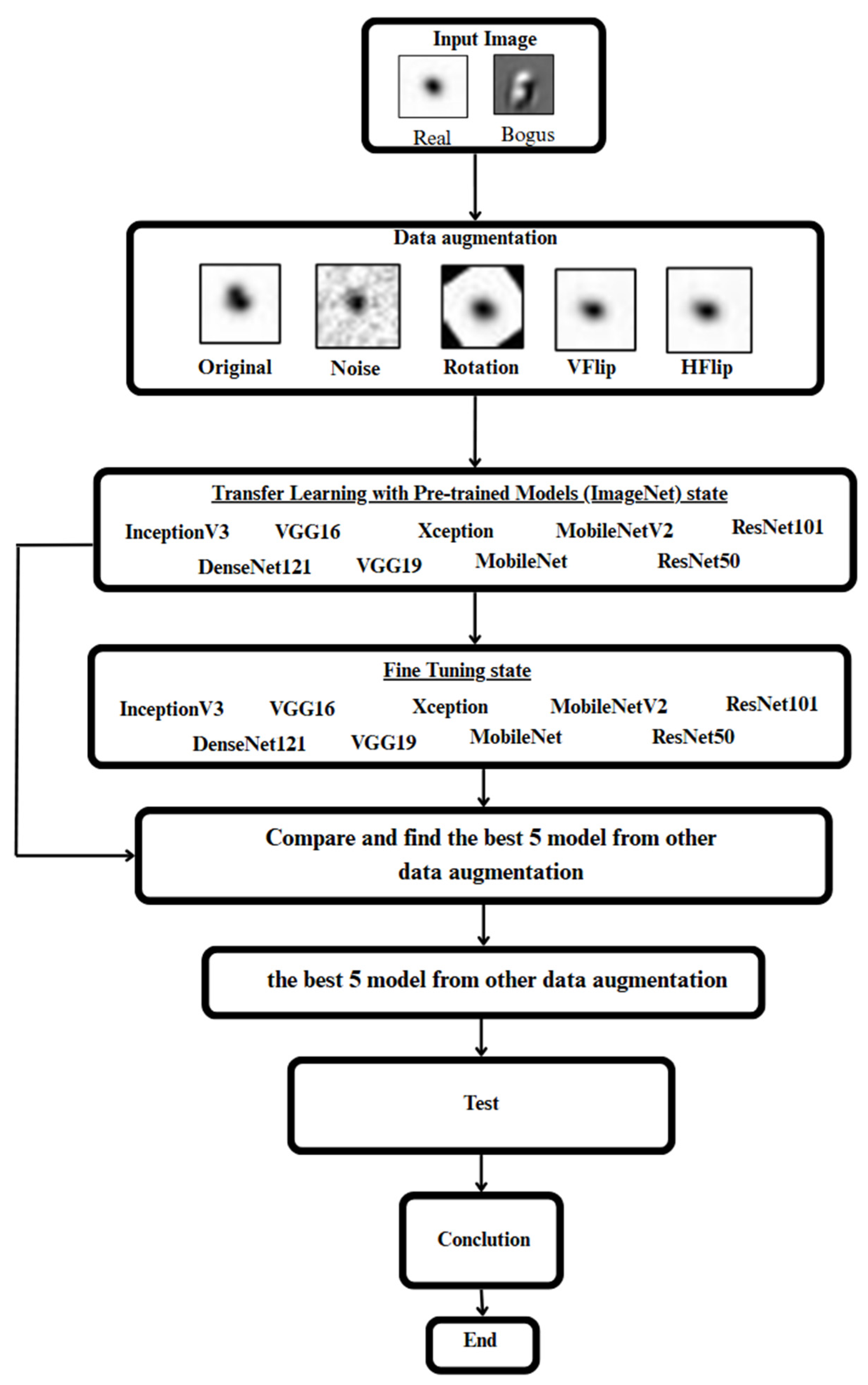
Figure 2.
This is a figure. Show the overall methods
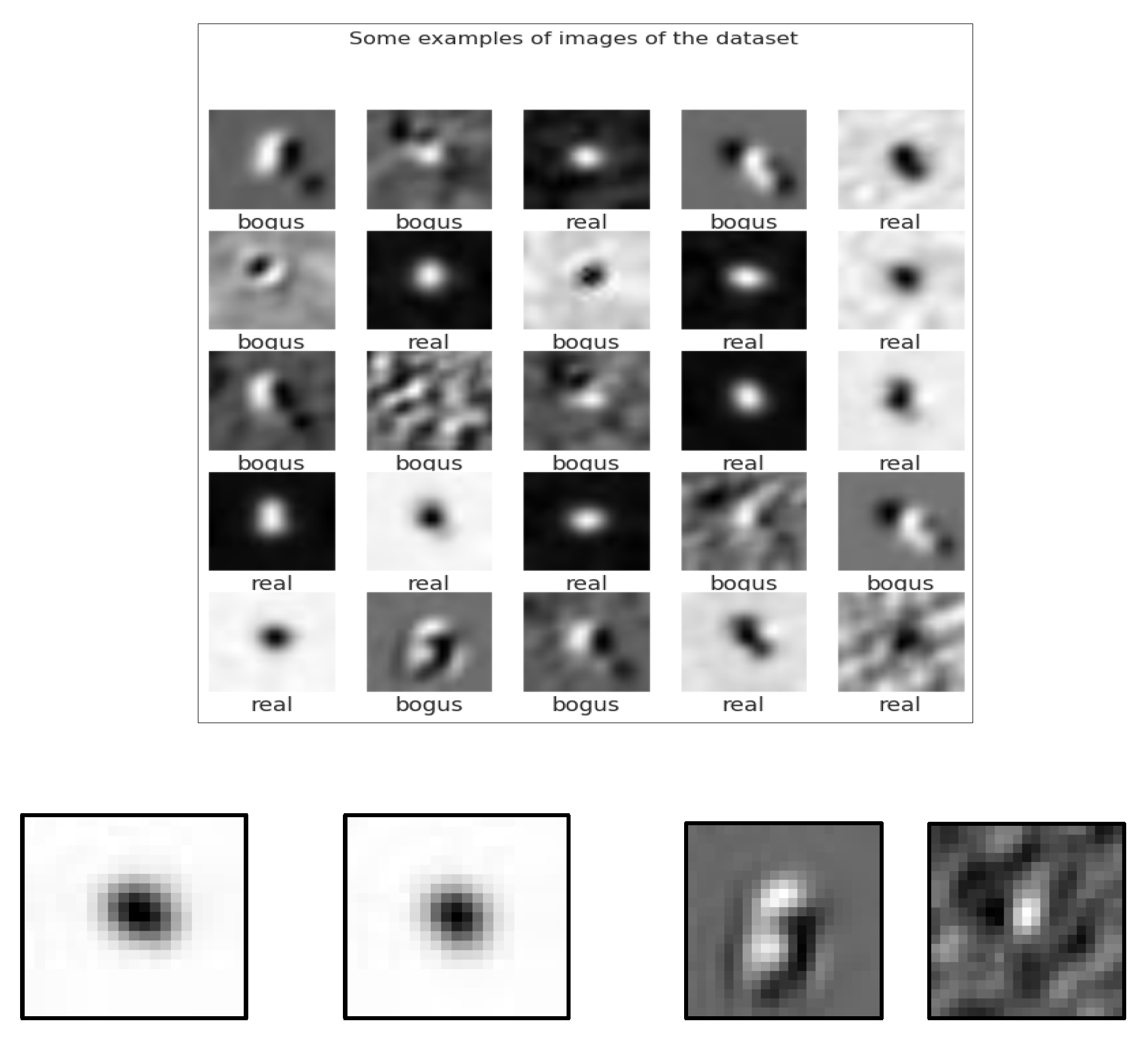
Figure 4.
The process of transferring learned features from a source domain (ImageNet) to a target domain (astronomical transient data) using the Transfer Learning approach.
Figure 4.
The process of transferring learned features from a source domain (ImageNet) to a target domain (astronomical transient data) using the Transfer Learning approach.
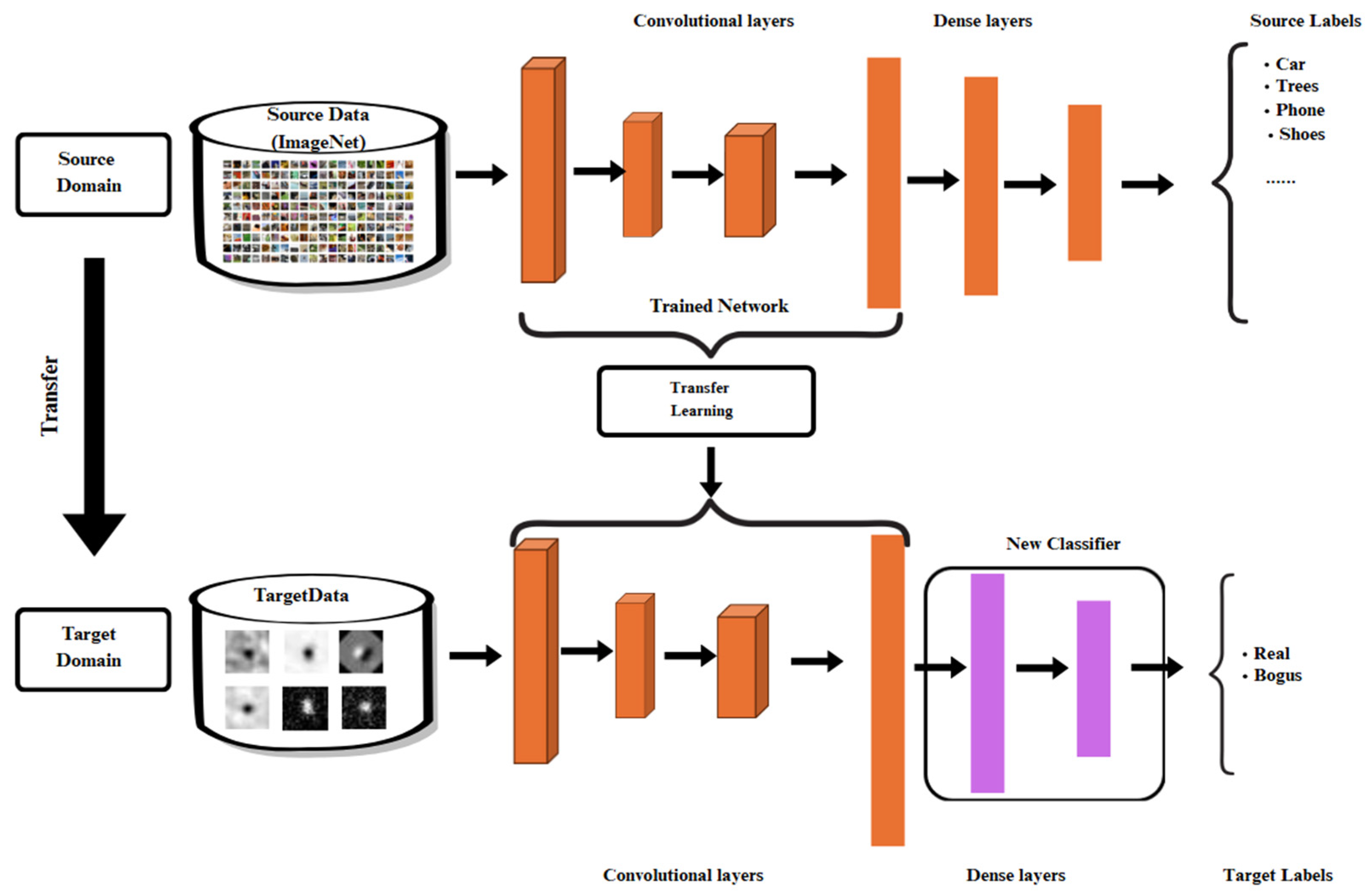
Figure 5.
Ensemble architecture combining multiple CNN models trained under different augmentation strategies and batch sizes.
Figure 5.
Ensemble architecture combining multiple CNN models trained under different augmentation strategies and batch sizes.
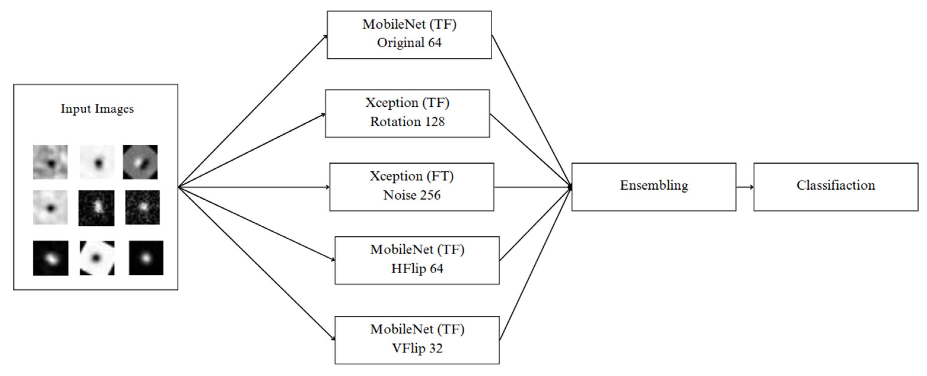
Table 1.
Training data before and after oversampling.
| Training data | Bogus | Real |
| Before Oversampling | 2,862 | 418 |
| After Oversampling | 4,000 | 4,000 |
Disclaimer/Publisher’s Note: The statements, opinions and data contained in all publications are solely those of the individual author(s) and contributor(s) and not of MDPI and/or the editor(s). MDPI and/or the editor(s) disclaim responsibility for any injury to people or property resulting from any ideas, methods, instructions or products referred to in the content. |
© 2025 by the authors. Licensee MDPI, Basel, Switzerland. This article is an open access article distributed under the terms and conditions of the Creative Commons Attribution (CC BY) license (https://creativecommons.org/licenses/by/4.0/).
Copyright: This open access article is published under a Creative Commons CC BY 4.0 license, which permit the free download, distribution, and reuse, provided that the author and preprint are cited in any reuse.


