Submitted:
30 August 2025
Posted:
01 September 2025
You are already at the latest version
Abstract
A maneuver model for a duct-jet propelled autonomous underwater vehicle is developed based on unsteady Reynolds averaged Navier–Stokes solutions. The target meter-class vehicle is cylindrical equipped with four cross-type rudders and a ducted propeller operating at a Froude number of 0.39. A conventional propulsion modelling approach based on propeller open water characteristics is employed to embed the duct-jet propulsive model, while axial flow speeds near the duct inlet are additionally extracted from both propeller open-water and static-drift tests. For practical implementation, the number of captive simulations required to extract maneuvering coefficients is reduced, with the kinematic model compensating for the limited dataset. Validation against the high-fidelity simulation indicates that the surrogate model effectively reproduces free-running results for kinematic variables, forces and moment by manifesting dominant features. For the evaluation of solution sensitivity due to spatial discretization, verification studies employing a grid triplet are focused on hull body resistance and propulsion characteristics.
Keywords:
hydrodynamics
; computational fluid dynamics
; star-ccm
; surrogate
; autonomous underwater vehicle
; duct-jet
; propeller open water test
; planar motion mechanism
1. Introduction
Autonomous Underwater Vehicles (AUVs) have emerged as one of the most actively studied technologies in marine engineering, driven by their versatility across scientific, industrial, and defense applications. Unlike traditional manned or remotely operated systems, AUVs offer persistent and cost-effective operation in hazardous and remote environments, reducing risks to human operators while expanding the scope of underwater exploration. Their capability to operate independently makes them particularly attractive for missions such as seabed mapping, environmental monitoring, infrastructure inspection, and naval reconnaissance [1,2,3].
Recent years have witnessed rapid advancements in the enabling technologies that underpin AUV design and operation. Improvements in energy storage, including high-density lithium-ion batteries and fuel-cell systems, have significantly extended mission endurance. Progress in propulsion system design, aided by computational fluid dynamics (CFD) and reduced-order modeling, has enhanced maneuverability and efficiency in complex hydrodynamic environments. At the same time, miniaturization of high-resolution sensors, such as sonar, optical imaging devices, and chemical probes, has broadened the range of measurable ocean parameters, enabling high-fidelity mapping of physical, chemical, and biological processes [4,5,6].
A particularly transformative development lies in autonomy and onboard intelligence. Advances in machine learning, adaptive control, and real-time data processing now allow AUVs to make mission-critical decisions under uncertainty, adapt their trajectories to environmental variability, and coordinate as swarms for distributed sensing. These capabilities have expanded the operational horizon of AUVs from coastal monitoring to deep-ocean exploration and under-ice missions, where human access is limited or impossible [7,8,9,10,11,12].
Beyond technological progress, global challenges have further motivated AUV research. Climate change, biodiversity conservation, and pollution mitigation require sustained, large-scale ocean observation with spatial and temporal resolutions unachievable by conventional ship-based surveys. Similarly, offshore industries and defense operations demand reliable, long-duration platforms for inspection, surveillance, and asset protection. As a result, AUVs are now regarded as indispensable tools for addressing both fundamental scientific questions and pressing societal needs [13,14,15].
In this context, the development of robust motion prediction models and surrogate frameworks is critical for ensuring the safe, efficient, and autonomous operation of AUVs. High-fidelity CFD simulations provide detailed insights into the complex flow physics of propulsion and maneuvering, however, their computational cost limits real-time applicability. Reduced-order models, surrogate approaches, and hybrid strategies have therefore become central research directions, bridging the gap between accuracy and computational efficiency. The present study contributes to this ongoing effort by developing and validating a surrogate motion prediction model for a duct–jet propelled AUV, with a focus on balancing fidelity and practicality for free-running simulations [16,17,18].
The AUV considered in this study is equipped with a ducted propeller that enhances propulsive efficiency and suppresses cavitation, making it well suited for low-speed, high-thrust operations. Its principal particulars are presented in Section 2. The CFD framework, including the computational setup, test matrix, and governing equations, is described in Section 3. Section 4 presents the methodology for constructing the surrogate model. Results of the CFD simulations are presented in Section 5, while Section 6 discusses the validation of the surrogate model. Finally, conclusions are summarized in Section 7.
2. AUV
2.1. Main Particulars
Table 1 presents the principal specifications of the 2 m-class AUV which is investigated in this study. The mass and center of gravity (COG) of the AUV are obtained from CFD hydrostatic simulations without the use of design variables. The COG is defined as the distance measured from the foremost point of the AUV. The radii of gyration and moments of inertia (MOI) are estimated based on design variables, with the COG as the reference point. The overall configuration of the AUV is shown in Figure 1(a). The holes distributed along the hull, as shown in Figure 1, are designed as mounting slots for vertical and horizontal thrusters. In this study, however, the thrusters themselves are not modeled in either the CFD simulations or the surrogate model, and only the holes remain in the geometry.
The rudders are designed such that the spans of the port and starboard rudders are larger than those of the vertical rudders, in order to enhance controllability in the horizontal plane (Figure 1(b)). Since this study focuses on horizontal-plane maneuvering, only the vertical rudder span is listed in the table. It is also noted that the rudders have relatively small spans compared to the AUV length for its capability to be launched from a tube.
The propeller duct is supported by four upstream and thirteen downstream struts, arranged in an axisymmetric manner (Figure 1(c)). The propeller consists of five axisymmetric blades.
2.2. Coordinate System
This study employs two coordinate systems with parallel axes but different origins in both the CFD and surrogate formulations: the Earth-fixed frame and the body-fixed frame. The origin of the Earth-fixed frame is located at the geometric center of the AUV’s nose, while the origin of the body-fixed frame coincides with the center of gravity. Since the present study focuses on 3 degrees of freedom (DOF) motion, the Earth-fixed frame is used to compute translational displacements in the body-fixed frame—namely surge (x), sway (y), and yaw (ψ)—and to measure the longitudinal offset of the COG from the AUV’s nose. The axes are defined such that the +x axis points toward the tail, the +y axis points to starboard, and the +z axis points upward.
3. CFD
3.1. URANS
In this study, the incompressible URANS equations are numerically solved using unstructured grid–based finite volume method (FVM). The commercial CFD solver STAR-CCM+ V2302 (Siemens Digital Industries Software, Plano, TX, USA) is employed. Equation (1) presents the governing equations of incompressible URANS:
where , , , and denotes the flow velocity, piezometric pressure, kinematic viscosity, and eddy viscosity, respectively, and upper bar indicates Reynolds-averaged quantities. When the grid at certain coordinate system moves with both translational and rotational speed, with respect to other coordinate system, the grid velocity () is defined as Equation (2):
where is the translational velocity vector of the grid, is the rotational velocity vector of the grid, and is the position vector of a mesh vertex.
The current simulations employ Menter’s SST model [19], a commonly used anisotropic two-equation turbulence model based on the eddy-viscosity formulation for turbulence closure.
3.2. Numerical Schemes
For temporal discretization, the second-order implicit backward differentiation that incorporates five time levels is used. Convective fluxes of momentum equations and transport equations for turbulence variables are computed with the second-order upwind scheme. Diffusive fluxes are dealt with the central differencing scheme formulated with non-orthogonality adjustment terms, namely the cross-diffusion terms. Gradients are computed with the Gauss linear method with Venkatakrishnan limiter. For pressure-velocity coupling, a semi-implicit method for pressure linked equations (SIMPLE) algorithm is used. The implemented blended wall-functions are used as near-wall treatments for velocities, , and .
3.3. Equations of Motion
In predicting the motion of a moving body, the key quantities obtained from the fluid field are the forces and moments acting on the body. The shear stresses and pressure forces derived from the discretization of Equation (1) are ultimately computed in the Earth-fixed coordinate system. On the other hand, when the body accelerates in a non-inertial frame, the governing equations of motion can be formulated based on Newton’s second law with respect to the body-fitted coordinate system, as shown in Equation (3):
where and are 6DoF velocity and acceleration components, are 6DoF forces and moments components, are principal components of moment of inertia tensor of a moving body defined in the body-fixed coordinate. The reference point of moments of inertia is the center of rotation, which is assumed the same as center of gravity in this study. are the components of distance vector pointing center of gravity from center of rotation, thus are all zero values in the current study. Due to the relative reference between the inertial and non-inertial frames, apparent inertial effects such as the Coriolis forces ( arise in the non-inertial coordinate system.
Through Euler angles, kinematic variables obtained in each coordinate system can be transformed between the inertial and non-inertial frames. However, since the moments of inertia remain constant in the body-fixed frame, and in the surrogate model all quantities, except for trajectory prediction, are considered in the body-fixed frame, the formulation of the equations of motion in the body-fixed coordinate system is more straightforward in both conceptual and computation aspect.
3.4. Verification Method
This study verifies grid resolution for both propeller characteristics and hull resistance. Instead of evaluating uncertainties through Richardson extrapolation, a more practical approach is adopted by constructing three grid systems with different resolutions and examining the relative differences in the solutions with respect to grid convergence. Richardson extrapolation often exhibits somewhat oscillatory convergence behavior. Such oscillations are considered not to originate from the overset methodology itself, but rather from the fact that the employed grid sizes are already close to the asymptotic solution.
3.5. Grid System
Since the AUV is a submerged vehicle without a free surface, the background grid is configured to move together with the body. Local mesh refinement is applied in regions where strong pressure gradients are expected, such as the nose and stern with rudders, where the cell size is reduced to one-half or one-quarter of the cell size located at mid-body. Around the propeller, an even finer refinement of up to one-eighth of the mid-body size is employed (Figure 2). In the mid-body region, the longitudinal grid size is approximately 0.0141 m in the G2 mesh system. The background grid is designed to gradually expand away from the mid-body, reaching up to eight times the mid-body cell size. For the boundary layer, a near-wall spacing of approximately is applied around the hull including appendages, ensuring in the G2 case.
The four rudders, each moving with 1 DOF, and the propeller are allowed to move relative to the hull. To achieve this, grid separation between the hull and appendage meshes is required. An overset grid approach is used such that the rudders and propeller are embedded within the hull and duct grid systems, while the duct is unified with the hull via struts. Boundary values between overset regions are interpolated linearly (Figure 3). Overset interfaces are also applied between rudder regions due to their mutual interference.
As aforementioned, the entire grid system is prepared at three different resolutions. Starting from the baseline G1 mesh, coarser meshes G2 and G3 are generated by increasing the characteristic grid size by a factor of successively. Two grid-triplet sets are constructed: one for the propeller open-water (POW) test and another for the remaining simulations including hull and rudders. The corresponding numbers of grid points are listed in Table 2 and Table 3, respectively
3.6. Domain, Boundary Conditions and Initial Conditions
Figure 4 shows the computational domain, and Table 4 summarizes the boundary conditions. For the POW test, only the duct and propeller are included, as illustrated in Figure 2(d), and the domain size is scaled by . In general, background grid boundaries impose streamwise () and transverse () velocities, and the flow field inside the domain is initialized with the same velocities. In simulations where the body undergoes prescribed displacements, namely forced oscillation, pure sway, pure yaw, and zigzag tests, zero inflow conditions () are applied at the boundaries, and the initial condition is also set to zero. In these cases, the forces acting on the hull are computed in terms of the relative velocity obtained from the equations of motion.
3.7. Body-Force Propulsion
In this study, the POW simulations are first conducted using a discretized propeller (DP), and the obtained POW characteristics, i.e., thrust coefficient () and torque coefficient () are subsequently employed to establish a body-force (BF) propulsion model for the free-running simulations. Since the propeller located inside the duct induces a local acceleration of the flow near the duct inlet, the averaged axial propeller inflow speeds at the duct inlet () are measured at a cross-section (Figure 5) in the discretized propeller simulations and utilized for formulating the advance coefficient at the duct inlet () rather than utilizing the advance coefficient based on ship speed (. Based on these measurements, an additional correlation (Equation 5) between the and is derived, ensuring that the thrust and torque coefficients could be properly adjusted to act with respect to the hull-relative velocity.
3.8. Controller
In the free-running simulations, a controller is required to compute and adjust the vertical rudder angle () at each time step based on the yaw motion () of the AUV. In this study, the yaw angle reported at every time step is linked to a JavaScript-based macro, which calculates the corresponding rudder angle. The computed rudder angle is then fed back into STAR-CCM+ through a field function to rotate the rudder mesh accordingly.
4. Surrogate
The purpose of the surrogate model is to retain the accuracy of CFD while significantly reducing the computational cost. To achieve this, it is advantageous for the surrogate to adopt modules as similar as possible to those used in CFD. The surrogate is therefore designed to employ the same coordinate system and input variables, as well as the same equation of motion and rudder controller. The only distinction lies in the estimation of forces and moments.
While the CFD solver requires only the inputs listed in Table 1 and the discretized geometry for meshing, the surrogate further modularizes the force and moment estimation. Accordingly, in addition to the values in Table 1, additional inputs specific to force and moment estimation are required. These inputs are detailed in the following section, where the governing expressions for forces and moments are presented.
4.1. Algorithm Flowchart
Figure 6 presents the algorithmic flowchart of the surrogate model used in this study. The surrogate performs all calculations at certain time step using the AUV velocity variables updated from the accelerations of the previous time step through first-order Euler time integration; at the first time step, the initialized velocity values are used. In the force and moment calculation, the propeller loads are computed prior to those of the hull and rudders, since a portion of the propeller thrust contributes to the hull through the thrust-deduction effect.
Although the general form of the equations of motion is identical to that in CFD, the present surrogate employs a nonlinear iterative scheme, in which the surge, sway, and yaw motions are converged sequentially. The convergence tolerance is defined such that the average residual falls below 10−10.
4.2. Effective Flow Speed
The effective flow speed for scaling maneuver coefficients and kinematic properties is defined as the follows:
4.3. Hull Incident Angle
The incident angle of the hull for estimating incident angle of rudder and propeller is defined as follows:
4.4. Forces and Moments – Propulsion
A propulsion model based on the POW curves is established by adopting the propeller force and moment module from the standard MMG formulation [20]. In addition, the correlation between the AUV-relative velocity and the duct inflow velocity obtained from the CFD body-force propulsion approach (Equation 5) is incorporated once the advance coefficient is obtained via Equation (8c).
where , , , are incident angle towards the propeller, wake fraction of the propeller inflow in the oblique flow, wake fraction of the propeller inflow in the straight flow, and propeller rotational speed, respectively. The thrust coefficient obtained by Equation (5) with Equation (8c) is used to estimate dimensional thrust of the propeller as follows:
4.5. Forces and Moments – Hull and Rudder
The hull and rudder force and moment module employs a whole-ship approach [21] and the angle of attack of the rudder during the exposure of the hull in the oblique flow is estimated as follows.
The resistance is formulated to be the function of surge speed as follows.
The final form of forces and moment of hull and rudder comprises the effect of sway velocity (, sway acceleration (), yaw rate (), yaw acceleration () and in a Taylor-expansion form.
where the kinematic variables are expressed in non-dimensional form (, with the non-dimensional representation of forces and moments, which are scaled by and , respectively. denotes thrust deduction factor.
4.6. Equations of Motion
The 3DOF equations of motion, including the added masses (, ) and the added moment of inertia (), can be simplified as follows when the rotational center coincides with the center of gravity by only considering the diagonal added mass matrix [22]. Once the external forces and moment are obtained, the kinematic variables are sequentially updated through nonlinear iteration until convergence is achieved, yielding the final accelerations.
5. CFD Results
Table 5 summarizes the types of CFD simulations conducted for constructing the surrogate model, and includes the final zigzag simulation for the validation after the surrogate construction. For evaluating the accuracy of hull and propeller force and moment simulations, the grid triplet is employed, while the medium grid is used for the other simulations. In the POW test with the discretized propeller, a time step of is applied, whereas all other simulations, including those with the surrogate model, use a time step of . The basic composition of the test matrix follows the procedure described in [23].
5.1. Hydrostatic
A hydrostatic simulation is carried out with the AUV fixed and the relative inflow velocity set to zero in order to determine the mass of the fully-attached AUV and the longitudinal center of gravity (). Although mass and are often provided from experiments, in this study they are derived directly from the simulated geometry to ensure an internal balance between buoyancy and weight as well as a zero trim moment. Since most simulations are performed under captive conditions and the free-running cases are limited to 3DOF motion, the does not affect the vehicle’s attitude. However, as it serves as the effective center of rotation and the reference for moments, the obtained from the hydrostatic analysis is consistently employed in the subsequent simulations to improve the prediction of yaw moments. The is determined iteratively within the hydrostatic simulation by adjusting its position until the trim moment converges to zero. The final values of mass and are presented in Table 1.
5.2. Propeller Open-Water Test
As noted earlier, the hydrodynamic properties of the propeller are obtained using a discretized propeller under straight-ahead conditions (Figure 7). Figure 8 and Table 6, Table 7 and Table 8 present the thrust, torque, and propulsive efficiency computed from the grid triplet. The results show that the solutions converge toward nearly asymptotic values as the grid resolution increases. Among the three grids, the G2 case, which provides a median value for computational cost and accuracy, is considered suitable for subsequent body-force modeling.
Since the duct-jet propulsive system includes the duct itself, the convergence of the duct resistance is also examined (Figure 8(d)). It is confirmed that the resistance on the duct achieves an accuracy comparable to that of the G1 when computed with the G2.
As shown in Table 6, Table 7 and Table 8, the differences between the solution values (, , ) obtained from G1, G2, and G3 exhibit oscillatory convergence, which is reflected in the ratios . Consequently, Richardson extrapolation does not provide reliable uncertainty estimates in many cases.
In the duct-jet propulsive system, deriving the regression formula for POW between the conventional advance coefficient and the propeller hydrodynamic properties without additionally measuring the flow velocity at the duct inlet leads to difficulties in body-force implementation. This is because the propeller inflow plane, which is typically prescribed at the propeller inlet, exhibits a flow velocity that increases significantly compared to the hull-relative velocity when a duct is present.
To address this, an additional regression relation is introduced between the hull-relative advance coefficient and the duct-inlet advance coefficient . Accordingly, the regression formula for the propeller hydrodynamic properties is expressed in terms of rather than . The computation of is performed at the inflow plane shown previously in Figure 5, and the relation between and is presented in Figure 9 and Table 9. In Equation (5a), the values of and are set to 0.5123 and 0.5096, respectively. The resulting variations in the POW coefficients are summarized in Table 10 and Table 11. The effect of grid resolution on the computed values is found to be negligible.
The body-force modeling is carried out using the POW regression formula based on , and validation against the discretized propeller is performed through POW simulations. Figure 10 presents a comparison of the hydrodynamic properties. For thrust, the body-force model shows an overestimation in the region of , although the overall accuracy remains reasonable. In the case of torque, the body-force model generally exhibits an overestimation. This behavior appears unrelated to the accuracy of measured for the discretized and body-force propellers, as shown in Figure 11(d). Instead, it is considered to result from the interaction between the duct and the modified pressure field induced by the body-force propeller.
Since this issue is also related to grid resolution, the present study proceeds without further debugging to maintain a practical approach. Ultimately, torque does not influence the 3DOF simulations, and therefore no additional corrective measures are taken. Body-force modeling is not only important for predicting thrust but also for reproducing the flow field around the hull with sufficient fidelity, particularly because the rudder and propulsion system are usually placed in close proximity. As confirmed at representative advance coefficients, the body-force model predicts a velocity distribution similar to that of the discretized propeller (Figure 12).
5.3. Resistance Test
The resistance test (Figure 13) focuses primarily on constructing Equation (11) and performing CFD data verification for AUV hull and rudders using the grid triplet.
In this setup, the duct is included, while the propeller is excluded to enable replacement with the body-force model. The simulation results are presented in Figure 14. In addition, the measured frictional resistance during straight-ahead motion of the AUV shows close agreement with the ITTC 1957 regression formula (frictional resistance coefficient, commonly used for ships. This suggests that if pressure-field regression is carried out for an AUV digital twin, the frictional resistance can be modeled as a major feature through a simple regression expression.
5.4. Self-Propulsion Test
In the self-propulsion test (Figure 16), the body-force propulsion is implemented and the simulation is carried out in 1DOF. At the target Froude number, the propeller rotational speed , the value of used in Equation (8b), and the value of used in Equation (12a) are prescribed. As shown in Figure 17(a), three cases using different are tested, and the final is determined at the point where the longitudinal force coefficient becomes zero. The propeller RPS obtained from CFD is directly applied in subsequent free-running simulations.
The values of and , however, are determined differently. First, the surrogate expressions required for the self-propulsion test (Equations (5), (8), (9), (11), and (12a)) are constructed. Then, by executing the surrogate and adjusting and , values of , , and comparable to those from CFD are identified. The final adjusted and values are 0.233 and 0.13, respectively.
5.5. Static-Drift and Control-Fin Tests
In the static-drift test (Figure 18(a)), the maneuvering coefficients associated with lateral velocity are identified, while in the control-fin test (Figure 18(b)), the maneuvering coefficients associated with the vertical rudder angle are determined using the least-squares method. The reconstructed forces and moments based on the fitted coefficients are presented in Figure 19. The coefficients applied in Surrogate Equation (12) are summarized in Table 14 and Table 15.

Table 13.
Coefficients of regression curves achieved from static-drift simulations.
| Coefficient | Value | Coefficient | Value | Coefficient | Value |
|---|---|---|---|---|---|
| 0.1574 | -0.1686 | 0.0331 | |||
| -1.9794 | 0.2658 | 0.0616 | |||
| 7.7387 | -2.2175 | -0.4145 |
Table 14.
Coefficients of regression curves achieved from control-fin simulations.
| Coefficient | Value | Coefficient | Value | Coefficient | Value |
|---|---|---|---|---|---|
| -0.0018 | -0.0094 | -0.0023 | |||
| 0.0294 | -0.0245 | -0.0093 | |||
| -0.0082 | -0.0069 |
Table 15.
Coefficients of regression curves achieved from pure-sway simulations.
| Coefficient | Value | Coefficient | Value |
|---|---|---|---|
| -0.129 | -0.0088 |
5.6. Pure-Sway and Pure-Yaw Tests
In the pure-sway test, the maneuvering coefficients associated with lateral acceleration are obtained, while in the pure-yaw test, the coefficients associated with yaw rate and yaw acceleration are identified. As introduced in the test matrix (Table 5), the pure-sway test is conducted by imposing a sinusoidal sway motion at the target Froude number, and the pure-yaw test is performed by superimposing a sinusoidal yaw motion (Figure 20(a) and (d)). The resulting forces and moments during pure-sway are presented in Figure 20(b) and (c), while those during pure-yaw are shown in Figure 20(e) and (f).
In the pure-sway test, the velocity-dependent forces and moments (, ) are subtracted from the measured total force and moment (, , respectively, using the surrogate regression expressions obtained from the static-drift test, and the acceleration-dependent terms (, ) are identified through the least-squares method (Table 15). In the pure-yaw test, both the velocity-dependent and acceleration-dependent forces and moments are simultaneously determined using the least-squares method (Table 16).
5.7. Forced-Oscillation
In the forced-oscillation test, the AUV is subjected to a sinusoidal sway motion at to determine the added mass coefficient (Figure 21). To obtain the , the simulation is briefly modeled assuming that the measured force is the sum of force affected by damping and inertia, which are assumed to be proportional to velocity and acceleration as follows.
where denotes damping coefficient. Since the acceleration term exhibits sine function behavior, the side force is convoluted with the same sine function sharing the same frequency to obtain the . The coefficient is found to be negligible in the results and is therefore not reported. Since added mass does not vary significantly, the period and amplitude of the sinusoidal input are selected to represent the typical operating range of the AUV. The non-dimensionalized added moment of inertia in z-direction 0.009 from [X] is directly used for the estimation of dimensional value (). A more accurate estimation of the AUV’s would require a forced-oscillation test in yaw.
6. Validation of Surrogate
Both CFD and the surrogate model are used to predict the results of the 3DOF zigzag maneuver, and the outcomes are compared to validate the surrogate. The validation is carried out with respect to the kinematic variables and (Figure 22), as well as the forces and moments (Figure 23).
As shown in Figure 22, the surrogate continues to reproduce the overall motion period with reasonable accuracy even beyond the second overshoot. Although the velocity components are occasionally overpredicted, this does not alter the oscillation period. The surrogate accurately captures the decreasing trend of immediately prior to the onset of turning. While tends to be overpredicted at both low and high values, the level of overestimation does not result in an unrealistic trajectory caused by excessive propulsion.
The comparison of forces and moments in Figure 23 further supports these observations. The propeller thrust follows the same trend as . The side force and yaw moment rise sharply just before turning, with the yaw moment showing a suppressed response in CFD but a pronounced pulse in the surrogate. The surge force remains consistently smaller than one-tenth of , and the surrogate successfully reproduces the key trends of the turning behavior observed in CFD.
7. Conclusion
In this study, a surrogate model for AUV maneuvering is established using CFD, and its accuracy is assessed. The required CFD simulations are minimized, while the surrogate is analytically constructed through additional kinematic relations and a limited set of empirical parameters. The free-running predictions obtained from the surrogate demonstrate reasonable accuracy. It is anticipated that this framework can serve as a backbone for future developments, such as more advanced rudder models, propeller models incorporating side-force effects, and full 6DOF extensions.
In the free-running simulations, it is observed that the rudders of the current AUV design are relatively small, resulting in limited lifting force and confining zigzag motions to small values of drift angle . This finding implies the need for further surrogate validation at larger , particularly when side thruster models are incorporated. At the preliminary design stage, CFD proves to be valuable not only for predicting the flow field, but also for reproducing diverse scenarios through integration with controllers and propeller models. This reaffirms the advantage of predicting physical data directly from geometric information.
Nevertheless, the intrinsic limitation of high computational cost remains. Therefore, the present approach is expected to serve as a reduced-order model for hydrodynamic force prediction, particularly when coupled with control models or employed as training data for multivariate system identification.
Author Contributions
Conceptualization, D.K., J.S. and H.C.; methodology, D.K. and J.S.; software, Y.K.; validation, Y.K. and D.K.; formal analysis, Y.K. and D.K.; investigation, Y.K. and D.K.; resources, J.S. and H.C.; data curation, D.K.; writing—original draft preparation, Y.K.; writing—review and editing, D.K.; visualization, Y.K. and D.K.; supervision, D.K.; project administration, H.C.; funding acquisition, H.C. All authors have read and agreed to the published version of the manuscript.
Funding
This research received no external funding.
Institutional Review Board Statement
Not applicable.
Informed Consent Statement
Not applicable.
Data Availability Statement
The data presented in this study are available upon request from the corresponding author.
Acknowledgments
This research was supported by the Challengeable Future Defense Technology Research and Development Program through the Agency for Defense Development(ADD) funded by the Defense Acquisition program Administration(DAPA) in 2025(No.915071101)
Conflicts of Interest
The authors declare no conflicts of interest.
References
- Caccia, M.; Bibuli, M.; Bono, R.; Bruzzone, G. Basic navigation, guidance and control of an Unmanned Surface Vehicle. Auton. Robots 2008, 25, 349–365. [Google Scholar] [CrossRef]
- Bellingham, J.G.; Rajan, K. Robotics in remote and hostile environments. Science 2007, 318, 1098–1102. [Google Scholar] [CrossRef] [PubMed]
- Griffiths, G. (Ed.) Technology and Applications of Autonomous Underwater Vehicles; CRC Press: Boca Raton, FL, USA, 2002; pp. 335–358. [Google Scholar]
- Woolsey, C.A.; Leonard, N.E. Stabilizing underwater vehicle motion using internal rotors. Automatica 2002, 38, 2053–2062. [Google Scholar] [CrossRef]
- Wang, X.; Shang, J.; Luo, Z.; Tang, L.; Zhang, X.; Li, J. Reviews of power systems and environmental energy conversion for unmanned underwater vehicles. Renew. Sustain. Energy Rev. 2012, 16, 1958–1970. [Google Scholar] [CrossRef]
- Hasvold, Ø.; Størkersen, N.J.; Forseth, S. Power sources for autonomous underwater vehicles. J. Power Sources 2006, 162, 935–942. [Google Scholar] [CrossRef]
- Tan, Y.; Zheng, Z.-Y. (Eds.) Research Advance in Swarm Robotics. Defence Technology 2013, 9, 18–39. [Google Scholar] [CrossRef]
- Wynn, R.B.; Huvenne, V.A.I.; Le Bas, T.P.; Murton, B.J.; Connelly, D.P.; Bett, B.J.; Ruhl, H.A.; Morris, K.J.; Peakall, J.; Parsons, D.R.; Sumner, E.J.; Darby, S.E.; Dorrell, R.M.; Hunt, J.E. Autonomous Underwater Vehicles (AUVs): Their past, present and future contributions to the advancement of marine geoscience. Marine Geology 2014, 352, 451–468. [Google Scholar] [CrossRef]
- Liu, J.; Yu, F.; Yan, T.; He, B. Self-propulsion performance predictions of AUV based on response surface methodology. Ocean Engineering 2023, 287, 115923. [Google Scholar] [CrossRef]
- Hammond, B.; Sapsis, T.P. Reduced order modeling of hydrodynamic interactions between a submarine and unmanned underwater vehicle using non-myopic multi-fidelity active learning. Ocean Engineering 2023, 288, 116016. [Google Scholar] [CrossRef]
- Fan, G.; Liu, X.; Hao, Y.; Yin, G.; He, L. Optimized Hydrodynamic Design for Autonomous Underwater Vehicles. Machines 2025, 13, 194. [Google Scholar] [CrossRef]
- Wang, Y. Rapid Data-Driven Individualized Shape Design of AUVs. SSRN 2023. [Google Scholar] [CrossRef]
- Yoerger, D.R.; Jakuba, M.V.; Bradley, A.M.; Bingham, B. Techniques for deep sea near bottom survey using an autonomous underwater vehicle. Int. J. Robot. Res. 2007, 26, 41–54. [Google Scholar] [CrossRef]
- Wynn, R.B.; Huvenne, V.A.I.; Le Bas, T.P.; Murton, B.J.; Connelly, D.P.; Bett, B.J.; Ruhl, H.A.; Morris, K.J.; Peakall, J.; Parsons, D.R.; Sumner, E.J.; Darby, S.E.; Dorrell, R.M.; Hunt, J.E. Autonomous underwater vehicles (AUVs): Their past, present and future contributions to the advancement of marine geoscience. Mar. Geol. 2014, 352, 451–468. [Google Scholar] [CrossRef]
- Camilli, R.; Reddy, C.M.; Yoerger, D.R.; Van Mooy, B.A.S.; Jakuba, M.V.; Kinsey, J.C.; McIntyre, C.P.; Sylva, S.P.; Maloney, J.V. Tracking hydrocarbon plume transport and biodegradation at Deepwater Horizon. Science 2010, 330, 201–204. [Google Scholar] [CrossRef] [PubMed]
- Liu, X.; Ji, X.; Lei, L. Surrogate-based drag optimization of Autonomous Remotely Vehicle using an improved Sequentially Constrained Monte Carlo Method. Ocean Eng. 2024, 297, 117047. [Google Scholar] [CrossRef]
- Vardhan, H.; Hyde, D.; Timalsina, U.; Volgyesi, P.; Sztipanovits, J. Sample-Efficient and Surrogate-Based Design Optimization of Underwater Vehicle Hulls. arXiv 2023. [Google Scholar] [CrossRef]
- Li, C.; Wang, P.; Qiu, Z.; Dong, H. A Double-Stage Surrogate-Based Shape Optimization Strategy for Blended-Wing-Body Underwater Gliders. China Ocean Eng. 2020, 34, 400–410. [Google Scholar] [CrossRef]
- Mentor, F.R. Two-Equation Eddy-Viscosity Turbulence Models for Engineering Applications. AIAA journal 1994, 32, 1598–1605. [Google Scholar] [CrossRef]
- Yasukawa, H.; Yoshimura, Y. Introduction of MMG standard method for ship maneuvering predictions. J. Mar. Sci. Technol. 2015, 20, 37–52. [Google Scholar] [CrossRef]
- Abkowitz, M.A. , 1980. Measurement of hydrodynamic characteristics from ship maneuvering trials by system identification (No. 10).
- Fossen, T.I. , 2011. Handbook of marine craft hydrodynamics and motion control. John Wiley & Sons.
- Park, J.; Rhee, S.H.; Yoon, H.K.; Lee, S.; Seo, J. Effects of a propulsor on the maneuverability of an autonomous underwater vehicle in vertical planar motion mechanism tests. Appl. Ocean. Res. 2020, 103, 102340. [Google Scholar] [CrossRef]
Figure 1.
Target AUV model geometry: (a) Fully appended AUV; (b) Vertical (up) and horizontal (down) rudders; (c) Propulsion region showing both duct and propeller blades. The clearance between the propeller rotor and AUV hull’s tail part is intentionally imposed to facilitate CFD computation.
Figure 1.
Target AUV model geometry: (a) Fully appended AUV; (b) Vertical (up) and horizontal (down) rudders; (c) Propulsion region showing both duct and propeller blades. The clearance between the propeller rotor and AUV hull’s tail part is intentionally imposed to facilitate CFD computation.
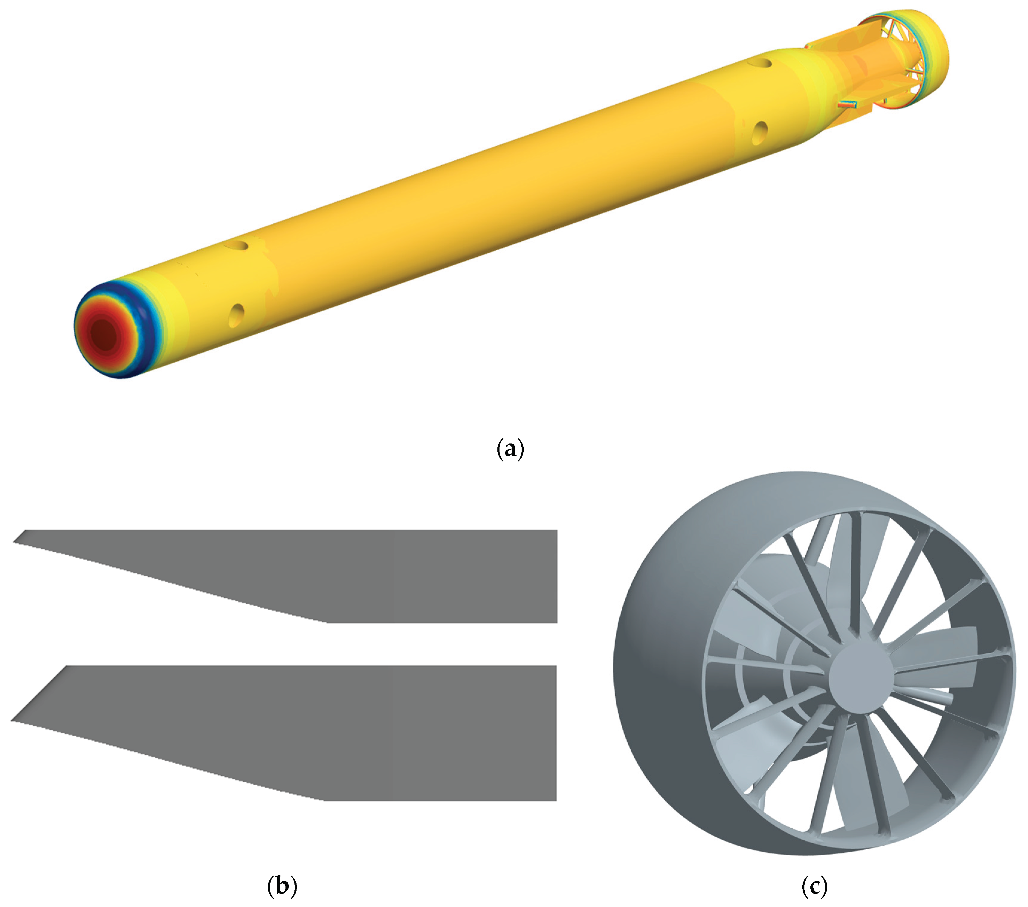
Figure 2.
Surface grids on AUV and y=0 plane: (a) near AUV nose; (b) near stern; (c) propeller blades; (d) propulsion system including a duct and struts.
Figure 2.
Surface grids on AUV and y=0 plane: (a) near AUV nose; (b) near stern; (c) propeller blades; (d) propulsion system including a duct and struts.
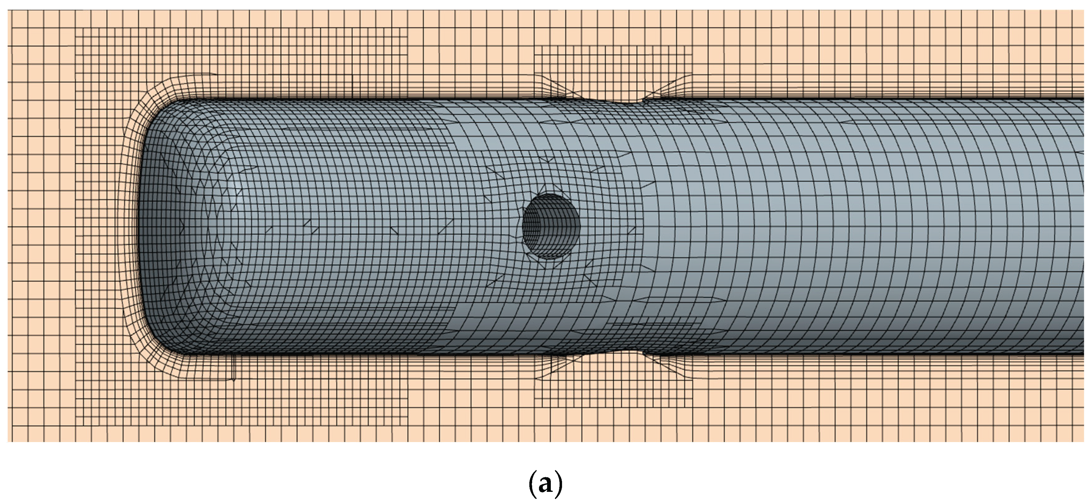
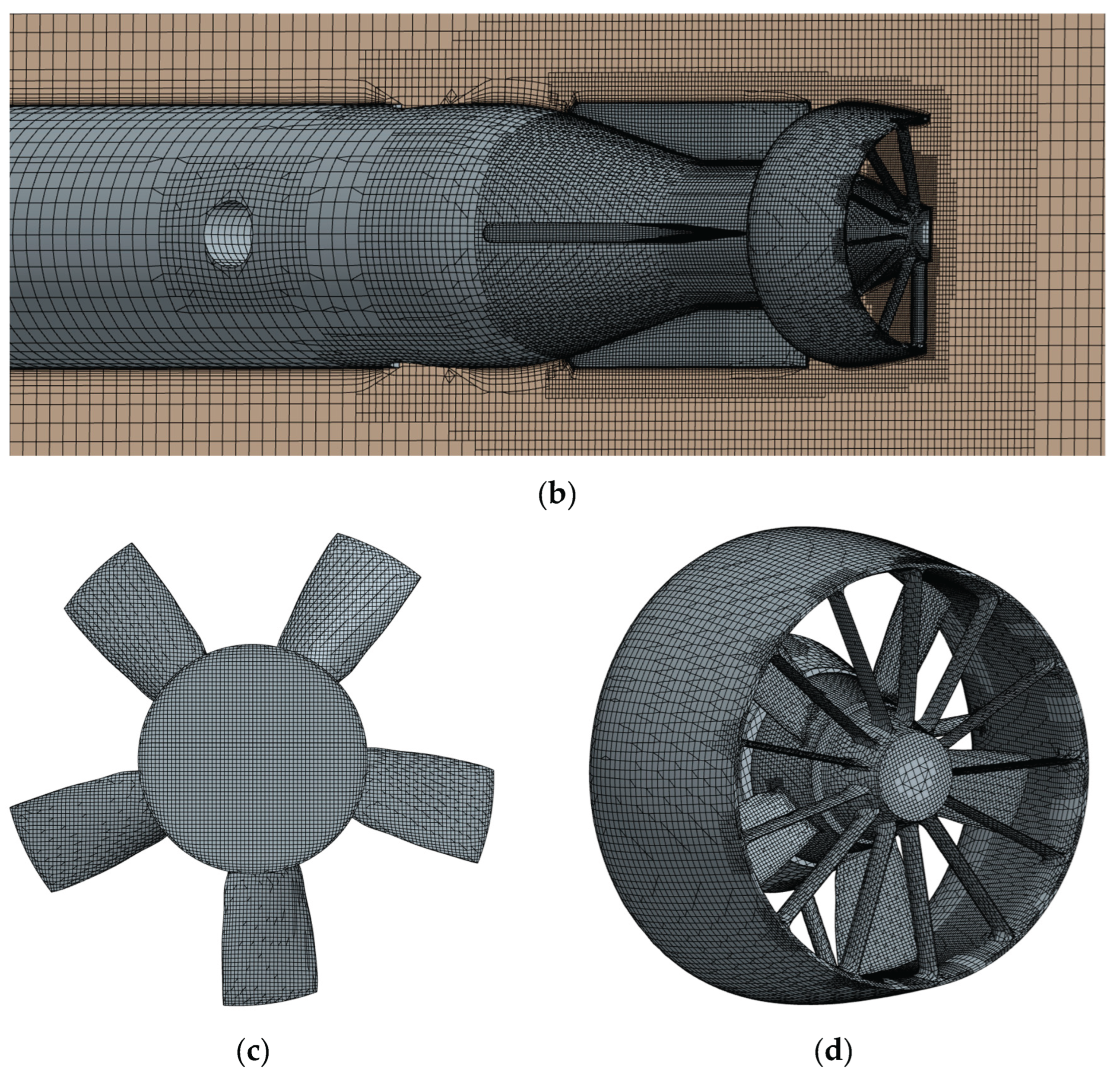
Figure 3.
Overset configuration demonstration: Overset regions for 4 rudders are shown
Figure 4.
Computation domain size.
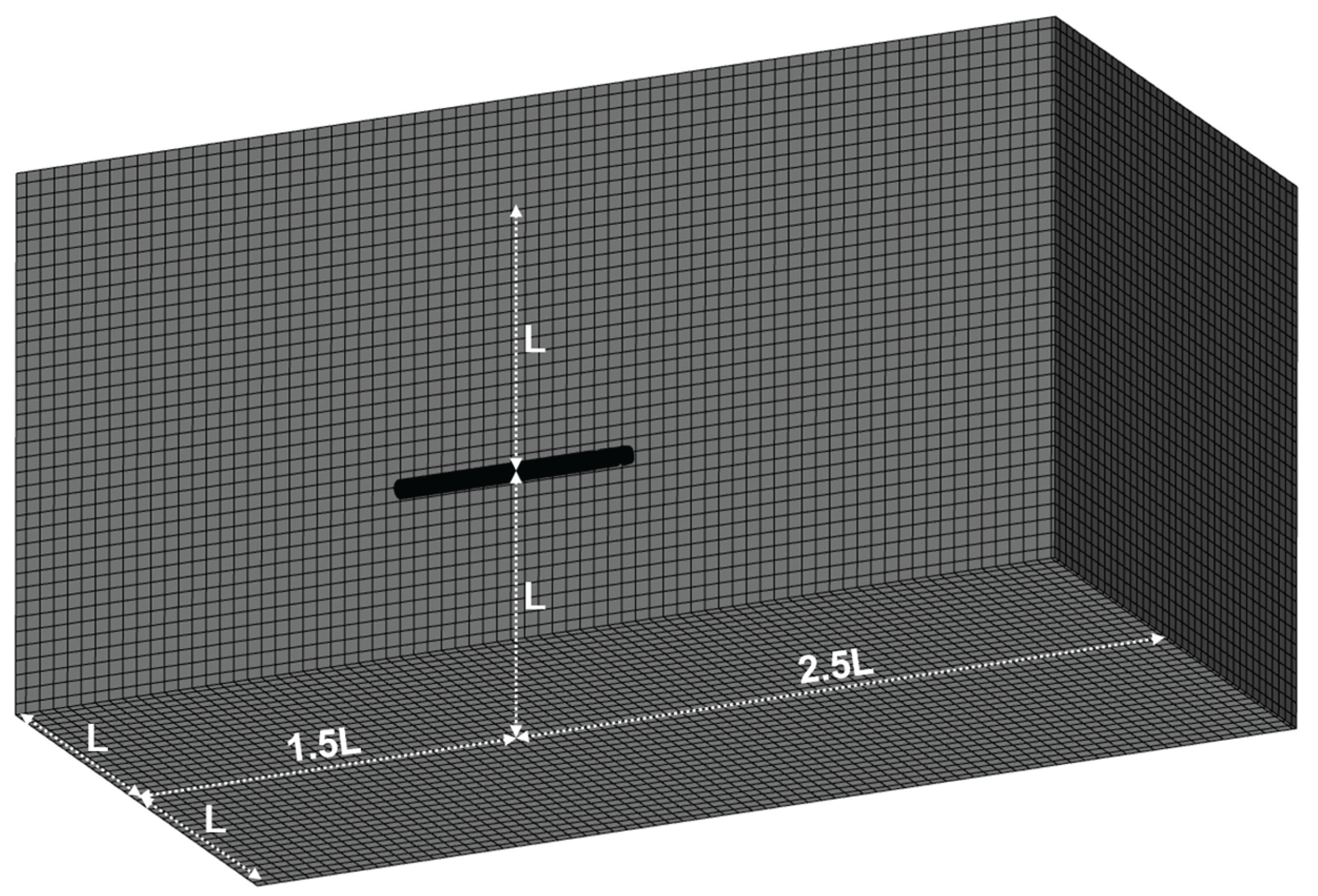
Figure 5.
Sectional area for obtaining averaged axial-speed at the duct inlet.
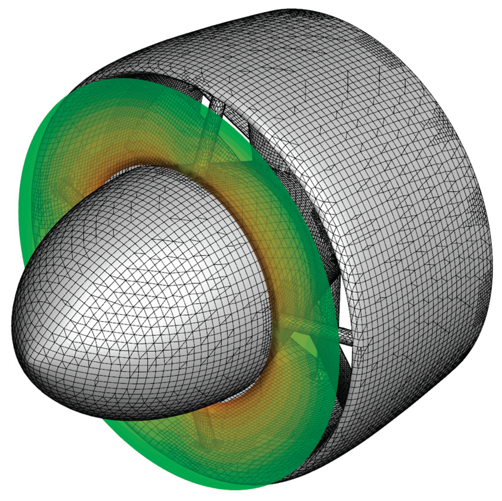
Figure 6.
Surrogate algorithm flowchart.
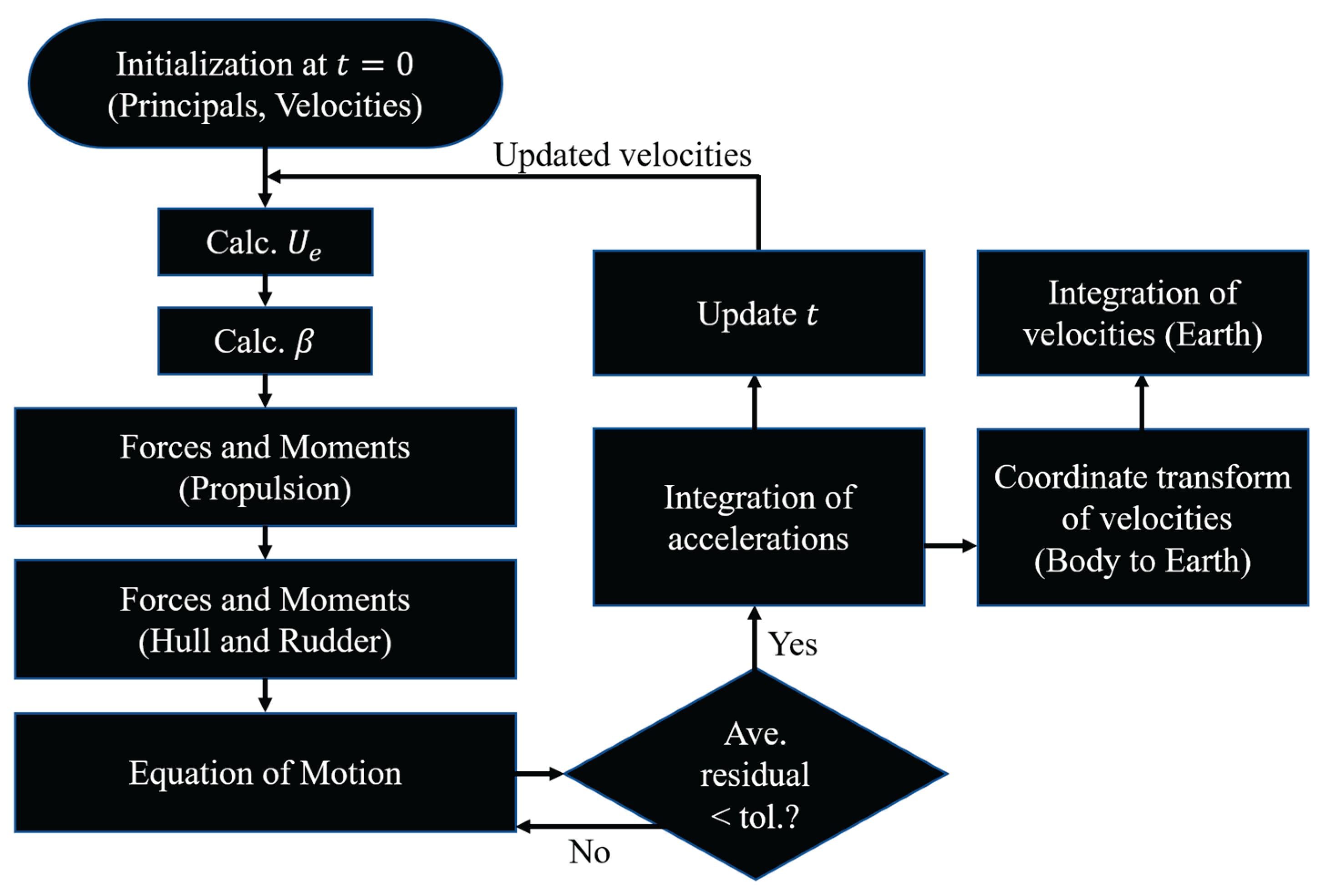
Figure 7.
Propeller wake in POW simulation with a discretized propeller model (Q=10).
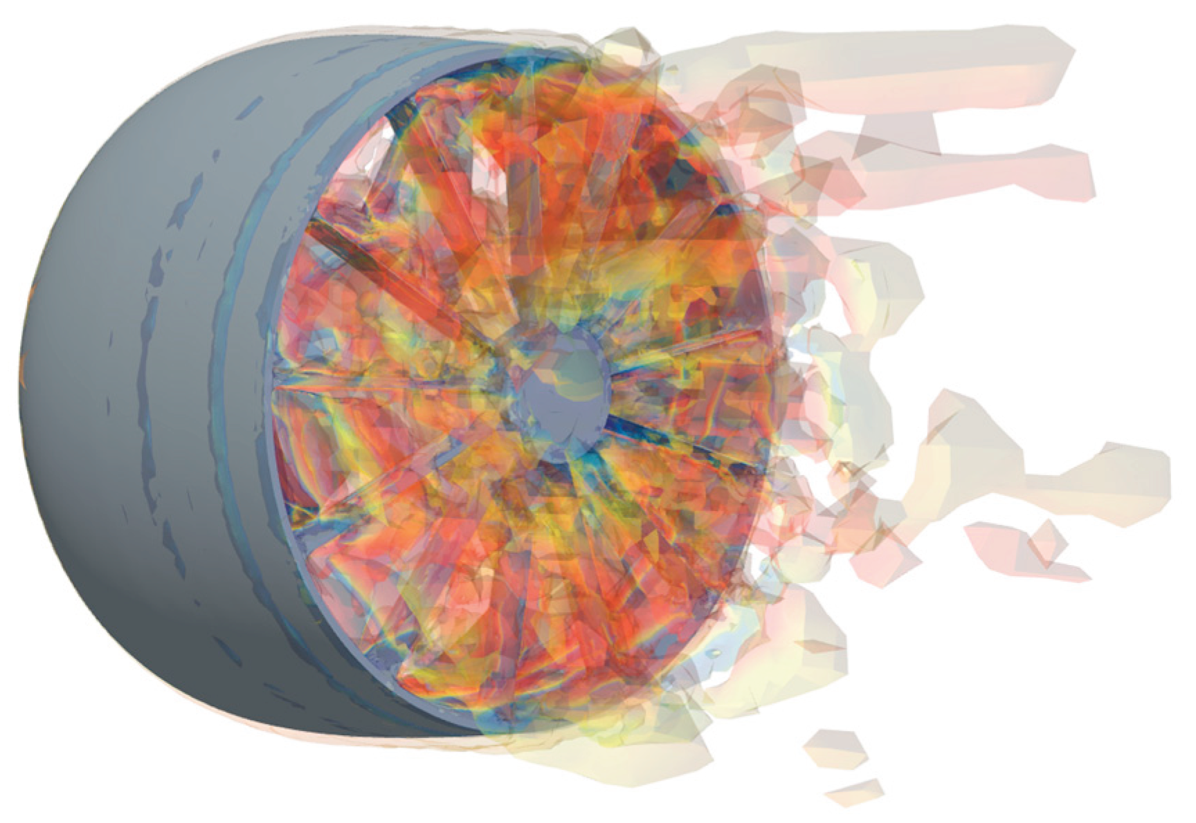
Figure 8.
POW characteristic curves obtained via grid triplets of discretized propeller model: (a) thrust coefficient; (b) torque coefficient; (c) propeller open water efficiency; (d) duct resistance.
Figure 8.
POW characteristic curves obtained via grid triplets of discretized propeller model: (a) thrust coefficient; (b) torque coefficient; (c) propeller open water efficiency; (d) duct resistance.
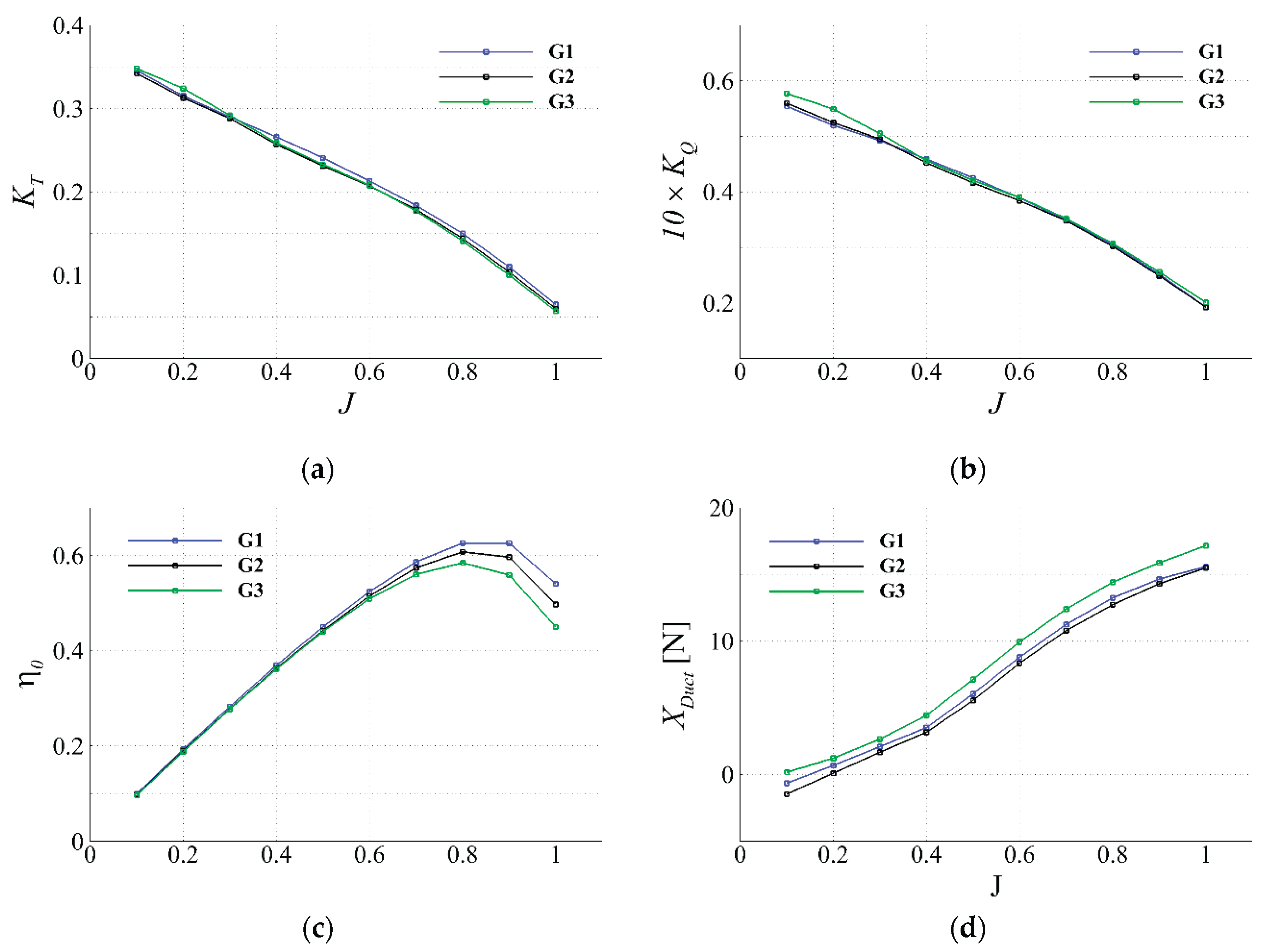
Figure 9.
Correlation between and achieved from POW simulations using G2 DP model.
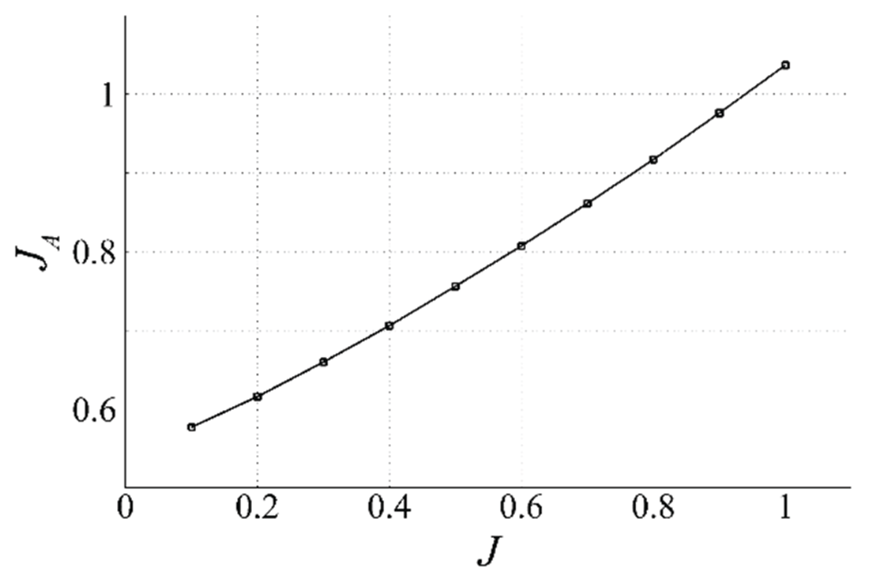
Figure 10.
Grid triplet’s axial inflow speed distribution at duct inlet (left: G1, middle: G2, right: G3): (a) ; (b) ; (c) .
Figure 10.
Grid triplet’s axial inflow speed distribution at duct inlet (left: G1, middle: G2, right: G3): (a) ; (b) ; (c) .
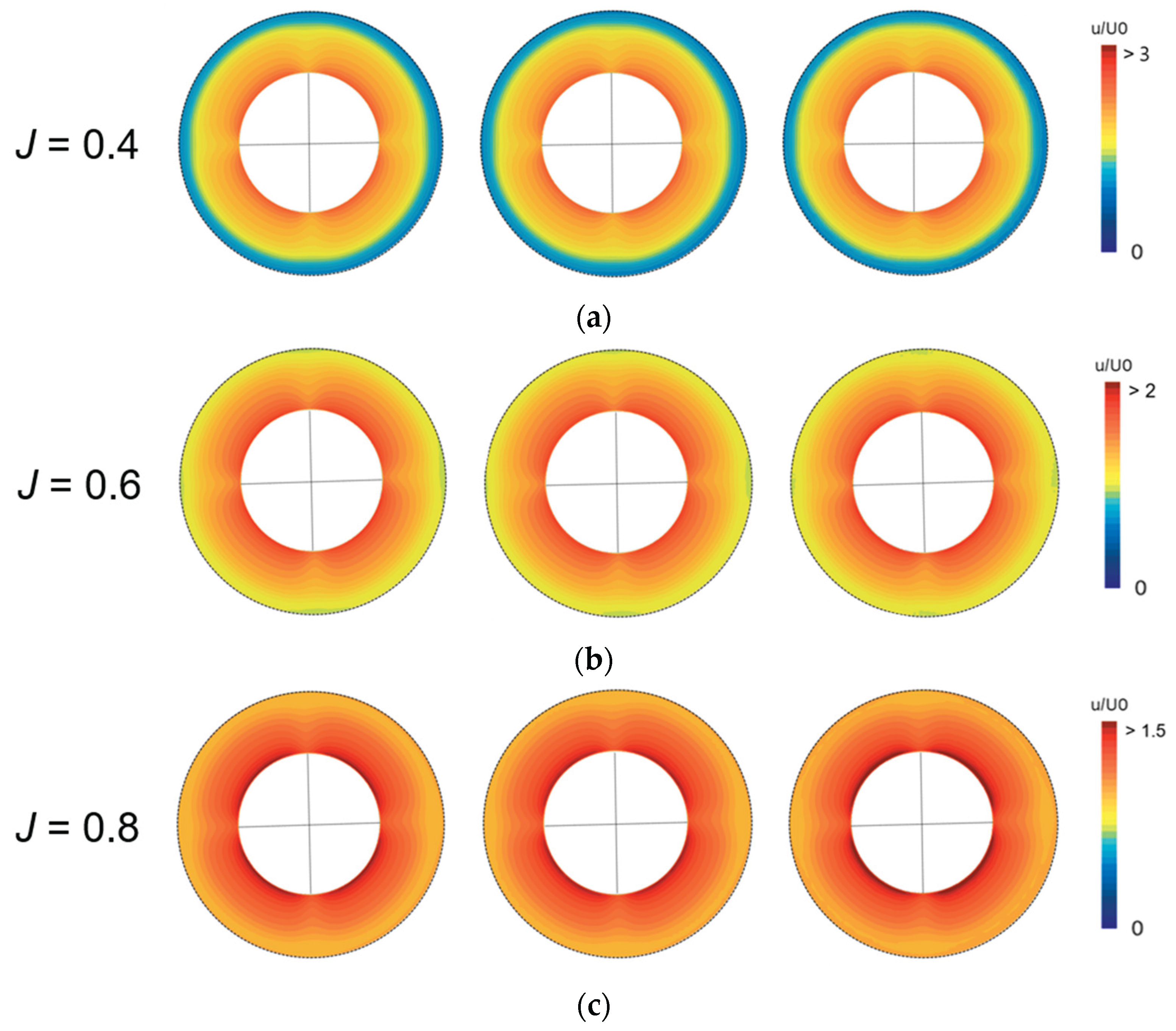
Figure 11.
Validation of CFD BF model against DP model: (a) thrust coefficient; (b) torque coefficient; (c) propeller open-water efficiency; (d) advance coefficient at duct inlet.
Figure 11.
Validation of CFD BF model against DP model: (a) thrust coefficient; (b) torque coefficient; (c) propeller open-water efficiency; (d) advance coefficient at duct inlet.
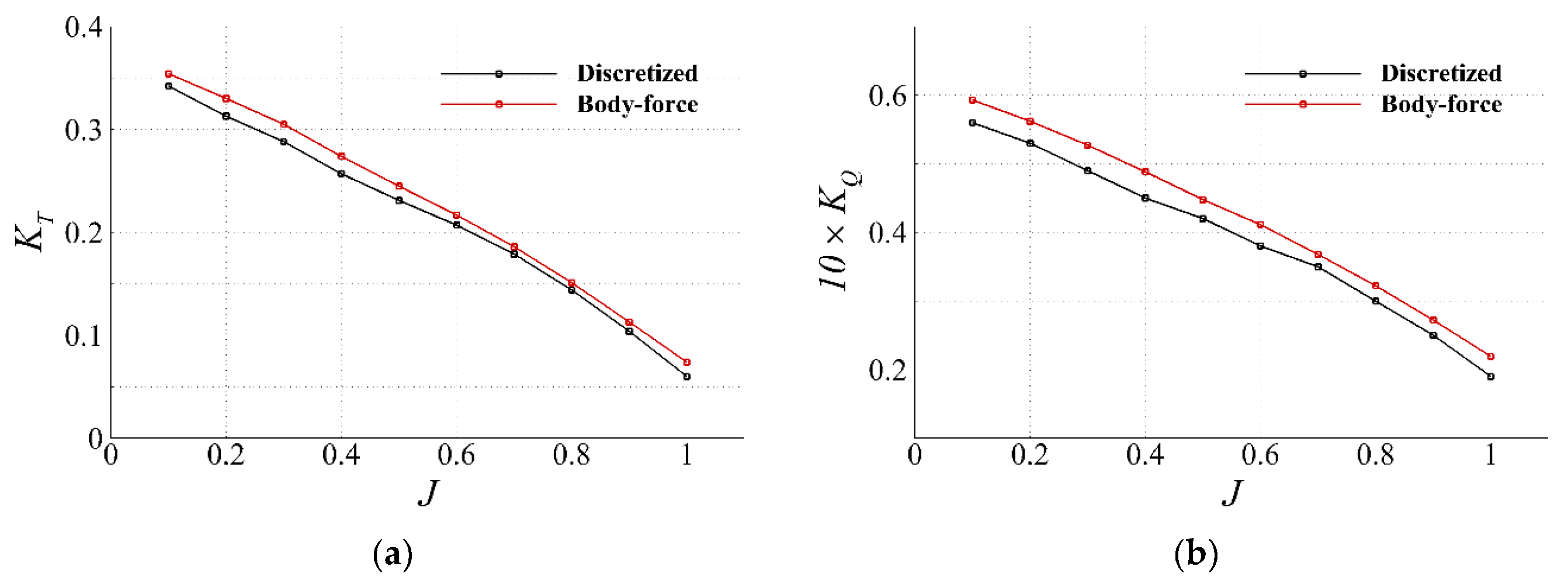
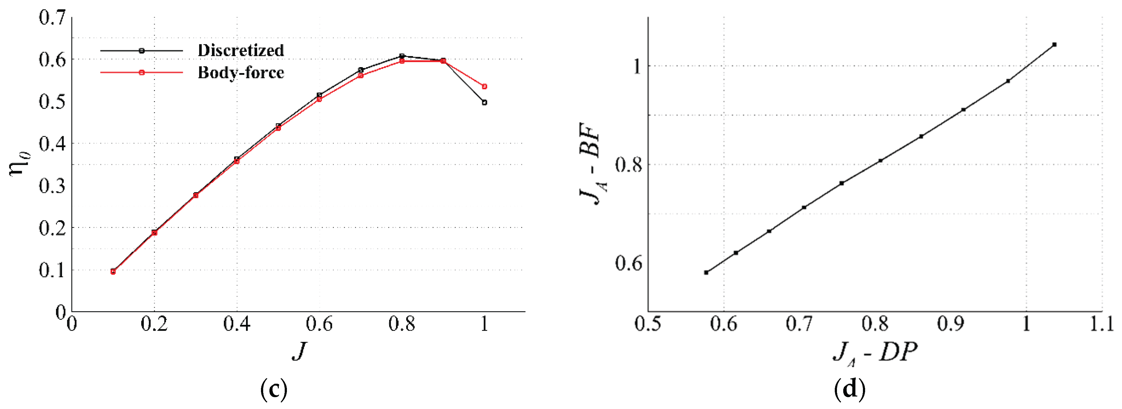
Figure 12.
Axial inflow speed distribution near the propulsion system: (a) DP model; (b) BF model.
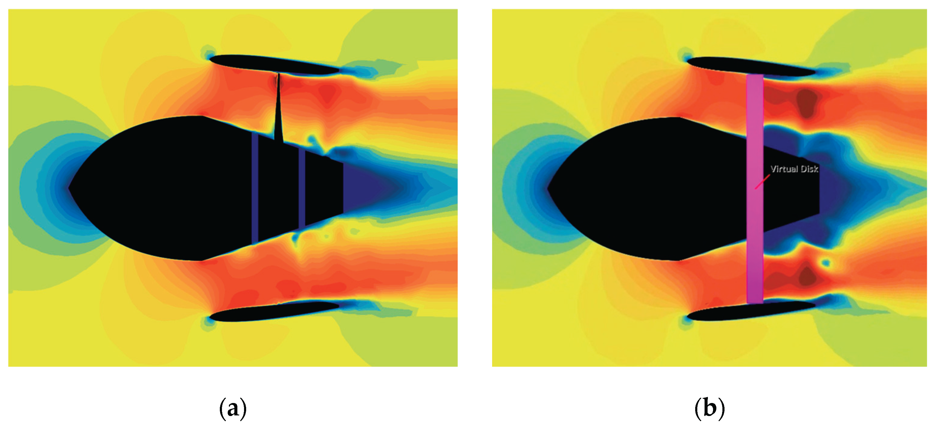
Figure 13.
Pressure distribution at the steady state of resistance simulation.
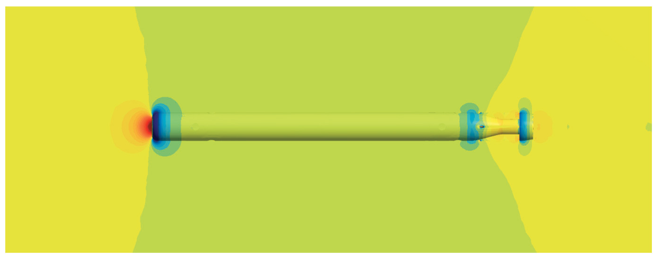
Figure 14.
Resistance test results: (a) resistance curve against Froude number; (b) frictional resistance curve against Froude number.
Figure 14.
Resistance test results: (a) resistance curve against Froude number; (b) frictional resistance curve against Froude number.
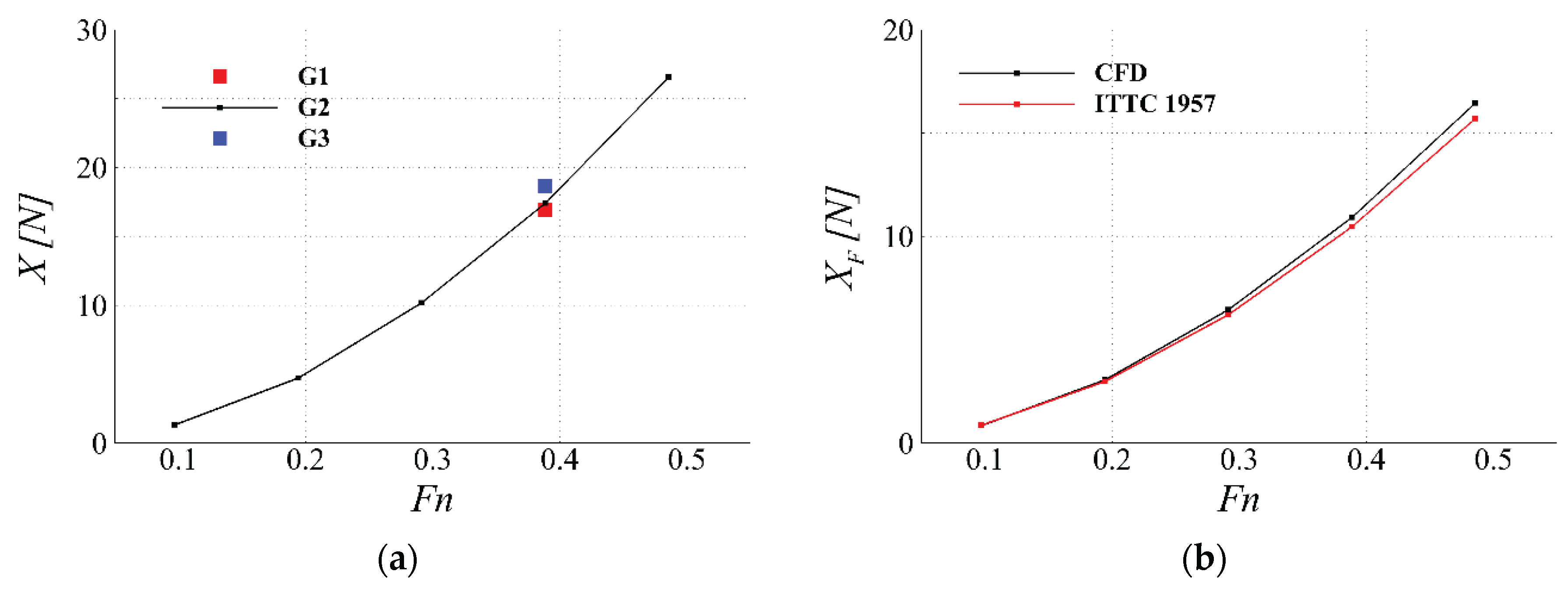
Figure 15.
Grid triplet’s axial inflow speed at the duct inlet during resistance simulation: (a) G1; (b) G2; (c) G3.
Figure 15.
Grid triplet’s axial inflow speed at the duct inlet during resistance simulation: (a) G1; (b) G2; (c) G3.
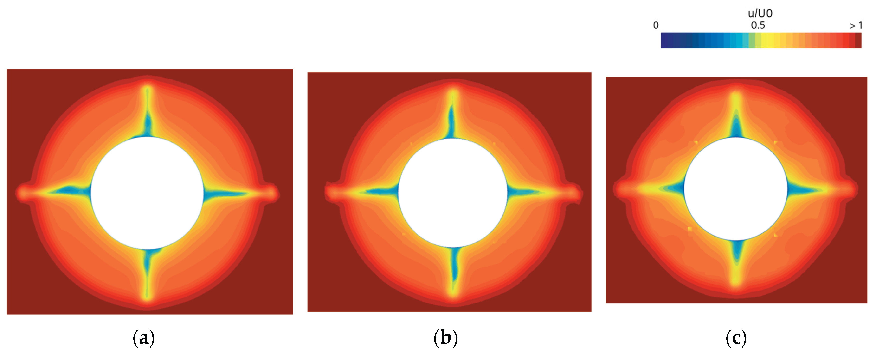
Figure 16.
Pressure distribution and propeller wake (Q = 10) during self-propulsion simulation.
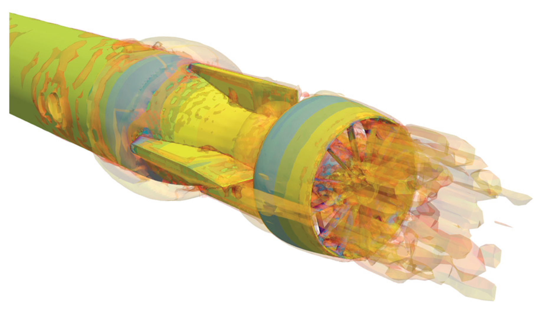
Figure 17.
Self-propulsion simulation results at target Froude number: (a) propeller rotational speed tested for finding self-propulsion point; (b) time-history of ship speed represented as instantaneous Froude number during self-propulsion simulation using zero initial ship speed and propeller rotational speed found at self-propulsion point.
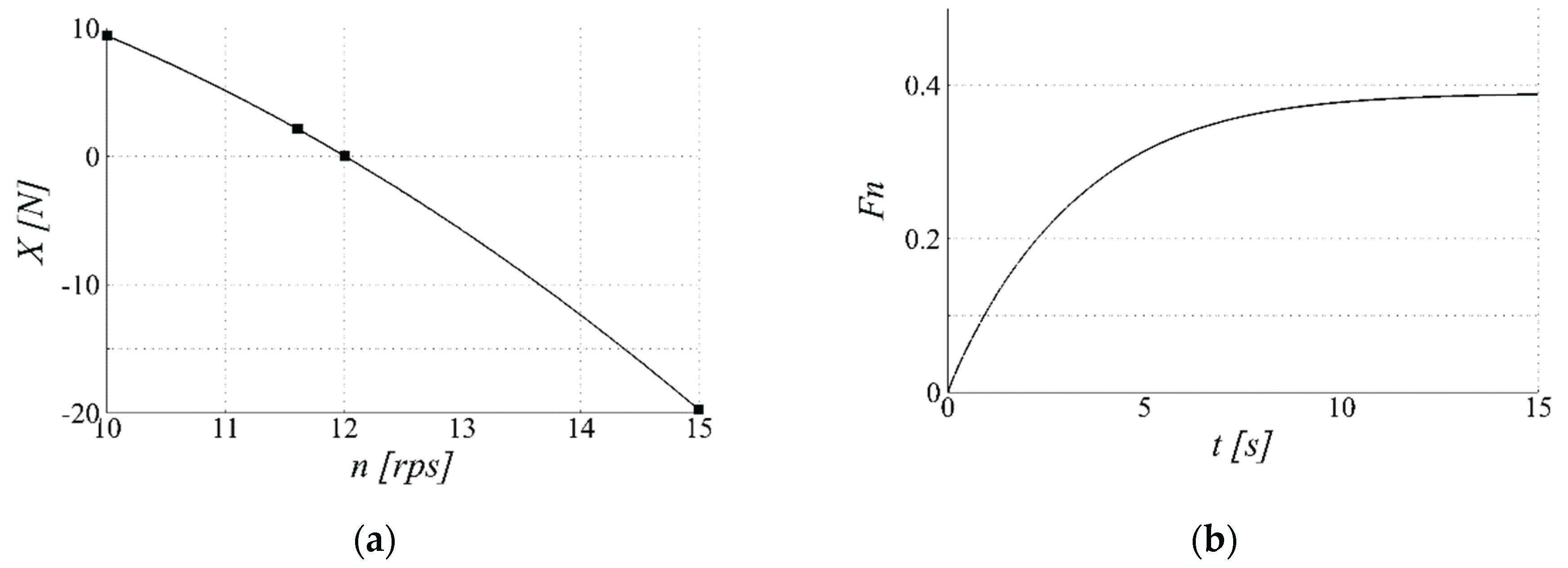
Figure 18.
Pressure distributions: (a) static-drift (; (b) control-fin simulation (.
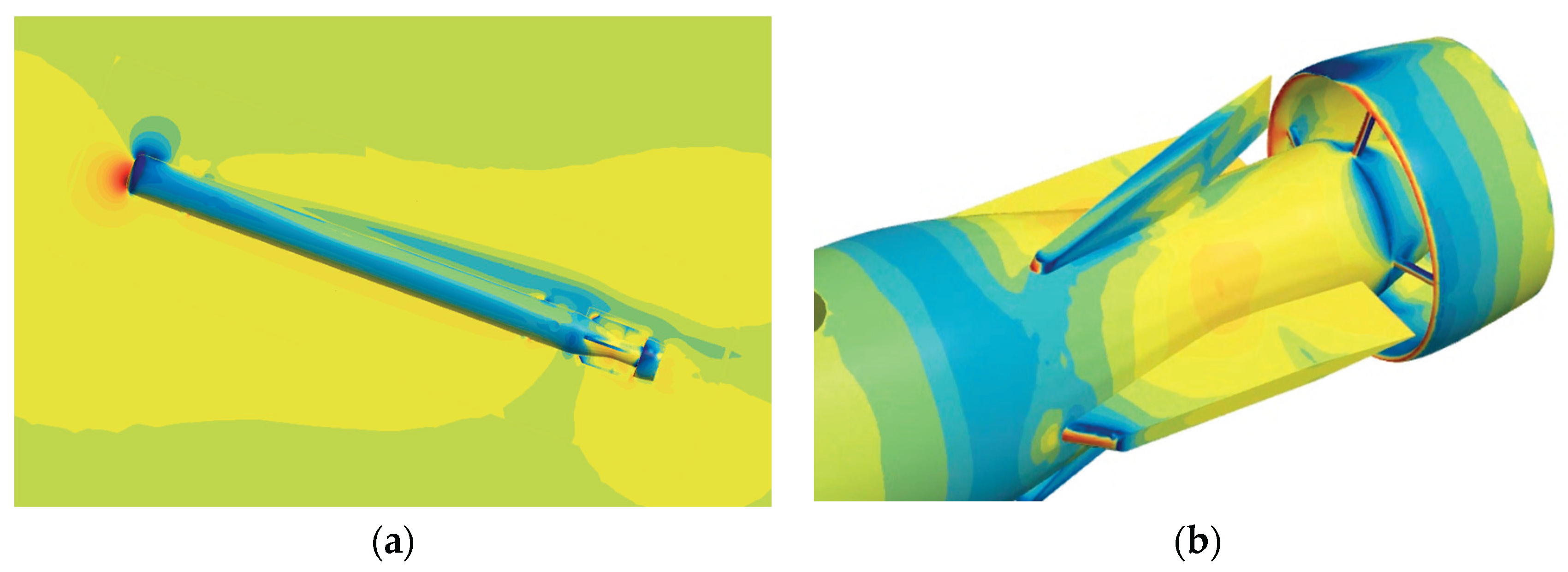
Figure 19.
Measured forces and moment and regression curve for Surrogate in static-drift simulations: (a) surge force; (b) sway force; (c) yaw moment, and control-fin simulation: (d) surge force; (e) sway force; (f) yaw moment.
Figure 19.
Measured forces and moment and regression curve for Surrogate in static-drift simulations: (a) surge force; (b) sway force; (c) yaw moment, and control-fin simulation: (d) surge force; (e) sway force; (f) yaw moment.
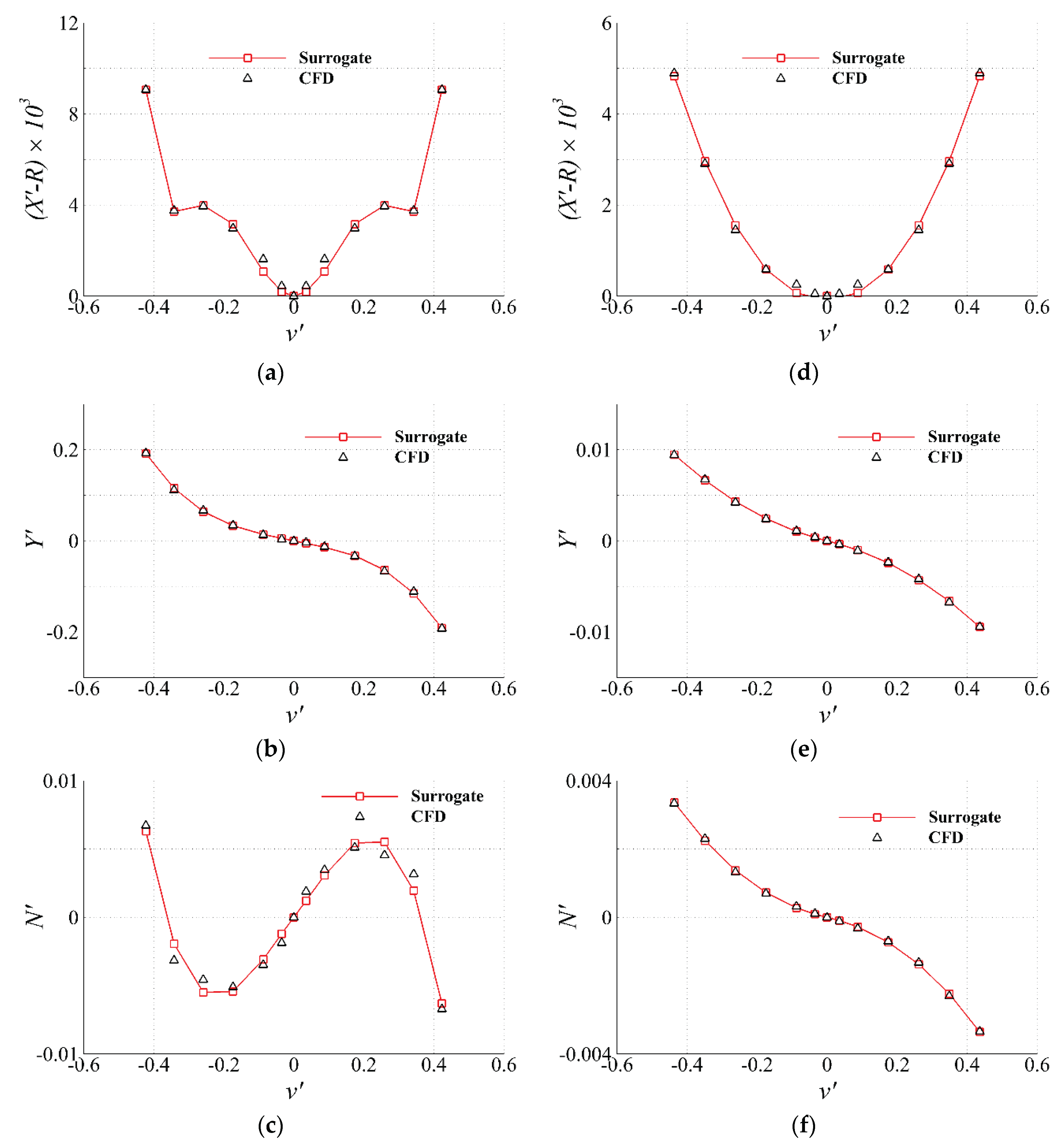
Figure 20.
The measured time-histories: (a) sway displacement, velocity and acceleration from both pure-sway and pure-yaw; (b) sway force from pure-sway; (c) yaw moment from pure-sway; (d) yaw displacement, velocity and acceleration from pure-yaw; (e) sway force from pure-yaw; (f) yaw moment from pure-yaw.
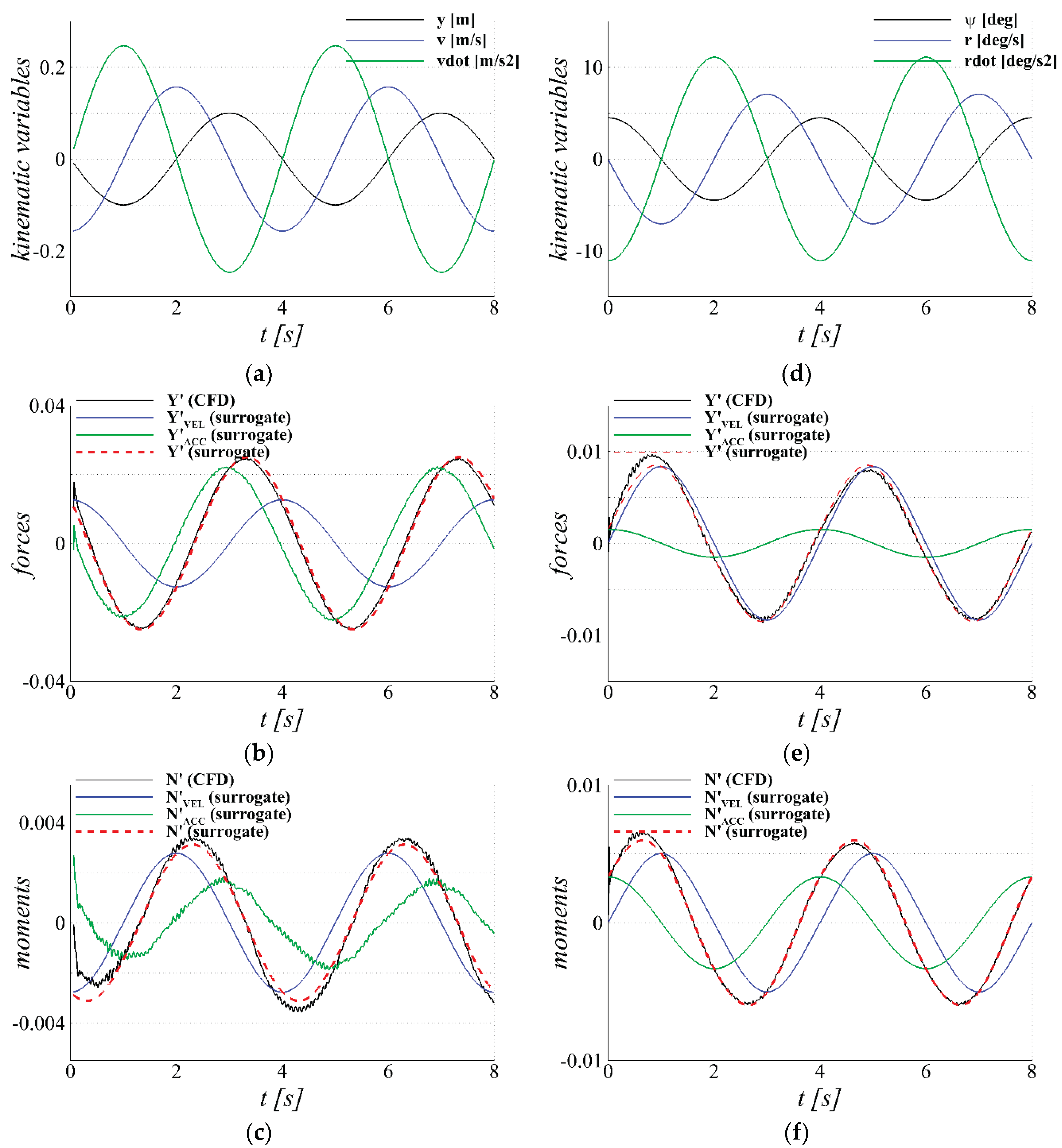
Figure 21.
The measured time-histories during forced-oscillation simulation: (a) sway displacement, velocity and acceleration; (b) sway force.
Figure 21.
The measured time-histories during forced-oscillation simulation: (a) sway displacement, velocity and acceleration; (b) sway force.
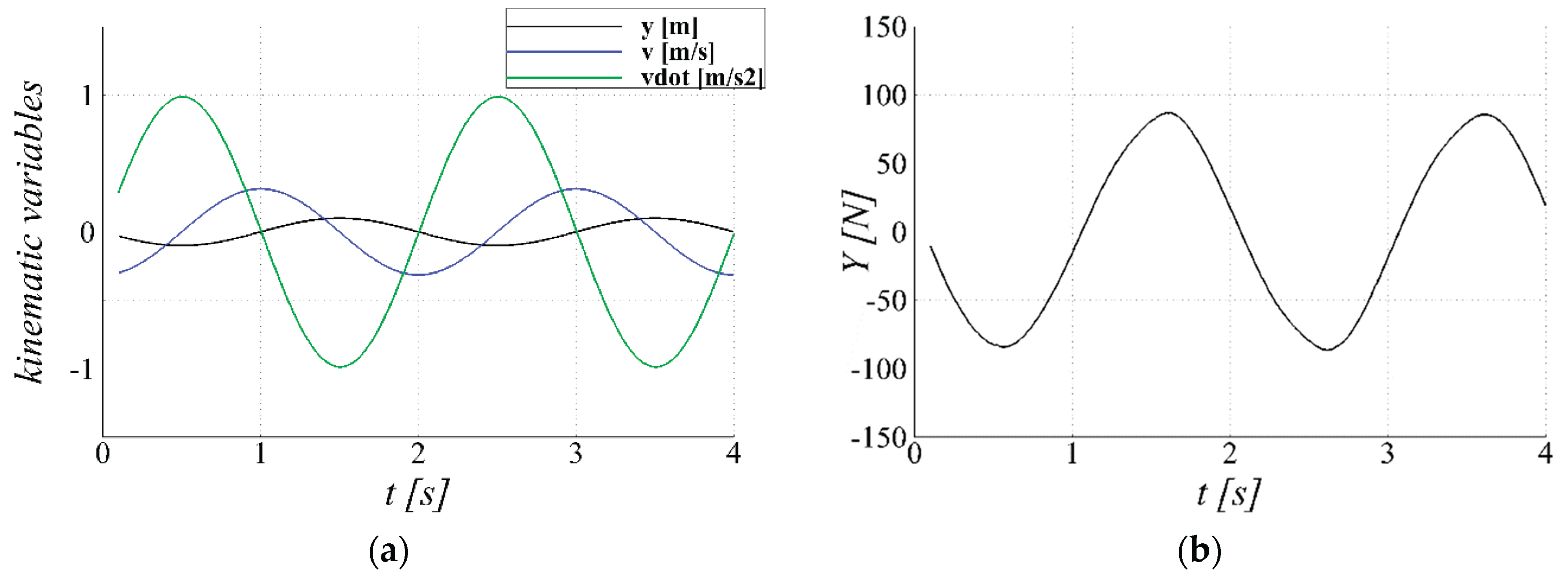
Figure 22.
Time-histories of kinematic variables and advance coefficient at the duct inlet during free-running zigzag simulations: (a) trajectory; (b) ship axial speed; (c) ship lateral speed; (d) advance coefficient at the duct inlet; (e) yaw speed; (f) drift-angle; (g) yaw and rudder angles.
Figure 22.
Time-histories of kinematic variables and advance coefficient at the duct inlet during free-running zigzag simulations: (a) trajectory; (b) ship axial speed; (c) ship lateral speed; (d) advance coefficient at the duct inlet; (e) yaw speed; (f) drift-angle; (g) yaw and rudder angles.
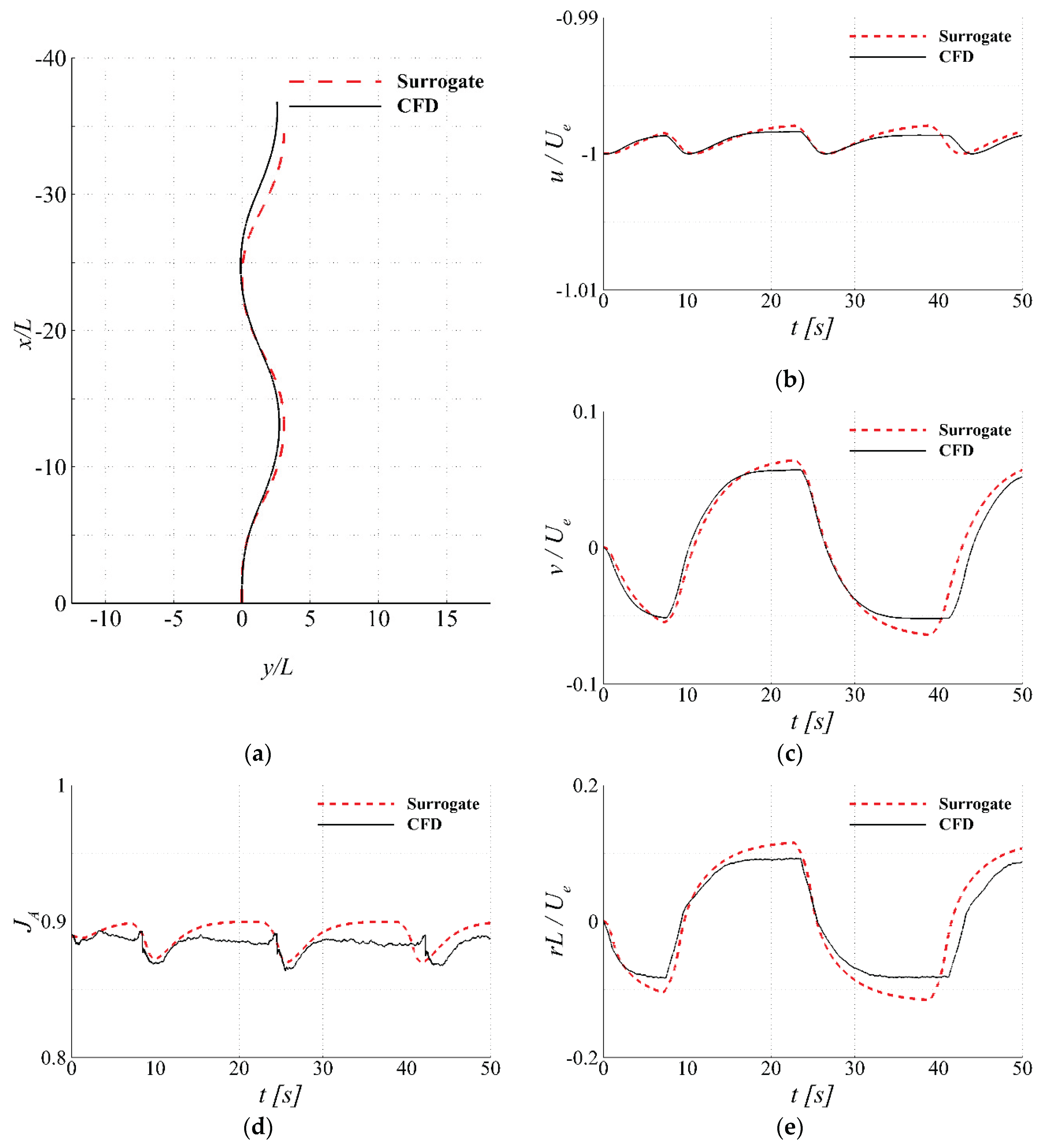
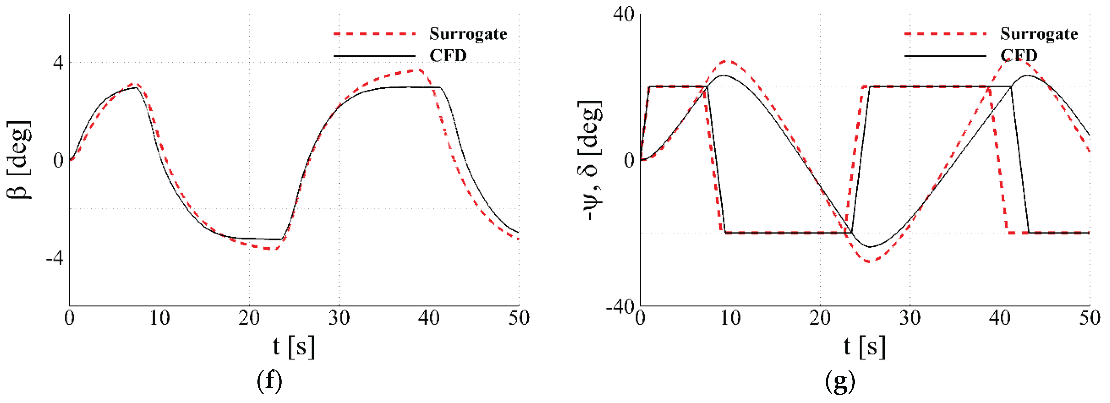
Figure 23.
Time-histories of forces and moment during free-running zigzag simulations: (a) total surge force; (b) total sway force; (c) total yaw moment; (d) propeller thrust.
Figure 23.
Time-histories of forces and moment during free-running zigzag simulations: (a) total surge force; (b) total sway force; (c) total yaw moment; (d) propeller thrust.
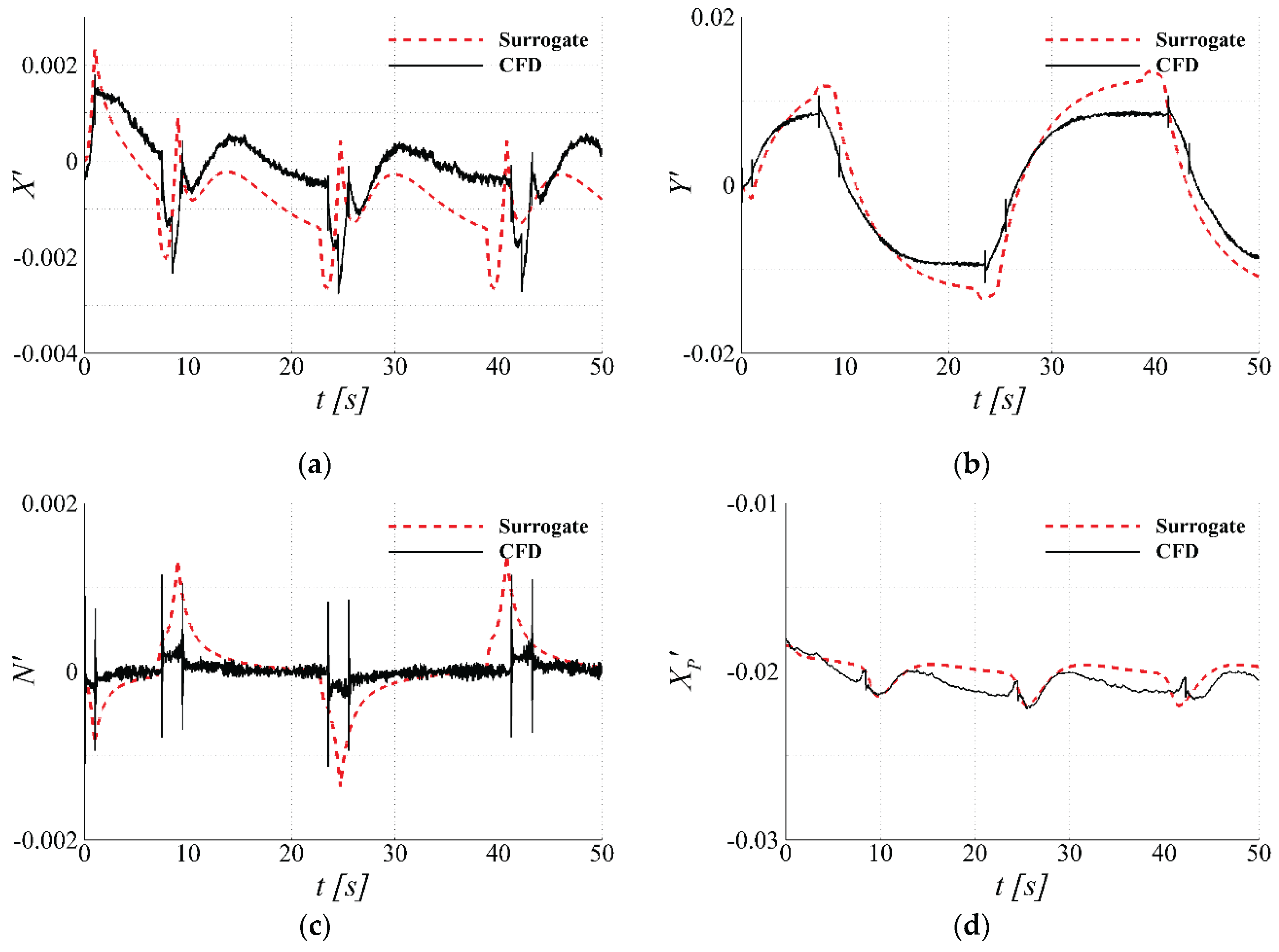
Table 1.
Main principals (Fully-attached AUV)
| Description | Symbol | Factor1 | Value2 |
|---|---|---|---|
| Breadth | 0.074 | ||
| Mass | 3.830e-3 | ||
| Center of gravity3 (x-dir.) | 0.463 | ||
| Radius of gyration (z-dir.) | 0.166 | ||
| Moment of inertia (z-dir.) | 1.059e-4 | ||
| Location of rudder axis3 (x-dir.) | 0.904 | ||
| Location of propeller center3 (x-dir.) | 0.982 | ||
| Propeller diameter | 0.063 |
1 Factor for non-dimensionalization. is used; 2 Dimensionless value; 3 Distance from the nose of AUV
Table 2.
Number of grid points of grid triplet for POW simulation.
| Region | # of cells [M] | ||
|---|---|---|---|
| G1 | G2 | G3 | |
| Blade | 0.79 | 0.41 | 0.24 |
| Duct | 1.67 | 0.83 | 0.46 |
| Background | 0.07 | 0.04 | 0.03 |
| Total | 2.53 | 1.28 | 0.73 |
Table 3.
Number of grid points of grid triplet for simulations including hull and rudders.
| Region | # of cells [M] | ||
|---|---|---|---|
| G1 | G2 | G3 | |
| Hull* | 3.02 | 1.47 | 0.78 |
| Rudders | 0.86 | 0.35 | 0.14 |
| Background | 0.17 | 0.07 | 0.03 |
| Total | 4.05 | 1.89 | 0.95 |
* includes Duct
Table 4.
Boundary conditions.
| BC | * | |||
|---|---|---|---|---|
| Inlet | Extrapolated | |||
| Exit | Extrapolated | Extrapolated | Zero-gradient | Zero-gradient |
| Wall | Grid velocity | Zero-gradient | Zero-gradient | Zero-gradient |
*
Table 5.
Simulation test-matrix.
| Simulation | Condition | Grid system |
|---|---|---|
| Hydrostatic | Static | G2 |
| POW (discretized) | = 0.1 - 1.0 | G1, G2, G3 |
| POW (body-force) | = 0.1 - 1.0 | G2 |
| Resistance | Fn = 0.097, 0.19, 0.29, 0.39, 0.48 | G1, G2, G3 |
| Self-propulsion1 | Fn = 0.39 | G2 |
| Static-drift | = 2, 5, 10, 15, 20, 25 [deg] | G2 |
| Control-fin | = 2, 5, 10, 15, 20, 25 [deg] | G2 |
| Pure-sway | y = (0.1)sin(0.5πt), Fn = 0.39 | G2 |
| Pure-yaw2 | ψ=(0.1/)cos(0.5πt) | G2 |
| Forced-oscillation | y = (0.1)sin(πt), Fn = 0 | G2 |
| Zigzag1 | = +20/20 | G2 |
1 Simulation performed with propulsion; 2 Conditions for y and Fn is identical to Pure-sway’s
Table 6.
results from POW simulations using grid triplets with the DP model.
| 0.1 | 0.346 | 0.342 | 0.348 | -1.1 | 1.6 | -0.72 |
| 0.2 | 0.315 | 0.313 | 0.324 | -0.7 | 3.5 | -0.2 |
| 0.3 | 0.29 | 0.288 | 0.292 | -0.8 | 1.5 | -0.51 |
| 0.4 | 0.266 | 0.257 | 0.259 | -3.3 | 0.6 | -5.04 |
| 0.5 | 0.241 | 0.231 | 0.233 | -3.8 | 0.5 | -7.11 |
| 0.6 | 0.213 | 0.207 | 0.208 | -2.8 | 0.4 | -7.91 |
| 0.7 | 0.184 | 0.179 | 0.177 | -2.7 | -1.2 | 2.25 |
| 0.8 | 0.15 | 0.144 | 0.141 | -4.3 | -1.9 | 2.24 |
| 0.9 | 0.11 | 0.104 | 0.1 | -5.8 | -3.2 | 1.82 |
| 1 | 0.065 | 0.06 | 0.057 | -8.3 | -4.8 | 1.73 |
| Abs. Ave.* | 3.4 | 1.9 |
* absolute average
Table 7.
results from POW simulations using grid triplets with the DP model .
| 0.1 | 0.0554 | 0.056 | 0.0577 | 1 | 3.1 | 0.33 |
| 0.2 | 0.052 | 0.0525 | 0.0549 | 1 | 4.6 | 0.22 |
| 0.3 | 0.0492 | 0.0495 | 0.0505 | 0.6 | 2.1 | 0.29 |
| 0.4 | 0.0459 | 0.0452 | 0.0456 | -1.6 | 1 | -1.63 |
| 0.5 | 0.0425 | 0.0416 | 0.0421 | -2.1 | 1.1 | -1.81 |
| 0.6 | 0.0389 | 0.0384 | 0.039 | -1.2 | 1.5 | -0.79 |
| 0.7 | 0.035 | 0.0348 | 0.0352 | -0.8 | 1.2 | -0.65 |
| 0.8 | 0.0305 | 0.0302 | 0.0307 | -1.2 | 1.8 | -0.66 |
| 0.9 | 0.0252 | 0.0249 | 0.0256 | -1 | 2.9 | -0.35 |
| 1 | 0.0193 | 0.0192 | 0.0201 | -0.5 | 4.7 | -0.1 |
| Abs. Ave. | 1.1 | 2.4 |
Table 8.
results from POW simulations using grid triplets with the DP model .
| 0.1 | 0.099 | 0.097 | 0.096 | -2.1 | -1.4 | 1.54 |
| 0.2 | 0.193 | 0.19 | 0.188 | -1.7 | -1 | 1.77 |
| 0.3 | 0.282 | 0.278 | 0.277 | -1.4 | -0.5 | 2.95 |
| 0.4 | 0.369 | 0.363 | 0.361 | -1.7 | -0.3 | 5.1 |
| 0.5 | 0.45 | 0.442 | 0.44 | -1.8 | -0.6 | 3.03 |
| 0.6 | 0.524 | 0.515 | 0.509 | -1.6 | -1.2 | 1.42 |
| 0.7 | 0.586 | 0.574 | 0.56 | -2 | -2.4 | 0.84 |
| 0.8 | 0.626 | 0.607 | 0.584 | -3.1 | -3.6 | 0.86 |
| 0.9 | 0.626 | 0.596 | 0.559 | -4.8 | -5.8 | 0.83 |
| 1 | 0.54 | 0.497 | 0.45 | -7.9 | -8.8 | 0.9 |
| Abs. Ave. | 2.8 | 2.6 |
Table 9.
, , and values measured from POW simulations using G2 DP model. .
| 0.1 | 0.255 | 1.472 | 0.577 |
| 0.2 | 0.510 | 1.571 | 0.616 |
| 0.3 | 0.765 | 1.684 | 0.660 |
| 0.4 | 1.020 | 1.802 | 0.706 |
| 0.5 | 1.275 | 1.927 | 0.756 |
| 0.6 | 1.530 | 2.059 | 0.807 |
| 0.7 | 1.785 | 2.195 | 0.861 |
| 0.8 | 2.040 | 2.339 | 0.917 |
| 0.9 | 2.295 | 2.488 | 0.976 |
| 1.0 | 2.550 | 2.644 | 1.037 |
Table 10.
Coefficients of POW characteristics regression curve built upon .
| Coefficient | Value | Coefficient | Value |
|---|---|---|---|
| 0.3582 | 0.0582 | ||
| -0.1993 | -0.0256 | ||
| -0.0937 | -0.0128 |
Table 11.
Coefficients of POW characteristics regression curve built upon .
| Coefficient | Value | Coefficient | Value |
|---|---|---|---|
| 0.6187 | 0.0919 | ||
| -0.4329 | -0.0551 | ||
| -0.0981 | -0.0140 |
Table 12.
Coefficients of resistance regression curve (Figure 14(a)).
Table 12.
Coefficients of resistance regression curve (Figure 14(a)).
| Coefficient | Value |
|---|---|
| -0.2792 | |
| 6.5738 | |
| 100.212 |
Table 16.
Coefficients of regression curves achieved from pure-yaw simulations.
| Coefficient | Value | Coefficient | Value |
|---|---|---|---|
| -0.04458 | -0.02690 | ||
| -0.03431 | -0.01989 | ||
| -0.00432 | -0.00944 |
Disclaimer/Publisher’s Note: The statements, opinions and data contained in all publications are solely those of the individual author(s) and contributor(s) and not of MDPI and/or the editor(s). MDPI and/or the editor(s) disclaim responsibility for any injury to people or property resulting from any ideas, methods, instructions or products referred to in the content. |
© 2025 by the authors. Licensee MDPI, Basel, Switzerland. This article is an open access article distributed under the terms and conditions of the Creative Commons Attribution (CC BY) license (http://creativecommons.org/licenses/by/4.0/).
Copyright: This open access article is published under a Creative Commons CC BY 4.0 license, which permit the free download, distribution, and reuse, provided that the author and preprint are cited in any reuse.


